Pumping Station Design in Water Distribution Networks Considering the Optimal Flow Distribution between Sources and Capital and Operating Costs

Abstract

The investment and operating costs of pumping stations in drinking water distribution networks are some of the highest public costs in urban sectors. Generally, these systems are designed based on extreme scenarios. However, in periods of normal operation, extra energy is produced, thereby generating excess costs. To avoid this problem, this work presents a new methodology for the design of pumping stations. The proposed technique is based on the use of a setpoint curve to optimize the operating and investment costs of a station simultaneously. According to this purpose, a novel mathematical optimization model is developed. The solution output by the model includes the selection of the pumps, the dimensions of pipelines, and the optimal flow distribution among all water sources for a given network. To demonstrate the advantages of using this technique, a case study network is presented. A pseudo-genetic algorithm (PGA) is implemented to resolve the optimization model. Finally, the obtained results show that it is possible to determine the full design and operating conditions required to achieve the lowest cost in a multiple pump station network.

1. Introduction

Optimization problems regarding the design and operation of water distribution networks (WDNs) are very complex and important problems that affect the quality of life of all people worldwide [1]. The demand for water increases rapidly with the growth of the world’s population. Furthermore, climate change has increased water scarcity [2]. Electric power is one of the dominant costs incurred by water utilities, so reducing energy consumption and conserving the available natural resources (such as water) are some of society’s challenges [3]. The design of a cost-effective WDN is not a simple task, and the operational performance of the designed network affects any city budget [4,5]. In this regard, pumping stations (PSs) are expensive infrastructures.

Pump operating costs are a key aspect when a network is fed directly from groundwater or does not have a high enough elevation for tanks to be installed [5]. In these cases, the selection of pumps that best adapt to the system head curve is an important step, as doing so reduces excess head pressure [6]. Consequently, the efficient design and operation of PSs could significantly reduce network total costs.

PS design involves the selection of pumps, accessories, and control systems. Traditionally, the selection process is conducted by a catalogue that contains the specifications of available pumps. The pumps that provide the required maximum piezometric head are identified, and the selection is based, among other criteria, on energy efficiency. Finally, the number of pumps that make up the station is calculated [7]. Then, PS operation is determined by the on/off status of every pump at each time step and, in the case of variable-speed pumps (VSPs), by modifying the rotational speed based on the readings obtained from the metering devices.

This control system is responsible for adjusting the amount of water pumped according to public demand at every moment [8]. Different approaches for improving PS performance in WDNs have been explored [1,9,10]. One of the important problems covered in the literature is pump scheduling optimization. This problem has been widely studied [3,9]. Starting from a completed PS design, pump scheduling can be specified by on/off pump switches during predefined equal time intervals. Traditionally, the objective of such a problem is the minimization of energy consumption costs based on the operation and/or maintenance costs of pumps [3]. These approaches do not allow for any structural changes. Consequently, the obtainable energy savings are restricted by the previous PS design, and insufficient or idle capacity may be generated. Therefore, the investment and operating costs of PSs should be minimized together to achieve a complete solution to the optimization problem [11].

In recent years, mathematical models have been developed to optimize both of the aforementioned general objectives from diverse perspectives. The differences between these models lie in the decision variables used to assemble their object functions and constraints. In this regard, some previous researchers have focused their efforts on optimizing the location of each PS, maximizing energy production [12,13], minimizing losses by installing turbines to recover energy [14], or using the position and setting of a PS, in addition to the working statuses of VSPs, as the decision variables [15]. Other researchers have focused on analyzing the PS capacity to optimize the design and operational costs of stations; the authors of [16] introduced a model with binary variables for each design and operation option available in the face of a small number of demand scenarios. The authors of [11] proposed a new design procedure that considers the variable demand, equivalent flow, and equivalent volume to approximate the annual costs of a given system. The authors of [17] calculated the design cost of an entire network using a robust model based on the variability of the costs of multiple scenarios.

The main problem is that the methods proposed in the literature do not directly link the internal design optimization of PSs with the optimization of the overall operation of the corresponding WDN. Furthermore, the design is formulated while considering extreme operating conditions. To bring these models closer to reality, the design of a PS should evaluate its impact on the entire network, including other PSs, and consider operational implications in the future. To avoid these problems, there are two important stages that must be optimized together. The first stage is to determine the optimal flow and head of a PS. Therefore, the PS should satisfy all demand and pressure requirements. The second stage is to determine the best combination of the internal elements in PSs to achieve these values.

In this context, the authors of [18] minimized the energy consumption of a network after determining that water should be provided by each PS according to the demand curve of the network using a novel optimization model based on a setpoint curve. The heads and flows that must be supplied from each PS are determined, but the design of the PS is not considered. From this viewpoint, considering the results of previous work, the authors of [19] focused their research only on the internal configuration of a PS. The authors proposed an alternative method in which the pumping group selection process includes an estimate of the system operating cost based on the study of different control systems and operation schemes for the pumps before selecting the equipment. To achieve this, investment (pumping equipment, hydraulic installations, and electrical and control equipment) and operational costs are considered.

This work presents a novel methodology for the optimization of the design of PSs in WDNs. Unlike the models developed in previous works, the proposed model combines the overall optimization process for the distribution of flows and the analysis of the internal components of each PS. It allows for energy and investment costs to be reduced by adjusting the PS capacity according to demand and pump selection at once. For this purpose, the calculation of a setpoint curve and the simulated operation of multiple pump alternatives are combined to create a highly robust optimization model that adjusts the flow rates provided by the pumps according to the given system’s demand curves.

Additionally, our work considers the resolution of the optimization model through the implementation of a pseudo-genetic algorithm (PGA) that was presented by [20]. In this regard, evolutionary algorithms have proved to be efficient in handling optimization problems with respect to WDNs, especially when the size of the feasible solution space is extremely large [1,21]. The evaluation of the hydraulic behavior of the resulting network is analyzed using EPANET according to the specifications proposed in [22].

The remainder of the paper is organized as follows: Section 2 describes the proposed methodology. First, the outline, notation, and formulation of the new mathematical model are discussed. Then, the developed methodology is applied to a case study, and an optimization method is implemented. Next, Section 3 provides the results, and a discussion is detailed in Section 4. Finally, the conclusions of the research can be found in Section 5.

2. Materials and Methods

2.1. Model Outline

In this section, a novel optimization model for designing PSs while considering optimal operating conditions is proposed and mathematically described in detail. Specifically, this model determines the configuration of each PS, including the number of fixed-speed pumps (FSPs) and VSPs, and the pump model according to an available database. The optimization model adjusts the PS design to the optimal distribution of flows, which is calculated during each period within the optimization process.

It is important to highlight that the proposed methodology requires some available data: (a) a WDN model calibrated for different demand conditions, (b) a modular design for the PS, (c) knowledge of the demand patterns, and (d) an existing database to select the correct pump model. The database must include the model, price, and head and efficiency curves for each pump.

Next, a general scheme for the problem to be solved is presented in Figure 1. Specifically, Figure 1a shows a general case with three PSs. During each period, PS_i distributes Q_i of water from the total flow. These flows vary over time according to the demand pattern of the WDN. Figure 1b shows the details of the basic modular design of a PS used in this optimization model. A PS consists of several lines in parallel with one pump installed in each. Every pump has two isolation valves and a check valve. There are also two isolation valves at the ends (inlet and outlet) of the PS. The lengths L₁, L₂, and L₃ in Figure 1b are parameterized as linear combinations of the diameters of the pipes:

$${\mathrm{L}}_{\mathrm{p}}={\mathsf{\lambda }}_{\mathrm{p}}·{\mathrm{ND}}_{\mathrm{p}}\hspace{1em}\forall \mathrm{p} \in \left\{1,2,3\right\}$$

(1)

where λ_p is a parameter defined in each case study, and ND_p is the nominal diameter (ND) of the corresponding pipe p, which is used for defining the diameters of elements such as isolation valves or check valves.

This methodology calculates the optimal flow rates provided by each PS following the methodology presented by [18]. Next, the number of pumps required is determined according to the model. Then, considering the design velocity V_d, the NDs are selected, and finally, the lengths of the pipes are determined using Equation (1). That is, using the basic modular design from Figure 1b after the model and number of pumps are determined automatically leads to a specific PS design.

The optimization problem seeks to minimize the capital expenditures (CAPEX) and operating expenses (OPEX) of the general scheme presented in Figure 1 while considering an optimal distribution of flows. First, the decision variables and the mathematical notation of the proposed model are presented. Next, the calculation of OPEX and CAPEX from the decision variables is explained in detail. A case study exemplifies the model implementation in a network with three PSs and a database of pump models. Finally, the optimization method used in this work is briefly presented.

2.2. Mathematical Notation

The above problem can be posed as a mathematical optimization model, where the decision variables are related to the distribution of flows among the different sources and the configuration of each PS. On the one hand, x_ij defines the percentage of the flow supplied from PS i (PS_i) at each time step j. The parameters N_t and N_ps represent the total number of time steps and total number of PSs, respectively; m_i indicates the number of FSPs; and b_i corresponds to the identifier of the pump model to be installed in PS_i.

Once these values are known, it is possible to calculate the maximum flow for each PS, the number of total pumps (N_B,i), the number of VSPs (n_i), and the dimensions of each pipeline L_p. In short, it is possible to fully define the design of the PS.

2.3. Optimization Model

The optimization problem seeks to minimize both the CAPEX and the OPEX of the system. The objective function is detailed in Equations (2) and (3):

$$\mathrm{F}={\mathrm{F}}_{\mathrm{a}}\cdot \mathrm{CAPEX}+\mathrm{OPEX}$$

(2)

$${\mathrm{F}}_{\mathrm{a}}=\frac{\mathrm{r}·{\left(1+\mathrm{r}\right)}^{{\mathrm{N}}_{\mathrm{p}}}}{{\left(1+\mathrm{r}\right)}^{{\mathrm{N}}_{\mathrm{p}}}-1}$$

(3)

where F represents the total annualized cost of the project. To calculate the loss of value of the assets over the useful life of the project, CAPEX is amortized by the factor F_a applying an interest rate r during N_p periods. OPEX represents the total operational expenses throughout the life of the project.

Obviously, the optimization model is restricted by continuity and momentum equations and by minimum head requirements in the demand nodes. Additionally, the model is constrained by Equations (4) and (5). These equations guarantee that the total flow supplied by the PS is equal to the flow demanded during each period.

$${\mathrm{x}}_{\mathrm{i},\mathrm{j}}\ge 0 \forall \mathrm{i},\mathrm{j}$$

(4)

$${\displaystyle \sum }_{\mathrm{i}=1}^{{\mathrm{N}}_{\mathrm{ps}}}{\mathrm{x}}_{\mathrm{i},\mathrm{j}}=1 \forall \mathrm{j}$$

(5)

The optimization model calculates the CAPEX and OPEX from the values of the decision variables in each iteration of the algorithm. Figure 2 shows a flowchart of the complete model.

Figure 2 shows how the decision variables and the model input requirements are related. The dashed lines represent four intermediate steps required to calculate the CAPEX and OPEX. After solving the mathematical model, it is possible to determine the setpoint curve for each PS, the complete PS design, the dimensions of all pipes, the number of pumps, the respective models, and the PS control systems.

This methodology can be described through three steps. The first step determines the setpoint curve using the methodology proposed by [18]. The setpoint curve represents the minimum head required at each PS for a certain flow distribution. From the distribution of flows x_ij, considering the mathematical model of the network and the demand pattern, it is possible to calculate the vectors of the head HS_ij and flow QS_ij that must be supplied by PS_i at time step j. Then, the control system is adjusted in such a way that the output of the PSs is always equal to the HS_ij and QS_ij values of the setpoint curve. Therefore, it is possible to guarantee compliance with the minimum pressure restrictions for all nodes of the network.

The second step calculates the total number of pumps N_B,i for each PS_i. First, the maximum head H_i,max and flow Q_i,max are determined from the setpoint curve. Then, Equation (6) is used to calculate the flow rate Q_i,b supplied by a single pump for the head H_i,max.

$${\mathrm{H}}_{{\mathrm{b}}_{\mathrm{i}}}={\mathrm{H}}_{0,{\mathrm{b}}_{\mathrm{i}}}-{\mathrm{A}}_{{\mathrm{b}}_{\mathrm{i}}}·{\mathrm{Q}}^2\to { \mathrm{Q}}_{1,\mathrm{b}}=\sqrt{\frac{{\mathrm{H}}_{0,{\mathrm{b}}_{\mathrm{i}}}-{\mathrm{H}}_{\mathrm{i},\max } }{{\mathrm{A}}_{{\mathrm{b}}_{\mathrm{i}}}}}$$

(6)

In the previous equation, note that the parameters H_0,bi and A_b,i are determined from the characteristic curve of b_i. The number of pumps in PS_i is obtained by Equation (7).

$${\mathrm{N}}_{\mathrm{B},\mathrm{i}}=\left(\frac{{\mathrm{Q}}_{\mathrm{i},\max }}{{\mathrm{Q}}_{1,\mathrm{b}}}\right),$$

(7)

where the result N_B,i is rounded up to the next integer. Finally, the number of VSPs (n_i) can be determined using Equation (8). There must always be at least one VSP.

$${\mathrm{n}}_{\mathrm{i}}={ \mathrm{N}}_{\mathrm{B},\mathrm{i}}-{\mathrm{m}}_{\mathrm{i}}$$

(8)

The third step defines the PS design. A PS is completely defined when the maximum demand of the PS, the number of pumps, and the pump model selected in the database are known. Then, it is possible to calculate both the CAPEX and OPEX.

The CAPEX is calculated according to Equation (9), representing the total investment costs for each PS.

$${\mathrm{C}}_{\mathrm{CAPEX}}={ \mathrm{N}}_{\mathrm{B}}·{\mathrm{C}}_{\mathrm{pump}}+ \mathrm{n}·{\mathrm{C}}_{\mathrm{inv}}+{ \mathrm{C}}_{\mathrm{facility}}+{ \mathrm{C}}_{\mathrm{control}}$$

(9)

According to [19], these values can be calculated as follows. The first term (C_pump) represents the cost of a pump according to Equation (10), where CP₀ and CP₁ depend on the case study.

$${\mathrm{C}}_{\mathrm{pump}}={ \mathrm{CP}}_0·{\left(\mathrm{Q}·\mathrm{H}\right)}^{{\mathrm{CP}}_1}$$

(10)

The second term of Equation (9) constitutes the cost of the frequency inverter (C_inv) for each VSP. The third term (${\mathrm{C}}_{\mathrm{facility}}$) is explained in Equation (11), which considers pipes and accessories.

$${\mathrm{C}}_{\mathrm{facility}}=\left(2{\mathrm{N}}_{\mathrm{B}}+2\right)·{\mathrm{C}}_{\mathrm{SV}}+{\mathrm{N}}_{\mathrm{B}}·{\mathrm{C}}_{\mathrm{CV}}+{\displaystyle \sum }_{\mathrm{i}=1}^{{\mathrm{n}}_{\mathrm{T}}}{\mathrm{C}}_{\mathrm{T}}+{\displaystyle \sum }_{\mathrm{i}=1}^{{\mathrm{n}}_{\mathrm{e}}}{\mathrm{C}}_{\mathrm{elbow}}+{\displaystyle \sum }_{\mathrm{i}=1}^{{\mathrm{n}}_{\mathrm{p}}}{\mathrm{C}}_{\mathrm{pipe},\mathrm{i}}·{\mathrm{l}}_{\mathrm{i}}$$

(11)

where for each PS, NB is the number of pumps, n_T is the number of union tees, n_e is the number of elbows, n_p is the number of pipes, and l_i is the length of pipe i.

Specifically, the previous equation considers the costs of isolation valves (C_SV), check valves (C_CV), pipes (C_pipe), elbows (C_elbow), and union tees (C_T).

Finally, the fourth term represents all control components (C_control) according to Equation (12). Among these components, a pressure transducer (C_pressure), flowmeter (C_flowmeter), and programmable logic controller (C_PLC) are included.

$${\mathrm{C}}_{\mathrm{control}}={\mathrm{C}}_{\mathrm{pressure}}+{\mathrm{C}}_{\mathrm{flowmeter}}+{\mathrm{C}}_{\mathrm{PLC}}$$

(12)

where C_pressure and C_PLC correspond to the acquisition prices of the pressure switch and programmable logic controller, respectively.

The C_inv and C_facility values can be expressed as second-degree polynomial curves as functions of the pump power P (kW). Similarly, C_SV, C_CV, C_pipe, C_elbow, C_T, and C_flowmeter are functions of the ND and fit to second-degree polynomial curves. All coefficients of the polynomials incorporated in the previous equations depend on the case study.

Finally, to calculate the OPEX, the cost of the total electrical power consumed by all pumps running in the WDN during time step N_t is determined using Equation (13).

$$\mathrm{OPEX} ={\displaystyle \sum }_{\mathrm{j}=1}^{{\mathrm{N}}_{\mathrm{t}}}\left\{{\displaystyle \sum }_{\mathrm{i}=1}^{{\mathrm{N}}_{\mathrm{ps}}}\left[\left({\displaystyle \sum }_{\mathrm{k}=1}^{{\mathrm{m}}_{\mathrm{i},\mathrm{j}}}\frac{\gamma ·\left({\mathrm{H}}_{\mathrm{o},\mathrm{i}}-{\mathrm{A}}_{\mathrm{i}}·{\mathrm{Q}}_{\mathrm{i},\mathrm{jk}}^2\right)}{\left({\mathrm{E}}_{\mathrm{i}}-{\mathrm{F}}_{\mathrm{i}}·{\mathrm{Q}}_{\mathrm{i},\mathrm{j},\mathrm{k}}\right)}+{\displaystyle \sum }_{\mathrm{k}=1}^{{\mathrm{n}}_{\mathrm{j},\mathrm{i}}}\frac{\gamma ·\left({\mathrm{H}}_{\mathrm{o},\mathrm{i}}·{\alpha }_{\mathrm{i},\mathrm{j},\mathrm{k}}-{\mathrm{A}}_{\mathrm{i}}·{\mathrm{Q}}_{\mathrm{i},\mathrm{jk}}^2\right)}{\left(\frac{{\mathrm{E}}_{\mathrm{i}}}{{\alpha }_{\mathrm{i},\mathrm{j},\mathrm{k}}}-\frac{{\mathrm{F}}_{\mathrm{i}}}{{\alpha }_{\mathrm{i},\mathrm{j},\mathrm{k}}^2}·{\mathrm{Q}}_{\mathrm{i},\mathrm{j},\mathrm{k}}\right)}\right)·{\mathrm{p}}_{\mathrm{i},\mathrm{j}}\right]·{\mathrm{t}}_{\mathrm{j}}\right\}$$

(13)

where for each PS_i, the parameters H_0,i, Ai, E_i, and F_i are the characteristic coefficients of the pump head and the performance curve and are extracted from an existing database depending on the pump model; Q_i,j,k represents the discharge of pump k during time step j in PS i; p_i,j is the energy cost, ϒ is the specific gravity of water, Δt_j is the discretization interval of the optimization period, and the numbers of FSPs and VSPs running at time step j are represented by m_i,j and n_i,j, respectively. These values depend on the selected pump model and the system selected to control the operation point. In this work, pumps are controlled by adjusting their heads to the setpoint curve HS_i,j. To achieve this, the parameter α is calculated according to Equation (14).

$$\mathsf{\alpha }=\sqrt{\frac{{\mathrm{HS}}_{\mathrm{i},\mathrm{j}}+{\mathrm{A}}_{\mathrm{i}}{\left(\frac{{\mathrm{Q}}_{\mathrm{i},\mathrm{j}.\mathrm{k}}}{{\mathrm{N}}_{\mathrm{B},\mathrm{i}}}\right)}^2}{{\mathrm{H}}_{0,\mathrm{i}}}}$$

(14)

2.4. Case Study

To apply the methodology described above, one case study was conducted. Figure 3 shows the topology of a new WDN called the MTF network.

The MTF network has 3 PSs (PS1, PS2, and PS3), 15 consumption nodes, and 25 pipes. A hydraulic analysis was carried out for one day, and the time was discretized in periods of one hour. The minimum pressure at the nodes is 20 m, the demanded average flow rate is 100 L/s, and the roughness coefficient is 0.1. Information about the nodes and pipelines is detailed in

Table 1. Case study network: node information.

ID	Elevation (m)	Base Demand (L/s)	ID	Elevation (m)	Base Demand (L/s)
N2	8	5	N11	7	5
N3	8	4	N12	7	10
N4	5	3	N13	5	5
N5	8	4	N14	4	2
N6	4	3	N15	3	10
N7	2	8	N16	3	15
N8	5	7	PS2	4	-
N9	6	10	PS3	0	-
N10	2	9	PS1	23	-

and

Table 2. Case study network: pipeline information.

Pipe ID	Node 1	Node 2	Length (m)	Diam. (mm)	Pipe ID	Node 1	Node 2	Length (m)	Diam. (mm)
1	N2	N3	200	200	13	N12	N8	300	100
2	N3	N4	150	150	14	N12	N5	250	150
3	N4	N5	150	150	15	N9	N13	250	100
4	N5	N2	200	250	16	N6	N14	100	150
5	N6	N7	200	150	17	N4	N13	98	200
6	N8	N9	400	100	18	N4	N15	300	100
7	N7	N8	300	100	19	N15	N16	500	100
8	N9	N6	300	100	20	N3	N16	400	150
9	N9	N5	250	100	21	PS1	N2	1500	300
10	N8	N10	300	100	22	PS2	N11	125	100
11	N11	N12	300	100	23	N13	N14	52	150
12	N10	PS2	125	100	24	N13	PS3	100	100

, respectively. To calculate OPEX,

Table 3. Electricity for the case study (€/kWh).

Time (h)	PS1	PS2	PS3
1–8	0.094	0.092	0.09
9–18	0.133	0.131	0.129
19–22	0.166	0.164	0.162
23–24	0.133	0.131	0.129

presents the hourly electricity tariff for each PS in the MTF network.

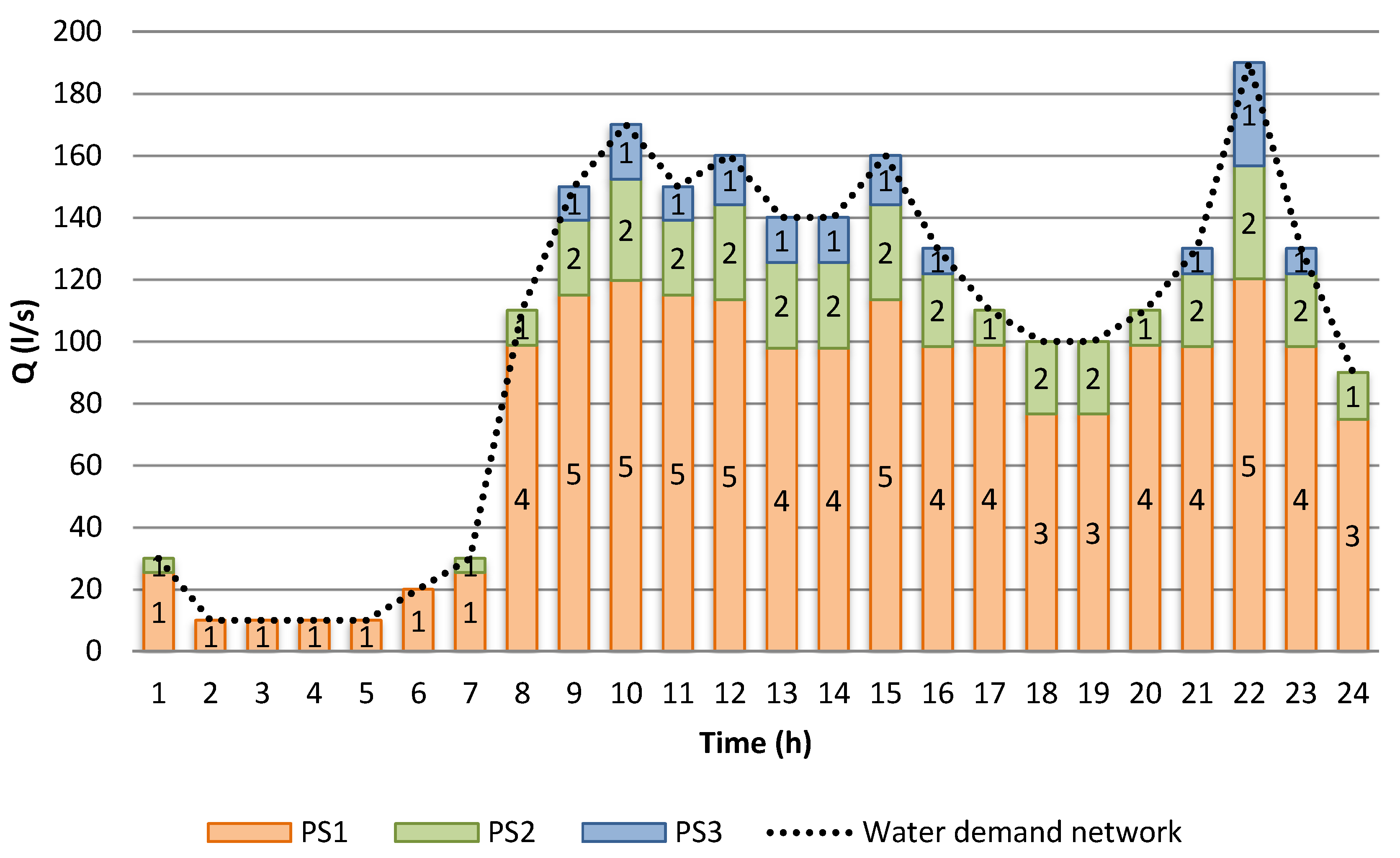
In Table 1, the base demand represents the average or nominal demand for water at the junction. A time pattern is used to characterize time variation in demand, providing multipliers that are applied to the base demand to determine actual demand in a given time period. The demand patterns for the 24 h of a day are presented in Figure 4.

To perform the optimization process, a database with 67 pump models was used. The maximum flow rate of the pumps in the database varied between 9 L/s and 50.7 L/s. The maximum head fluctuated between 15.8 m and 105 m, and the maximum efficiency was in the range of 39% to 84%. The annualized costs of these models were calculated using an interest rate of 5% per year and a projection time of 20 years, as indicated by [7]. This led to an amortization factor F_a = 7.92%. To calculate the length of the pipes (L_p), values of 5, 30, and 10 were used for λ₁, λ₂, and λ₃, respectively.

To calculate CAPEX, the CP₀ and CP₁ values from Equation (10) are 142.88 and 0.5437, respectively, for efficiency values less than or equal to 65% or 203.14 and 0.6115 otherwise. The coefficients of the polynomial equations used to calculate Equation (9) are expressed in the format f(x) = ax² + bx + c. The independent variable (x) can be represented by P or ND. The values of coefficients a, b, and c are shown in

Table 4. Case study coefficients for calculating CAPEX equations.

f(x)	x	a	b	c
Cinv	P(W)	−0.603	116.08	168.19
CSV	ND (mm)	0.01	1.53	11.82
CCV		0.006	0.25	14.55
Cpipe		0.0004	−0.15	8.01
Celbow		0.02	−4.23	269.49
CT		0.001	−1.74	144.24
Cflowmeter		0.051	−7.91	716.64

. These values were determined by [19]. In the case of the pressure transducer (C_pressure) and programmable logic controller (C_PLC), they assume a constant price of 570 and 372.44 EUR, respectively. Furthermore, the flowmeter is always installed in outlet pipe L₃ (Figure 1b) and therefore has the same diameter as that pipe.

2.5. Optimization Method

The proposed optimization model requires the use of a computational method to solve a given problem. The solution space of the problem to be solved in this case study is equal to 10¹⁰⁴ possible combinations, and the objective function is not linear. Therefore, the use of traditional deterministic optimization methodologies is not possible. Because of the huge space of solutions and the complexity of the objective function, it is advisable to use a heuristic method [5]. In the literature, there are many available algorithms that can be adapted to solve the proposed mathematical model. In this case, the meta-heuristic algorithm chosen is a pseudo-genetic algorithm (PGA) developed by the authors, whose details and particularities can be found in [20].

Unlike the traditional version of the genetic algorithm, the PGA is based on the integer coding of its solutions. The software was implemented in the Java language following the specification of [22]. This system can conduct massive simulations and is integrated with the hydraulic network solver EPANET using the programmer’s toolkit [23].

Different parameters guide the search process of the algorithm, so the obtained results are sensitive to the values of these parameters. The main parameters of the proposed PGA are the population size (P), crossover frequency (Pc), and mutation frequency (Pm). We have adopted the optimal parameter calibration range obtained in previous works for the PGA [22,24,25,26]. To ensure a minimum level of statistical confidence of the results, 500 experiments were performed and analyzed.

3. Results

Through the proposed methodology, the designs and operations of the PSs in the case study were optimized.

Table 5. Pump station designs for the case study.

		PS1	PS2	PS3
	ND1	300	200	150
(mm)	ND2	125	125	150
	ND3	300	200	150
	L1	1.5	1	0.75
(m)	L2	3.75	3.75	4.5
	L3	3	2	1.5
	mi	0	0	0
	ni	5	2	1
	H0	38.0800	53.7000	104.9800
	A	−0.02094	−0.06002	−0.04438
	E	0.07130	0.10899	0.05182
	F	0.00167	0.00364	0.00107
	Model Id	GNI 50–16/10	GNI 100–20/50	GNI 50–26/40

details the dimensions of ND₁, ND₂, and ND₃ and the lengths of pipes L₁, L₂, and L₃ according to the modular design presented in Figure 1b. Furthermore, Table 5 shows the number of FSPs and VSPs (m_i, n_i) and the characteristic and efficiency curve coefficients H₀, A, E, and F. In addition, the last row displays the selected model pump from the database.

Figure 5 details the flow ${\mathrm{QS}}_{\mathrm{ij}}$ that must be supplied by ${\mathrm{PS}}_{\mathrm{i}}$ at time step $\mathrm{j}$ according to the calculated setpoint curve. The pattern of daily consumption is represented by a dotted line. Additionally, the number of active pumps is included in the middle of each bar of the graph. If the color associated with a PS does not appear in a bar, it means that it is not necessary to turn on any pumps during that period. The results show that PS1 supplies a large portion of the total flow. However, depending on the required flow and head calculated, the mathematical model determines the optimal combination of active pumps and its speed of rotation to be able to supply exactly the demand of each period.

To clarify,

Table 6. PS designs for the case study.

	PS1				PS2				PS3
T(h)	α	η	QS(L/s)	HS(m)	α	η	QS(L/s)	HS(m)	α	η	QS(L/s)	HS(m)
1	0.714	0.413	25.500	5.773	0.629	0.593	4.500	20.020	-	-	-	-
2	0.436	0.756	10.000	5.137	-	-	-	-	-	-	-	-
3	0.436	0.756	10.000	5.137	-	-	-	-	-	-	-	-
4	0.436	0.756	10.000	5.137	-	-	-	-	-	-	-	-
5	0.436	0.756	10.000	5.137	-	-	-	-	-	-	-	-
6	0.603	0.526	20.000	5.483	-	-	-	-	-	-	-	-
7	0.714	0.413	25.500	5.773	0.629	0.593	4.500	20.020	-	-	-	-
8	0.863	0.671	98.780	15.564	0.706	0.812	11.220	19.231	-	-	-	-
9	0.916	0.736	114.900	20.888	0.782	0.814	24.300	24.011	0.591	0.591	10.800	31.436
10	0.972	0.741	119.765	23.924	0.921	0.787	32.640	29.544	0.694	0.629	17.595	36.784
11	0.916	0.736	114.900	20.888	0.782	0.814	24.300	24.011	0.591	0.591	10.800	31.436
12	0.920	0.741	113.440	21.460	0.885	0.794	30.720	27.944	0.662	0.630	15.840	34.838
13	0.870	0.683	97.790	16.301	0.830	0.804	27.720	25.506	0.631	0.628	14.490	32.491
14	0.870	0.683	97.790	16.301	0.830	0.804	27.720	25.506	0.631	0.628	14.490	32.491
15	0.920	0.741	113.440	21.460	0.885	0.794	30.720	27.944	0.662	0.630	15.840	34.838
16	0.863	0.673	98.410	15.662	0.761	0.814	23.400	22.903	0.552	0.534	8.190	29.053
17	0.863	0.671	98.780	15.564	0.706	0.812	11.220	19.231	-	-	-	-
18	0.809	0.584	76.600	11.240	0.773	0.815	23.400	23.909	-	-	-	-
19	0.809	0.584	76.600	11.240	0.773	0.815	23.400	23.909	-	-	-	-
20	0.863	0.671	98.780	15.564	0.706	0.812	11.220	19.231	-	-	-	-
21	0.863	0.673	98.410	15.662	0.761	0.814	23.400	22.903	0.552	0.534	8.190	29.053
22	1.000	0.748	120.175	25.942	0.992	0.772	36.480	32.888	0.986	0.534	33.345	52.681
23	0.863	0.673	98.410	15.662	0.761	0.814	23.400	22.903	0.552	0.534	8.190	29.053
24	0.793	0.588	74.880	10.901	0.800	0.758	15.120	20.663	-	-	-	-

shows the details of the rotation speed fraction of the pumps (α), used to calculate the efficiency (η) according to Equation (15).

$$\mathsf{\eta }=\mathrm{E}\frac{\mathrm{Q}}{\mathsf{\alpha }\cdot \mathrm{n}}-\mathrm{F}{\left(\frac{\mathrm{Q}}{\mathsf{\alpha }\cdot \mathrm{n}}\right)}^2$$

(15)

where Q is the flow driven by the PS, n is the number of pumps, and E and F are the efficiency curve coefficients. It is important to highlight that, despite the loss of efficiency of the pumps, the level of power consumption in the PSs is the minimum to ensure that all nodes of the network reach the minimum pressure of the network (20 m). The flows Q_ij and heads HS_ij are also presented for each PS_i during a 24 h period.

Table 7. Cost details of the obtained solution.

		PS1	PS2	PS3	Total
CAPEX	Cpump	€ 51,225	€ 20,357	€ 8698	€ 80,280
	Cinv	€ 5024	€ 7274	€ 3108	€ 15,406
	CFacility	€ 16,928	€ 4809	€ 2547	€ 24,284
	CControl	€ 3297	€ 1543	€ 1048	€ 5887
OPEX		€ 19,964	€ 5750	€ 4578	€ 30,292
Fa x CAPEX + OPEX		€ 26,020	€ 8441	€ 5798	€ 40,259

details the CAPEX and OPEX values for the best solution found. First, on the dotted line, all CAPEX terms of Equation (9) are exposed. The OPEX costs are shown according to Equation (13). The last row details the annualized costs according to Equation (2) for each PS. In this case study, the calculated coefficient F_a is 0.0791. The total annualized cost is highlighted in the lower right corner of the table.

Finally, the curve on Figure 6 shows the evolution of objective function value during the process optimization. The best solution is marked by points, while the shaded area represents the represents the solution intervals for the 500 experiments.

4. Discussion

The application of the new methodology aims to find the optimal economic design of PS1, PS2, and PS3, minimizing the sum of CAPEX and OPEX. In addition to the complete design of the PSs, the solution determines the operational conditions of each pump for each time step of the day.

The calculation of the setpoint curve is the key to the methodology presented. By delivering exactly the energy established by the setpoint curve, it is possible to ensure compliance with the predefined head requirements using the minimum amount of energy. This information is then used to design all PSs at once.

The traditional design method takes only the highest point of demand [7]. Consequently, the distribution of flows is considered an isolated optimization stage and does not consider the effects of the operations during the rest of the daily periods. Therefore, the process of finding the lowest cost solution is complex and ineffective. In contrast, the new mathematical model considers the possible energy consumption of WDN operations over the analysis time for each possible design.

In the case study, if only the period with the highest demand is considered (time = 22 h), there are many design combinations for each PS that would allow for the flow rates and heads to be achieved. However, optimizing total costs is not successful. For example, if the pump model selected for PS2 in Table 5 is used for PS1 and PS2, it would be possible to meet the head and flow requirements; however, the total cost would be EUR 50,334. That is, the cost would be 25% more expensive than that of the suggested implementation. In this way, if only the model selected for PS3 is used, the total cost would be EUR 70,980, which represents an increase of 76% compared to the cost of the best solution found. Similarly, the same comparison can be made for all combination options for the 67 models in the database.

The solution obtained indicates that the algorithm did not select any FSP. Although the implementation of VSPs is more expensive and incorporates the loss of efficiency introduced by frequency inverters, these pumps allow for the reduction of excessive energy consumption. Therefore, this turns into lower economic costs. Nevertheless, these results are not generalizable to all networks because the number of pumps in each of them depends on the conditions of each WDN and the current energy prices.

Despite the benefits of the work presented, it does present some limitations. In this work, the control system of pumps fits their heads to a calculated setpoint curve. VSPs are used first, and then FSPs are applied. Therefore, to extend the proposed model, it would be interesting to incorporate other control systems. Additionally, the calculation of OPEX is presented through a second-degree equation; however, the incorporation of a different exponent does not pose a major problem. That is, it does not affect the methodology presented.

5. Conclusions

The design of PSs in a WDN is a very complex and critical problem for any city. Water pumping operations represent a large fraction of the electrical power consumed in urban zones. The investment cost of each PS is very high and directly influences the future energy consumption of the overall network.

Traditionally, this type of design problem is solved by considering only the extreme consumption points or by optimizing the design and operation objectives in two independent stages. This approach does not allow for the capacity of the PS to be adapted to actual operating conditions. Therefore, excess energy is generated, so the costs of WDN grow significantly. To avoid this, a new methodology was proposed in this paper for the design of PSs in networks with multiple pumped water sources and no storage.

A mathematical optimization model was developed to simultaneously minimize the sum of the OPEX and CAPEX incurred by the network through the use of a setpoint curve. Based on the results obtained from the developed model, it is possible to determine the optimal selection of pump models from a database, the numbers of VSPs and FSPs, the lengths and diameters of the pipes, the distribution of flows, and the statuses of the pumps during each period.

A case study was presented, and the results obtained from the application of the PGA were satisfactory. The main benefits of using this new methodology are clearly demonstrable. The use of the setpoint curve ensured compliance with the requests made throughout the WDN and reduced energy excesses by reducing the differences between the consumption curves and the heads used by the pumps. Furthermore, the design of each PS considered the impact of that station on the entire network, including the effects on the rest of the PSs in the long term.

As discussed in the paper, the presented work has some limitations. Only one control system for the pumps is contemplated. That is, VSPs follow the setpoint head, while FSPs only have on/off states. However, the inclusion of new pump control methods does not require any change in the general methodology.

References

1. Mala-Jetmarova, H.; Sultanova, N.; Savic, D. Lost in Optimisation of Water Distribution Systems? A Literature Review of System Design. Water 2018, 10, 307. [Google Scholar] [CrossRef] [Green Version]
2. Şen, Z. Water Structures and Climate Change Impact: A Review. Water Resour. Manag. 2020, 34, 4197–4216. [Google Scholar] [CrossRef]
3. Makaremi, Y.; Haghighi, A.; Ghafouri, H.R. Optimization of Pump Scheduling Program in Water Supply Systems Using a Self-Adaptive NSGA-II; a Review of Theory to Real Application. Water Resour. Manag. 2017, 31, 1283–1304. [Google Scholar] [CrossRef]
4. Gupta, A.; Kulat, K.D. A Selective Literature Review on Leak Management Techniques for Water Distribution System. Water Resour. Manag. 2018, 32, 3247–3269. [Google Scholar] [CrossRef]
5. Mala-Jetmarova, H.; Sultanova, N.; Savic, D. Lost in optimisation of water distribution systems? A literature review of system operation. Environ. Model. Softw. 2017, 93, 209–254. [Google Scholar] [CrossRef] [Green Version]
6. León-Celi, C.; Iglesias-Rey, P.L.; Martinez-Solano, F.J.; Mora-Melia, D. A Methodology for the Optimization of Flow Rate Injection to Looped Water Distribution Networks through Multiple Pumping Stations. Water 2016, 8, 575. [Google Scholar] [CrossRef] [Green Version]
7. Pulido-Calvo, I.; Gutiérrez-Estrada, J.C. Selection and operation of pumping stations of water distribution systems. Environ. Res. J. 2011, 5, 1–20. [Google Scholar]
8. Blinco, L.J.; Simpson, A.R.; Lambert, M.F.; Marchi, A. Comparison of Pumping Regimes for Water Distribution Systems to Minimize Cost and Greenhouse Gases. J. Water Resour. Plan. Manag. 2016, 142, 04016010. [Google Scholar] [CrossRef] [Green Version]
9. Carpitella, S.; Brentan, B.; Montalvo, I.; Izquierdo, J.; Certa, A. Multi-criteria analysis applied to multi-objective optimal pump scheduling in water systems. Water Supply 2019, 19, 2338–2346. [Google Scholar] [CrossRef] [Green Version]
10. Müller, T.M.; Leise, P.; Lorenz, I.-S.; Altherr, L.C.; Pelz, P.F. Optimization and validation of pumping system design and operation for water supply in high-rise buildings. Optim. Eng. 2021, 22, 643–686. [Google Scholar] [CrossRef]
11. Martin-Candilejo, A.; Santillán, D.; Iglesias, A.; Garrote, L. Optimization of the Design of Water Distribution Systems for Variable Pumping Flow Rates. Water 2020, 12, 359. [Google Scholar] [CrossRef] [Green Version]
12. Nguyen, K.D.; Dai, P.D.; Vu, D.Q.; Cuong, B.M.; Tuyen, V.P.; Li, P. A MINLP Model for Optimal Localization of Pumps as Turbines in Water Distribution Systems Considering Power Generation Constraints. Water 2020, 12, 1979. [Google Scholar] [CrossRef]
13. Nagkoulis, N.; Katsifarakis, K. Minimization of Total Pumping Cost from an Aquifer to a Water Tank, Via a Pipe Network. Water Resour. Manag. 2020, 34, 4147–4162. [Google Scholar] [CrossRef]
14. Fecarotta, O.; McNabola, A. Optimal Location of Pump as Turbines (PATs) in Water Distribution Networks to Recover Energy and Reduce Leakage. Water Resour. Manag. 2017, 31, 5043–5059. [Google Scholar] [CrossRef]
15. Shao, Y.; Yu, Y.; Yu, T.; Chu, S.; Liu, X. Leakage Control and Energy Consumption Optimization in the Water Distribution Network Based on Joint Scheduling of Pumps and Valves. Energies 2019, 12, 2969. [Google Scholar] [CrossRef] [Green Version]
16. Weber, J.B.; Lorenz, U. Optimizing booster stations. In Proceedings of the Genetic and Evolutionary Computation Conference Companion; ACM Press: New York, NY, USA, 2017; pp. 1303–1310. [Google Scholar]
17. Kang, D.; Lansey, K. Scenario-Based Robust Optimization of Regional Water and Wastewater Infrastructure. J. Water Resour. Plan. Manag. 2013, 139, 325–338. [Google Scholar] [CrossRef]
18. León-Celi, C.F.; Iglesias-Rey, P.L.; Martínez-Solano, F.J.; Savic, D. Operation of Multiple Pumped-Water Sources with No Storage. J. Water Resour. Plan. Manag. 2018, 144, 04018050. [Google Scholar] [CrossRef]
19. Gil, F.A.A.; Iglesias-Rey, P.L.; Martínez-Solano, F.J.; Cortes, J.V.L.; Mora-Meliá, D. Methodology For Projects Of Pumping Stations Directly Connected To The Network Considering The Operation Strategy. Int. Congr. Proj. Manag. Eng. 2018, 2-018, 551–563. [Google Scholar]
20. Mora-Melia, D.; Iglesias-Rey, P.L.; Martinez-Solano, F.J.; Fuertes-Miquel, V.S. Design of Water Distribution Networks using a Pseudo-Genetic Algorithm and Sensitivity of Genetic Operators. Water Resour. Manag. 2013, 27, 4149–4162. [Google Scholar] [CrossRef]
21. Turci, L.D.O.; Wang, J.; Brahmia, I. Adaptive and Improved Multi-population Based Nature-inspired Optimization Algorithms for Water Pump Station Scheduling. Water Resour. Manag. 2020, 34, 2869–2885. [Google Scholar] [CrossRef]
22. Gutiérrez-Bahamondes, J.H.; Salgueiro, Y.; Silva-Rubio, S.A.; Alsina, M.A.; Mora-Meliá, D.; Fuertes-Miquel, V.S. jHawanet: An Open-Source Project for the Implementation and Assessment of Multi-Objective Evolutionary Algorithms on Water Distribution Networks. Water 2019, 11, 2018. [Google Scholar] [CrossRef] [Green Version]
23. Rossman, L.A. EPANET 2.0 User’s Manual (EPA/600/R-00/057); Water Supply and Water Resources Division, National Risk Management Research Laboratory: Cincinnatti, OH, USA, 2000. [Google Scholar]
24. Mora-Melia, D.; Iglesias-Rey, P.L.; Martinez-Solano, F.J.; Ballesteros-Pérez, P. Efficiency of Evolutionary Algorithms in Water Network Pipe Sizing. Water Resour. Manag. 2015, 29, 4817–4831. [Google Scholar] [CrossRef]
25. Mora-Melià, D.; Martínez-Solano, F.J.; Iglesias-Rey, P.L.; Gutiérrez-Bahamondes, J.H. Population Size Influence on the Efficiency of Evolutionary Algorithms to Design Water Networks. Procedia Eng. 2017, 186, 341–348. [Google Scholar] [CrossRef]
26. Mora-Melià, D.; Iglesias-Rey, P.L.; Fuertes-Miquel, V.S.; Martinez-Solano, F. Comparison of Evolutionary Algorithms for Design of Sewer Systems; CRC Press: Boca Raton, FL, USA, 2009; Volume 1, pp. 261–263. [Google Scholar]
Figure 1. (a) General scheme and (b) PS modular design.
Water 13 03098 g001
Figure 2. Calculation of OPEX and CAPEX.
Water 13 03098 g002
Figure 3. MTF network.
Water 13 03098 g003
Figure 4. Demand pattern for the MTF network.
Water 13 03098 g004
Figure 5. Optimized case study operations.
Water 13 03098 g005
Figure 6. Optimization process evolution.
Water 13 03098 g006