
Assessment of Water Measurements in an Irrigation Canal System Based on Experimental Data and the CFD Model


1
College of Water Resources and Architectural Engineering, Shihezi University, Shihezi 832000, China
2
Shenzhen Water Planning & Design Institute Co., Ltd., Shenzhen 518001, China
*
Authors to whom correspondence should be addressed.
Water 2021, 13(21), 3102; https://doi.org/10.3390/w13213102
Submission received: 22 September 2021
/
Revised: 27 October 2021
/
Accepted: 2 November 2021
/
Published: 4 November 2021
(This article belongs to the Special Issue CFD Modelling of Free Surface Flows)
Abstract
:Due to their convenience, water measuring structures have become an important means of measuring water in irrigation canal systems However, relevant research on upstream and downstream water-depth monitoring point locations is scarce. Our study aims to determine the functional relationship between the locations of the water-depth monitoring points and the opening width of the sluice. We established 14 trunk-channel and branch-channel hydrodynamic models. The locations of the water-depth monitoring points for the upstream and downstream reaches and their hydraulic characteristics were assessed using a numerical simulation and hydraulic test. The results showed that the locations of the upstream and downstream water-depth monitoring points were, respectively, 16.26 and 15.51 times the width of the sluice. The average error between the calculated flow rate and the simulated value was 14.37%; the average error between the flow rates calculated by the modified and the simulated values was 3.36%. To further verify the accuracy of the modified discharge calculation formula, by comparing the measured values, we reduced the average error of the modified formula by 19.29% compared with the standard formula. This research provides new insights into optimizing water measurements in irrigation canal systems. The results provide an engineering basis for the site selection of water-depth monitoring points that is suitable to be widely applied in the field.
1. Introduction
Real-time monitoring of the diameter in the irrigation area plays an important role in improving water management and reasonably allocating water consumption. This type of monitoring is a common method used to calculate the discharge rate in an open channel by converting the upstream and downstream water depths of the plate sluice [1,2]. Fluctuations in the water surface can produce errors in observations of upstream and downstream water depths which will ultimately affect the calculation of the discharge rate. Therefore, the correct location of the water-level reading is of great significance for accurately calculating the flow rate. At present, there are no specific recommendations for the locations of water-depth monitoring points in many standard specifications; previous research on water surfaces mainly applied classical hydraulic theory and numerical simulations [3].
The improvement of computer performance has greatly promoted the development of computational fluid dynamics (CFD), and many scholars have performed in-depth research on the hydraulic characteristics of open channels by using the CFD software package [4]. Cornelius et al. [5] presented an algorithm for calculating flow rate based on the hydraulic structure and the slope–hydraulic radius method; by comparing the measured fluid depth with the simulated depth based on the one-dimensional Saint Venant equation, the authors obtained the flow-rate model adjustment parameters. The results showed that the error of flow measurements in the Venturi flume decreased from 2.3% to 0.8%. Marcela et al. [6,7,8] used the Lagrangian–Eulerian finite element analysis method to calculate the free surface flow. This method was applied to a test in a laminar flow over a broad-crested weir and used to investigate the velocity profile at the inlet and outlet, in addition to a temporal evolution of the free surface at the exit of the broad-crested weir. Maronnier et al. [9] established a numerical model for solving complex flows with free surfaces and computed the position of the free surface in a volume fraction of liquid by using the splitting algorithm method to decouple advection and diffusion phenomena. The numerical results showed the efficiency of the proposed method and were in good agreement with the experimental results. Meselhe et al. [10] presented a two-step, predictor–corrector, implicit numerical scheme for simulating transcritical flows; the results showed that the proposed scheme is robust and accurate and can accurately simulate hydraulic water-measuring structures.
The research method for numerical simulation combined with hydraulic testing provides a theoretical basis for the study of hydraulic characteristics and engineering applications. Different ideas have been put forward for research in the field of water conservancy engineering technology [11,12].
Omid et al. [13] numerically simulated and analyzed the air–water two-phase flow in a curved 30° open-channel bend and compared the results with those of a 90° curve. The intensity of the helical motion of fluid particles depends on the shape of the open channel. Although the secondary flow was not intense in the 30° bend model, the tendency toward flow separation was noticeable. Mariana et al. [14] researched the velocity variation in a pump as a turbine system with a specific speed and conducted experiments and CFD simulations; the authors optimized the shape of the impeller by studying the flow velocity distribution under different discharge values and rotational speeds. Ali et al. [15] numerically studied the flow around a triangular labyrinth side weir with three different angles (45, 60, and 90°). The discharge values for the labyrinth side weir were 1.7, 1.33, and 1.25 times those of the normal side weir, respectively. The vortices were strongest at 45°. Through three cases (single-phase water flow over a ground sill, free surface flow over a hill, and complex free surface flow in a sewer model), Katharina et al. [16] evaluated the accuracy and applicability of three RANS turbulence models: k-epsilon, k-omega, and k-omega SST. In general, the results of the standard k-epsilon turbulence model at all positions were slightly better than the results of the other RANS models. Jahanbakhsh et al. [17] developed CICSAM (compressive interface capturing scheme for arbitrary meshes). CICSAM is a discretization scheme to circumvent the problems associated with the advection of a step profile across Eulerian meshes. This scheme was based on the solution of a transport equation for a fluid-indicator function chosen to be the volume fraction. This study applieded interpolation for the volume-fraction transport equation, the fractional step method for velocity, and the pressure-coupling finite-volume solver and validated the calculations for two-dimensional and three-dimensional test cases (sloshing of a liquid wave and dam breaking). Shahrouz et al. [18,19] presented a numerical method for a two-phase flow to model an incompressible liquid interacting with a compressible gas and used the volume of fluid (VOF) method to describe the liquid–gas free interface. To obtain a more accurate approximation of the interface, a novel adaptive Eulerian grid subdivision method was defined. The results showed that the adaptive Eulerian grid refinements are optimized to efficiently reduce numerical diffusion. Ramamurthy et al. [20,21,22] applied RANS equations to flow past a floor slot, adopted the two-dimensional two-equation k-ω turbulence model for the numerical simulation, and used the VOF method for treating free surfaces to obtain the pressure-head distribution, velocity distribution, and water surface profile, respectively. These flow parameters were in good agreement with the experimental data, and this model was able to properly predict the flow characteristics under various actual flow conditions. Muste et al. [23,24] studied the hydraulic characteristics of flow velocity and turbulence in open channels with and without sediment. The research results showed that the size of the sediment particles can affect turbulence intensity. With the addition of sediment, the fluctuations in water velocity did not change, but the sediment was reduced.
While most research has focused on the development and application of advanced water-measuring equipment and hydraulic performance, the detailed processes of the installation and management of water-measuring equipment have been rarely studied. Numerical simulation can accurately predict the development laws of water flow. The VOF method is an important method used to study the free surface flow in open channels and has attracted considerable attention in recent decades [25,26].
We chose the Heping Irrigation District in Northeast China as an example and used the methods of numerical simulation and hydraulic testing to determine the specific location for measuring the depth of the channel. We also modified the flow coefficient of the flow calculation formula to improve the accuracy of flow measurements. This work is meaningful for research on water surface profile and the hydraulic characteristics of open channels and provides a theoretical basis for the operation of irrigation-district management manuals.
2. Materials and Methods
2.1. Hydraulic Test
2.1.1. Overview of Study Area
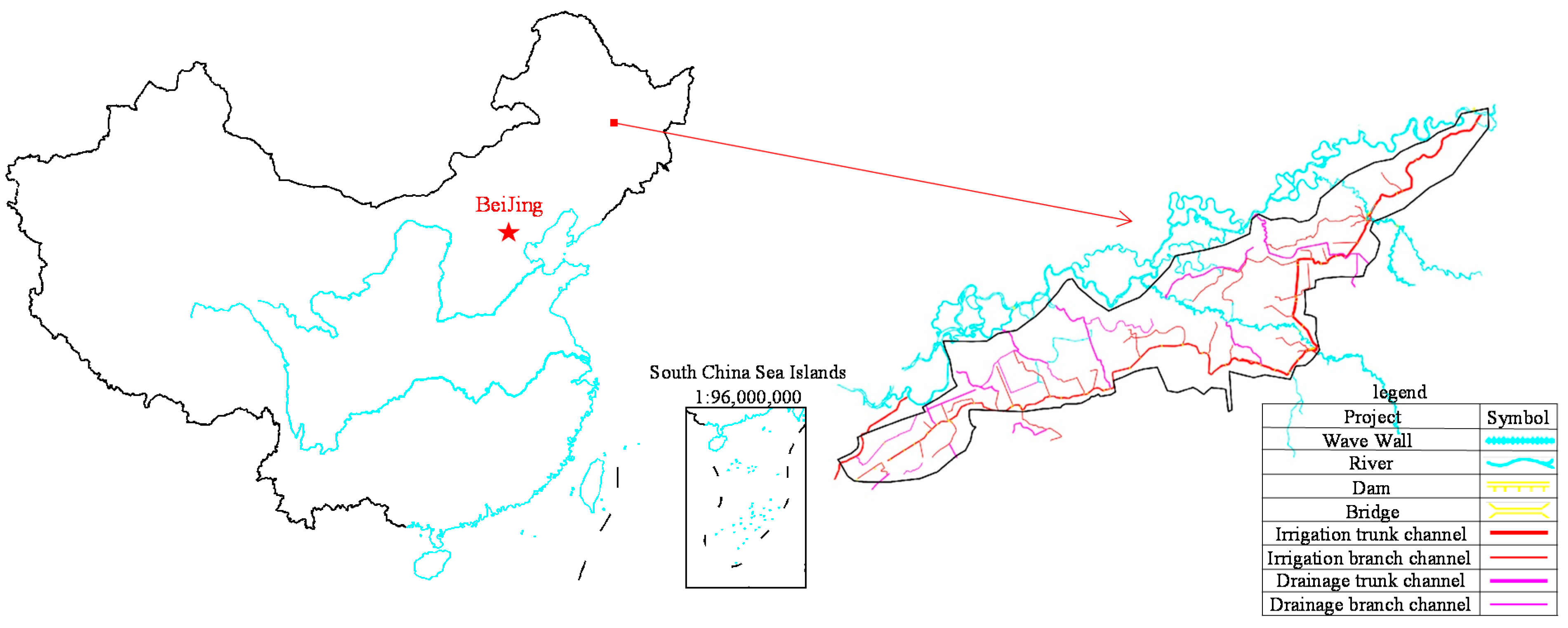
Heping Irrigation District (125°55′ E to 128°43′ E, 45°52′ N to 48°03′ N) is located in Qing′an County, Heilongjiang Province, China, and belongs to the junction of the Songnen Plain and the Lesser Khingan Mountains. The irrigated area covers 375.2 km2, including a trunk channel with a length of 45 km and a roughness factor of 0.017, 22 branch channels with a total length of 60 km, and 16 drainage trunk channels with a total length of 50.84 km (Figure 1).
2.1.2. Field Test Layout
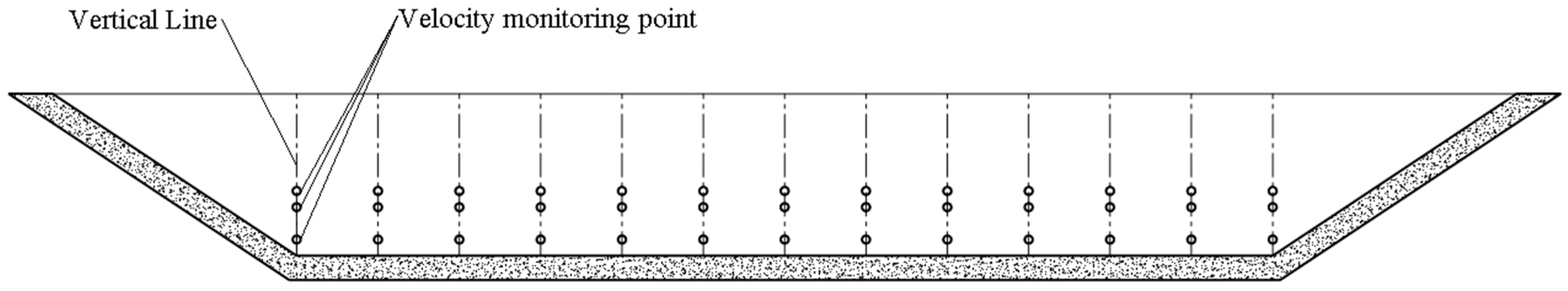
The irrigation canal system in this study was composed of a trunk channel and a branch channel. The section forms and relative elevation between the trunk channel and branch channel are shown in Table 1. According to the water measurement specifications for irrigation channel systems [27,28], 13 vertical lines were arranged on the trunk-channel section, and 3 measuring points were arranged on each vertical line to measure the velocity and discharge of the trunk-channel and branch-channel sections (Figure 2). Other branch channels used the corresponding vertical-line and measuring-point arrangement measures according to the actual situation and the standard specifications.
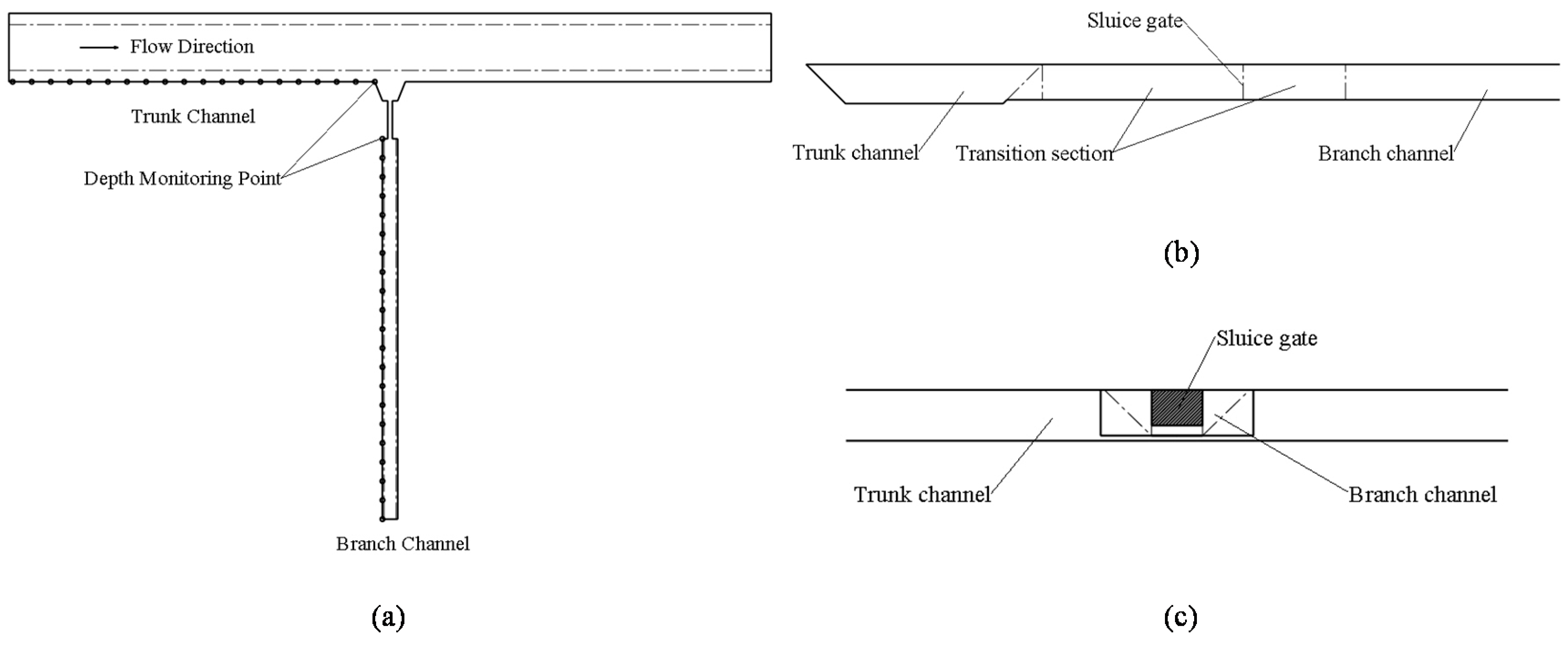
For field measurements of the hydrologic features of trunk and branch channels in Heping Irrigation District, the water depth, channel section velocity, and elevation of the trunk and branch channels were measured using an LS-10B propeller-type current meter, water gauge, and leveling gauge. Taking the position of the sluice as the reference point, a monitoring point was arranged every 5 m within 100 m of the upstream of the trunk channel to record the changes in water depth; monitoring points were also placed downstream of the branch channel and upstream of the trunk channel, as shown in Figure 3. The sluice opening was defined as the ratio of the sluice opening height to the height of the sluice.
2.2. Numerical Simulation Test
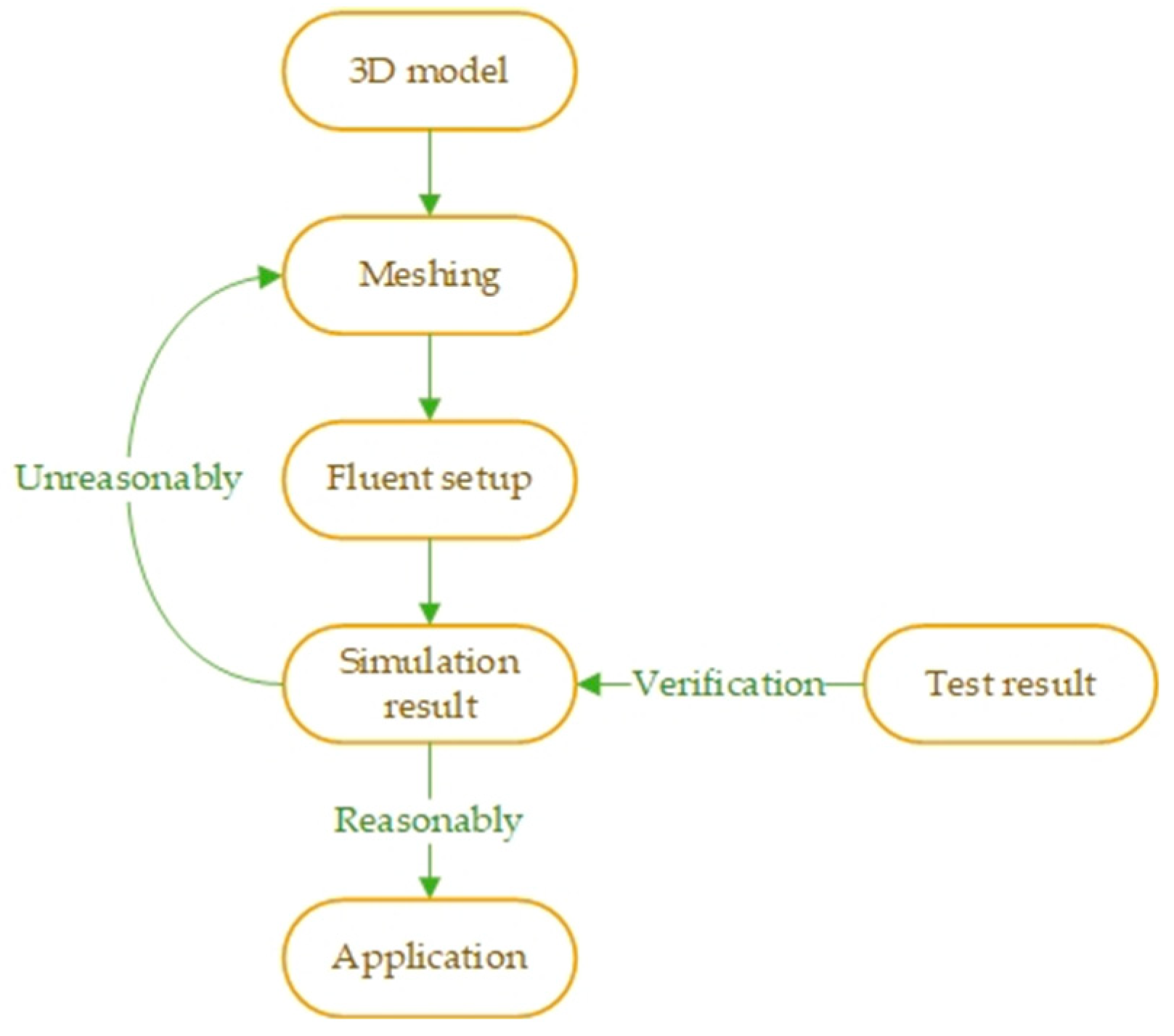
Numerical simulation calculations were carried out on the three-dimensional physical model of the channel and verified through testing to obtain reasonable modeling results and carry out field applications. A flowchart of the test process for the numerical simulation is provided in Figure 4.
2.2.1. Control Equation
The continuity equation and momentum equation for open-channel free incompressible fluid can be expressed as [29]
where is the flow velocity, m/s; u, v, and w are, respectively, the velocity components of fluid particles in the three-dimensional spatial directions x, y, and z, m/s; ρ is the density of water, kg/m3; μ is the dynamic viscosity, N·s/m2; p is the pressure, Pa; and Fu, Fv, and Fw are the forces of fluid particles in the three-dimensional directions x, y, and z, N/m3.
2.2.2. Turbulence Models
The RNG k-ε turbulence model solves the problems of rotation and swirling in the average flow by correcting the turbulent viscosity, enabling the model to correctly handle the situation where the open-channel flow is divided into the branch channel and the streamline is bent [30]. This model offers high accuracy for solving such problems, and the equation is expressed as
where k is the turbulent kinetic energy, m2/s2; ε is the turbulent energy dissipation rate, kg·m2/s2; μ is the hydrodynamic viscosity coefficient, N·s/m−2; Gk is the turbulent kinetic energy production term, ; μeff is the effective dynamic viscosity coefficient, N·s/m−2; C1ε is the constant 1.42; and C2ε is the constant 1.68.
2.2.3. VOF Method
The problem of channel free surface fluctuations involves the two phases of air and water. The VOF model has good applicability when dealing with a variety of disjointed interfaces [31] and can simulate two or more immiscible fluids by solving a single momentum equation and tracking the volume fraction of each fluid in the computational domain. The VOF model can also be reasonably applied to the movement of bubbles, the flow of water in dam break, and the tracking of the free surface of an open channel. In each control body, the sum of the volume fractions of all phases is 1:
where aw and aa are, respectively, the volume fractions of water and air in each control unit in the calculation domain (when aw = 1, the control volume is completely filled with water; when aa = 1, the control volume is completely filled with air).
aw + aa = 1
The water–air interface is tracked using a continuity equation, which is expressed as
where ui is the velocity component, m/s, and xi is the coordinate component.
2.2.4. Meshing and Irrelevance Analysis
The three-dimensional irrigation canal system of the trunk and branch channels was designed using the SolidWorks 2014 software (Dassault Systèmes, Concord, Dassault Systems, Concord, CA, USA), and the ICEM CFD 18.0 software (ANSYS, Inc., Pittsburgh, PA, USA) was applied to mesh the physical model. Compared to unstructured grids, structured grids have the advantages of more regular grid shape and node distributions and better grid quality. In our study, a hexahedral structural grid was used to mesh the physical model. To better simulate the flow characteristics of the water flow near the wall, the wall grid was completely dense from bottom to top. In order to explore the effects of the grid-cell size on the accuracy of the numerical simulation results, five different methods were used to mesh the first branch-channel physical model (the maximum grid cells were 0.8, 0.9, 1.0, 1.1, and 1.2 mm). We set the inlet depth of the trunk channel to 1.20 m and the flow velocity to 0.6753 m/s (please refer to Section 2.2.5 for the boundary conditions and calculation model settings). We then performed numerical simulation calculations. Based on the water depth at the outlet of the branch channel, when the water depth no longer changed with the densification of the grid, the meshing method was considered to represent an optimal scheme. As shown in the relationship between the mesh size and the depth of the outlet branch channel in Table 2, when the maximum mesh size was less than 0.9 mm, there was no substantial change in the downstream water depth, thus dividing the standard mesh as in other branch channels (see Figure 5).
2.2.5. Numerical Simulation Method
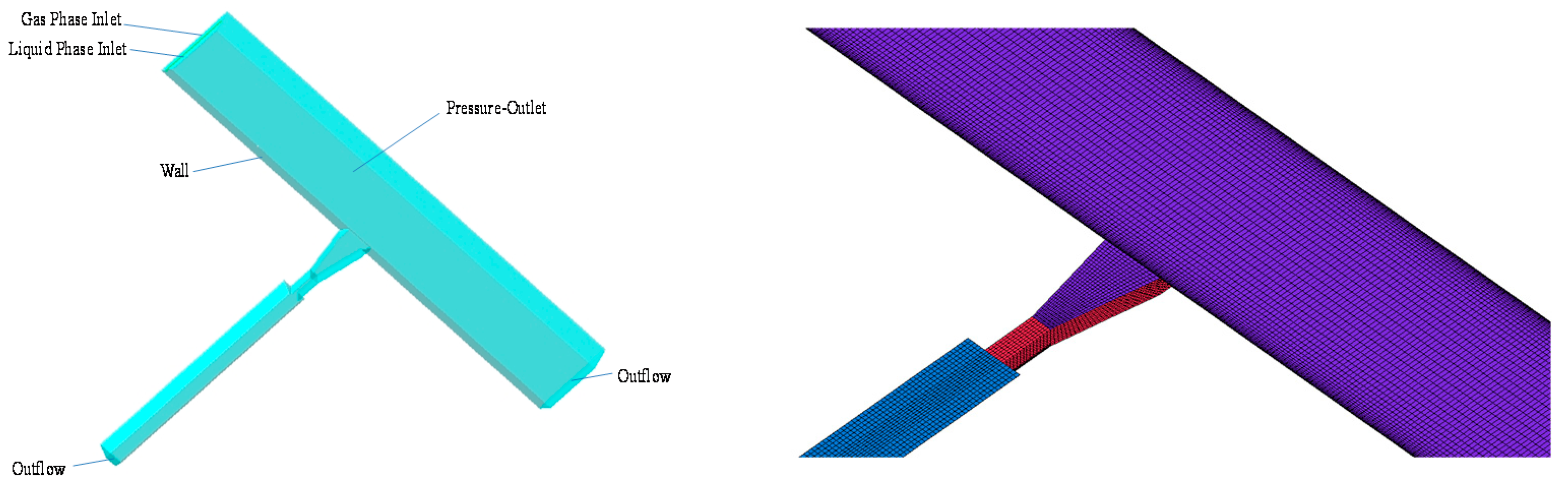
We set the trunk-channel inlet flow to 11.1829 m3/s (the design flow value of the trunk channel). The inlets were set to the gas phase and liquid phase. The air phase adopted the pressure inlet and default standard atmospheric pressure, while the water phase adopted the velocity inlet; the inlet flow rate was set to 0.6753 m/s. The turbulence intensity was 5%; the hydraulic diameter was 1.0143 m; the outlets of the trunk and branch channels were set to free flow; the wall was set as a standard nonslip wall; and the opening degrees of the sluice were 0.1, 0.2, 0.3, 0.4, 0.6, 0.8, and 1.0.
The calculation model was based on the pressure method, the VOF method, and the RNG k-ε models, and we set the gravity to 9.81 m/s2. The basic governing equation was the N-S equation. We adopted first-order upwind style discretization and the PISO algorithm for flow field calculation. We set the initial value of the water phase in the calculation domain to 0 and initialized it. We marked the water volume of the downstream channel to reflect actual submergence conditions with a 0.001 residual convergence value and used an iteration number of 20,000 steps.
2.2.6. Model Rationality Verification
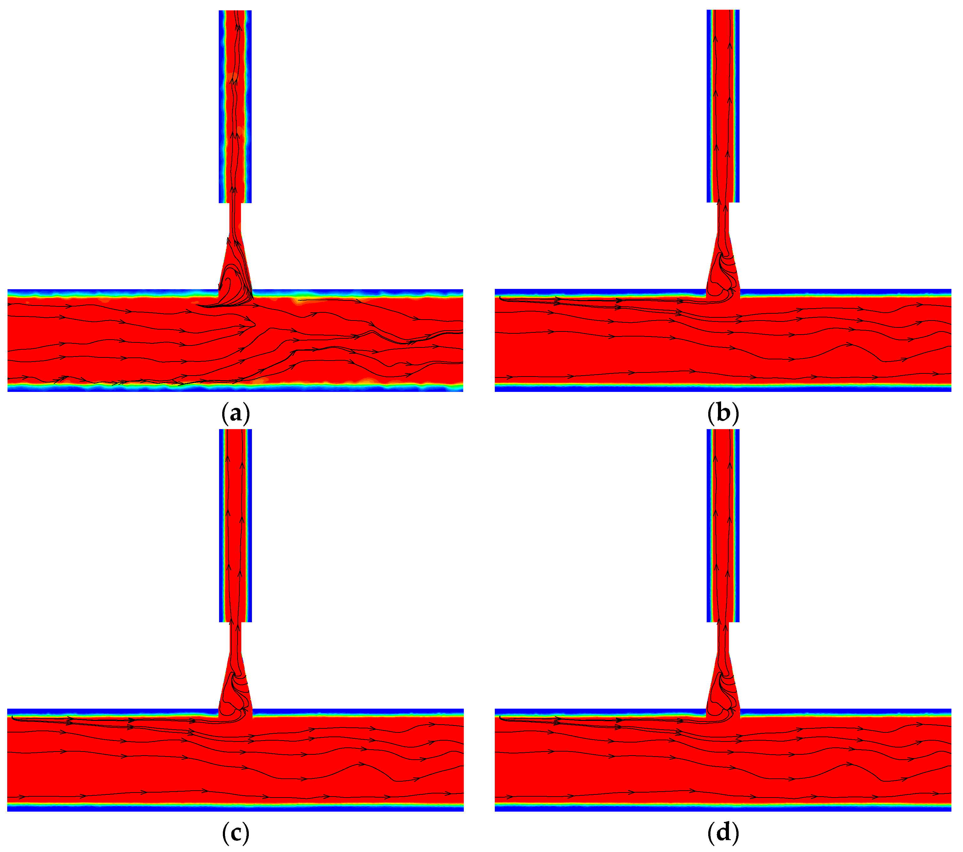
To determine whether the numerical calculation model could fulfill the applications of the trunk-channel and branch-channel water-delivery system, the numerical simulation result of the fourth branch channel were compared to those of the field-test data. The results for the numerical simulation of the water surface and streamline distribution of the fourth branch channel during sluice opening were 0.2, 0.4, 0.6, and 0.8, as shown in Figure 6. A comparison of the experimental flow values and the simulated flow values is provided in Table 3. The average errors for the numerical and experimental values of the trunk-channel inlet flow rate and the branch-channel outlet flow rate were, respectively, 3.067% and 3.579%; the average errors for the numerical and experimental values of the trunk-channel inlet water depth and the branch-channel outlet water depth were, respectively, 2.363% and 2.9%. The results showed that the VOF method can accurately simulate the profile of the water surface and that the numerical results can truly reflect the hydraulic characteristics and real flow conditions of the trunk-channel and branch-channel water-delivery system, as well as meeting the relevant testing requirements.
3. Results
3.1. Engineering Applications of the Numerical Simulation
We established a numerical model for the hydrodynamics of 14 channels in the irrigation area and obtained numerical simulation results under different working conditions. The VOF method and the RNG k-ε turbulence model can accurately handle the streamline bending and swirling conditions of open-channel water flow. The structured grid is suitable for dividing geometric bodies with regular shapes and makes it easy to realize the fit of the boundary area. Comprehensive analysis of the numerical simulation and experimental data showed that the average error between the two was 2.978%. Numerical simulation methods have the advantages of strong adaptability, wide applications, and short test periods and represent an effective technique for engineering research.
3.2. Water Surface Numerical Results
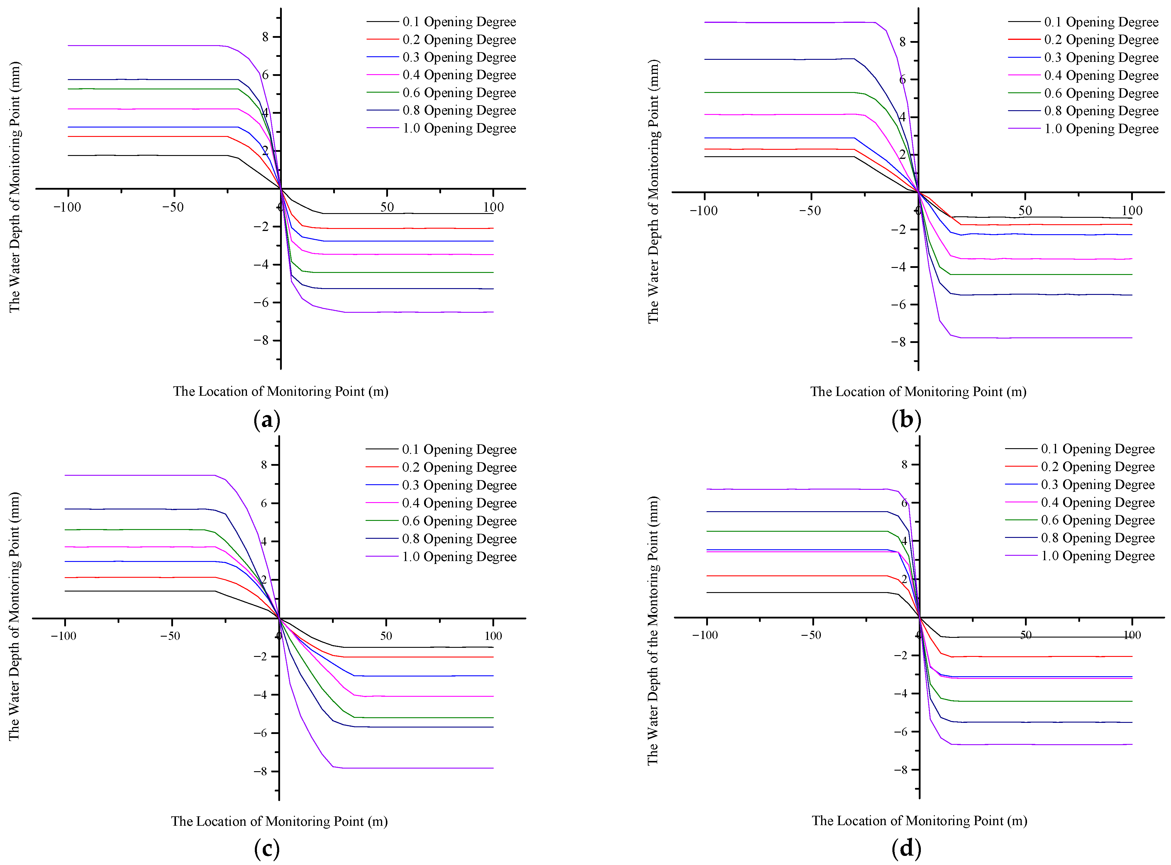
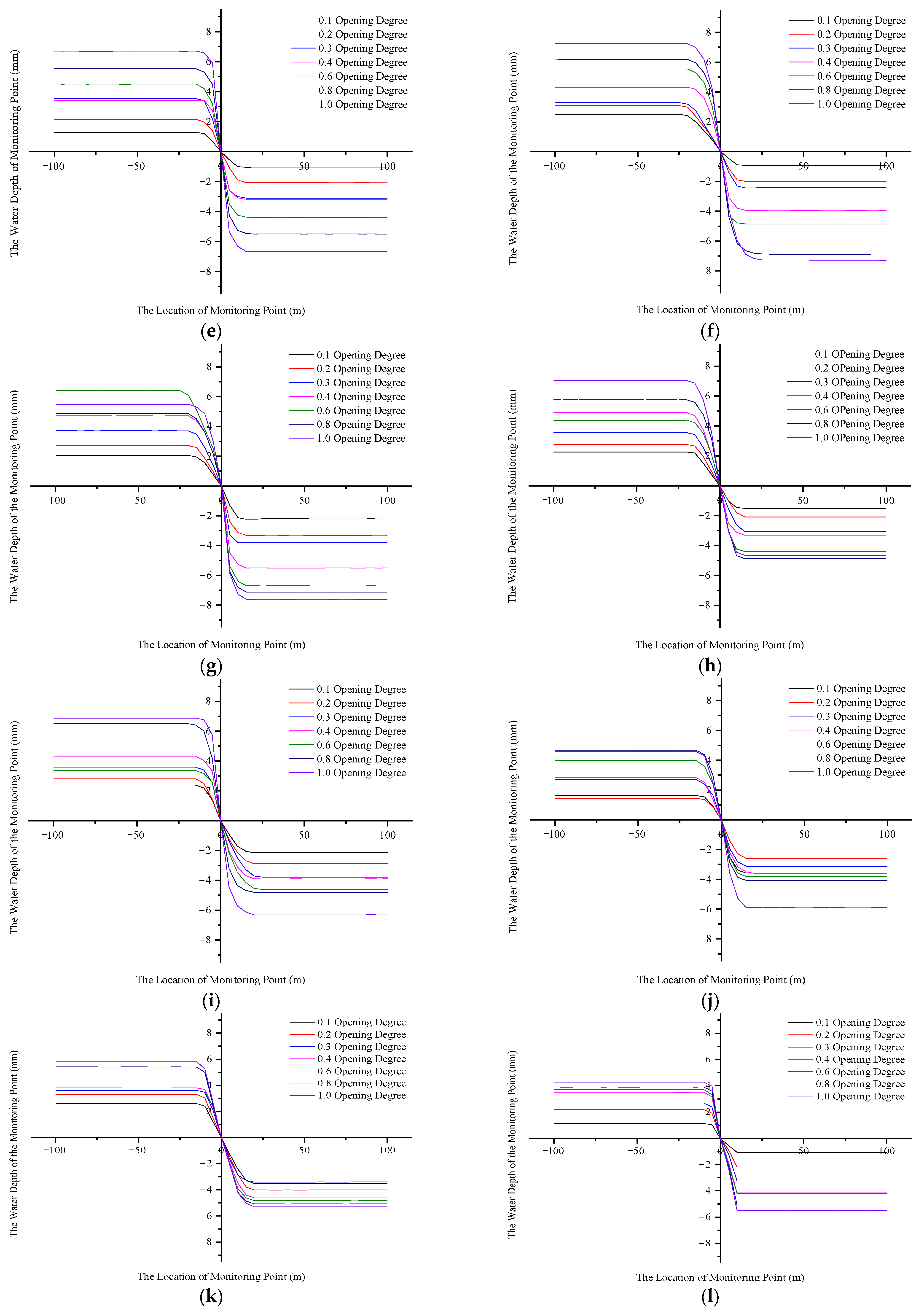
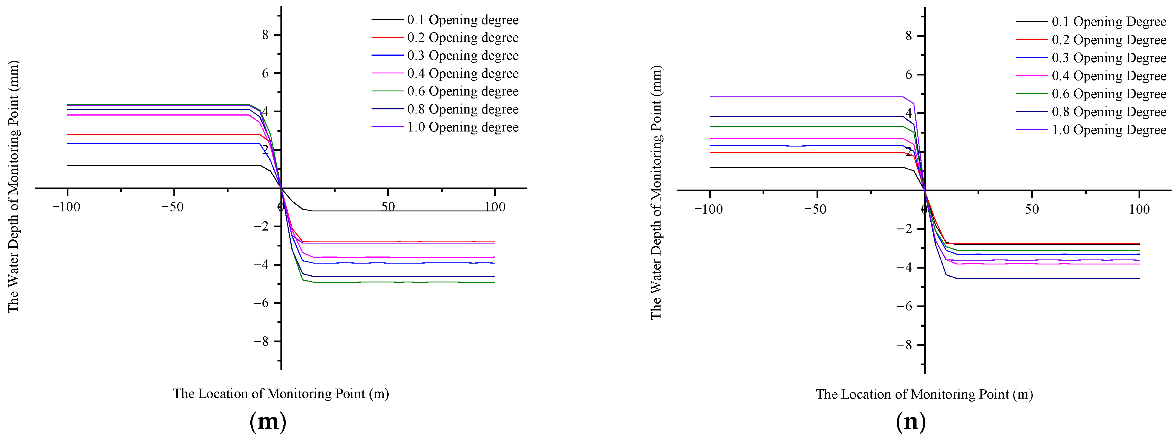
To explore the area where the water surface is stable and use this area as the location of the water-level monitoring point, we applied the Fluent 18.0 software to derive the abscissa and ordinate of the water–air interface of the longitudinal section of the trunk channel and the branch channel and draw the relationship between the position of the monitoring point and the fluctuation of the water-surface line, as shown in Figure 7. To describe the change law of the water surface more intuitively, the water depth at the sluice was taken as the zero point. The slope of the curve indicates the trend of water depth changes, and the water surface is in a stable state when the curve is horizontal. The inflection point of the curve was used as the criterion for evaluating the stability of the liquid level and as the location for measuring the depth of the channel.
In Figure 7, the turning point indicates that the water-surface line was stable at a certain distance from the sluice to the upstream of the trunk channel and the downstream of the branch channel. The 14th branch channel showed a similar pattern from the 1st to 17th branch: The water depth remained stable after the upstream and downstream water levels receded from the gate by a certain distance, and the water surface fluctuated little. Due to the branch channel′s diversion from the trunk channel, the flow state of the trunk channel was affected by the drag force generated from the branch canal′s diversion, resulting in a larger curvature of the streamline at the intersection of the main stream and tributary. The water flow in the area near the sluice was subject to the action of external forces such as lateral pressure, shear force, and centrifugal force, resulting in a vortex zone and a backflow zone and aggravating the flow disturbance. In the area far from the sluice, the external force of the water flow was less, and the water surface tended to be stable. We used the location with a relatively stable water surface for the water-level reading and fitted the function to the width of the sluice. Table 4 shows the functional relationship between the positions of the upstream and downstream water-level monitoring points and the sluice width.
The correlation function coefficients of the 14 branch channel were then weighted and averaged to obtain the functional correlation expressions for the entire Heping Irrigation District. The average value was used as the basis for determining the position to measure the depth of the trunk and branch channels.
3.3. Flow Formula Calibration
In the water measurement specifications for irrigation canal systems, the formula for calculating the flow rate of a rectangular single-hole sluice can be expressed as [27,28]
where Q is the discharge, m3/s; μ is the discharge coefficient, 0.64; hg is the height of the sluice opening, m; H is the upstream water depth, m; b is the sluice width, m; g is the gravity acceleration, 9.81 m/s2; and ZH is the water-level difference between upstream and downstream, m.
Q = μ(1 + (0.65 hg/H))bhg(2 gZH)0.5
The flow rate was calculated based on the upstream and downstream water depths and the opening of the sluice, without considering the existence of the branch channel. Therefore, the value of the discharge coefficient μ was modified in the flow calculation formula to conform to the actual situation of Heping Irrigation District.
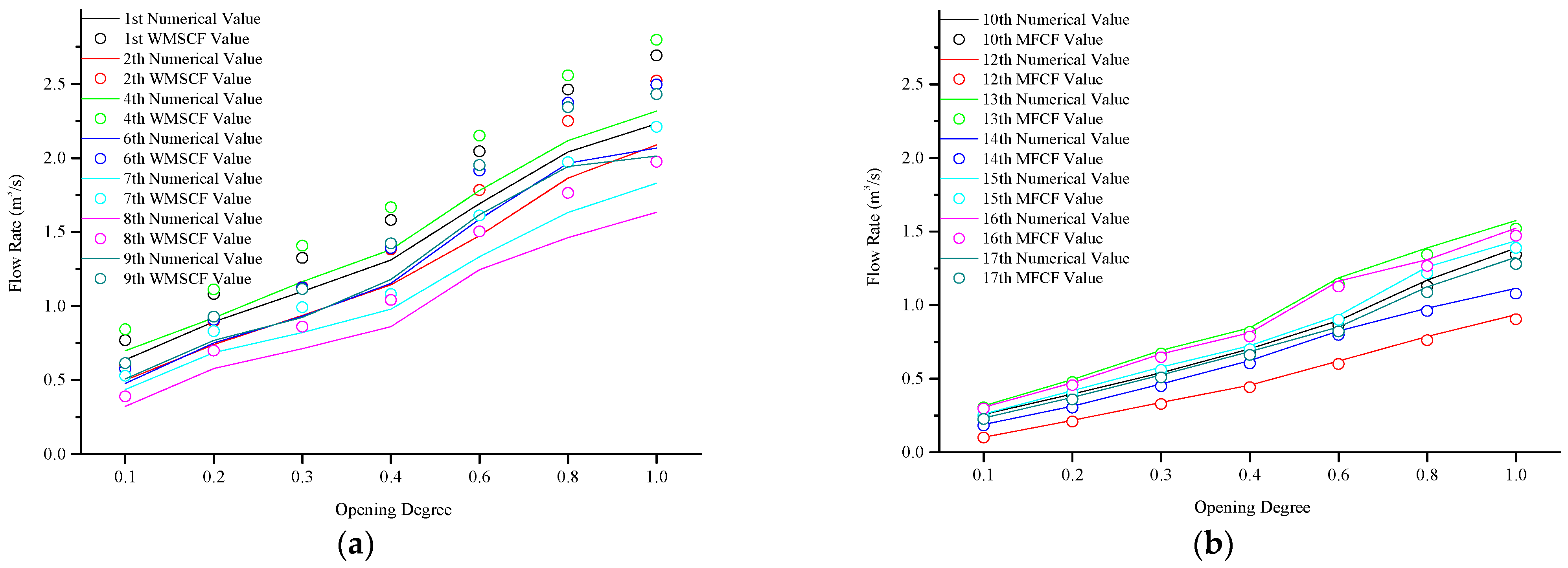
In this study, the flow rates of seven branch channels (first to ninth) were calculated using the standard calculation formula for water measurements in irrigation canal systems and compared to numerical data to analyze the errors. As shown in Figure 8a, the absolute error between the flow rate calculated by the calculation formula for water measurement specifications and the numerical data was 17.218% at maximum and 9.528% at minimum. This study then used the modified flow calculation formula to calculate the flow values of the remaining seven branch channels (10th to 17th). As shown in Figure 8b, the absolute error between the flow rate calculated by the modified flow calculation formula and the numerical data was 4.096% at maximum and 3.444% at minimum.
By using the SPSS software and refitting the correlation between Q, μ, hg, H, b, and ZH, the discharge coefficient μ (0.64) was corrected to μ′, and its value was determined to be 0.53.
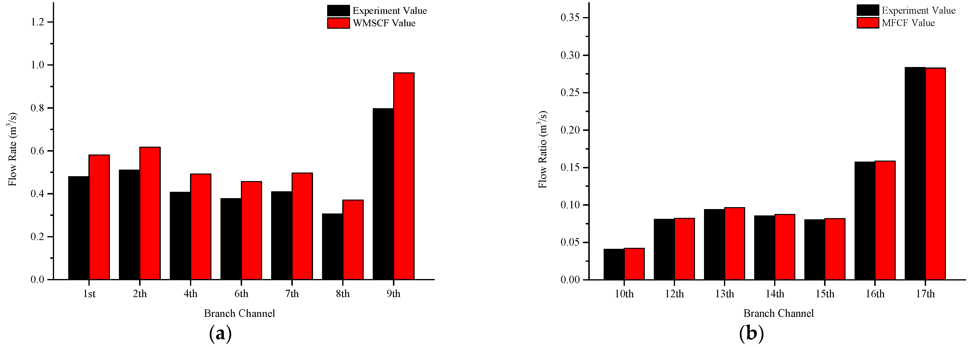
To verify the accuracy of the modified flow calculation formula, we used the calculation formula for water measurement specifications to calculate the discharge of seven branch channels (first to ninth) and compared the results to experimental data. As shown in Figure 9a, the error between the flow rate calculated by the calculation formula for water measurement specifications and the experimental data was 21%. We next used the modified flow calculation formula to calculate the flow values of the seven remaining branch channels (10th to the 17th). As shown in Figure 9b, the average error between the flow rate calculated by the modified flow calculation formula and the numerical data was 1.71%. The results showed that by modifying the value of the flow coefficient μ′, the error range of the flow measurement accuracy can be controlled within 5%.
4. Discussion
At present, the primary method of researching the hydraulic characteristics of open channels involves a combination of numerical simulations and hydraulic tests. Based on the irrigation canal system of the 14 trunk and branch channels in Heping Irrigation District, this study proposed a hydrodynamic model for numerical simulations to explore the position of the water-level monitoring point and provide a fitting flow calculation formula.
In this work, a numerical simulation and hydraulic test were carried out based on the hydraulic characteristics of the open channel. The average error between the numerical values and experimental results of water depth and flow at the trunk-channel inlets and branch-channel outlets was 2.978%, which shows that the calculation method in the CFD software package is reliable. Therefore, this method can be used to study open channels in irrigation canal systems. The numerical results showed that the locations of the upstream and downstream water-depth monitoring points were 16.26 and 15.51 times the width of the sluice, respectively; these values were proposed for the first time in this research. After consulting a large number of domestic and foreign specifications for water measurements of irrigation canal systems along with irrigation district management manuals, Bos et al. [27,28] suggested only that the location of the water level′s monitoring point should be a channel section with a regular cross-section, stable water flow, and no siltation at the bottom of the canal. No clear value requirements were reported.
The specifications for water measurements of irrigation canal systems are not suitable for flow calculations of channels with branch canals. It was thus necessary to refit the flow coefficient μ in the flow calculation formula to obtain a flow calculation formula suitable for the actual situation of Heping Irrigation District. The results of refitting the flow calculation formula and verifying the formula with actual measured values showed that the error of flow measurement decreased from 21% to 1.71% and that the refitted flow calculation formula has good applicability.
To further improve water management and water conservancy planning and design in irrigation districts, some issues remain to be studied:
- There are different degrees of sedimentation and siltation in actual channel water flow. In the data monitoring, we explored whether the different degrees of siltation would affect the distribution law of the water-surface line.
- The Froude number and Reynolds number will also have an impact on changes in the hydraulic performance of water flow. In the future, the effects of different Reynolds numbers and Froude numbers on hydraulic performance, such as head loss and changes in turbulent kinetic energy, should be studied.
In the present study, we analyzed the hydraulic performance of open channels based on the water surface profile and flow measurement accuracy, and we provided a theoretical basis for the site selection of water-depth monitoring points. Future studies could pursue the automation and digitization of water-regime monitoring in irrigation areas through sensor monitoring of water depth, the Internet of Things, cloud computing, and terminal equipment. These developments would comprehensively enhance the construction and development of modernized irrigation districts.
5. Conclusions
In this work, water measurement of irrigation canal systems was studied using numerical simulation analysis and field monitoring for an open-channel water surface. The maximum absolute error between the simulated flow value and the test value was 3.69%, and the minimum was 3.56%; the maximum absolute error between the simulated water depth value and the test value was 2.74%, and the minimum was 0.493%. The numerical model of hydrodynamics was found to be reasonable and could provide a theoretical reference for exploring and optimizing water measurements and open-channel hydraulic performance in the irrigation district. The 14 trunk-channel and branch-channel models constructed in the CFD software showed that, when using the RNG k-ε model, the numerical calculation model of the VOF method offers higher simulation accuracy for the open-channel water surfaces. By refitting the flow coefficient, the accuracy of flow measurement was also significantly improved. The method proposed in this work was applied to 14 channels in the Heping Irrigation District of Northeast China, and the results showed that using the modified flow calculation formula to calculate the flow rate provides significant improvements in the accuracy of flow measurements.
Author Contributions
Z.W. and W.L. provided the idea of the study and writing of the manuscript; H.X. conducted simulation test and data analysis; Q.W. provided important advice on the concept of the methodology. All authors have read and agreed to the published version of the manuscript.
Funding
This work was supported by the Innovation Team Project in Key Fields of Xinjiang Production and Construction Corps (XPCC) (2019CB004) and Southern Xinjiang Key Industry Innovation and Development Support Plan Project of Xinjiang Production and Construction Corps (XPCC) (202DB004).
Institutional Review Board Statement
Not applicable.
Informed Consent Statement
Not applicable.
Data Availability Statement
The data that support the finding of this study are available from the corresponding author upon reasonable request.
Acknowledgments
We sincerely thank the College of Water Resources and Architectural Engineering (Shihezi University) for providing the experimental site.
Conflicts of Interest
The funders had no role in the design of the study; in the collection, analyses, or interpretation of data; in the writing of the manuscript; or in the decision to publish the results.
References
- Stock, E.M. Methods of Measurement of Irrigation Water, 1st ed.; Utah State Engineering Experiment Station and Utah Cooperative Extension Service, Utah State University: Logan, UT, USA, 1955; pp. 13–15. [Google Scholar]
- Wubbo, B. Flow measurement structures. Flow Meas. Instrum. 2002, 13, 203–207. [Google Scholar]
- Szymkiewicz, R. Numerical Modeling in Open Channel Hydraulics, 1st ed.; A&M University: College Station, TX, USA, 2011; pp. 111–157. [Google Scholar]
- Marcela, C.; Laura, B.; Mario, S.; Jorge, D. Numerical Modeling and Experimental Validation of Free Surface Flow Problems. Arch. Comput. Methods Eng. 2016, 23, 139–169. [Google Scholar]
- Cornelius, E.A.; Asmund, H.; Geir, E.; Bernt, L. Algorithm with improved accuracy for real-time measurement of flow rate in open channel systems. Flow Meas. Instrum. 2017, 57, 20–27. [Google Scholar]
- Marcela, C.; Diego, C.; Piotr, B.; Pierre, V.; Alain, R. A surface remeshing technique for a Lagrangian description of 3D two-fluid flow problems. Int. J. Numer. Methods Fluids 2009, 63, 415–430. [Google Scholar]
- Henning, B.; Peter, W. Arbitrary Lagrangian Eulerian finite element analysis of free surface flow. Comput. Methods Appl. Mech. Eng. 2000, 190, 95–109. [Google Scholar]
- Nasser, A.; Tiberiu, B.; Gang, W. A computational Lagrangian-Eulerian advection remap for free surface flows. Int. J. Numer. Methods Fluids 2010, 44, 1–32. [Google Scholar]
- Maronnier, V.; Picasso, M.; Rappaz, J. Numerical simulation of free surface flows. J. Comput. Phys. 1999, 155, 439–455. [Google Scholar] [CrossRef]
- Meselhe, E.A.; Holly, F.M. Numerical Simulation of Transcritical Flow in Open Channels. J. Hydraul. Eng. 1997, 123, 774–783. [Google Scholar] [CrossRef]
- Gunjo, G.; Mahanta, P.; Robi, S. CFD and experimental investigation of flat plate solar water heating system under steady state condition. Renew. Energy 2017, 106, 24–36. [Google Scholar] [CrossRef]
- Kseniya, R.; Evgeniy, K.; Aleksandr, S. Solving the hydrodynamical tasks using CFD programs. IEEE 2018, 3, 205–209. [Google Scholar]
- Omid, S.; Ali, A. Three-dimensional CFD study of free-surface flow in a sharply curved 30 open-channel bend. J. Eng. Sci. Technol. Rev. 2017, 10, 85–89. [Google Scholar]
- Mariana, S.; Modesto, P.; Armando, C. Velocities in a centrifugal PAT operation: Experiments and CFD analyses. Fluids 2018, 3, 3–24. [Google Scholar]
- Katharina, T.; Tabea, B.; Arnau, B. CFD-modelling of free surface flows in closed conduits. Prog. Comput. Fluid Dyn. 2019, 19, 368–380. [Google Scholar]
- Ali, Z.; Neda, N.; Ali, B. Flow simulation over a triangular labyrinth side weir in a rectangular channel. Prog. Comput. Fluid Dyn. 2019, 19, 22–34. [Google Scholar]
- Jahanbakhsh, E.; Panahi, R.; Seif, M.S. Numerical simulation of three-dimensional interfacial flows. Int. J. Numer. Methods Heat Fluid Flow 2007, 17, 384–404. [Google Scholar] [CrossRef] [Green Version]
- Shahrouz, A.; Andrew, J.; Bruce, Z. Parallel simulation of flows in open channels. Future Gener. Comput. Syst. 2002, 18, 627–637. [Google Scholar]
- Alexandre, C.; Pascal, C.; Jacques, R. Numerical simulation of two-phase flow with interface tracking by adaptive Eulerian grid subdivision. Math. Comput. Model. 2012, 55, 490–504. [Google Scholar]
- Ramamurthy, A.S.; Junying, Q.; Diep, V. VOF Model for Simulation of a Free Overfall in Trapezoidal Channels. J. Irrig. Drain. Eng. 2006, 132, 425–428. [Google Scholar] [CrossRef]
- Ramamurthy, A.S.; Junying, Q.; Diep, V. Simulation of Flow past an Open-Channel Floor Slot. J. Hydraul. Eng. 2007, 133, 106–110. [Google Scholar] [CrossRef]
- Ramamurthy, A.S.; Junying, Q.; Diep, V. Volume of fluid model for an open channel flow problem. Can. J. Civil. Eng. 2011, 32, 996–1001. [Google Scholar] [CrossRef]
- Muste, M.; Patel, C. Velocity profiles for particles and liquid in open-channel flow with suspended sediment. J. Hydraul. Eng. 1997, 123, 742–751. [Google Scholar] [CrossRef]
- Zhixian, C.; Shinji, E.; Paul, C. Role of suspended-sediment particle size in modifying velocity profiles in open channel flows. Water Resour. Res. 2003, 39, 1029–1044. [Google Scholar]
- Min, k.; Woo, L. A new VOF-based numerical scheme for the simulation of fluid flow with free surface. Part I: New free surface-tracking algorithm and its verification. Int. J. Numer. Methods Fluids 2003, 42, 765–790. [Google Scholar]
- Min, K.; Woo, L. A new VOF-based numerical scheme for the simulation of fluid flow with free surface. Part II: Application to the cavity filling and sloshing problems. Int. J. Numer. Methods Fluids 2003, 42, 791–812. [Google Scholar]
- Bos, M.G.; Replogle, J.A.; Clemmens, A.J. Flow Measuring Flumes for Open Channel Systems, 1st ed.; American Society of Agricultural Engineers: Madison, WI, USA, 1984; pp. 173–177. [Google Scholar]
- Clemmens, A.J.; Wahl, T.L.; Bos, M.G.; Peplogle, J.A. Selecting Measuring. In Water Measurement with Flumes and Weirs, 4th ed.; International Institute for Land Reclamation and Improvement: Wageningen, The Netherlands, 2001; Volume 58, pp. 53–54. [Google Scholar]
- Imanian, H.; Mohammadian, A. Numerical simulation of flow over ogee crested spillways under high hydraulic head ratio. Eng. Appl. Comput. Fluid Mech. 2019, 13, 983–1000. [Google Scholar] [CrossRef] [Green Version]
- Yongye, L.; Yuan, G.; Xiaomeng, J.; Xihuan, S.; Xuelan, Z. Numerical Simulations of Hydraulic Characteristics of a Flow Discharge Measurement Process with A Plate Flowmeter in A U-Channel. Water 2019, 11, 2382. [Google Scholar]
- Cheng-Hsien, L.; Conghao, X.; Zhenhua, H. A three-phase flow simulation of local scour caused by a submerged wall jet with a water-air interface. Adv. Water Resour. 2019, 129, 373–384. [Google Scholar]
Figure 1.
Diagram of the Heping Irrigation Area.

Figure 2.
Vertical-line and measuring-point layout.

Figure 3.
Monitoring-point layout: (a) plane view; (b) front view; (c) elevation view.

Figure 4.
Simulation test process flowchart.

Figure 5.
Boundary conditions for the setting and meshing results of the numerical simulation.

Figure 6.
Numerical simulation results of the 4th channel for the water surface and streamline under opening degrees of (a) 0.2, (b) 0.4, (c) 0.6, and (d) 0.8.
Figure 6.
Numerical simulation results of the 4th channel for the water surface and streamline under opening degrees of (a) 0.2, (b) 0.4, (c) 0.6, and (d) 0.8.

Figure 7.
Numerical water-surface curves of the 14 branch channels: (a–n) the relationship between the 1st to 17th branches′ water-surface and monitoring points under the conditions of opening degrees of 0.1, 0.2, 0.3, 0.4, 0.6, 0.8, and 1.0. X represents the distance between the monitoring point and the sluice position; Y represents the difference between the water depth of the monitoring point and the water depth of the sluice.


Figure 8.
The relationship between the numerical results of the flow rate and the results of the calculation formula for water measurement specifications: (a) 1st to 9th branches under the conditions of opening degrees of 0.1, 0.2, 0.3, 0.4, 0.6, 0.8, and 1.0; (b) the 10th to 17th branches. “WMSCF” represents the water measurement specification calculation formula, and “MFCF” represents the modified flow calculation formula.

Figure 9.
The relationship between the experimental results of the flow rate and the results of the modified flow calculation formula: (a) the 1st to 9th branches; (b) the 10th to 17th branches. “WMSCF” represents the water measurement specification calculation formula, and “MFCF” represents the modified flow calculation formula.


Table 1.
Channel section structure and dimension information.
| Channel | Cross-Section Shape | Bottom Width (m) | Top Width (m) | Channel Height (m) | Slope Factor | Sluice Width (m) |
|---|---|---|---|---|---|---|
| Trunk channel | Trapezoid | 12.00 | 18.00 | 2.00 | 1.50 | — |
| 1st branch | Trapezoid | 2.06 | 6.30 | 1.40 | 1.51 | 1.50 |
| 2nd branch | Trapezoid | 1.60 | 5.20 | 1.10 | 1.64 | 1.60 |
| 4th branch | Trapezoid | 2.60 | 5.70 | 1.20 | 1.29 | 2.00 |
| 6th branch | Trapezoid | 1.60 | 4.80 | 1.00 | 1.60 | 1.40 |
| 7th branch | Trapezoid | 2.30 | 4.30 | 1.10 | 0.91 | 1.00 |
| 8th branch | Trapezoid | 1.10 | 4.00 | 1.10 | 1.32 | 1.35 |
| 9th branch | Trapezoid | 1.60 | 5.00 | 1.40 | 1.21 | 1.00 |
| 10th branch | Rectangle | 2.42 | 2.42 | 1.00 | — | 0.60 |
| 12th branch | Trapezoid | 0.80 | 1.80 | 0.65 | 0.77 | 1.00 |
| 13th branch | Trapezoid | 1.60 | 3.80 | 0.80 | 1.38 | 1.10 |
| 14th branch | Trapezoid | 1.30 | 2.50 | 0.65 | 0.92 | 1.20 |
| 15th branch | Trapezoid | 1.00 | 3.40 | 1.20 | 1.00 | 0.90 |
| 16th branch | Trapezoid | 1.00 | 3.00 | 1.20 | 0.83 | 2.00 |
| 17th branch | Trapezoid | 1.20 | 3.40 | 1.00 | 1.10 | 0.60 |
Table 2.
Relationship between the maximum elements of the grid and the numerical results.
| Boundary Conditions | Structural Schemes | ||||
|---|---|---|---|---|---|
| Maximum Size of Grid Cell (mm) | 1.2 | 1.1 | 1.0 | 0.9 | 0.8 |
| Numerical Simulated Value of Water Depth (m) | 1.189 | 1.193 | 1.198 | 1.201 | 1.200 |
Table 3.
Absolute errors of the numerical and experimental values.
| Trunk-Channel Inlet Flow Rate (m3/s) | Branch-Channel Outlet Flow Rate (m3/s) | Trunk-Channel Inlet Water Depth (m) | Branch-Channel Outlet Water Depth (m) | ||
|---|---|---|---|---|---|
| Test 1 | Numerical Results | 6.735 | 0.794 | 1.18 | 0.562 |
| Experimenal Results | 6.982 | 0.817 | 1.215 | 0.581 | |
| Error | 3.538% | 2.815% | 2.88% | 3.27% | |
| Test 2 | Numerical Results | 8.109 | 0.683 | 1.223 | 0.692 |
| Experimenal Results | 8.325 | 0.714 | 1.246 | 0.71 | |
| Error | 2.595% | 4.342% | 1.846% | 2.535% |
Table 4.
The functional relationship between the positions of the upstream and downstream monitoring points and the width of the sluice. Note: YUp is the distance between the upstream monitoring point and the gate; YDown is the distance between the downstream monitoring point and the sluice; D is the width of the sluice.
| Branch Channel | Functional Relationship between Upstream Monitoring Point Position and Sluice Width | Functional Relationship between Downstream Monitoring Point Position and Sluice Width |
|---|---|---|
| 1st Branch | YUp = 16.67 D | YDown = 13.33 D |
| 2nd Branch | YUp = 18.75 D | YDown = 9.38 D |
| 4th Branch | YUp = 15.00 D | YDown = 17.50 D |
| 6th Branch | YUp = 21.43 D | YDown = 21.43 D |
| 7th Branch | YUp = 10 D | YDown = 10 D |
| 8th Branch | YUp = 18.52 D | YDown = 11.11 D |
| 9th Branch | YUp = 20 D | YDown = 15 D |
| 10th Branch | YUp = 33.33 D | YDown = 25 D |
| 12th Branch | YUp = 15 D | YDown = 20 D |
| 13th Branch | YUp = 13.64 D | YDown = 13.64 D |
| 14th Branch | YUp = 12.50 D | YDown = 16.67 D |
| 15th Branch | YUp = 11.11 D | YDown = 11.11 D |
| 16th Branch | YUp = 5.00 D | YDown = 7.50 D |
| 17th Branch | YUp = 16.67 D | YDown = 25 D |
| On average | YUp = 16.26 D | YDown = 15.51 D |
Publisher’s Note: MDPI stays neutral with regard to jurisdictional claims in published maps and institutional affiliations. |
© 2021 by the authors. Licensee MDPI, Basel, Switzerland. This article is an open access article distributed under the terms and conditions of the Creative Commons Attribution (CC BY) license (https://creativecommons.org/licenses/by/4.0/).
Share and Cite
MDPI and ACS Style
Xu, H.; Wang, Z.; Li, W.; Wang, Q. Assessment of Water Measurements in an Irrigation Canal System Based on Experimental Data and the CFD Model. Water 2021, 13, 3102. https://doi.org/10.3390/w13213102
AMA Style
Xu H, Wang Z, Li W, Wang Q. Assessment of Water Measurements in an Irrigation Canal System Based on Experimental Data and the CFD Model. Water. 2021; 13(21):3102. https://doi.org/10.3390/w13213102
Chicago/Turabian StyleXu, Hu, Zhenhua Wang, Wenhao Li, and Qiuliang Wang. 2021. "Assessment of Water Measurements in an Irrigation Canal System Based on Experimental Data and the CFD Model" Water 13, no. 21: 3102. https://doi.org/10.3390/w13213102
Note that from the first issue of 2016, this journal uses article numbers instead of page numbers. See further details here.