
Investigation of the Effect of Vegetation on Flow Structures and Turbulence Anisotropy around Semi-Elliptical Abutment
 ,
,  and
and 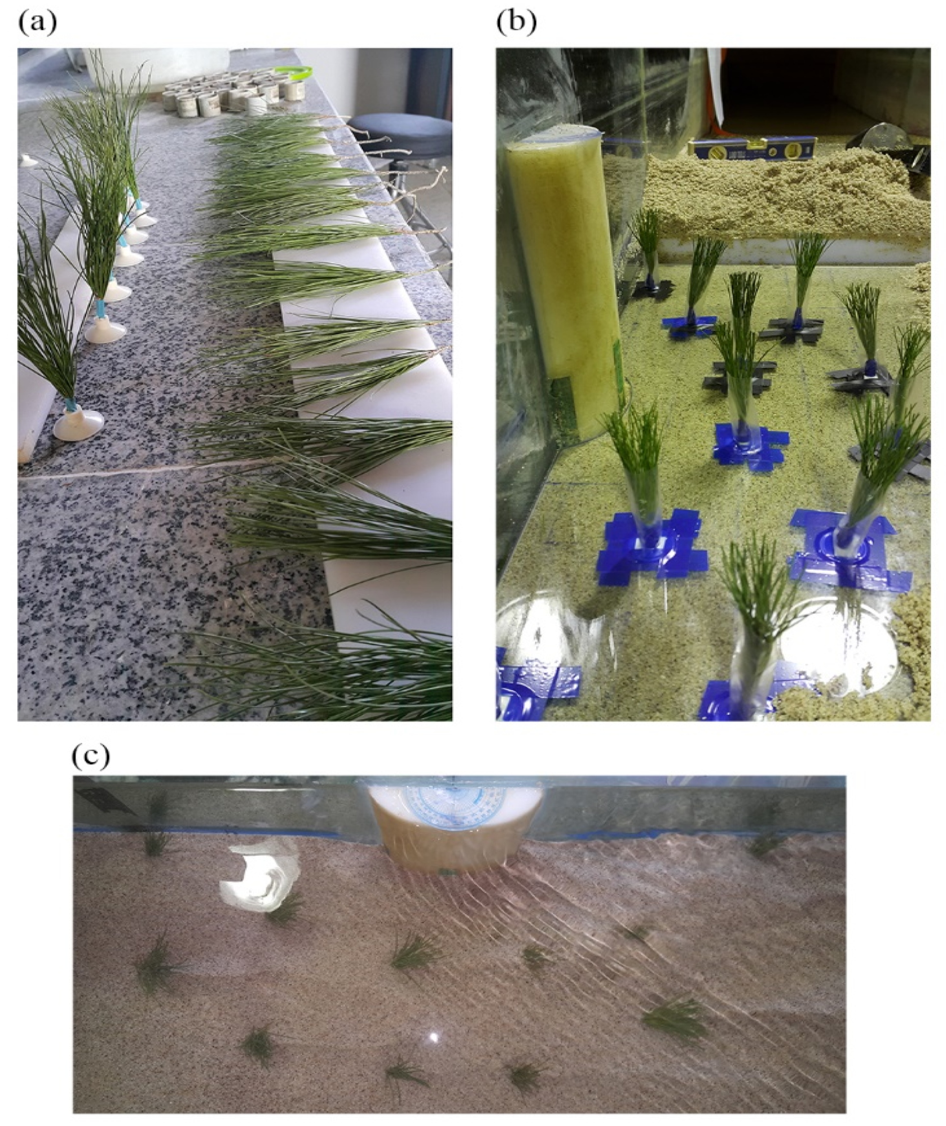
Abstract
:1. Introduction
2. Materials and Methods
3. Results and Discussions
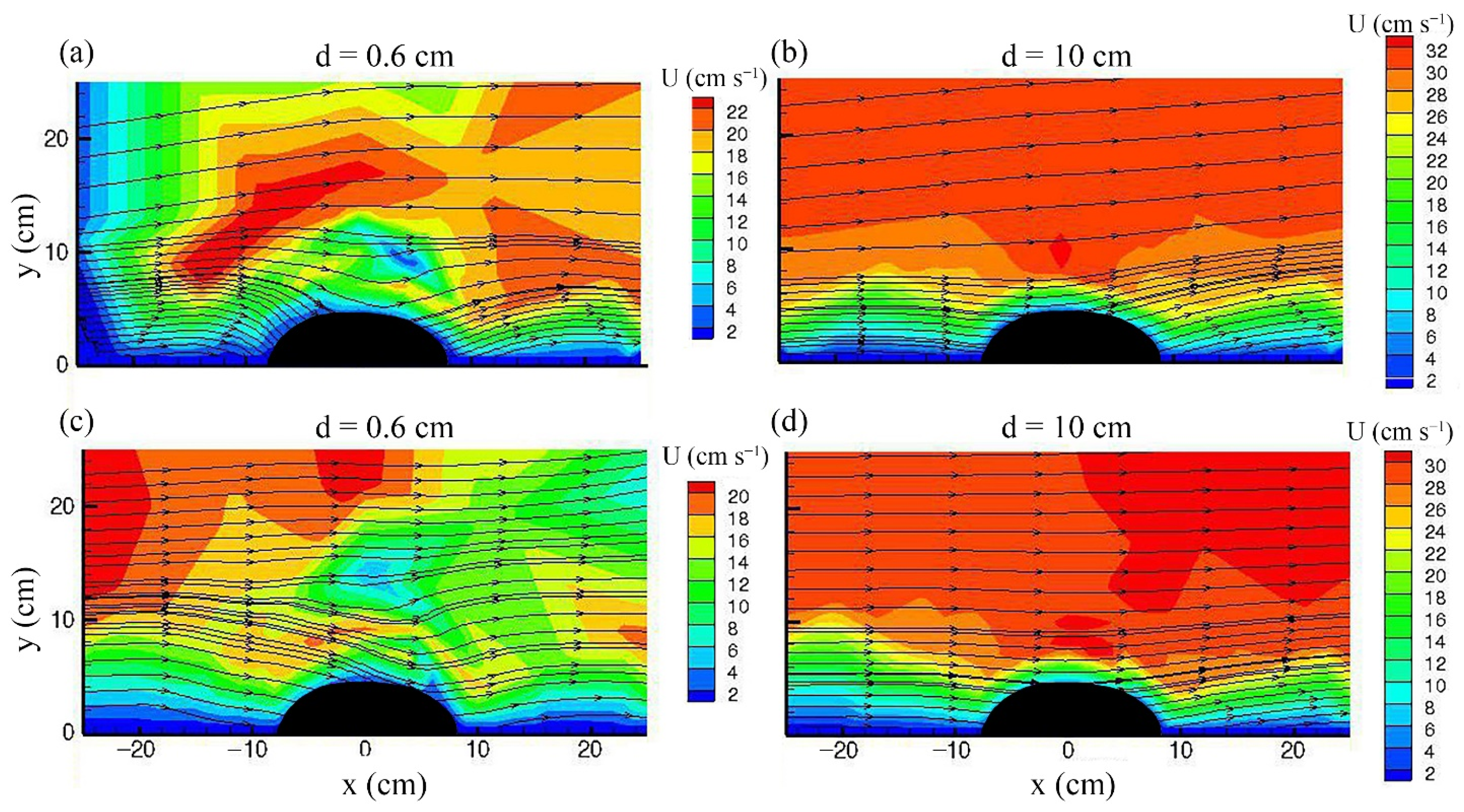
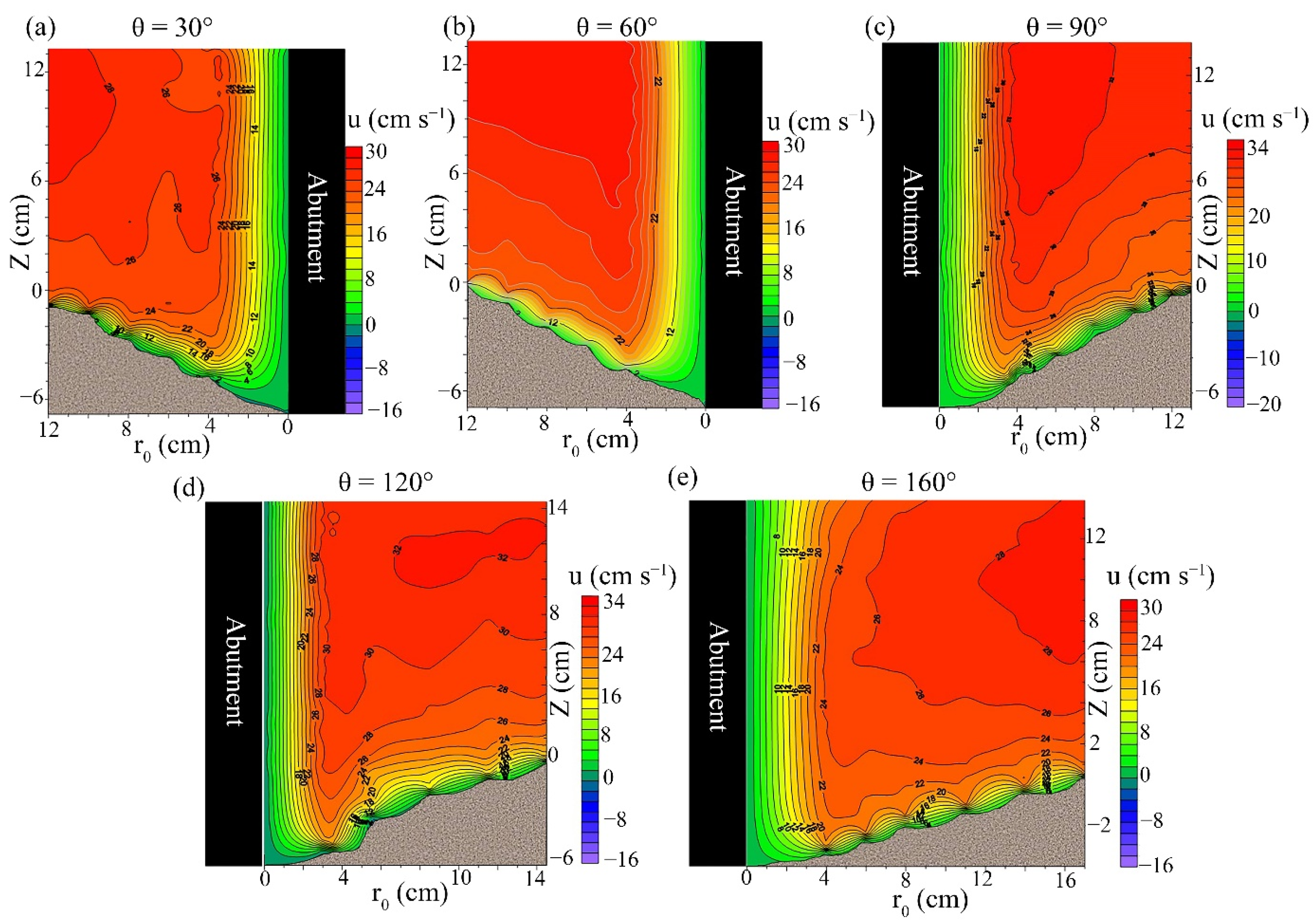
3.1. Velocity Field around the Abutment
- (1)
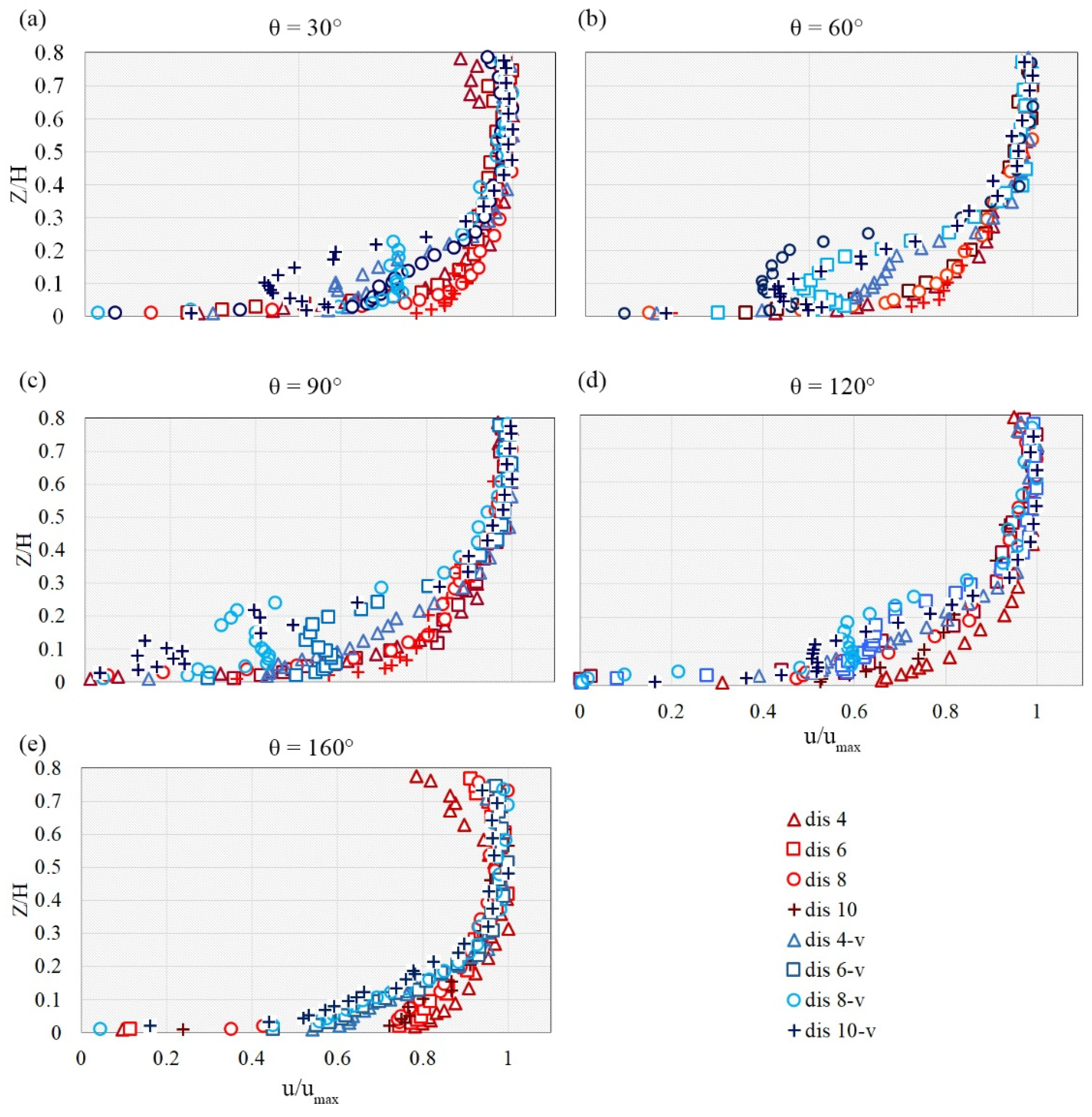
- The larger the distance from the abutment in the radial direction, the more the skewness in the distribution pattern of tangential velocity, especially at the upstream face of the abutment in an un-vegetated channel. Additionally, with the increase in the azimuthal angle (moving downstream), the skewness decreased. In other words, by moving downstream, the tangential velocity near the scoured bed tended to increase.
- (2)
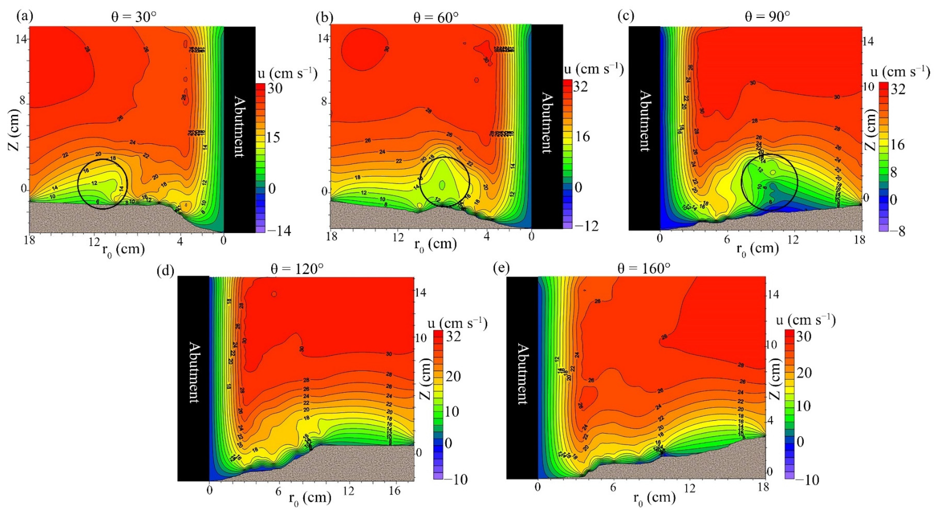
- For the vegetated bed case, the tangential velocity profile distribution had an “S” shape (changed near the scour bed), and this can be seen at all azimuthal angles, except the 160°.
- (3)
- (4)
- For the case with a vegetated bed, the velocity gradient near the channel bed became negative with the increase in the radial distance from the abutment, especially between 5 cm and 12 cm at all azimuthal angles, except the 160°. With the increase in the azimuth angle, the tangential velocity increased slower than the case without vegetation in bed (Mostly at z < 0.3h).
3.2. Reynolds Shear Stress Distribution
3.3. Turbulence Intensity
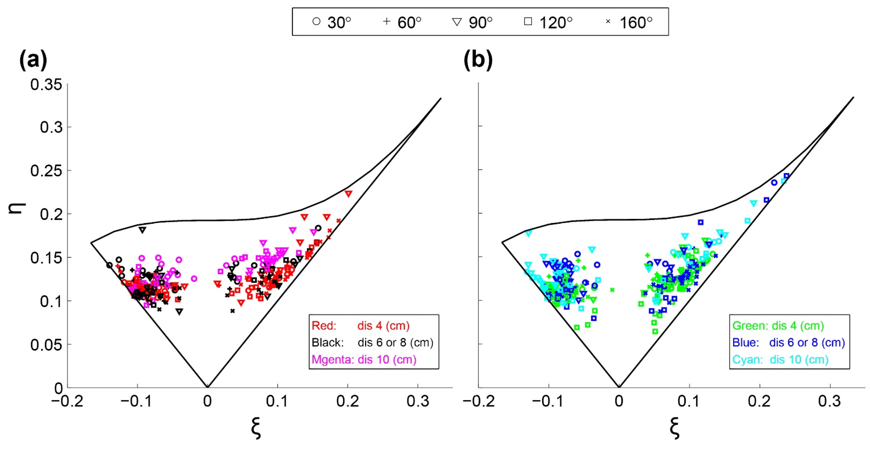
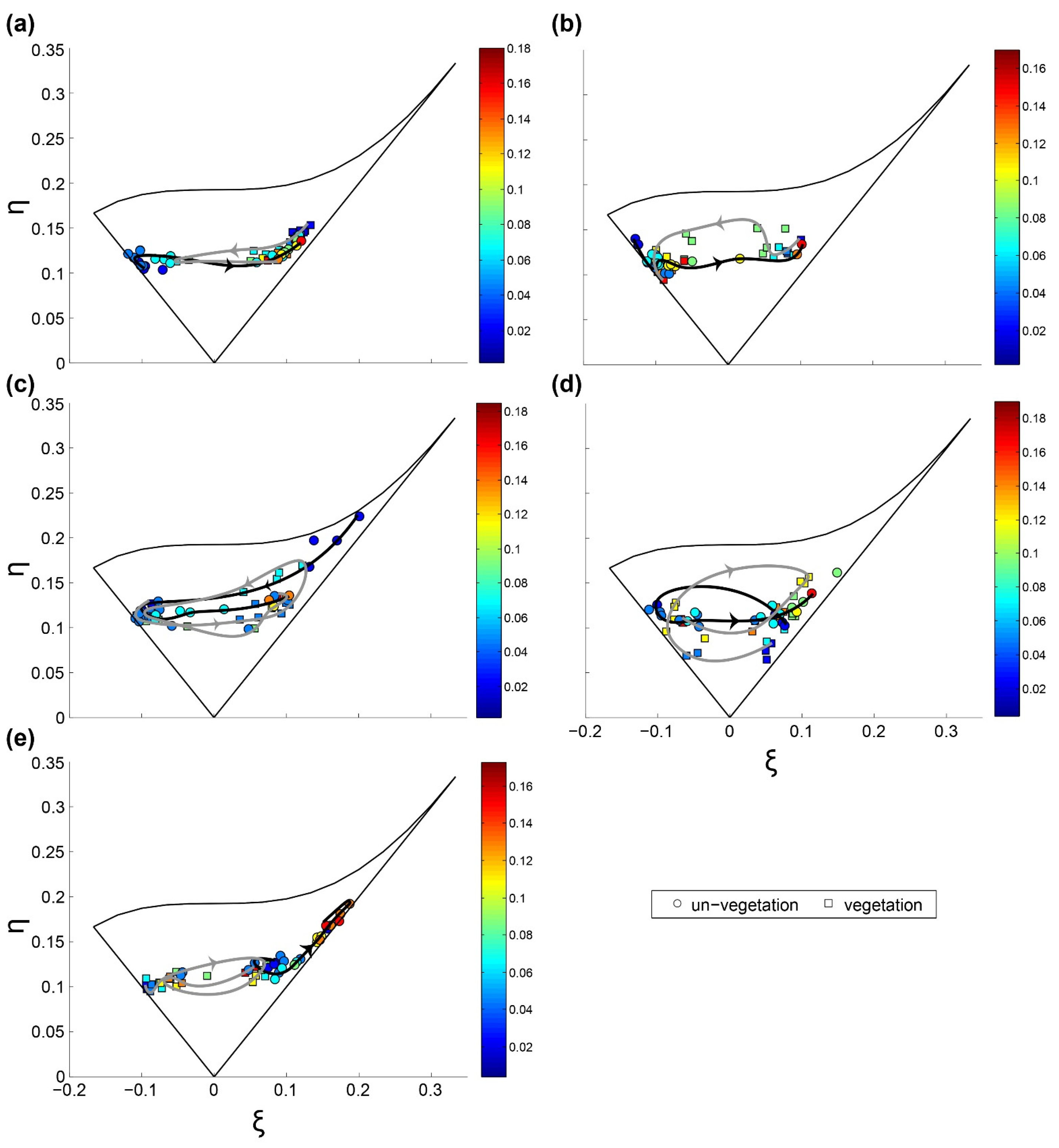
3.4. Reynolds Stress Anisotropy
4. Conclusions
- (1)
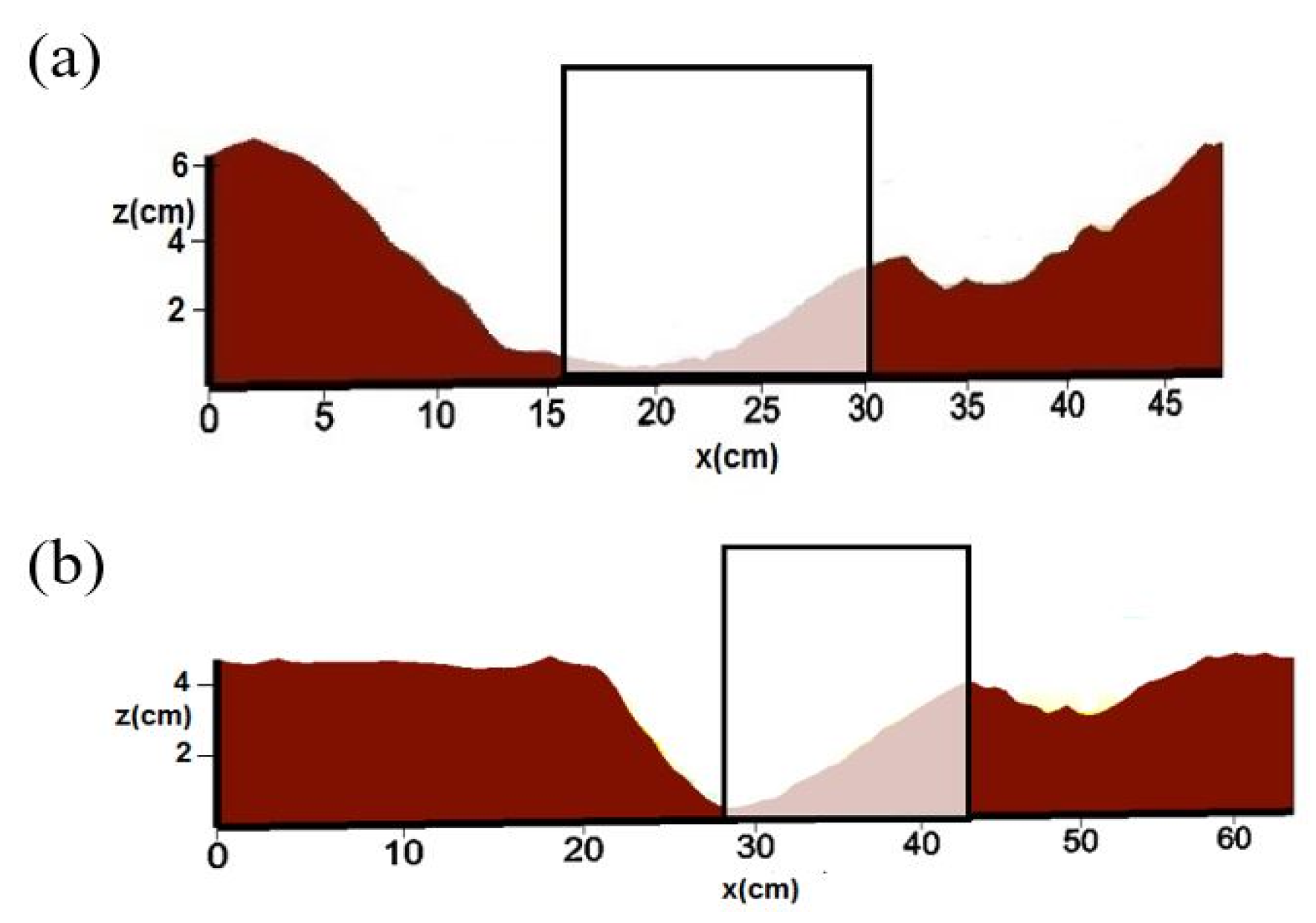
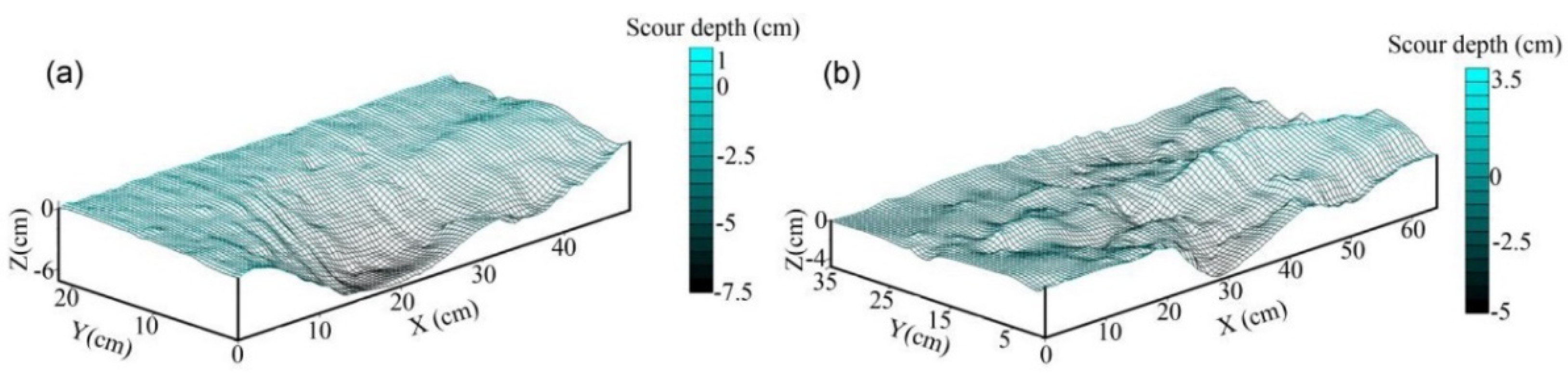
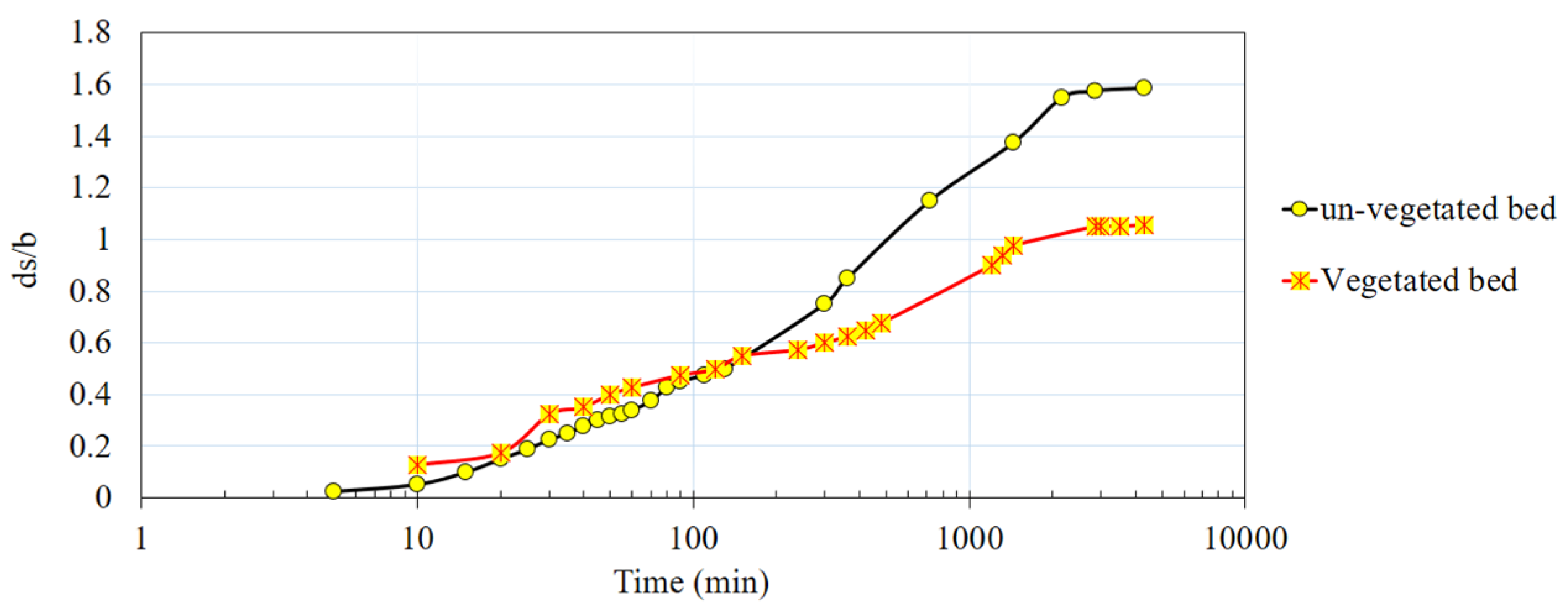
- Compared to the case of an un-vegetated bed, with vegetation around the abutment, the maximum scour depth occurred at the abutment tip instead of the upstream nose of the abutment. The presence of vegetation in the channel decreases the maximum values of the 3D velocity components (except for the positive values of w downstream and near the scour bed) and reduces the turbulence intensities inside the scour hole. For this experimental study, the presence of vegetation in the channel bed caused a reduction of 34.8% of the scour depth. The time required for achieving the equilibrium condition also decreased. Interestingly, within the first 120 min of the experiments, the scour depth for the case with vegetation in the bed was slightly higher than that for the case without vegetation.
- (2)
- The circulation and vortices have been weakened due to the presence of vegetation in the channel bed. In other words, the primary vortex for the case of an un-vegetated bed was stronger than that for the vegetated bed. The turbulence kinetic energy inside the scour hole is reduced.
- (3)
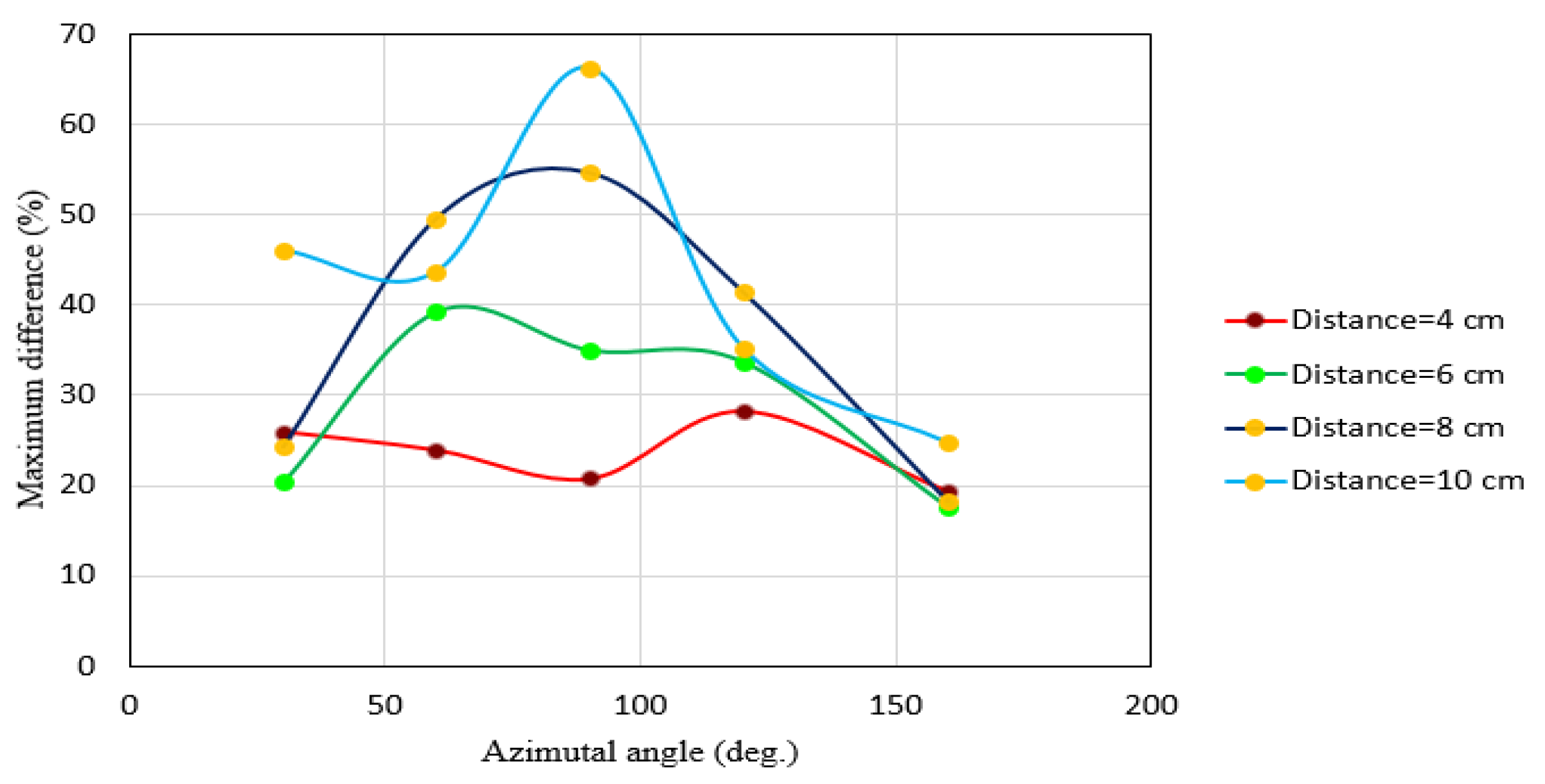
- The tangential velocity component was always positive and decreased rapidly near the scour bed, especially around the upstream face of the abutment. Additionally, the deceleration process of flow has proceeded slowly with vegetation in the channel bed. The tangential velocity increased with the increase in the azimuthal angle for both vegetated and un-vegetated cases, but the rate of deceleration at θ = 90° for the vegetated case was greater than those of θ = 30°, 60°. The maximum tangential velocity difference between two cases was observed at an angle of 90°. With vegetation’s presence, the tangential velocity profile (at all angles except the 160°) near the bed had changed to an “S” shape, which showed two turning points. Near the vegetated bed, the tangential velocity gradient with radial distance from the abutment became negative, especially between 5 cm to 12 cm (except at 160°).
- (4)
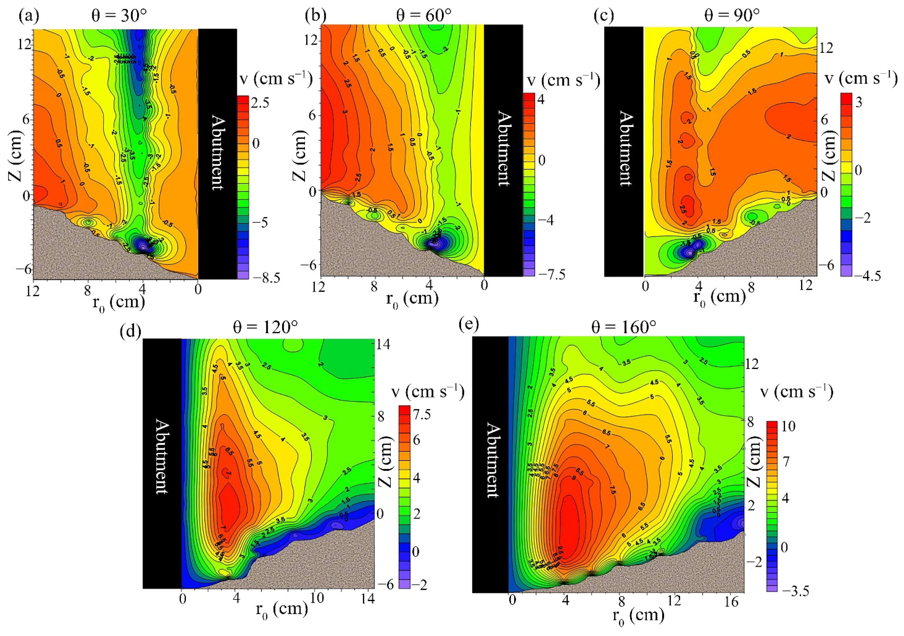
- The contours of radial velocity (v) upstream of the abutment (30° to 90°) had negative values for the case with vegetation in the bed within the scour hole (z ≤ 0) and above it (z ≥ 0), different from that for the case of un-vegetated bed. Downstream of the abutment, the sign change in radial velocity was observed for the case of the un-vegetated bed only at 90° and for the case of the vegetated bed at θ = 90°, 120°. This indicated a week flow reversal as a result of backflow. For the vegetated bed, variation in radial velocity inside the scour hole was less than that for the un-vegetated one (except 90° near the scour bed), indicating reduction in the primary vortex by vegetation.
- (5)
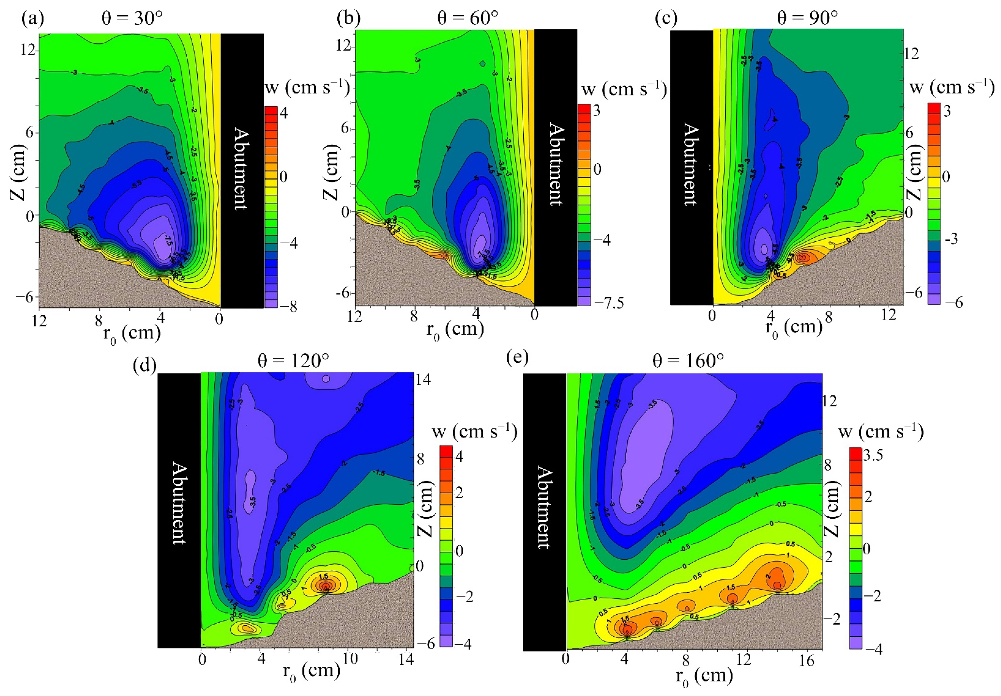
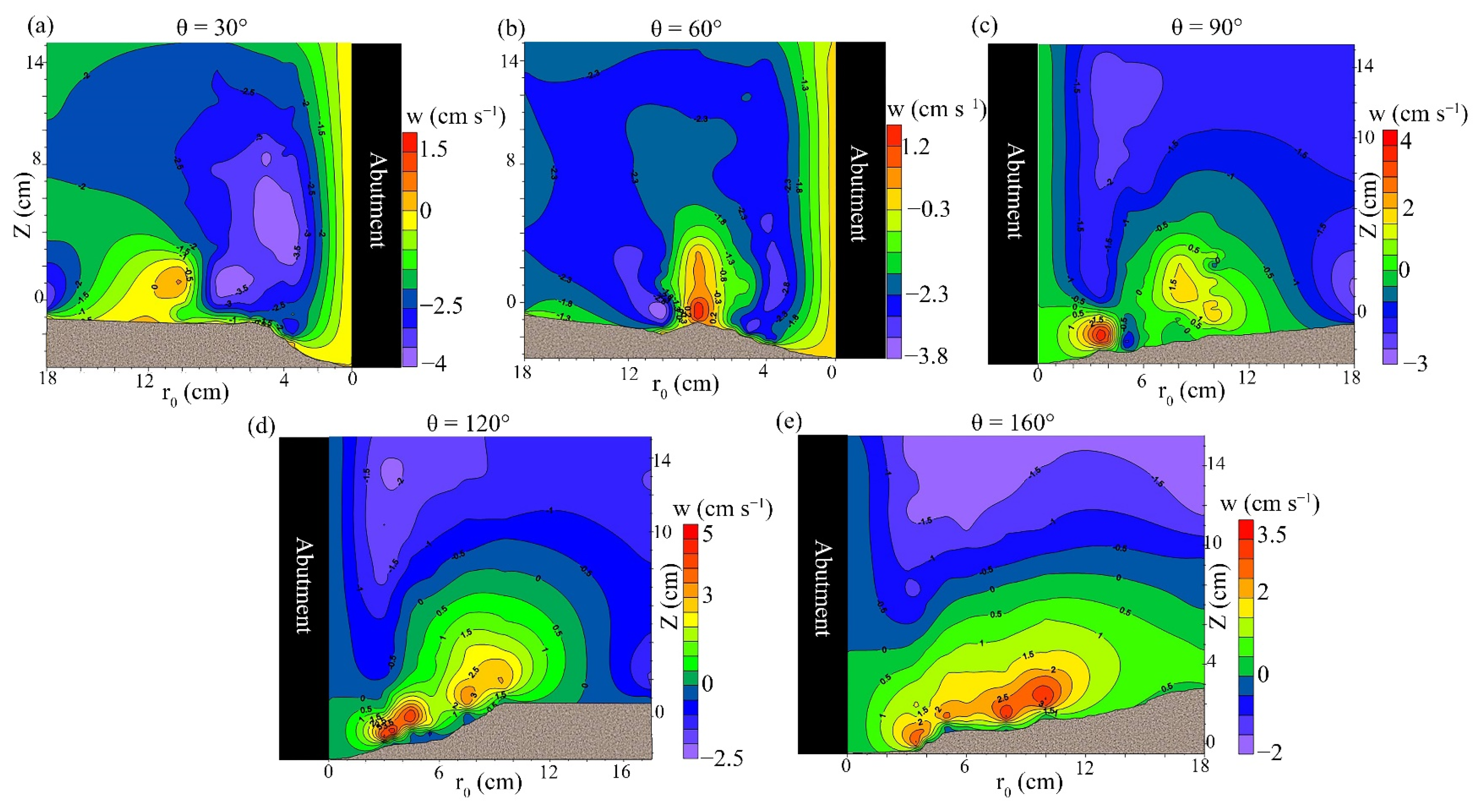
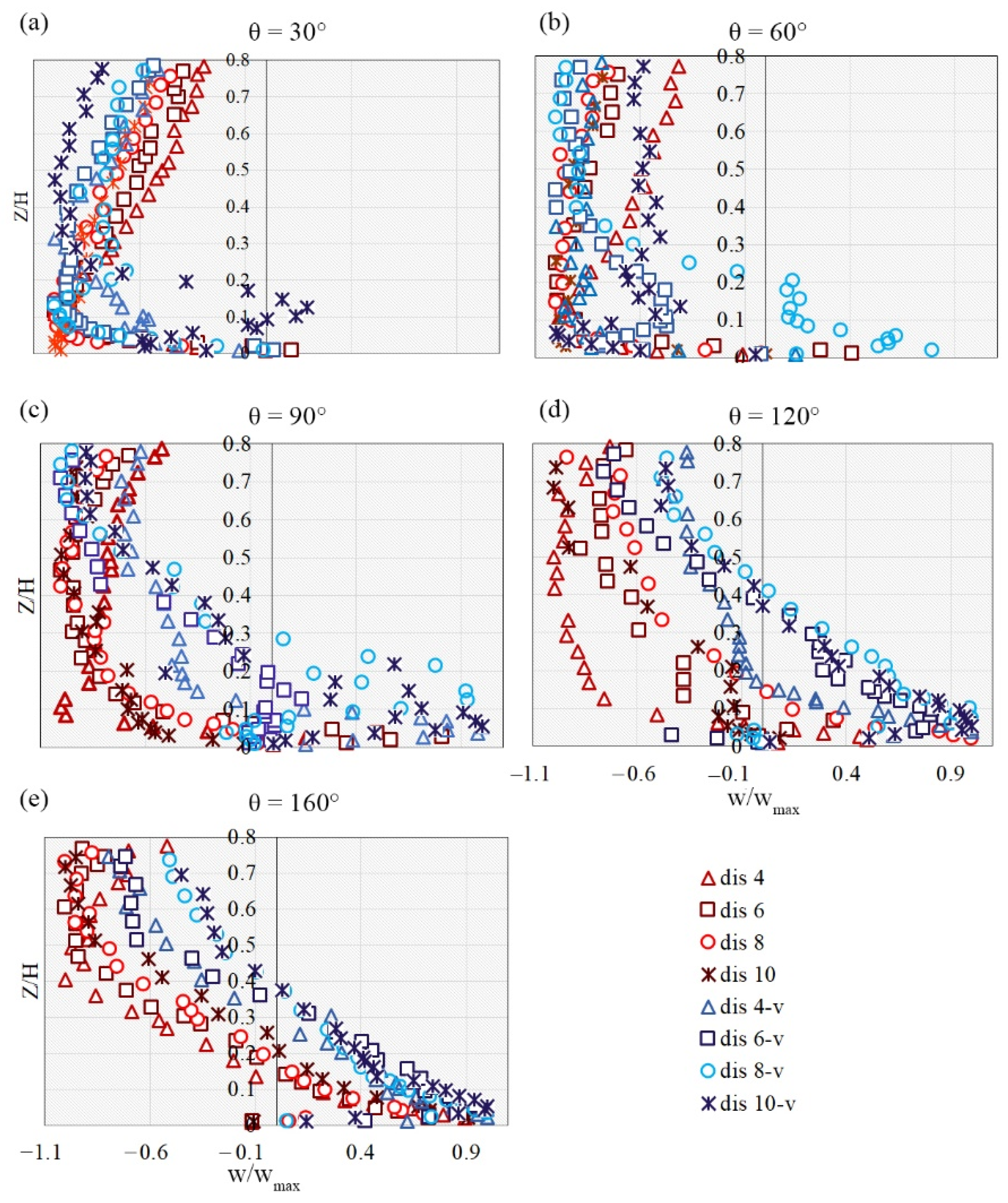
- For both vegetated and un-vegetated cases, the magnitude of the vertical velocity (w) toward the scour bed increased significantly, resulting in the powerful downflow around the abutment. For the case with vegetation in the bed inside the scour hole upstream of the abutment, the magnitude of the negative vertical velocity is diminished in this region compared to that for the un-vegetated bed, indicating that the power of downflow leads to a reduction of the primary vortices. The extent of the positive vertical velocities for the case with vegetation in the bed was increased and covered broader if the azimuthal angle was more than 90°, compared to the un-vegetated case. The maximum positive vertical velocities were observed at 160° for the un-vegetated bed and 120° for vegetation. It is found that vegetation could not significantly reduce the effect of upward flow in the downstream region adjacent to the abutment due to the suction that takes place.
- (6)
- Although radial and vertical velocities played an utmost important role in the flow field, the effect of tangential velocity was the highest, implying that the tangential velocity (u) contributed more to the turbulence intensities, Reynolds shear stress, and consequently the development of the scour holes.
- (7)
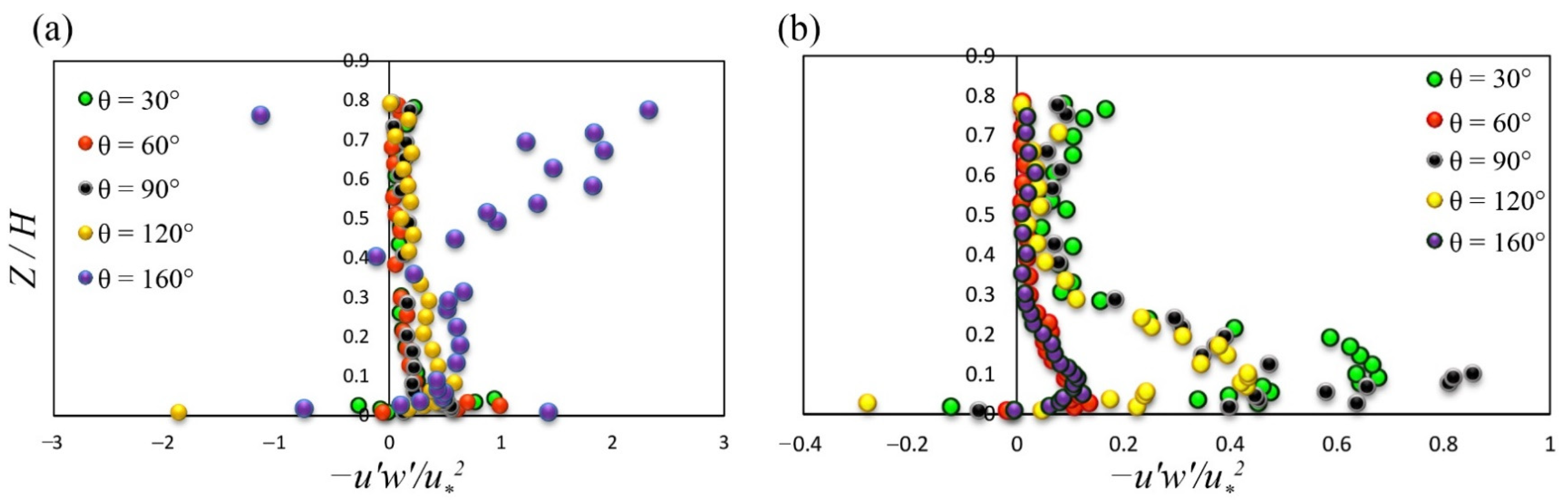
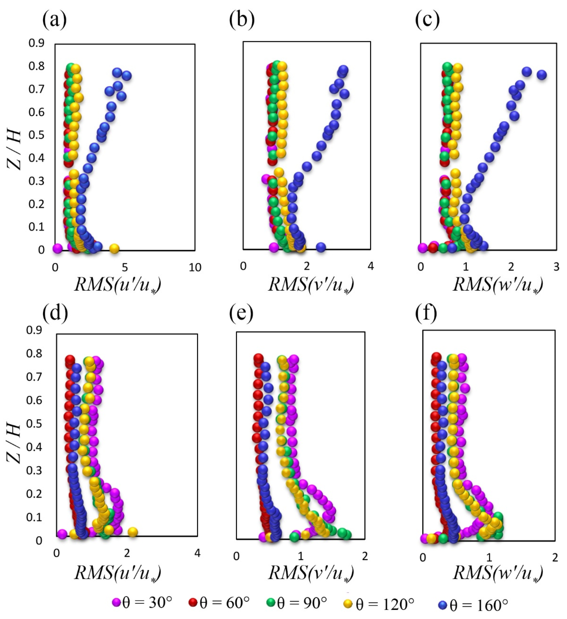
- The presence of vegetation in the bed dramatically reduces the Reynolds shear stress component, except at the distance of 4 cm and 160° near the scour bed. For the case of the un-vegetated bed, the convex distribution of Reynolds shear stress (−u’w’) was observed at all angles from 0° to 120°, except at a distance of 10 cm. With vegetation, Reynolds shear stress profiles were convex at all azimuthal angles and had a certain trend. The magnitude of negative Reynolds shear stress (−u’w’) confirms the development of wake zones downstream of the abutment, which occur at 120° for the vegetated bed and 160° for the case of the un-vegetated bed. These wake zones lead to the generation of strong turbulence. At a constant distance of 4 cm from the abutment, inside the scour hole, the vertical distribution of Reynolds shear stress and turbulence intensity possessed a convex shape. Near the scour bed, with the increase in the azimuthal angle (except 90°), both Reynolds shear stress and turbulence intensity decreased for the case of the vegetated bed. For the case of an un-vegetated bed, the maximum stress occurred near the bed at an angle of θ = 160°.
- (8)
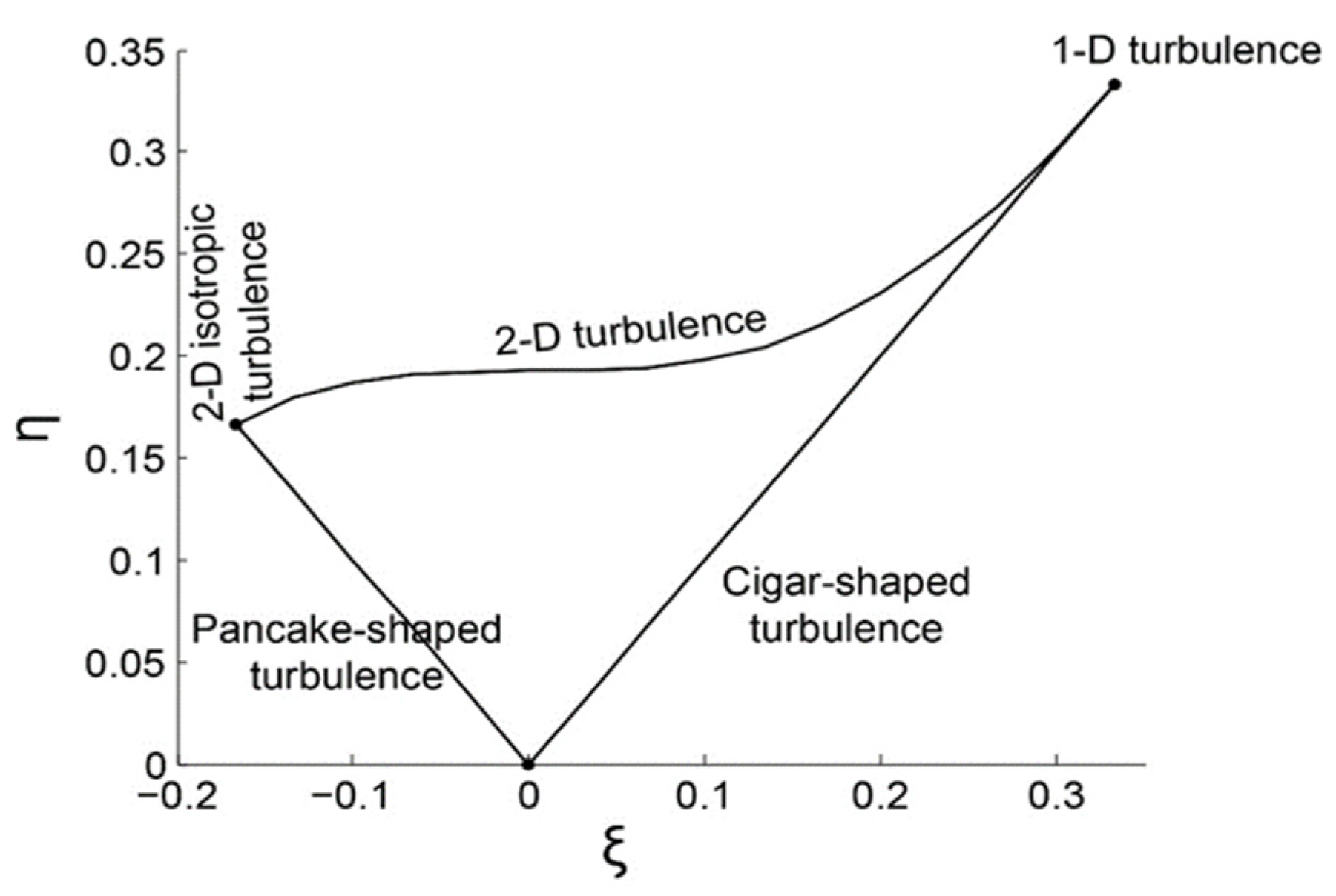
- By placing vegetation in the bed, for the vegetated bed, the flow tends to be more isotropic than that for the un-vegetated case. For the un-vegetated bed, the anisotropy level increases with the radial distance from the abutment due to the turbulence triangle. Moreover, at the upstream face of the abutment, most of the data points in the Lumley triangle tend to be pancake-shaped turbulence. However, for the case of a vegetated bed, there was a tendency to be cigar-shaped. Downstream of the abutment, due to flow separation, there was no definite trend. For the un-vegetated bed, upstream of the abutment, the anisotropy at a close distance of 4 cm from the abutment changes from pancake-shaped to cigar-shaped with the increase in the vertical distance (from the scour bed). For the case of a vegetated bed, the anisotropy starts from the cigar shape then changes to the opposite direction. Inside the scour hole in this zone, the degree of anisotropy for the case of the vegetated bed is larger than that for the un-vegetated bed. Downstream of the abutment, for the case of the un-vegetated bed, the anisotropy of turbulence is more uniform at θ = 160° and presents a tendency toward the cigar-shaped boundary. The highest degree of anisotropy for the case of an un-vegetated bed occurs near the scour hole or near the water surface. The vegetated bed was observed near the scour bed at θ = 30°, but it was located outside of the scour hole by increasing the angle.
- (9)
- For the case of an un-vegetated bed, inside the hole upstream of the abutment, the invariant function (F) value was greater than that for the vegetated bed. Downstream of the abutment, however, it was the opposite. Moreover, the F value for the case of the un-vegetated bed near the scour hole at θ = 90° corresponds to two-dimensional isotropy. For the vegetated bed, however, inside the hole at θ = 120°, F leads to three-dimensional isotropy, with the highest amount of all the azimuthal angles for both cases.
Author Contributions
Funding
Institutional Review Board Statement
Informed Consent Statement
Data Availability Statement
Conflicts of Interest
References
- Sui, J.; Fang, D.; Karney, B.W. An experimental study into local scour in a channel caused by a 90 bend. Can. J. Civ. Eng. 2006, 33, 902–911. [Google Scholar] [CrossRef]
- Sui, J.; Faruque, M.; Balachandar, R. Influence of channel width and tailwater depth on local scour caused by square jets. J. Hydro-Environ. Res. 2008, 2, 39–45. [Google Scholar] [CrossRef]
- Afzalimehr, H.; Moradian, M.; Singh, V.P. Flow field around semi-elliptical abutments. J. Hydrol. Eng. 2018, 23, 04017057. [Google Scholar] [CrossRef]
- Sui, J.; Faruque, M.; Balachandar, R. Local scour caused by submerged square jets under model ice cover. J. Hydraul. Eng. 2009, 135, 316–319. [Google Scholar] [CrossRef]
- Wu, P.; Hirshfield, F.; Sui, J. Armour layer analysis of local scour around bridge abutments under ice cover. River Res. Appl. 2015, 31, 736–746. [Google Scholar] [CrossRef]
- Arneson, L.; Zevenbergen, L.; Lagasse, P.; Clopper, P. Evaluating Scour at Bridges–Federal Highway Administration Hydraulic Engineering Circular No. 18, 5th ed.; FHWA-HIF-12-003; FHWA: Washington, DC, USA, 2012.
- Richardson, J.; Richardson, E. The fallacy of local abutment scour equations. In Proceedings of the Hydraulic Engineering, San Francisco, CA, USA, 25–30 July 1993; pp. 749–754. [Google Scholar]
- Melville, B.W. Pier and abutment scour: Integrated approach. J. Hydraul. Eng. 1997, 123, 125–136. [Google Scholar] [CrossRef]
- Kothyari, U.; Ranga Raju, K. Scour around spur dikes and bridge abutments. J. Hydraul. Res. 2001, 39, 367–374. [Google Scholar] [CrossRef]
- Dey, S. Fluvial Hydrodynamics; Springer: Berlin/Heidelberg, Germany, 2014. [Google Scholar]
- Kw An, R.T.; Melville, B.W. Local scour and flow measurements at bridge abutments. J. Hydraul. Res. 1994, 32, 661–673. [Google Scholar] [CrossRef]
- Melville, B.W.; Coleman, S.E. Bridge Scour; Water Resources Publication: Littleton, CO, USA, 2000. [Google Scholar]
- Wu, P.; Hirshfield, F.; Sui, J.; Wang, J.; Chen, P.-P. Impacts of ice cover on local scour around semi-circular bridge abutment. J. Hydrodyn. 2014, 26, 10–18. [Google Scholar] [CrossRef]
- Wu, P.; Balachandar, R.; Sui, J. Local scour around bridge piers under ice-covered conditions. J. Hydraul. Eng. 2016, 142, 04015038. [Google Scholar] [CrossRef]
- Sui, J.; Afzalimehr, H.; Samani, A.K.; Maherani, M. Clear-water scour around semi-elliptical abutments with armored beds. Int. J. Sediment Res. 2010, 25, 233–245. [Google Scholar] [CrossRef]
- Yang, Y.; Xiong, X.; Melville, B.W.; Sturm, T.W. Dynamic morphology in a bridge-contracted compound channel during extreme floods: Effects of abutments, bed-forms and scour countermeasures. J. Hydrol. 2021, 594, 125930. [Google Scholar] [CrossRef]
- Bressan, F.; Ballio, F.; Armenio, V. Turbulence around a scoured bridge abutment. J. Turbul. 2011, N3. [Google Scholar] [CrossRef]
- Koken, M. Coherent structures at different contraction ratios caused by two spill-through abutments. J. Hydraul. Res. 2018, 56, 324–332. [Google Scholar] [CrossRef]
- Namaee, M.R.; Sui, J. Velocity profiles and turbulence intensities around side-by-side bridge piers under ice-covered flow condition. J. Hydrol. Hydromech. 2020, 68, 70–82. [Google Scholar] [CrossRef] [Green Version]
- Lumley, J.L.; Newman, G.R. The return to isotropy of homogeneous turbulence. J. Fluid Mech. 1977, 82, 161–178. [Google Scholar] [CrossRef] [Green Version]
- Sarkar, S.; Dey, S. Turbulent length scales and anisotropy downstream of a wall mounted sphere. J. Hydraul. Res. 2015, 53, 649–658. [Google Scholar] [CrossRef]
- Sharma, A.; Kumar, B. Anisotropy Properties of Turbulence in Flow Over Seepage Bed. J. Fluids Eng. 2021, 144, 021501. [Google Scholar] [CrossRef]
- Ali, N.; Hamilton, N.; Calaf, M.; Cal, R.B. Classification of the Reynolds stress anisotropy tensor in very large thermally stratified wind farms using colormap image segmentation. J. Renew. Sustain. Energy 2019, 11, 063305. [Google Scholar] [CrossRef]
- Mera, I.; Franca, M.J.; Anta, J.; Peña, E. Turbulence anisotropy in a compound meandering channel with different submergence conditions. Adv. Water Resour. 2015, 81, 142–151. [Google Scholar] [CrossRef]
- Velasco, D.; Bateman, A.; Redondo, J.M.; DeMedina, V. An open channel flow experimental and theoretical study of resistance and turbulent characterization over flexible vegetated linings. Flow Turbul. Combust. 2003, 70, 69–88. [Google Scholar] [CrossRef]
- Piedelobo, L.; Taramelli, A.; Schiavon, E.; Valentini, E.; Molina, J.-L.; Nguyen Xuan, A.; González-Aguilera, D. Assessment of green infrastructure in Riparian zones using copernicus programme. Remote Sens. 2019, 11, 2967. [Google Scholar] [CrossRef] [Green Version]
- Luhar, M.; Rominger, J.; Nepf, H. Interaction between flow, transport and vegetation spatial structure. Environ. Fluid Mech. 2008, 8, 423–439. [Google Scholar] [CrossRef]
- Nepf, H.M. Hydrodynamics of vegetated channels. J. Hydraul. Res. 2012, 50, 262–279. [Google Scholar] [CrossRef] [Green Version]
- Kabiri, F.; Afzalimehr, H.; Sui, J. Flow structure over a wavy bed with vegetation cover. Int. J. Sediment Res. 2017, 32, 186–194. [Google Scholar] [CrossRef]
- D’Ippolito, A.; Calomino, F.; Alfonsi, G.; Lauria, A. Drag coefficient of in-line emergent vegetation in open channel flow. Int. J. River Basin Manag. 2021, 1–11. [Google Scholar] [CrossRef]
- Afzalimehr, H.; Moghbel, R.; Gallichand, J.; Sui, J. Investigation of turbulence characteristics in channel with dense vegetation. Int. J. Sediment Res. 2011, 26, 269–282. [Google Scholar] [CrossRef]
- Keshavarz, A.; Afzalimehr, H.; Singh, V.P. Impact of unfavourable pressure gradient and vegetation bed on flow. J. Hydraul. Eng. 2015, 4, 10–16. [Google Scholar]
- Afzalimehr, H.; Bakhshi, S.; Gallichand, J.; Sui, J. Effect of vegetated-banks on local scour around a wing-wall abutment with circular edges. J. Hydrodyn. 2014, 26, 447–457. [Google Scholar] [CrossRef]
- Chiew, Y.-M.; Melville, B.W. Local scour around bridge piers. J. Hydraul. Res. 1987, 25, 15–26. [Google Scholar] [CrossRef]
- Dey, S.; Bose, S.K.; Sastry, G.L. Clear water scour at circular piers: A model. J. Hydraul. Eng. 1995, 121, 869–876. [Google Scholar] [CrossRef]
- Afzalimehr, H.; Moradian, M.; Gallichand, J.; Sui, J. Effect of adverse pressure gradient and different vegetated banks on flow. River Res. Appl. 2016, 32, 1059–1070. [Google Scholar] [CrossRef]
- Bolhassani, R.; Afzalimehr, H.; Dey, S. Effects of relative submergence and bed slope on sediment incipient motion under decelerating flows. J. Hydrol. Hydromech. 2015, 63, 295–302. [Google Scholar] [CrossRef] [Green Version]
- Bhandari, L.; Upadhyay, C.; Mohite, P.; Gupta, A.; Sarkar, S.; Panwar, V.S. Tensile test on pine needles and crack analysis of pine needles short fiber reinforced composites. IOSR J. Mech. Civ. Eng. (IOSRJMCE) E-ISSN 2015, 12, 2278-1684. [Google Scholar]
- Melville, B.W.; Chiew, Y.-M. Time scale for local scour at bridge piers. J. Hydraul. Eng. 1999, 125, 59–65. [Google Scholar] [CrossRef]
- Goring, D.G.; Nikora, V.I. Despiking acoustic Doppler velocimeter data. J. Hydraul. Eng. 2002, 128, 117–126. [Google Scholar] [CrossRef] [Green Version]
- Wahl, T. Analyzing ADV data using WinADV. In Proceedings of the Joint Conference on Water Resources Engineering and Water Resources Planning and Management, Minneapolis, MN, USA, 30 July–2 August 2000; pp. 1–10. [Google Scholar]
- Lança, R.M.; Fael, C.S.; Maia, R.J.; Pêgo, J.P.; Cardoso, A.H. Clear-water scour at comparatively large cylindrical piers. J. Hydraul. Eng. 2013, 139, 1117–1125. [Google Scholar] [CrossRef] [Green Version]
- Lee, S.O.; Sturm, T.W. Effect of sediment size scaling on physical modeling of bridge pier scour. J. Hydraul. Eng. 2009, 135, 793–802. [Google Scholar] [CrossRef]
- Shahmohammadi, R.; Afzalimehr, H.; Sui, J. Impacts of turbulent flow over a channel bed with a vegetation patch on the incipient motion of sediment. Can. J. Civ. Eng. 2018, 45, 803–816. [Google Scholar] [CrossRef]
- Shahmohammadi, R.; Afzalimehr, H.; Sui, J. Assessment of Critical Shear Stress and Threshold Velocity in Shallow Flow with Sand Particles. Water 2021, 13, 994. [Google Scholar] [CrossRef]
- Yamasaki, T.N.; Jiang, B.; Janzen, J.G.; Nepf, H.M. Feedback between vegetation, flow, and deposition: A study of artificial vegetation patch development. J. Hydrol. 2021, 598, 126232. [Google Scholar] [CrossRef]
- Jafari, R.; Sui, J. Velocity Field and Turbulence Structure around Spur Dikes with Different Angles of Orientation under Ice Covered Flow Conditions. Water 2021, 13, 1844. [Google Scholar] [CrossRef]
- Huai, W.-x.; Zhang, J.; Katul, G.G.; Cheng, Y.-g.; Tang, X.; Wang, W.-j. The structure of turbulent flow through submerged flexible vegetation. J. Hydrodyn. 2019, 31, 274–292. [Google Scholar] [CrossRef]
- Dey, S.; Barbhuiya, A.K. 3D flow field in a scour hole at a wing-wall abutment. J. Hydraul. Res. 2006, 44, 33–50. [Google Scholar] [CrossRef]
- Dey, S.; Barbhuiya, A.K. Turbulent flow field in a scour hole at a semicircular abutment. Can. J. Civ. Eng. 2005, 32, 213–232. [Google Scholar] [CrossRef]
- Siniscalchi, F.; Nikora, V.I.; Aberle, J. Plant patch hydrodynamics in streams: Mean flow, turbulence, and drag forces. Water Resour. Res. 2012, 48. [Google Scholar] [CrossRef] [Green Version]
- Pope, S.B. Turbulent Flows; Cambridge University Press: Cambridge, UK, 2000; Available online: https://www.cambridge.org/ir/academic/subjects/physics/nonlinear-science-and-fluid-dynamics/turbulent-flows?format=PB&isbn=9780521598866 (accessed on 20 October 2021).
- Lumley, J.L. Computational modeling of turbulent flows. In Advances in Applied Mechanics; Elsevier: Amsterdam, The Netherlands, 1979; Volume 18, pp. 123–176. [Google Scholar]


Publisher’s Note: MDPI stays neutral with regard to jurisdictional claims in published maps and institutional affiliations. |
© 2021 by the authors. Licensee MDPI, Basel, Switzerland. This article is an open access article distributed under the terms and conditions of the Creative Commons Attribution (CC BY) license (https://creativecommons.org/licenses/by/4.0/).
Share and Cite
Nabaei, S.F.; Afzalimehr, H.; Sui, J.; Kumar, B.; Nabaei, S.H. Investigation of the Effect of Vegetation on Flow Structures and Turbulence Anisotropy around Semi-Elliptical Abutment. Water 2021, 13, 3108. https://doi.org/10.3390/w13213108
Nabaei SF, Afzalimehr H, Sui J, Kumar B, Nabaei SH. Investigation of the Effect of Vegetation on Flow Structures and Turbulence Anisotropy around Semi-Elliptical Abutment. Water. 2021; 13(21):3108. https://doi.org/10.3390/w13213108
Chicago/Turabian StyleNabaei, Seyedeh Fatemeh, Hossein Afzalimehr, Jueyi Sui, Bimlesh Kumar, and Seyed Hamidreza Nabaei. 2021. "Investigation of the Effect of Vegetation on Flow Structures and Turbulence Anisotropy around Semi-Elliptical Abutment" Water 13, no. 21: 3108. https://doi.org/10.3390/w13213108