Catchment Scale Evaluation of Multiple Global Hydrological Models from ISIMIP2a over North America

Abstract

A satisfactory performance of hydrological models under historical climate conditions is considered a prerequisite step in any hydrological climate change impact study. Despite the significant interest in global hydrological modeling, few systematic evaluations of global hydrological models (gHMs) at the catchment scale have been carried out. This study investigates the performance of 4 gHMs driven by 4 global observation-based meteorological inputs at simulating weekly discharges over 198 large-sized North American catchments for the 1971–2010 period. The 16 discharge simulations serve as the basis for evaluating gHM accuracy at the catchment scale within the second phase of the Inter-Sectoral Impact Model Intercomparison Project (ISIMIP2a). The simulated discharges by the four gHMs are compared against observed and simulated weekly discharge values by two regional hydrological models (rHMs) driven by a global meteorological dataset for the same period. We discuss the implications of both modeling approaches as well as the influence of catchment characteristics and global meteorological forcing in terms of model performance through statistical criteria and visual hydrograph comparison for catchment-scale hydrological studies. Overall, the gHM discharge statistics exhibit poor agreement with observations at the catchment scale and manifest considerable bias and errors in seasonal flow simulations. We confirm that the gHM approach, as experimentally implemented through the ISIMIP2a, must be used with caution for regional studies. We find the rHM approach to be more trustworthy and recommend using it for hydrological studies, especially if findings are intended to support operational decision-making.

1. Introduction

Climate change impact research is currently moving onto the provision of climate projection services by impact models for use in developing adaptation strategies in various environmental sectors [1]. In the water sector, many worldwide initiatives have emerged from organizations and research centers, with the production and dissemination of information on projected climate change impacts on water resources through specific hydrological indicators. Such information is usually designed to cater to the needs of water and energy domain practitioners and is intended for use (and is sometimes used) in operational decision-making. Data suppliers and modelers thus have the responsibility of providing reliable and accurate information on the impacts of climate change on water as local adaptation measures stem from that. Projected climate change impacts on water resources are typically estimated by driving a hydrological model with climate projections from regional climate models or global climate models processed with statistical downscaling approaches to obtain hydrological projections at the catchment scale. Such work normally makes use of a hydrological model calibrated and validated at the catchment under study.

Global hydrological models (gHMs; spatial resolution approximately of 0.5 × 0.5) are often used to provide a general picture of hydrological features at the continental or global scale [2]. Only a limited number gHMs are calibrated for climatic regions or large-scale river basins, such as the WAter and Snow balance MODelling system (WASMOD; [3]) and Water Global Assessment and Prognosis (WaterGAP; [4]). The gHMs display contrasting model features regarding reservoir storage, the crop growth model, the energy balance model, and sub-grid variability.

The main output of all gHMs is the simulated runoff at the grid level, which is further aggregated to the catchment scale and routed to the outlet based on the number of grids within the catchment (see [5] for a gHM review). Although the gHMs represent a significant advancement in providing precious estimates of water resources, as compared to basic empirical statistical analyses, they were designed to be effective for global-scale hydrological studies [5]. Though they have been increasingly used in various studies [6], their implementation at the regional or catchment scale involves many uncertainties due to their coarse resolution and global parameterization [7]. It is challenging to affirm that the quality of the performance of gHMs will be satisfactory locally and will provide an accurate description of the hydrological processes for the catchment of interest [8,9]. Several studies have shown the quite poor or weak performance of gHMs in most cases, for large river basins as well as for relatively small catchments (e.g., [4,7,10,11,12,13]).

Regional hydrological models (rHMs), in contrast, are widely employed at the catchment scale for various purposes, such as the modeling of flow dynamics and its components [14,15]), understanding hydrological processes [16], streamflow forecasting [17,18,19], predicting discharges in ungauged catchments [20,21] and evaluating the likely impacts of climate change on hydro systems [22,23]. They have higher spatial resolutions and require more detailed inputs to simulate hydrological processes. Contrary to the gHMs, which are mostly not calibrated, the rHMs are calibrated to match the observed discharge values at the regional or catchment scale; hence, they are expected to represent the observed discharge dynamics more accurately than the gHMs [9,11]. However, few rHMs are implemented for multiple catchments or large regions [23,24], mainly because their implementation and calibration involve great numerical modeling effort.

rHMs are commonly calibrated and validated over a historical period to assess their performance, and this is a prerequisite for conducting a climate change impact study. With the rise in the number of impact studies involving gHMs [7,25,26], it is becoming increasingly important to explore their accuracy through an intercomparison between gHMs and rHMs at the catchment scale. In its second phase (phase 2a), the Inter-Sectoral Impact Model Intercomparison Project (ISIMIP; https://www.isimip.org/about/ accessed on 1 November 2021) provides simulated discharges from several gHMs globally from which simulations for individual large-scale river basins can be extracted. The gHMs in the ISMIP2a are driven by multiple observation-based meteorological datasets. A systematic assessment of the gHMs’ performance, along with the uncertainty associated with the choice of the driving meteorological inputs, is of great importance since it provides the basis for the following impact studies. Some studies consider multiple gHMs (e.g., [11,12,21,27,28]) with several forcing inputs (e.g., [6,29,30]), but with a macro (i.e., continental to global scale) or regional (e.g., [4,11,31,32,33]) scale evaluation of the simulated discharges by the gHMs. Among these works, only a few examine the gHMs’ performance for river basins in North America (NA; [11,12,34,35]). A study [10] evaluated several gHMs globally, driven by one forcing data for 966 small catchments (<5.000 km²), including the NA region. It found significant inter-gHM performance differences, with substantial biases in the driving forcing data compared to the observations. Another study [6] provided an intercomparison of multiple gHMs driven by four driving forcing data for two large dam-regulated river basins in NA. It showed profound discrepancies in the simulated river flows among the gHMs. The weak performance of the gHMs at reproducing the seasonal discharge cycle for NA and Pan-Artic (including Canadian/USA catchments) river basins has also been reported [11,12]. However, the use of small-sized catchments is a limitation regarding the spatial resolution of the gHMs (0.5-degree grid cells), while a weak sample of catchments precludes a spatially detailed assessment of the gHM’s performance.

Based on a multi-model approach composed of four gHMs (DBH, H08, LPJml, and PCR-GLOBWB) and two rHMs (GR4J and HMETS) driven by multiple forcing meteorological datasets over 198 large-sized NA catchments for the 1971–2010 period, this study aims at contributing to the ISIMIP2a topic for operational use purposes by: (1) assessing the gHMs’ performance in terms of simulating seasonal flow dynamics; (2) comparing the gHMs’ performance with that of the rHMs; and (3) based on (1) and (2), exploring the influence of the global driving datasets and catchment characteristics on gHM performance. The four gHMs are selected as they contain the varsoc socio-economic scenario for multiple forcing meteorological datasets over NA; the selected rHMs usually display reliable accuracy in data-deficient conditions due to their quite simple and parsimonious structure [36,37]. Overall, this work provides key information for subsequent impact studies, supporting decision-making based on the gHMs for the NA region covered by the global ISIMIP2 domain.

2. Materials and Methods

This section details the methodology of the multi-model approach (Figure 1) and the rationale behind the choices implemented in this study. The study area and selection of catchments are first described, followed by the extraction of gHM discharge values, as well as the application of hydrological simulations using the typical rHM approach. Finally, the statistical model performance criteria are described.

2.1. Study Area

The catchments are selected from the HYSETS large-scale database (https://osf.io/rpc3w/ accessed on 1 November 2021), which is comprised of 14,425 catchments in the NA region. The HYSETS database includes a wide array of hydrometeorological data over the 1950–2018 period: (1) daily precipitation, minimum and maximum temperature products from seven data sources; (2) hydrometric gauging station discharge time series from one data source per country (Canada, contiguous U.S., Mexico); (3) SNODAS and ERA5-Land snow water equivalent; and (5) catchment properties from PAVICS-Hydro (area, elevation slope, land use, soil properties, and other physiographic information). See [38] for additional information regarding the HYSETS database.

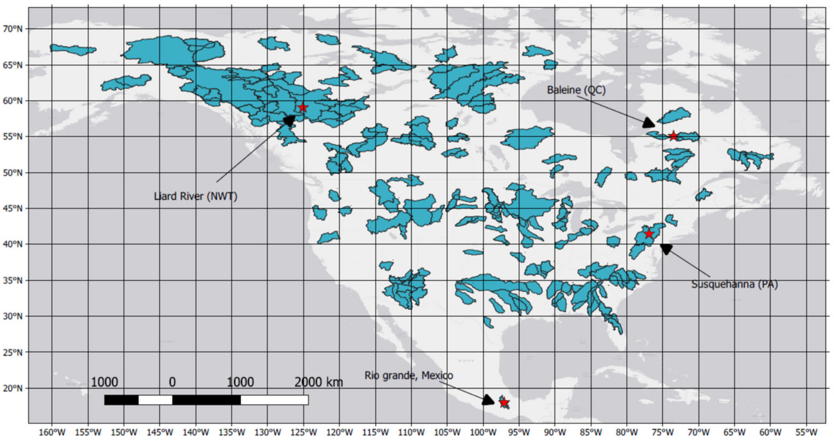
For this work, given the requirement for the gHM-gridded discharge values, large-sized catchments with a drainage area of more than 10,000 km² were selected. This 10,000 km² threshold was selected to ensure that discharge at the basin outlets was composed of at least a few runoff grid points that could be routed to the outlet, allowing us to attenuate the impacts of scale between catchments and the runoff generation scale. The study area is thus composed of 198 catchments across NA, with a drainage area between 10,000 and 508,000 km², an elevation ranging from 23 to 2171 m, and a slope of 0.4° to 20.3°. The annual average daily temperature ranges from −14 to + 22 °C, and the annual average precipitation varies from 127 to 1538 mm. The selected catchments are unregulated (or can be considered as such due to weak regulation). Figure 2 shows the location of the catchments over the study domain.

2.2. Global Hydrological Simulations from the ISIMIP Database

The present study is conducted in the framework of a research project through a partnership with NA water industries and the Ouranos Consortium (https://www.ouranos.ca/en/ accessed on 1 November 2021). In that project, the ISIMIP2a database is only explored.

Among the 13 gHMs participating in ISIMIP2a, 4 gHMs, namely, DBH [39], H08 [40], LPJml [41], and PCR-GLOBWB [42], are used to ensure a comparison with the rHM simulations (presented in Section 2.3) over the 1971–2010 period. Each gHM is driven by four global daily gridded meteorological datasets for a total of 16 gHM/driver combinations per catchment.

The four global daily gridded meteorological datasets used within the ISIMIP2a database are briefly presented in

Table 1. Description of the four meteorological datasets used to drive the gHMs. These datasets are distributed by the ISIMIP within the 2a phase.

Global Data	Reanalysis	Bias Correction	Grid Spatial Resolution	Period	Reference
GSWP3	20th Centurya	GPCC V6, GPCP, CRU and SRB	0.5° (~50km)	1901–2010	[43]
Princeton PGMFD v2	NCEP/NCAR Reanalysis 1	CRU, SBM and TRMM	0.5° (~50km)	1901–2012	[44]
WATCH Forcing Data (WFD)	ERA-40	GPCC v4	0.5° (~50km)	1971–2001	[45]
WFDEI.GPCC	ERA-Interim	GPCC v5 and v6	0.5° (~50km)	1979–2012	[46]

. All datasets are used to drive the gHMs. As WFDEI.GPCC starts in 1979, WFDEI combines WATCH (before 1979) and WFDEI.GPCC (after 1979) in ISIMIP2a.

The four gHMs are selected as they are the only ones available that contain the varsoc socio-economic scenario for the four global meteorological forcing datasets. The varsoc scenario includes changes in climate, population, gross domestic product (GDP), land use, technological progress, and other variables to reflect as best as possible the state of the world in the historical period [47,48]. This socio-economic scenario should be more representative than naturalized runs or those with a fixed present-day socio-economic scenario. All gHMs are run at the daily time step with a regular grid spatial aggregation, and they cover the globe at a spatial resolution of 0.5° (~50 km). A short description of each gHM, including model settings, specifications, and main hydrological processes, is provided in

Table 2. Characteristics of the four gHMs used in this study. Each gHM, at the beginning of 1971, was stabilized (spin-up) using pre-1970 data. (a) See [49] for the DDM30 data used for the river routing in DBH, H08, and LPJml. Note that the energy balance for estimating snowmelt simulates energy and mass exchanges between internal layers of the snowpack as well as snowpack stratigraphy from physically based calculations using simulated meteorological data.

gHM	Spin-Up	River Routing	PET Method	Snowmelt Method	Calibration
DBH	20-year	Linear reservoir based on DDM30 (a)	Energy balance [50]	Energy balance	No
H08	70-year	Linear reservoir based on DDM30 (a)	Bulk formula [40]	Energy balance	No
LPJml	5000-year potential natural vegetation spin-up, followed by 390-year land-use spin-up, both recycling 120-year random climate sequence	Linear reservoir based on DDM30 (a)	Priestley-Taylor [51]	Degree-day with precipitation factor	No
PCR–GLOBWB	50-year	Travel-time routing	Hamon [52]	Degree-day with rain–snow transition	No

. For a full technical description of the ISIMIP2a protocol and simulation data from the water (global) sector, see [47,48].

For each of the 198 study catchments, gHM-simulated discharge is obtained by selecting the value of the grid point with the maximum discharge (variable ‘dis’ in ISIMIP2a) within the catchment boundaries for each day. This allows comparisons of the gauged discharge values at the catchment outlet.

2.3. Regional Hydrological Simulations Based on the HYSETS Database

Two rHMs driven by the Princeton PGMFD v2 daily gridded meteorological dataset are used as a reference to compare the performance of the ISIMIP2a gHMs to site-specific rHMs, a necessary step towards meeting the objective of this study. It is thus expected that the rHM performance in simulating discharges will be better than that of the gHMs.

The selected rHMs are GR4J (modèle du Génie Rural à 4 paramètres Journaliers—a daily rural engineering model with four parameters; [53]) and HMETS (Hydrological Model of École de technologie supérieure; [54]), two lumped models operating at the daily time step. They have been widely used for various water-related purposes [55,56,57]. A short description of the main characteristics of the rHMs is provided in

Table 3. Characteristics of the two rHMs used in this study. Each rHM, at the beginning of 1971, was initialized (spin-up) using pre-1970 data (1-year spin-up based on the Princeton data).

rHM	Model Parameters (Nb.)	Input Data	Spin-Up	Flow Schemes	PET Method	Snowmelt Method	Calibration/Validation
GR4J	4	P, PET	1-year	Production and routing components	Oudin [58]	Degree-day (CEMANEIGE; [59])	Yes
HMETS	21	P, T	1-year	Two connected reservoirs for the saturated and vadose zones	Oudin [58]	Degree-day [60]	Yes

.

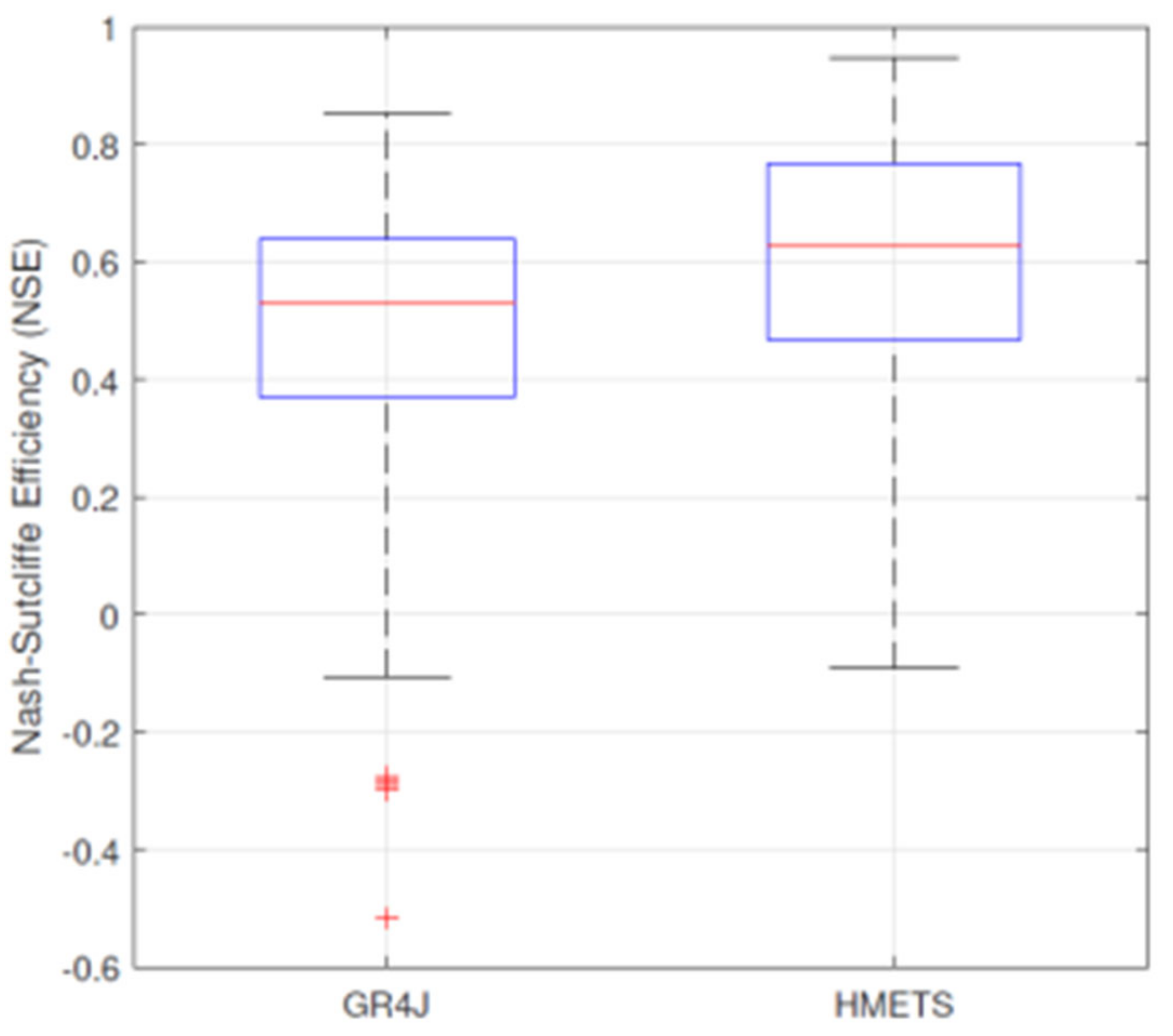
The first step is to calibrate the two rHMs for the 198 catchments with the Princeton PGMFD v2 dataset (https://esg.pik-potsdam.de/search/isimip/ accessed on 1 November 2021) and the HYSETS hydrometric data. Climate data is averaged at the catchment scale using an unweighted average of all grid points within each catchment boundary [38]. The calibration period is made over the first 20 years (1971–1990), whereas the validation is done based on the remaining 20 years (1991–2010). The parameters of the rHMs, which include the snowmelt module parameters, are calibrated with observed daily discharge data. Automatic calibrations are performed with different combinations of model parameters, and the optimal combination of parameter values is selected based on the objective function. The Shuffled Complex Evolution optimization algorithm, developed at the University of Arizona (SCE-UA), is used to obtain optimal parameter values for the rHMs [61]. SCE-UA is an evolutionary type of black-box optimization algorithm. A study [62] has shown that it is a proper calibration algorithm for small optimization problems such as those in this study. To ensure convergence, 15,000 objective function evaluations were permitted. The objective function used is the Nash-Sutcliffe Efficiency (NSE) metric [63] as it is the most well-known continuous discharge performance measure and is adequate, in most cases, over long time series. Figure 3 shows the validation NSE values for each rHM for all catchments combined. In all cases, as expected, the rHMs perform satisfactorily, with median NSE values exceeding 0.5. HMETS had slightly better performance (median NSE values of 0.62) than GR4J (median NSE values of 0.52) at simulating daily discharges over the 1991–2010 validation period. The results in the calibration period are similar to those in the validation period and are not shown here.

2.4. Model Performance and Statistical Criteria

For both the gHMs and rHMs, the simulated daily discharge time series are analyzed over the 1971–2010 period. The suggested metrics in the ISIMIP2a protocol model evaluation are the Nash-Sutcliffe Efficiency (NSE; [63]; Equation (1)) and the percent bias (PBIAS in %; Equation (2)), given by:

$$NSE=1-\left[\frac{{{\displaystyle \sum }}_{i=1}^N{\left(O_i-S_i\right)}^2}{{{\displaystyle \sum }}_{i=1}^N{\left(O_i-\overline{O}\right)}^2}\right]$$

(1)

$$PBIAS=\left[\frac{{{\displaystyle \sum }}_{i=1}^N\left(O_i-S_i\right)}{{{\displaystyle \sum }}_{i=1}^N{O}_i}\right]\times 100$$

(2)

where $O_i$ refers to the observed discharge for day i; $\overline{O}$ is the mean daily observed discharge; $S_i$ is the simulated discharge for day i; and N is the number of observed or simulated discharge values.

They are used in this study to evaluate the overall performance of both gHMs and rHMs with respect to the observations at the weekly time step for the whole period. A weekly time step is considered to minimize the impact of timing issues with gHMs, whose internal routing schemes are often too coarse to generate well-timed flow events. These metrics are also used to assess the quality of the high-flow and low-flow simulations by the gHMs and the rHMs, as they are common evaluation criteria for mean seasonal dynamics. Performance of both gHMs and rHMs are judged “satisfactory” for the weekly discharge simulations at the catchment-scale if NSE > 0.50 and relative bias ≤ ±25% (partly based on [64]). The NSE and relative bias values in evaluation are important since poor performance should limit the ability of the gHM–climate–dataset combinations to produce reliable trends for climate change impact studies.

3. Results

3.1. gHM Performance in Simulating Discharge at the Catchment Scale

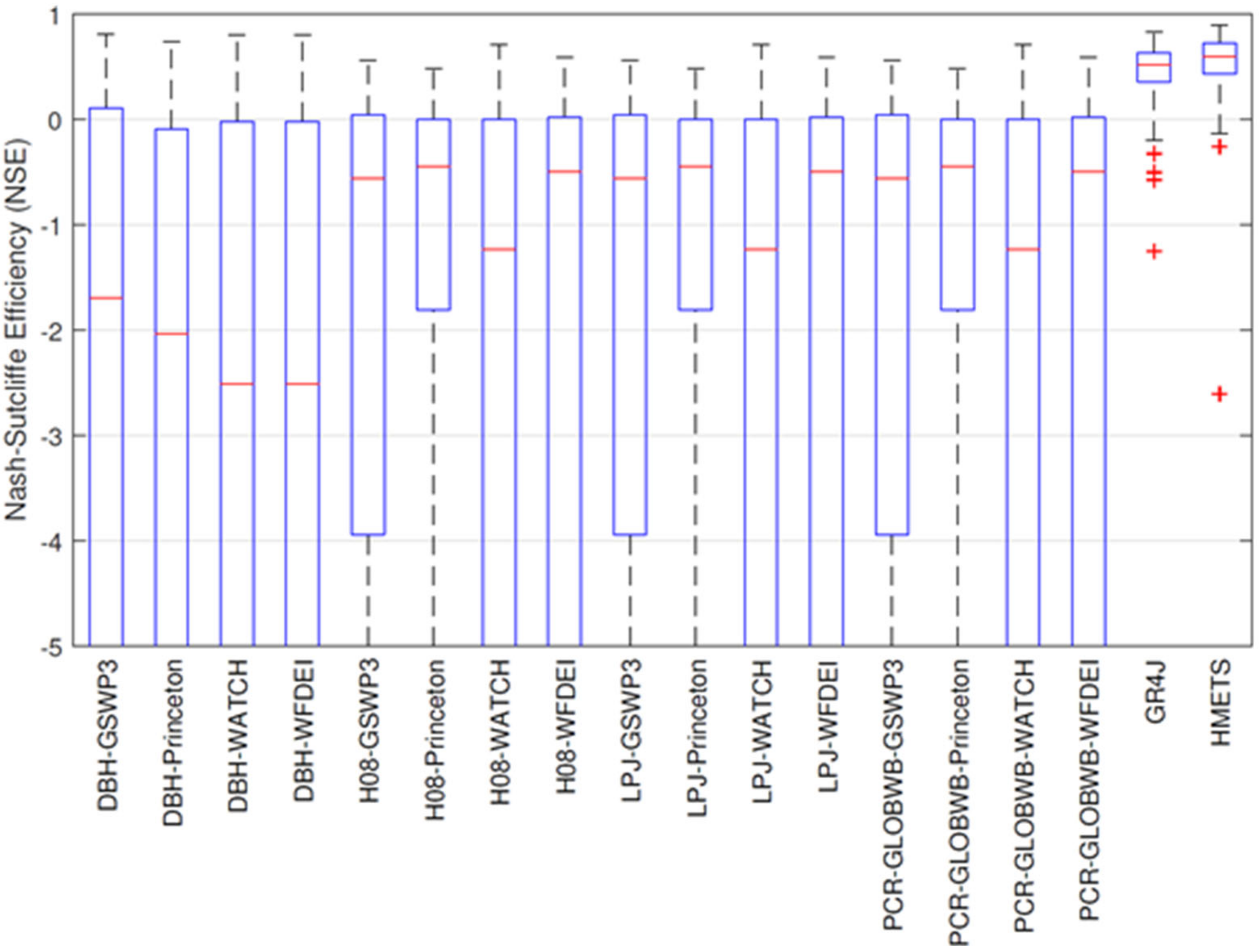
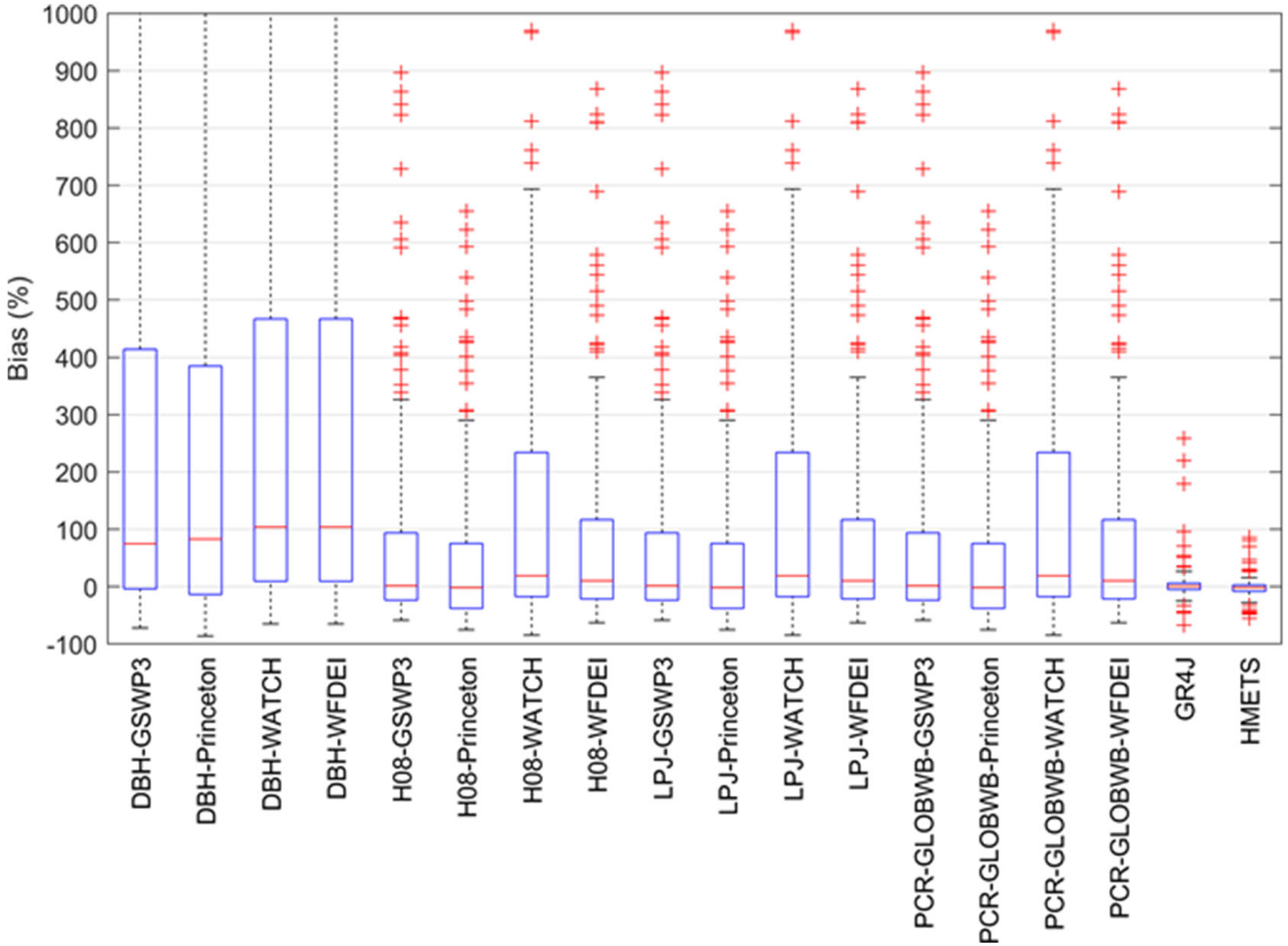
gHM performance in simulating discharge is measured by comparing it to that of the two rHMs taken individually for the 198 catchments over the 1971–2010 period, except for the gHM–WATCH combination, where the evaluation period is 1971–2001 due to WATCH data availability (see Table 1). Figure 4 shows the average NSE values of the discharge for the 16 gHM–climate–dataset combinations and the two rHMs. The same approach is utilized on the PBIAS metric, which is often used in operational reservoir management. Figure 5 shows the PBIAS values for the gHM–climate–dataset combinations and the two rHMs. The box-and-whisker plots are based on the 198 catchments.

From Figure 4, the gHMs perform poorly in simulating the discharge at the catchment scale, with negative median NSE values; the 25th–75th quantile boxes are practically below zero level in all cases. DBH displays the poorest performance whatever the global meteorological dataset used to drive the gHM. The gHM–Princeton combination generates lower variability in the simulated discharge values, as depicted by the box plot amplitude. Statistically, the gHM–WATCH combination performs the worst, with considerable uncertainty in the results. To test if it could be attributed to the different evaluation periods between WATCH and the other datasets, we computed the NSE values for all gHM–climate–dataset combinations for the 1971–2001 period. The results showed no significant improvement of gHM performance over the common period (not presented here). As expected, both rHM–Princeton combinations outperform all the gHM–climate–dataset combinations, with satisfactory median NSE values (NSE > 0.5).

Compared to the gHMs, both rHMs offer the best performance, with satisfactory bias values (PBIAS ≤ +25%) while decreasing the spread of the discharge values.

3.2. Detailed Analysis of four NA Catchments

To further understand the limitations of the global-scale simulations for catchment-scale hydrological studies, four catchments with contrasting climate features according to the Köppen climate classification and geomorphological features (drainage area, altitude) were analyzed; these sites were chosen among the large sample of catchments to be representative of the typical performance of all hydrological models involved. The location of each catchment is shown in Figure 2.

Table 4. General characteristics of the four NA catchments.

River Basin	Province or State (Country)	Drainage Area (km2)	Mean Altitude (m)	Köppen Climate cClassification
Baleine	Quebec (Canada)	32,500	380	Continental—Subarctic climate (Dfc)
Liard	Northwest Territories (Canada)	275,000	980	Continental—Subarctic climate (Dfc)
Rio Grande	Oaxaca (Mexico)	11,982	1869	Tropical—Tropical rainforest/monsoon climate (Af/Am)
Susquehanna	Pennsylvania (US)	67,313	410	Continental—Warm-summer humid continental climate (Dfb)

lists some of their main features. For all river basins, the catchment-scale climate inputs and discharge variables were examined.

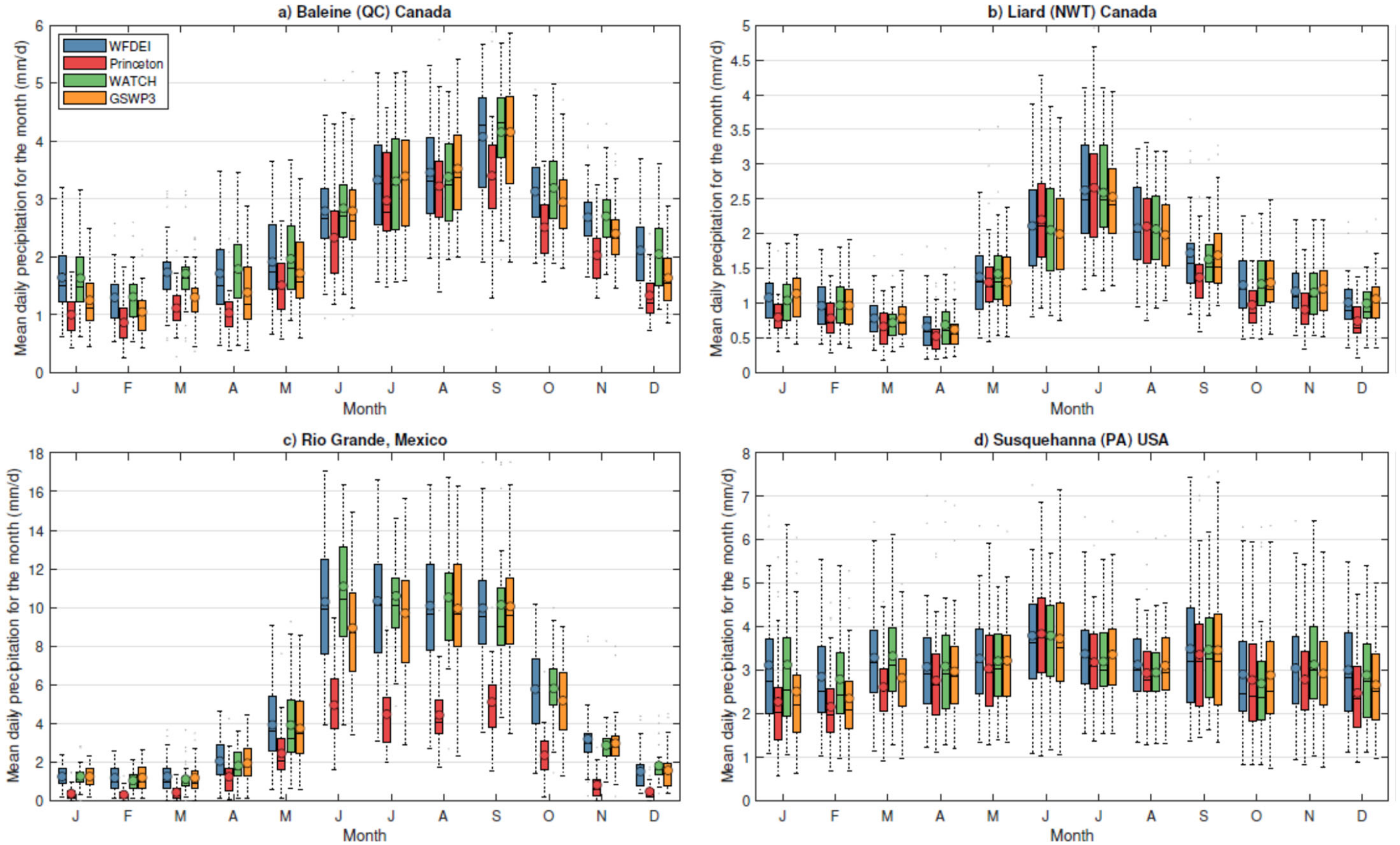
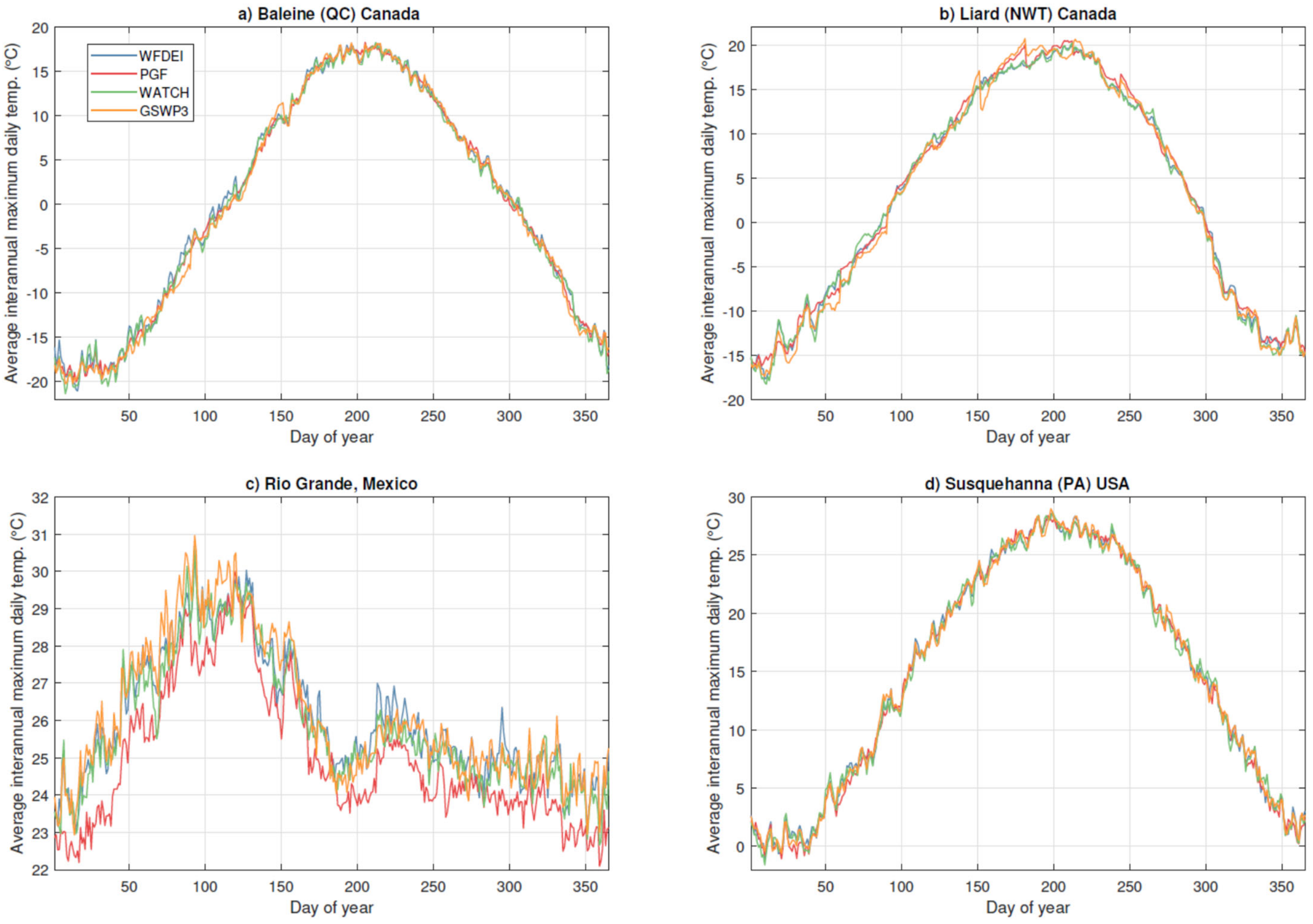
The characteristics of global meteorological forcing were investigated over the entire period (1971–2010) for daily precipitation (Figure 6), daily maximum (Figure 7), and minimum (Figure 8) temperatures. For precipitation, the mean interannual cycles differed significantly between the four datasets at the catchment scale, with the major discrepancies observed for the less rainy months (autumn and winter months). The highest differences in precipitation among the four global meteorological datasets were seen for the high-elevation Mexican catchment; the Princeton dataset showed an different overall pattern of mean daily precipitation over that catchment, with a lower precipitation amount throughout the year (Figure 6c). Fewer inter-dataset differences were observed in the mean interannual cycles of maximum and minimum temperatures. The four global meteorological forcings are, overall, in good agreement over the catchments, except for the high-elevation Mexican catchment, where the strongest variability in temperature is observed; again, for the Rio Grande River Basin, the Princeton dataset generates a different pattern compared to the other three datasets with colder temperatures Figure 7c and Figure 8c).

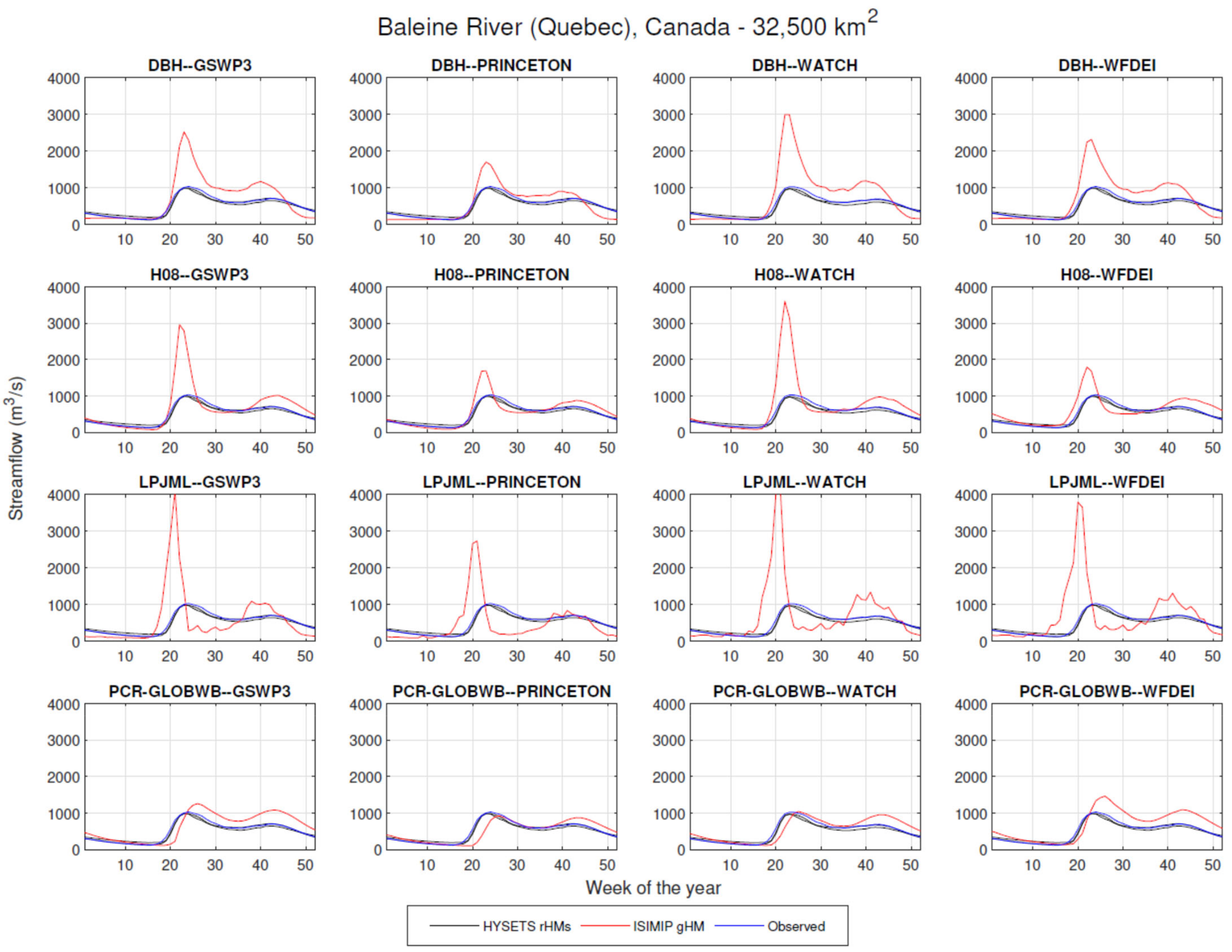
The ability of each gHM–climate–dataset combination to simulate catchment-scale discharge was then assessed by visual hydrograph comparison (Figure 9 and Figures S1, S3 and S5), through the analysis of the Taylor diagrams, which provide a summary of the relative skill of the gHMs (Figure 10 and Figures S2, S4 and S6), and of statistic criteria for the high- and low-flow periods (

Table 5. PBIAS values (%) of high and low flows computed for each gHM–climate–dataset combination and the two rHMs for the four catchments over the 1971–2010 period. The satisfactory PBIAS values are in bold (PBIAS ≤ ±25%; see Section 2.4).

River Basin	Global Meteorological Datasets	gHM						rHM
		DBH		H08	LPJml	PCR-GLOBWB	All gHMs	GR4J	HMETS
Bias high flows (%)—50% of highest observed flows
Baleine (S = 32,500 km2)	GSWP3	52		38	18	24	33	−11	−5
	Princeton	17		9	−13	−6	2
	WATCH	69		48	31	7	39
	WFDEI	53		14	25	34	32
	All datasets	47.8		27.3	15.3	14.8
Liard (S = 275,000 km2)	GSWP3	353		197	33	109	173	−10	−0.2
	Princeton	331		187	18	99	159
	WATCH	453		231	50	70	201
	WFDEI	421		193	45	118	194
	All datasets	390		202	37	99
Rio Grande (S = 11,982 km2)	GSWP3	−36		−52	−49	23	−29	−17	−10
	Princeton	−52		−48	−56	19	−34
	WATCH	−54		−61	−57	13	−40
	WFDEI	−61		−64	−62	17	−43
	All datasets	−51		−56	−56	18
Susquehanna (S = 67,313 km2)	GSWP3	−19		−31	−30	−28	−27	−9	−11
	Princeton	−30		−40	−37	−35	−36
	WATCH	−4		−7	−15	−29	−14
	WFDEI	−6		−14	−16	−19	−14
	All datasets	−15		−23	−25	−28
Bias low flows (%)—50% of lowest observed flows
Baleine (S = 32,500 km2)	GSWP3	0.4		13	7	38	15	20	4
	Princeton	−16		7	10	19	5
	WATCH	−6		16	62	27	25
	WFDEI	−0.5		51	78	46	43
	All datasets	−6		22	39	33
Liard (S = 275,000 km2)	GSWP3	206		946	951	630	683	104	−2
	Princeton	186		949	810	594	6345
	WATCH	235		982	1189	562	742
	WFDEI	237		1181	1137	671	807
	All datasets	216		1014	1022	614
Rio Grande (S = 11,982 km2)	GSWP3	−22		−81	−33	123	−3	73	49
	Princeton	−24		−78	−44	89	−14
	WATCH	−38		−88	−53	113	−17
	WFDEI	−53		−91	−53	110	−22
	All datasets	−34		−85	−46	109
Susquehanna (S = 67,313 km2)	GSWP3	224		−8	41	25	71	38	37
	Princeton	220		0.06	45	24	72
	WATCH	276		16	59	17	92
	WFDEI	255		12	52	41	90
	All datasets	244		5	49	27

and

Table 6. NSE values of high and low flows computed for each gHM–climate–dataset combination and the two rHMs for the four catchments over the 1971–2010 period. The satisfactory NSE values are in bold (NSE > 0.5; see Section 2.4).

River Basin	Global Meteorological Datasets	gHM					rHM
		DBH	H08	LPJml	PCR-GLOBWB	All gHMs	GR4J	HMETS
NSE high flows—50% of highest observed flows
Baleine (S = 32,500 km2)	GSWP3	−8.2	−11.7	−30.5	−2.1	−13.1	0.01	0.4
	Princeton	−1.7	−2.5	−16.7	−0.9	−5.5
	WATCH	−13.7	−18.0	−31.9	−0.6	−16.1
	WFDEI	−7.8	−4.7	−27.8	−2.7	−10.8
	All datasets	−8	−9	−27	−2
Liard (S = 275,000 km2)	GSWP3	−54.9	−15.2	−7.5	−3.8	−20.4	0.5	0.7
	Princeton	−47.6	−12.7	−5.0	−3.3	−17.4
	WATCH	−88.6	−20.0	−7.7	−1.6	−29.5
	WFDEI	−80.6	−14.0	−7.5	−4.9	−26.8
	All datasets	−67.9	−15.5	−6.9	−3.4
Rio Grande (S = 11,982 km2)	GSWP3	−3.6	−3.0	−2.6	−2.7	−2.9	−0.04	0.3
	Princeton	−1.0	−1.2	−1.1	−1.1	−1.1
	WATCH	−1.3	−2.0	−1.4	−1.1	−1.5
	WFDEI	−1.5	−2.0	−1.3	−1.0	−1.45
	All datasets	−1.9	−2.1	−1.6	−1.5
Susquehanna (S = 67,313 km2)	GSWP3	−0.6	−0.2	0.04	−0.1	−0.22	0.4	0.4
	Princeton	−0.6	−0.3	−0.1	−0.3	−0.33
	WATCH	−1.1	−0.03	0.2	−0.1	−0.26
	WFDEI	−1.1	−0.1	0.2	−0.2	−0.3
	All datasets	−0.9	−0.2	0.1	−0.2
NSE low flows—50% of lowest observed flows
Baleine (S = 32,500 km2)	GSWP3	−3.5	−1.1	−26.6	−1.4	−8.2	0.2	0.4
	Princeton	−2.2	−0.4	−28.5	−0.3	−7.9
	WATCH	−4.0	−1.6	−59.0	−0.5	−16.3
	WFDEI	−3.2	−2.3	−66.3	−1.9	−18.4
	All datasets	−3.2	−1.4	−45.1	−1
Liard (S = 275,000 km2)	GSWP3	−222.8	−1043.8	−3438.1	−360.6	−1266	−12	−0.8
	Princeton	−198.2	−1028.8	−2095.0	−318.2	−910
	WATCH	−272.4	−1112.9	−3309.3	−264.0	−1239
	WFDEI	−292.0	−1483.4	−3179.2	−412.1	−1341
	All datasets	−246.4	−1167.2	−3005.4	−338.7
Rio Grande (S = 11,982 km2)	GSWP3	−21.4	−8.7	−22.3	−23.9	−19.1	−6.6	−6.7
	Princeton	−12.5	−6.8	−8.9	−16.9	−11.3
	WATCH	−9.0	−8.0	−9.9	−19.3	−11.6
	WFDEI	−6.7	−6.8	−9.2	−15.0	−9.4
	All datasets	−12.4	−7.6	−12.6	−18.8
Susquehanna (S = 67,313 km2)	GSWP3	−32.6	−1.1	−3.0	−2.1	−9.7	−1.6	−2.4
	Princeton	−31.4	−1.3	−3.3	−1.6	−9.4
	WATCH	−57.2	−2.1	−6.0	−2.4	−16.9
	WFDEI	−47.3	−2.4	−5.3	−4.0	−14.8
	All datasets	−42.1	−1.7	−4.4	−2.5

). For the Baleine River Basin, the comparison of the gHM–climate–dataset combinations with the observations and the rHMs shows significant differences in the reproduction of the mean interannual cycles of the simulated discharge (Figure 9 and Figure 10). Most of the gHM–climate–dataset combinations display spatial correlation coefficients above 0.6, except for the LPJml, with high RMSVD values (Figure 10). The high flow period is overestimated in all the DBH–dataset combinations (Figure 9 and Table 5). In the H08 simulations, an overestimation of the peak flow is present regardless of the dataset used to drive the gHM. The peak flow is both overestimated and delayed in all the LPjml simulations; however, there are more satisfactory bias values for the high flow period (Table 5). PCR–GLOBWB and H08 provide more realistic discharge patterns and variability than DBH and LPJml (Figure 10). In particular, the PCR–GLOBWB–Princeton and PCR–GLOBWB–WATCH combinations almost capture both the magnitude and timing of the peak flow, which translate into acceptable relative bias values of high flows (Table 5); both the PCR–GLOBWB–Princeton and PCR–GLOBWB–WATCH combinations are the closest to the rHM simulations (Figure 9). Most of the gHM–climate–dataset combinations give satisfactory bias values for the low flows (Table 5).

For the Liard River Basin, all the DBH and H08 simulations depict an overly vigorous mean interannual cycle of discharge with overestimated high flows (Figure S1 and Table 5). Most of the gHM–climate–dataset combinations display correlation coefficients above 0.6 but with high standard deviation and RMSD values (Figure S2). The magnitude of the spring peak flow is consistently overestimated in the LPJml simulations, with a similar time offset whatever the dataset used as forcing. Such finding is observed for both river basins submitted to a subarctic climate (Table 4). The misrepresentation of the spring peak flow is linked to the misrepresentation of the snowmelt peak, caused either by a cold bias in temperature or poor representation of snow processes by the gHM. Since all global meteorological datasets give similar patterns of air temperature and the other gHMs do not provide delayed spring peak flow, we attribute that to the snowpack state processing into LPJml, which relies on a degree-day approach with a precipitation factor (Table 2). All the PCR–GLOBWB–dataset combinations give smooth mean interannual cycles of the simulated discharge, with strong relative bias values of high and low flows (Table 5).

As for the Rio Grande River Basin, the mean interannual cycle of discharge is captured by any gHM–climate–dataset combination (Figure S3). LPJml displays the poorest model skill for this catchment. H08 and PCR–GLOBWB display the highest correlation coefficient values and the lowest standard deviation and RMSD values for this catchment (Figure S4). Both the high and low flows tend to be underestimated by the gHMs (except for PCR–GLOBWB), with significant bias values (Table 5). Given the similar high flow underestimation by DBH, H08, and LPJmL, when driven by the four global meteorological datasets (Figure S3), but depicting marked discrepancies in seasonal climate patterns over that high-elevation catchment (Figure 7, Figure 8 and Figure 9), the systematic underestimation of the high-flow period seems to be more related to the internal pathways of the gHMs for depicting hydrological processes, such as PET (Table 2), rather than the quality of the global meteorological datasets. The errors in simulating weekly low flows, particularly perceptible on the DBH, H08, and LPJmL simulations, are linked to the challenges faced by the gHMs in accurately representing groundwater and baseflow processes. The rHMs reproduced the overall seasonal cycle of discharge for this catchment, with correlation coefficients above 0.6 (Figure S4); however, the low flows are overestimated, and the magnitude of the peak flow is consistently underestimated (Figure S3 and Table 5).

Regarding the Susquehanna River Basin, the gHM–climate–dataset combinations perform poorly in reproducing seasonal discharge (Figure S5) and systematically provide a time offset of the spring peak flow. This is confirmed with the analysis of the Taylor diagram with strong RMSD values (Figure S6). H08, DBH, and PCR–GLOBWB tend to better capture the mean interannual cycles of discharge, with a good simulation of low flows with minimal bias values, especially for the H08–dataset and PCR–GLOBWB–dataset combinations (Table 5). Only H08, when driven by WATCH and WFDEI, exhibits realistic peak flow simulations that are the closest to the rHM simulations.

As for the gHM–rHM comparison, the rHM–Princeton combinations yield more consistent discharge simulations over the catchments than the gHM–Princeton combinations, with a more reliable reproduction of the observed magnitude and timing of peak flow (Figure 9 and Figures S1, S3 and S5), and better model skill. The standard deviation values of the rHMs are similar to the observations, with higher correlation coefficient values and lower RMSD values than the gHMs (Figure 10 and Figures S2, S4 and S6). This confirms the fact that the gHMs, with their coarse resolution and the related limitations regarding the misrepresentation of local topography, translate into some unrealistic simulations of discharge for the four NA catchments. However, a general underestimation of the rHM-simulated high flows is observed, while the low flows are generally overestimated. This might be explained by the inadequate representation of the seasonal PET cycle, which is likely underestimated during the high flow period and overestimated during the low flow period. This is likely related to the potential bias in the global meteorological data showing their limitations of use for hydrological modeling at the catchment scale.

3.3. Potential Factors Controlling gHM Performance

To explain the gHMs’ poor ability to simulate discharge at the catchment scale, two levels of issue that can impact model efficiency are explored. For the four catchments, we questioned the impact of the geomorphological features (catchment size, altitude, geographical location) as well as the global meteorological forcing.

We investigated the influence of the geomorphological features on the PBIAS and NSE values of high flows and low flows for each gHM and for the two rHMs by considering all meteorological datasets combined (Table 5 and Table 6). The results show that the poorest gHM performance at simulating seasonal flows are obtained for the Liard River Basin in the northwest territories (Canada), followed by the Rio Grande River Basin in Oaxaca (Mexico), which are the highest elevation catchments and the largest (S = 325,000 km²) and the smallest (S = 11,982 km²) sized catchments, respectively, among the four sites. All gHMs lead to a significant overestimation of seasonal flows for the Liard River Basin and a significant underestimation of seasonal flows for the Rio Grande River Basin, with negative NSE values in both cases. For the Baleine and Susquehanna River Basins, the two northeastern NA catchments with a mean altitude below 500 m and a drainage area between 30,000 and 70,000 km², the overall gHM performance at simulating seasonal flows is slightly improved, especially for the high flows in terms of PBIAS only. Even though the geomorphological features of the catchments contribute to the gHM performance, this improvement remains minor. The same finding can be transposed to the two rHMs since the values of statistical criteria do not significantly increase with any geomorphological features.

We then investigated the influence of the global meteorological forcing on the PBIAS and NSE values of high flows and low flows by comparing each global dataset for all gHMs combined and the two rHMs (Table 5 and Table 6). Results show that the gHM–dataset combinations lead to significant bias in the high-flow simulations, with some sparse exceptions such as the gHM–Princeton combination for the Baleine River Basin as well as the gHM–WATCH and gHM–WFDEI combinations for the Susquehanna River Basin. As for the low flows, all gHM–dataset combinations tend to provide more reliable simulations over the Baleine and Rio Grande River Basins, while they fail at producing acceptable results in terms of relative bias over the Liard and Susquehanna River Basins. There is, thus, no global driving dataset that consistently outperforms others locally for seasonal flow simulations when they are used as inputs to the gHMs. However, both rHMs, forced by the Princeton dataset, led to improved simulations of seasonal flows, with more acceptable values of PBIAS and NSE.

4. Discussion

4.1. On the Use of gHMs and rHMs Driven by Global Meteorological Datasets

When looking at the NA region, we found some variability between the global driving datasets for the 198 catchments combined (Figure 4 and Figure 5). The use of Princeton in the gHM–climate–dataset combinations leads to more consistent discharge simulations with reduced error. However, when looking at the scale of the specific site, the gHMs used in this study do not appear to be sensitive to the choice of the global meteorological datasets since the datasets lead to similar levels of efficiency in terms of discharge simulations (Table 5 and Table 6). At the local scale, a higher variability between the gHMs is observed, as compared to the inter-dataset variability (Figure 9 and Figure 10). The driving forcing datasets seem to have more influence regionally than at the catchment scale, where, locally, even though the global driving datasets display some discrepancies in seasonal climate patterns, especially for precipitation (Figure 6, Figure 7 and Figure 8), the differences would be more linked to the way the gHMs represent the main hydrological processes and their resolution.

However, the moderate performances of the rHM–Princeton combinations for the four catchments, especially for the high-elevation catchment, point to limitations in global data quality, which seriously constrain any efforts at hydrological modeling for the NA region, as is the case for the Southern Africa region [65]. Disentangling the factors explaining the poor quality of the global meteorological datasets is not easy as more than one characteristic differs between each dataset (e.g., bias correction, reanalysis; see Table 1). Many studies have reported the importance of incorporating observational or pseudo-observational (satellite remote sensing data, radar data) inputs into global meteorological products to better depict spatiotemporal climate variability in complex areas [66,67]. One study [68] compared seven global datasets in five Köppen climate zones and underlined that there are some global datasets that perform well under a specific climate but that no single one performs best for all climate types. Another study [69] showed that the WFDEI dataset only provides better discharge simulations than reanalysis in the subtropical and humid continental climate regions.

Using global meteorological datasets for hydrological modeling, such as in ISIMIP2a, relies on pragmatic reasons (e.g., spatiotemporal resolution, period of available datasets). Global dataset intercomparisons for choosing the most reliable products are often set aside due to the time constraints in such large projects. However, conducting an evaluation of global meteorological dataset quality before using them as forcings to the gHMs is required, especially when the rHMs are also driven by the global datasets, leading to a low level of efficiency in terms of discharge simulations at the catchment scale.

4.2. gHMs’ Performance between Catchments

We find a high variability between gHMs in their ability to reproduce the mean interannual cycles of weekly discharge for the four catchments. This confirms findings from previous catchment-scale studies that emphasize that large spreads from the gHMs are not primarily due to errors in the driving data or local geomorphological aspects but to errors in the gHM structure [32,70]. The gHM models include quite simple linear reservoir approaches to routing flows to the outlet. In addition, the DEM resolution used in the gHM models cannot precisely reflect the flow path in complex regions, such as the mountain catchments. Misrepresentations of physical processes can explain the discrepancies between the gHM-simulated and observed (or rHM-simulated) discharges, which are more obvious at the catchment scale than over a continental region such as the NA region. For instance, the overestimated high flows in the fall over the Rio Grande River Basin by most gHMs can be a result of lower PET. The PET simulations were shown to feature large variations between the ISIMIP2a gHMs [71]. Another factor could be the inability of the gHMs to accurately represent soil properties, thus influencing the generation and timing of high flows [72]. Over the Baleine and Liard River Basins, all gHMs fail to capture the spring peak flow. The poor snowmelt simulation is likely the main reason for such a bias. Temporal biases in snow-dominant regions have been reported [73,74,75], largely due to driving data errors and the misrepresentation of snow processes (e.g., meltwater infiltration into soil profiles, refreezing of meltwater over cold periods), and snowmelt delays in the gHMs [76].

When aggregating across catchments, no gHM stands out in the reproduction of discharge for the set of specific sites (Figure 9, Figure 10 and Figures S1–S6). This is partly explained by both the generalized parameters and the relatively coarse resolution of the ISIMIP2a gHMs, which prevent them from performing accurately in different locations under different climates. In addition, when driven by different global meteorological datasets, the performance of a given gHM (for instance, PCR–GLOBWB in Figure 9 and Figures S1, S3 and S5) is relatively similar. However, for a given driving dataset (for instance, WFDEI in Figure 9 and Figures S1, S3 and S5), the differences in the gHM structure and parametrization lead to highly contrasted reproductions of mean flow seasonal dynamics between the gHMs.

In hydrological modeling, an increase in model efficiency with the increasing size of catchments is often reported [77]. Ref. [78] showed that the drainage area of the catchment is one of the five most significant explanatory variables affecting the discharge simulations. It is expected that for large catchments with a smooth hydrological behavior, it will be easier for the models to reproduce the discharge. This finding cannot be transposed to both the gHMs and rHMs in the present study (Table 5 and Table 6). Moreover, the meteorological input data for large catchments are known with less uncertainty than for small catchments, which should tend towards a better gHM performance for larger catchments. Again, this is not illustrated in this work.

Multi-gHM intercomparison studies carried out over the last few years have revealed large differences among the gHMs [4,72]. It is crucial to identify error sources and to investigate why they exist to improve gHMs [6]. Therefore, caution should be applied in selecting only one gHM in catchment-scale hydrological applications. Considering more than one gHM appears to be a good option to account for the uncertainty associated with the gHM structure. In the case of the application of multiple gHMs in various locations, it could be tempting, yet unwise, to exclude the gHM with the weakest performance in the analysis, as there could be a risk of missing the other skills of that gHM for another location, as seen with PCR–GLOBWB in the present study.

4.3. gHM versus rHM Approach at the Catchment Scale

From the analysis of the 198 catchments combined, the comparison of discharge simulations by the gHMs and rHMs shows that the median NSE and error spread are not comparable (>50% difference: Figure 4, Figure 5 and Figure 6) and the bias values and errors spread are not comparable (>10% difference: Figure 4 and Figure 6).

From the analysis of the four specific sites, the comparison of discharge simulations by the gHMs and rHMs shows that no gHM can reproduce the observed mean seasonal dynamics. Both rHMs depict better skill (Figure 10 and Figures S2, S4 and S6) at simulating discharge variability as well as the magnitude and the timing of peak flows compared to the gHMs (Figure 9 and Figures S1, S3 and S5).

The better performance of rHMs compared to gHMs at the catchment scale is likely linked to: (a) better representation of snow processes (accumulation and melting), which is critical for peak flow dynamics in the Baleine and Liard River Basins; (b) better representation of groundwater and baseflow processes required for the low-flow simulations; and (c) the calibration of rHMs for each catchment (as compared to the uncalibrated gHMs), leading to better reproduction of the overall hydrological processes. Both rHMs driven by the Princeton dataset give better results than the gHM–Princeton combinations, and HMETS–Princeton combination provides more satisfactory discharge simulations than the GR4J–Princeton combination. The first finding can be explained by the existence of calibrated parameters in rHMs, allowing compensation of the errors in global datasets at the regional and local scale compared to the gHMs; the second finding is probably related to the number of model parameters since HMETS has a larger set of parameters compared to GR4J (23 calibrated parameters versus 4 calibrated parameters; Table 2), leading to a higher degree of freedom and better model adaptability to different regions.

Our findings are similar to those of [13], who compared simulations of several rHMs and gHMs for the Lena River Basin in Russia. The authors reported a high performance of the rHMs, partly attributed to their calibration. There is, thus, a compromise in continuing gHM applicability at the catchment scale and ignoring local diversity in the physiographic and climate features on each river basin. In practice, and for operational purposes, the gHMs with a spatial resolution of 0.5°, such as in the ISIMIP2a, cannot be the preferred option for catchment-scale applications. However, as mentioned in other studies [6,79,80], the gHMs are good candidates for valuable spatiotemporal estimation of global water resources and surface waters and for understanding human water uses and providing future trends of changes for those estimates. This is in clear contrast to the rHMs, which can be implemented on a specific site to respond to local water- and energy-related issues as they are designed for this purpose.

5. Conclusions

This study presents a catchment-scale comparative evaluation of the performance of four gHMs driven by four global meteorological datasets against two rHMs driven by one global meteorological dataset using two statistical criteria, Taylor diagrams, and visual hydrograph comparisons. We provide aggregated catchment-scale results, facilitating the comparison of model performance spatially for 198 large-sized catchments over the NA region. These findings are critical, as they provide the basis for the climate change impact studies using the gHMs in the next phase of ISIMIP2a.

We find a tendency for most gHM–climate–dataset combinations to overestimate discharges with negative NSE scores and large positive PBIAS and RMSD values. The errors and median values spread for the gHM-simulated discharges are not in good agreement with the observations or the rHM simulations. Looking at the four selected large-sized catchments, no gHM–climate–dataset combination can simulate the seasonal weekly discharge cycles. The magnitude and timing of the peak flows are poorly captured by most applied gHMs in the four catchments. Our evaluation provides recommendations to the global-scale hydrological modeling community in pursuing efforts to improve the gHMs’ ability to reproduce the global characteristics of discharge seasonality. The results obtained by considering the four forcing datasets slightly vary the conclusions drawn at the catchment scale; however, more influence seems to be associated with the gHM resolution and structure. Both the rHMs, driven by the global dataset, provide better simulation results for the 198 NA catchments in terms of the criteria used in this study.

This study evaluates gHM performance regarding river discharge for the NA region. We naturally recognize that a similar evaluation conducted in other regions will be welcome to confirm our findings. Further assessments, including other water balance components such as snowmelt and potential evapotranspiration, could provide more insights into the performance of the gHMs, particularly for the representation of seasonal dynamics at the catchment scale. In addition, extensive cross-validation of the rHMs driven by the ISIMIP2a global meteorological datasets, as well as the use of regionalized rHM parameters, might be considered in future work for providing further insights into rHM accuracy compared to that of the gHMs for large-sized catchments.

Our results show that there are still some challenges with accurate catchment-scale simulations of discharges by the gHMs. The gHMs, as implemented within ISIMIP2a, exhibited large uncertainties over the 1971–2010 period over the NA region. Therefore, a systematic and comprehensive evaluation of the gHMs within ISIMIP2a over a historical period is recommended before they are used for climate change impact studies. However, the rHM approach is found to be more reliable; we, therefore, recommend using it for catchment-scale hydrological studies, particularly where findings will be used to support operational decision-making.

Our study can be extended by comparing both ISIMIP2A and ISIMIP3a experiments and by evaluating if the ISIMIP3a models’ performance is improved regarding their counterparts by reducing uncertainty in the discharge simulations over NA catchments. Other statistical evaluation metrics and additional flow indicators could be included in such an assessment.

References

- Ruane, A.C.; Teichmann, C.; Arnell, N.W.; Carter, T.R.; Ebi, K.L.; Frieler, K.; Goodess, C.M.; Hewitson, B.; Horton, R.; Kovats, R.S.; et al. The Vulnerability, Impacts, Adaptation and Climate Services Advisory Board (VIACS AB v1.0) contribution to CMIP6. Geosci. Model Dev. 2016, 9, 3493–3515. [Google Scholar] [CrossRef] [Green Version]
- Nazemi, A.; Wheater, H.S. On inclusion of water resource management in Earth system models—Part 1: Problem definition and representation of water demand. Hydrol. Earth Syst. Sci. 2015, 19, 33–61. [Google Scholar] [CrossRef] [Green Version]
- Widén-Nilsson, E.; Halldin, S.; Xu, C.-Y. Global water-balance modelling with WASMOD-M: Parameter estimation and regionalisation. J. Hydrol. 2007, 340, 105–118. [Google Scholar] [CrossRef]
- Zaherpour, J.; Gosling, S.N.; Mount, N.; Schmied, H.M.; Veldkamp, T.I.E.; Dankers, R.; Eisner, S.; Gerten, D.; Gudmundsson, L.; Haddeland, I.; et al. Worldwide evaluation of mean and extreme runoff from six global-scale hydrological models that account for human impacts. Environ. Res. Lett. 2018, 13, 065015. [Google Scholar] [CrossRef]
- Sood, A.; Smakhtin, V. Global hydrological models: A review. Hydrol. Sci. J. 2015, 60, 549–565. [Google Scholar] [CrossRef]
- Masaki, Y.; Hanasaki, N.; Biemans, H.; Schmied, H.M.; Tang, Q.; Wada, Y.; Gosling, S.; Takahashi, K.; Hijioka, Y. Intercomparison of global river discharge simulations focusing on dam operation—Multiple models analysis in two case-study river basins, Missouri–Mississippi and Green–Colorado. Environ. Res. Lett. 2017, 12, 055002. [Google Scholar] [CrossRef] [PubMed]
- Krysanova, V.; Donnelly, C.; Gelfan, A.; Gerten, D.; Arheimer, B.; Hattermann, F.; Kundzewicz, Z.W. How the performance of hydrological models relates to credibility of projections under climate change. Hydrol. Sci. J. 2018, 63, 696–720. [Google Scholar] [CrossRef]
- Dankers, R.; Arnell, N.W.; Clark, D.; Falloon, P.D.; Fekete, B.M.; Gosling, S.; Heinke, J.; Kim, H.; Masaki, Y.; Satoh, Y.; et al. First look at changes in flood hazard in the Inter-Sectoral Impact Model Intercomparison Project ensemble. Proc. Natl. Acad. Sci. USA 2014, 111, 3257–3261. [Google Scholar] [CrossRef] [PubMed] [Green Version]
- Zhang, Y.; Zheng, H.; Chiew, F.H.S.; Arancibia, J.P.; Zhou, X. Evaluating Regional and Global Hydrological Models against Streamflow and Evapotranspiration Measurements. J. Hydrometeorol. 2016, 17, 995–1010. [Google Scholar] [CrossRef]
- Beck, H.E.; van Dijk, A.I.J.M.; de Roo, A.; Dutra, E.; Fink, G.; Orth, R.; Schellekens, J. Global evaluation of runoff from 10 state-of-the-art hydrological models. Hydrol. Earth Syst. Sci. 2017, 21, 2881–2903. [Google Scholar] [CrossRef] [Green Version]
- Krysanova, V.; Zaherpour, J.; Didovets, I.; Gosling, S.N.; Gerten, D.; Hanasaki, N.; Schmied, H.M.; Pokhrel, Y.; Satoh, Y.; Tang, Q.; et al. How evaluation of global hydrological models can help to improve credibility of river discharge projections under climate change. Clim. Chang. 2020, 163, 1353–1377. [Google Scholar] [CrossRef]
- Gädeke, A.; Krysanova, V.; Aryal, A.; Chang, J.; Grillakis, M.; Hanasaki, N.; Koutroulis, A.; Pokhrel, Y.; Satoh, Y.; Schaphoff, S.; et al. Performance evaluation of global hydrological models in six large Pan-Arctic watersheds. Clim. Chang. 2020, 163, 1329–1351. [Google Scholar] [CrossRef]
- Hattermann, F.F.; Krysanova, V.; Gosling, S.N.; Dankers, R.; Daggupati, P.; Donnelly, C.; Flörke, M.; Huang, S.; Motovilov, Y.; Buda, S.; et al. Cross-scale intercomparison of climate change impacts simulated by regional and global hydrological models in eleven large river basins. Clim. Chang. 2017, 141, 561–576. [Google Scholar] [CrossRef]
- Troin, M.; Arsenault, R.; Brissette, F. Performance and Uncertainty Evaluation of Snow Models on Snowmelt Flow Simulations over a Nordic Catchment (Mistassibi, Canada). Hydrology 2015, 2, 289–317. [Google Scholar] [CrossRef] [Green Version]
- Odusanya, A.E.; Mehdi, B.; Schürz, C.; Oke, A.O.; Awokola, O.S.; Awomeso, J.A.; Adejuwon, J.O.; Schulz, K. Multi-site calibration and validation of SWAT with satellite-based evapotranspiration in a data-sparse catchment in southwestern Nigeria. Hydrol. Earth Syst. Sci. 2019, 23, 1113–1144. [Google Scholar] [CrossRef] [Green Version]
- Mockler, E.M.; O’Loughlin, F.E.; Bruen, M. Understanding hydrological flow paths in conceptual catchment models using uncertainty and sensitivity analysis. Comput. Geosci. 2016, 90, 66–77. [Google Scholar] [CrossRef]
- Roy, T.; Serrat-Capdevila, A.; Gupta, H.; Valdes, J. A platform for probabilistic Multimodel and Multiproduct Streamflow Forecasting. Water Resour. Res. 2017, 53, 376–399. [Google Scholar] [CrossRef] [Green Version]
- Muhammad, A.; Stadnyk, T.A.; Unduche, F.; Coulibaly, P. Multi-Model Approaches for Improving Seasonal Ensemble Streamflow Prediction Scheme with Various Statistical Post-Processing Techniques in the Canadian Prairie Region. Water 2018, 10, 1604. [Google Scholar] [CrossRef] [Green Version]
- Troin, M.; Arsenault, R.; Wood, A.W.; Brissette, F.; Martel, J. Generating Ensemble Streamflow Forecasts: A Review of Methods and Approaches Over the Past 40 Years. Water Resour. Res. 2021, 57, e2020WR028392. [Google Scholar] [CrossRef]
- Arsenault, R.; Brissette, F. Multi-model averaging for continuous streamflow prediction in ungauged basins. Hydrol. Sci. J. 2016, 61, 2443–2454. [Google Scholar] [CrossRef] [Green Version]
- Zhang, L.; Lu, J.; Chen, X.; Liang, D.; Fu, X.; Sauvage, S.; Perez, J.-M.S. Stream flow simulation and verification in ungauged zones by coupling hydrological and hydrodynamic models: A case study of the Poyang Lake ungauged zone. Hydrol. Earth Syst. Sci. 2017, 21, 5847–5861. [Google Scholar] [CrossRef] [Green Version]
- Troin, M.; Velázquez, J.A.; Caya, D.; Brissette, F. Comparing statistical post-processing of regional and global climate scenarios for hydrological impacts assessment: A case study of two Canadian catchments. J. Hydrol. 2015, 520, 268–288. [Google Scholar] [CrossRef]
- Bodian, A.; Dezetter, A.; Diop, L.; Deme, A.; Djaman, K.; Diop, A. Future Climate Change Impacts on Streamflows of Two Main West Africa River Basins: Senegal and Gambia. Hydrology 2018, 5, 21. [Google Scholar] [CrossRef] [Green Version]
- Arsenault, R.; Essou, G.R.C.; Brissette, F.P. Improving Hydrological Model Simulations with Combined Multi-Input and Multimodel Averaging Frameworks. J. Hydrol. Eng. 2017, 22, 04016066. [Google Scholar] [CrossRef]
- Asadieh, B.; Krakauer, N.Y. Global change in streamflow extremes under climate change over the 21st century. Hydrol. Earth Syst. Sci. 2017, 21, 5863–5874. [Google Scholar] [CrossRef] [Green Version]
- Rakovec, O.; Kumar, R.; Kaluza, M.; Schweppe, R.; Thober, S.; Attinger, S.; Samaniego, L. Seamless Reconstruction of Global Scale Hydrologic Simulations: Challenges and Opportunities. Geophysical Research Abstracts 21 2019, EGU 2019-13125. Available online: https://meetingorganizer.copernicus.org/EGU2019/EGU2019-13125.pdf, (accessed on 25 February 2019).
- Zhou, X.; Zhang, Y.; Wang, Y.; Zhang, H.; Vaze, J.; Zhang, L.; Yang, Y.; Zhou, Y. Benchmarking global land surface models against the observed mean annual runoff from 150 large basins. J. Hydrol. 2012, 470, 269–279. [Google Scholar] [CrossRef]
- Gudmundsson, L.; Wagener, T.; Tallaksen, L.M.; Engeland, K. Evaluation of nine large-scale hydrological models with respect to the seasonal runoff climatology in Europe. Water Resour. Res. 2012, 48, 11504. [Google Scholar] [CrossRef]
- Hagemann, S.; Gates, L.D. Validation of the hydrological cycle of ECMWF and NCEP reanalyses using the MPI hydrological discharge model. J. Geophys. Res. Space Phys. 2001, 106, 1503–1510. [Google Scholar] [CrossRef]
- Towner, J.; Cloke, H.L.; Zsoter, E.; Flamig, Z.; Hoch, J.M.; Bazo, J.; de Perez, E.C.; Stephens, E.M. Assessing the performance of global hydrological models for capturing peak river flows in the Amazon basin. Hydrol. Earth Syst. Sci. 2019, 23, 3057–3080. [Google Scholar] [CrossRef] [Green Version]
- Nijssen, B.; O’Donnell, G.M.; Lettenmaier, D.P.; Lohmann, D.; Wood, E. Predicting the Discharge of Global Rivers. J. Clim. 2001, 14, 3307–3323. [Google Scholar] [CrossRef]
- Gudmundsson, L.; Tallaksen, L.M.; Stahl, K.; Clark, D.; Dumont, E.; Hagemann, S.; Bertrand, N.; Gerten, D.; Heinke, J.; Hanasaki, N.; et al. Comparing Large-Scale Hydrological Model Simulations to Observed Runoff Percentiles in Europe. J. Hydrometeorol. 2012, 13, 604–620. [Google Scholar] [CrossRef]
- Koirala, S.; Yeh, P.J.-F.; Hirabayashi, Y.; Kanae, S.; Oki, T. Global-scale land surface hydrologic modeling with the representation of water table dynamics. J. Geophys. Res. Atmos. 2014, 119, 75–89. [Google Scholar] [CrossRef]
- Veldkamp, T.I.E.; Zhao, F.; Ward, P.J.; de Moel, H.; Aerts, J.C.; Schmied, H.M.; Portmann, F.T.; Masaki, Y.; Pokhrel, Y.; Liu, X.; et al. Human impact parameterizations in global hydrological models improve estimates of monthly discharges and hydrological extremes: A multi-model validation study. Environ. Res. Lett. 2020, 13, 055008. [Google Scholar] [CrossRef]
- Scanlon, B.; Zhang, Z.; Save, H.; Sun, A.; Müller Schmied, H.; Van Beek, L.P.; Wiese, D.N.; Wada, Y.; Long, D.; Reedy, R.C.; et al. Global models underestimate large decadal declining and rising water storage trends relative to GRACE satellite data. Proc. Natl. Acad. Sci. USA 2018, 115, E1080–E1089. [Google Scholar] [CrossRef] [PubMed] [Green Version]
- Kumari, N.; Srivastava, A.; Sahoo, B.; Raghuwanshi, N.S.; Bretreger, D. Identification of Suitable Hydrological Models for Streamflow Assessment in the Kangsabati River Basin, India, by Using Different Model Selection Scores. Nat. Resour. Res. 2021, 1–19. [Google Scholar] [CrossRef]
- Darbandsari, P.; Coulibaly, P. Inter-comparison of lumped hydrological models in data-scarce watersheds using different precipitation forcing data sets: Case study of Northern Ontario, Canada. J. Hydrol. Reg. Stud. 2020, 31, 100730. [Google Scholar] [CrossRef]
- Arsenault, R.; Brissette, F.; Martel, J.-L.; Troin, M.; Lévesque, G.; Davidson-Chaput, J.; Gonzalez, M.C.; Ameli, A.; Poulin, A. A comprehensive, multisource database for hydrometeorological modeling of 14,425 North American watersheds. Sci. Data 2020, 7, 243. [Google Scholar] [CrossRef]
- Tang, Q.; Oki, T.; Kanae, S.; Hu, H. The Influence of Precipitation Variability and Partial Irrigation within Grid Cells on a Hydrological Simulation. J. Hydrometeorol. 2007, 8, 499–512. [Google Scholar] [CrossRef]
- Hanasaki, N.; Kanae, S.; Oki, T.; Masuda, K.; Motoya, K.; Shirakawa, N.; Shen, Y.; Tanaka, K. An integrated model for the assessment of global water resources—Part 2: Applications and assessments. Hydrol. Earth Syst. Sci. 2008, 12, 1027–1037. [Google Scholar] [CrossRef] [Green Version]
- Sitch, S.; Smith, B.; Prentice, I.C.; Arneth, A.; Bondeau, A.; Cramer, W.; Kaplan, J.O.; Levis, S.; Lucht, W.; Sykes, M.T.; et al. Evaluation of ecosystem dynamics, plant geography and terrestrial carbon cycling in the LPJ dynamic global vegetation model. Glob. Chang. Biol. 2003, 9, 161–185. [Google Scholar] [CrossRef]
- Wada, Y.; Wisser, D.; Bierkens, M.F. Global Modeling of Withdrawal, Allocation and Consumptive Use of Surface Water and Groundwater Resources. Earth Syst. Dyn. 2014, 5, 15–40. [Google Scholar] [CrossRef] [Green Version]
- Kim, H.; Oki, T. The Pilot Phase of the Global Soil Wetness Project Phase AGU Fall Meeting Abstracts 2015, GC24B-05. Available online: https://ui.adsabs.harvard.edu/abs/2015AGUFMGC24B..05K/abstract (accessed on 25 December 2015).
- Sheffield, J.; Goteti, G.; Wood, E. Development of a 50-Year High-Resolution Global Dataset of Meteorological Forcings for Land Surface Modeling. J. Clim. 2006, 19, 3088–3111. [Google Scholar] [CrossRef] [Green Version]
- Weedon, G.P.; Gomes, S.; Viterbo, P.; Shuttleworth, W.J.; Blyth, E.M.; Österle, H.; Adam, J.C.; Bellouin, N.; Boucher, O.; Best, M. Creation of the WATCH Forcing Data and Its Use to Assess Global and Regional Reference Crop Evaporation over Land during the Twentieth Century. J. Hydrometeorol. 2011, 12, 823–848. [Google Scholar] [CrossRef] [Green Version]
- Weedon, G.P.; Balsamo, G.; Bellouin, N.; Gomes, S.; Best, M.J.; Viterbo, P. The WFDEI meteorological forcing data set: WATCH Forcing Data methodology applied to ERA-Interim reanalysis data. Water Resour. Res. 2014, 50, 7505–7514. [Google Scholar] [CrossRef] [Green Version]
- Gosling, S.; Müller Schmied, H.; Betts, R.; Chang, J.; Ciais, P.; Dankers, R.; Döll, P.; Eisner, S.; Flörke, M.; Gerten, D.; et al. ISIMIP2a Simulation Data from Water (Global) Sector. GFZ Data Serv. 2017, 1. [Google Scholar] [CrossRef]
- Gosling, S.; Müller Schmied, H.; Betts, R.; Chang, J.; Ciais, P.; Dankers, R.; Döll, P.; Eisner, S.; Flörke, M.; Gerten, D.; et al. ISIMIP2a Simulation Data from Water (global) Sector (V. 1.1) [Data set]. GFZ Data Serv. 2019, 2. [Google Scholar] [CrossRef]
- Döll, P.; Lehner, B. Validation of a new global 30-min drainage direction map. J. Hydrol. 2002, 258, 214–231. [Google Scholar] [CrossRef]
- Sellers, P.; Randall, D.; Collatz, G.; Berry, J.A.; Field, C.; Dazlich, D.; Zhang, C.; Collelo, G.; Bounoua, L. A Revised Land Surface Parameterization (SiB2) for Atmospheric GCMS. Part I: Model Formulation. J. Clim. 1996, 9, 676–705. [Google Scholar] [CrossRef]
- Priestley, C.H.B.; Taylor, R.J. On the assessment of surface heat fluxes and evaporation using large-scale parameters. Mon. Weather Rev. 1972, 100, 81–92. [Google Scholar] [CrossRef]
- Hamon, W.R. Computation of Direct Runoff Amounts From Storm Rainfall. Int. Assoc. Sci. Hydrol. Pub. 1963, 63, 52–62. [Google Scholar]
- Perrin, C.; Michel, C.; Andréassian, V. Improvement of a parsimonious model for streamflow simulation. J. Hydrol. 2003, 279, 275–289. [Google Scholar] [CrossRef]
- Martel, J.-L.; Demeester, K.; Brissette, F.; Arsenault, R.; Poulin, A. HMETS: A simple and efficient hydrology model for teaching hydrological modelling, flow forecasting and climate change impacts. Int. J. Eng. Educ. 2017, 33, 1307–1316. [Google Scholar]
- Velázquez, J.A.; Troin, M.; Caya, D. Hydrological modeling of the Tampaon River in the context of climate change. Tecnol. Cienc. Agua 2015, 6, 17–30. [Google Scholar]
- Crochemore, L.; Ramos, M.-H.; Pappenberger, F. Bias correcting precipitation forecasts to improve the skill of seasonal streamflow forecasts. Hydrol. Earth Syst. Sci. 2016, 20, 3601–3618. [Google Scholar] [CrossRef] [Green Version]
- Troin, M.; Arsenault, R.; Martel, J.-L.; Brissette, F. Uncertainty of Hydrological Model Components in Climate Change Studies over Two Nordic Quebec Catchments. J. Hydrometeorol. 2018, 19, 27–46. [Google Scholar] [CrossRef]
- Oudin, L.; Hervieu, F.; Michel, C.; Perrin, C.; Andréassian, V.; Anctil, F.; Loumagne, C. Which potential evapotranspiration input for a lumped rainfall–runoff model?: Part 2—Towards a simple and efficient potential evapotranspiration model for rainfall–runoff modelling. J. Hydrol. 2005, 303, 290–306. [Google Scholar] [CrossRef]
- Valéry, A.; Andréassian, V.; Perrin, C. ‘As simple as possible but not simpler’: What is useful in a temperature-based snow-accounting routine? Part 2—Sensitivity analysis of the Cemaneige snow accounting routine on 380 catchments. J. Hydrol. 2014, 517, 1176–1187. [Google Scholar] [CrossRef]
- Vehviläinen, B. Snow Cover Models in Operational Watershed Forecasting. Ph.D. Thesis, National Board of Waters and the Environment, Helsinki, Finland, 1992. [Google Scholar]
- Duan, Q.; Sorooshian, S.; Gupta, V.K. Optimal use of the SCE-UA global optimization method for calibrating watershed models. J. Hydrol. 1994, 158, 265–284. [Google Scholar] [CrossRef]
- Arsenault, R.; Poulin, A.; Côté, P.; Brissette, F. Comparison of Stochastic Optimization Algorithms in Hydrological Model Calibration. J. Hydrol. Eng. 2014, 19, 1374–1384. [Google Scholar] [CrossRef]
- Nash, J.; Sutcliffe, J. River flow forecasting through conceptual models part I—A discussion of principles. J. Hydrol. 1970, 10, 282–290. [Google Scholar] [CrossRef]
- Moriasi, D.N.; Gitau, M.W.; Pai, N.; Daggupati, P. Hydrologic and water quality models: Performance measures and evaluation criteria. Trans. ASABE 2015, 58, 1763–1785. [Google Scholar] [CrossRef]
- Li, L.; Ngongondo, C.S.; Xu, C.-Y.; Gong, L. Comparison of the global TRMM and WFD precipitation datasets in driving a large-scale hydrological model in southern Africa. Hydrol. Res. 2012, 44, 770–788. [Google Scholar] [CrossRef]
- Zhao, C.; Yao, S.; Zhang, S.; Han, H.; Zhao, Q.; Yi, S. Validation of the Accuracy of Different Precipitation Datasets over Tianshan Mountainous Area. Adv. Meteorol. 2015, 2015, 617382. [Google Scholar] [CrossRef]
- Zandler, H.; Haag, I.; Samimi, C. Evaluation needs and temporal performance differences of gridded precipitation products in peripheral mountain regions. Sci. Rep. 2019, 9, 15118. [Google Scholar] [CrossRef] [PubMed] [Green Version]
- Beck, H.E.; Vergopolan, N.; Pan, M.; Levizzani, V.; van Dijk, A.I.J.M.; Weedon, G.P.; Brocca, L.; Pappenberger, F.; Huffman, G.J.; Wood, E.F. Global-scale evaluation of 22 precipitation datasets using gauge observations and hydrological modeling. Hydrol. Earth Syst. Sci. 2017, 21, 6201–6217. [Google Scholar] [CrossRef] [Green Version]
- Essou, G.R.C.; Sabarly, F.; Lucas-Picher, P.; Brissette, F.; Poulin, A. Can Precipitation and Temperature from Meteorological Reanalyses Be Used for Hydrological Modeling? J. Hydrometeorol. 2016, 17, 1929–1950. [Google Scholar] [CrossRef]
- Haddeland, I.; Clark, D.; Franssen, W.; Ludwig, F.; Voß, F.; Arnell, N.W.; Bertrand, N.; Best, M.; Folwell, S.; Gerten, D.; et al. Multimodel Estimate of the Global Terrestrial Water Balance: Setup and First Results. J. Hydrometeorol. 2011, 12, 869–884. [Google Scholar] [CrossRef] [Green Version]
- Wartenburger, R.; Seneviratne, S.I.; Hirschi, M.; Chang, J.; Ciais, P.; Deryng, D.; Elliott, J.; Folberth, C.; Gosling, S.; Gudmundsson, L.; et al. Evapotranspiration simulations in ISIMIP2a—Evaluation of spatio-temporal characteristics with a comprehensive ensemble of independent datasets. Environ. Res. Lett. 2018, 13, 075001. [Google Scholar] [CrossRef]
- Döll, P.; Douville, H.; Güntner, A.; Schmied, H.M.; Wada, Y. Modelling Freshwater Resources at the Global Scale: Challenges and Prospects. Surv. Geophys. 2016, 37, 195–221. [Google Scholar] [CrossRef] [Green Version]
- Lohmann, D.; Mitchell, K.E.; Houser, P.; Wood, E.; Schaake, J.C.; Robock, A.; Cosgrove, B.A.; Sheffield, J.; Duan, Q.; Luo, L.; et al. Streamflow and water balance intercomparisons of four land surface models in the North American Land Data Assimilation System project. J. Geophys. Res. Space Phys. 2004, 109, D07S91. [Google Scholar] [CrossRef]
- Decharme, B.; Douville, H. Uncertainties in the GSWP-2 precipitation forcing and their impacts on regional and global hydrological simulations. Clim. Dyn. 2006, 27, 695–713. [Google Scholar] [CrossRef]
- Zaitchik, B.F.; Rodell, M.; Olivera, F. Evaluation of the Global Land Data Assimilation System using global river discharge data and a source-to-sink routing scheme. Water Resour. Res. 2010, 46, 1–17. [Google Scholar] [CrossRef] [Green Version]
- Beck, H.E.; De Roo, A.; Van Dijk, A. Global Maps of Streamflow Characteristics Based on Observations from Several Thousand Catchments. J. Hydrometeorol. 2015, 16, 1478–1501. [Google Scholar] [CrossRef]
- Merz, R.; Parajka, J.; Bloschl, G. Scale effects in conceptual hydrological modeling. Water Resour. Res. 2009, 45, W09405. [Google Scholar] [CrossRef]
- Poncelet, C.; Merz, R.; Merz, B.; Parajka, J.; Oudin, L.; Andréassian, V.; Perrin, C. Process-based interpretation of conceptual hydrological model performance using a multinational catchment set. Water Resour. Res. 2017, 53, 7247–7268. [Google Scholar] [CrossRef] [Green Version]
- Li, B.; Rodell, M.; Sheffield, J.; Wood, E.; Sutanudjaja, E. Long-term, non-anthropogenic groundwater storage changes simulated by three global-scale hydrological models. Sci. Rep. 2019, 9, 10746. [Google Scholar] [CrossRef] [PubMed] [Green Version]
- Dottori, F.; Szewczyk, W.; Ciscar, J.-C.; Zhao, F.; Alfieri, L.; Hirabayashi, Y.; Bianchi, A.; Mongelli, I.; Frieler, K.; Betts, R.A.; et al. Increased human and economic losses from river flooding with anthropogenic warming. Nat. Clim. Chang. 2018, 8, 781–786. [Google Scholar] [CrossRef]
Figure 1.
Schematic description of the multi-model approach used in this study.
Figure 2.
Locations of the 198 large-sized catchments used in this study. The red stars indicate the location of the specific river basins analyzed in Section 3.2.
Figure 3.
NSE values in the validation (1991–2010) of the two rHMs for the 198 catchments combined. The red line in the box plots represents the median value; the ends of the boxes represent the 25th (lower) and 75th (upper) quantiles; outliers are shown as red crosses.
Figure 4.
NSE scores of the 16 gHM–climate–dataset combinations and rHMs used in this study. The red line in the box plots represents the median value; the ends of the boxes represent the 25th (lower) and 75th (upper) quantiles; outliers are shown as red crosses (+). Figure 5 confirms that all gHMs perform unsatisfactorily, with systematic large positive biases for all global driving datasets (PBIAS > +25%). DBH displays an overall poor performance, whatever the global meteorological dataset used to drive the gHM. Regarding the other three gHM–climate–dataset combinations, we can see those biases in terms of median values and 25th–75th quantile boxes are lower. These three gHM–climate–dataset combinations show comparable findings in terms of relative bias for the discharge values at the catchment scale and similar inter-gHM variability, as expressed by the box plots. Besides DBH, it seems that the choice of the global meteorological dataset used to drive the gHM has a greater influence on the variability of the results than does the choice of gHM. The gHM–Princeton combinations give the lowest variability in simulated discharge values in terms of relative bias.
Figure 5.
PBIAS (%) of the 16 gHM–climate–dataset combinations and rHMs used in this study. The red line in the box plots represents the median value; the ends of the boxes represent the 25th (lower) and 75th (upper) quantiles; outliers are shown as red crosses (+).
Figure 6.
Mean daily precipitation for each month from the four global meteorological datasets (WFDEI, Princeton PGMFD, WATCH, and GSWP3) over the (a) Baleine, (b) Liard, (c) Rio Grande, and (d) Susquehanna river basins during the 1971–2010 period.
Figure 7.
Average interannual maximum daily temperature from the four global meteorological datasets (WFDEI, Princeton PGMFD, WATCH, and GSWP3) over the (a) Baleine, (b) Liard, (c) Rio Grande, and (d) Susquehanna river basins over the 1971–2010 period.
Figure 8.
Average interannual minimum daily temperature from the four global meteorological datasets (WFDEI, Princeton PGMFD, WATCH, and GSWP3) over the (a) Baleine, (b) Liard, (c) Rio Grande, and (d) Susquehanna river basins over the 1971–2010 period.
Figure 9.
Observed (blue curve) and simulated weekly catchment-scale discharge for the Baleine River Basin in Quebec (Canada; S = 32,500 km2) by the 16 gHM–climate–dataset combinations (red curves) and the two rHMs (black curve) over the 1971–2010 period.
Figure 10.
Taylor diagram exploring the performance of the 16 gHM–climate–dataset combinations and the two rHMs with respect to the discharge observations for the Baleine River Basin in Quebec (Canada; S = 32,500 km2) over the 1971–2010 period.