Estimating Baseflow and Baseflow Index in Ungauged Basins Using Spatial Interpolation Techniques: A Case Study of the Southern River Basin of Thailand

Abstract

This research aims to estimate baseflow (BF) and baseflow index (BFI) in ungauged basins in the southern part of Thailand. Three spatial interpolation methods (namely, inverse distance weighting (IDW), kriging, and spline) were utilized and compared in regard to their performance. Two baseflow separation methods, i.e., the local minimum method (LM) and the Eckhardt filter method (EF), were investigated. Runoff data were collected from 65 runoff stations. These runoff stations were randomly selected and divided into two parts: 75% and 25% for the calibration and validation stages, respectively, with a total of 36 study cases. Four statistical indices including mean absolute error (MAE), root mean squared error (RMSE), correlation coefficient (r), and combined accuracy (CA), were applied for the performance evaluation. The findings revealed that monthly and annual BF and BFI calculated by EF were mostly lower than those calculated by LM. Furthermore, IDW gave the best performance among the three spatial interpolation techniques by providing the highest r-value and the lowest MAE, RMSE, and CA values for both the calibration and validation stages, followed by kriging and spline, respectively. We also provided monthly and annual BF and BFI maps to benefit water resource management.

1. Introduction

Baseflow (BF) is a complete streamflow portion that slowly flows into a stream from the saturated soil or groundwater storage [1,2] and predominantly contributes to streamflow during the dry season. It is crucial to understand the hydrological characteristics, especially the spatiotemporal variation of BF availability in the watershed, to plan and monitor water resources and ecological systems. BF also helps us understand the hydrology of the watershed in terms of surface and subsurface water interactions, urbanization effects on runoff generation, and healthy aquatic habitats within a stream. Owing to the lack of directly measured BF data in general, the separation method has been recognized for determining BF. Recently, many researchers have applied and compared the performance of several different separation methods to obtain BF [3,4,5,6]. Eckhardt [3] recommended a two-parameter filter to be more reasonable than a one-parameter filter and indicated that the maximum baseflow index (BFI_max) values depended on the watershed’s hydrological and hydrogeological characteristics. Seven different methods of BF separation (namely, HYSEP1, HYSEP2, HYSEP3, PART, BFLOW, UKIH, and Eckhardt) were investigated by Eckhardt [4], and the study indicated that the Eckhardt method was more suitable than the others. To get precision during the non-precipitation season, Shao, Zhang, Guan, Sadat and Huang [5] modified an automatic method for separating BF called RDF-M by considering the precipitation information in the Eckhardt filter technique (RDF-E). Another result from the study of Gonzales, Noner, Heijkers and Uhlenbrook [6] confirmed that the Eckhardt method did well when compared to other methods in separating baseflow in the lowland catchment. Schilling and Jones [7] utilized two separation approaches, i.e., local minimum and recursive digital filter, for finding the baseflow fraction of tile drainage from the drainage districts of Iowa, USA. For the estimation of the base flow of the Kolubara River basin in Serbia, Đukić [8], the graphical method was used to determine the local minimum value. In the upper reaches of the Barwon River, Southeast Australia, Cartwright et al. [9] estimated BF using chemical mass balance, local minimum methods, and recursive digital filters. The BF estimated from the local minimum and recursive digital filters was found to be higher than those based on the chemical mass balance.

The Baseflow Index (BFI) is another hydrological term defined as the ratio of BF volume to total runoff volume. This index indicates that a watershed having a high BFI is a secure source of water supply or vice versa. Chen and Teegavarapu [10] evaluated four methods of BF separation, i.e., HYSEP, Web-based Hydrograph Analysis Tool (WHAT), BFLOW, and PART, for 75 runoff gauged stations located in the South Atlantic-Gulf (SAG) area, U.S. These four methods were calibrated and validated by comparing the observed BF using the conductivity mass balance (CMB). It was found that the PART and HYSEP approaches provided the maximum and minimum average BFI values of 0.62 and 0.52, respectively. Minea [11] compared six methods for BF separation, i.e., local minimum, Talaksen filter, Chapman filter, recursive digital filter, Ekchardt filter, and WHAT model, for determining the BFI in Romania. He found that the Eckhardt filter and Chapman filter approaches were the most suitable to evaluate BFI in this area.

Accurate prediction in ungauged basins (PUBs) has been challenging and has drawn attention from hydrologists for many years. To predict BF and BFI in an ungauged watershed, the regionalization approaches have been widely accepted. Regionalization approaches [12] consist of the transfer of known hydrological variables from gauged basins into ungauged basins. Regression models, such as simple and multiple linear regression, and stepwise multiple regression, used to determine the relationships between BF or BFI and watershed characteristics, have been applied in many research studies [13,14,15,16,17,18,19,20,21,22]. For example, Zhang, Ahiablame, Engel and Liu [21] developed three multiple regression models for estimation of BF and BFI in Michigan, USA, that is, two models for annual BF and one model for BFI. With the aid of WHAT software, they used the recursive digital filter approach with two-parameter for BF separation. The hydrological soil group, annual precipitation and BFI were the influencing factors for annual base flow, and the wetland area and the depth of the water table were the influencing factors for BFI. Ahiablame, Chaubey, Engel, Cherkauer and Merwade [22] developed equations based on regression models to describe the relationship between BF or BFI and physical and climatic characteristics at an ungauged basin in Indiana USA. Eighteen watersheds used the data from 18 basins for developing the model and the data from the remaining four basins for validating the model.

Similarly, spatial interpolation approaches have been successfully applied to obtain hydrological and hydrogeological values in ungauged basins because of their ability to extract unknown values from known values in ungauged basins. Spatial interpolation approaches can be classified into two main groups, i.e., deterministic and geo-statistical approaches, for the production of continuous surfaces from point measurements [23]. A deterministic interpolation approach employs mathematical functions to create surfaces from determined points based on either the degree of similarity (e.g., weighted inverse distance) or the degree of smoothing (e.g., radial base functions). A geo-statistical interpolation approach (e.g., kriging) exploits the mathematical and statistical characteristics of the points observed to create surfaces [24]. Recently, a variety of research studies have been undertaken to investigate spatial interpolation techniques for environmental and water resource issues. Shyamala et al. [25] studied spatial interpolation techniques for groundwater pollution. They noticed that kriging was the best approach compared to IDW and spline. Yan et al. [26] applied the ordinary kriging interpolation method to characterize soil thickness on various land use types in the Yimeng Mountain area of China. Some research have shown that regression kriging can significantly boost spatial prediction accuracy when providing a weakly correlated auxiliary variable [27]. Ly et al. [28] reviewed various approaches for the spatial interpolation of rainfall data for operational hydrology and watershed modeling. They indicated that for point-by-point assessment, interpolation using the IDW and kriging methods is more efficient than simple Thiessen and spline techniques, particularly for a monthly time period. Li and Heap [29] presented guidance and suggestions for the application of three types of spatial interpolation techniques to environmental tasks including, the non-geostatistical interpolation approach, geo-statistical interpolation approach and combined approach. Apart from the quantitative approach, Wu and Hung [30] suggested a visualization approach for the evaluation of spatial interpolation techniques.

From reviewing the literature for the applicability of spatial interpolation techniques in estimating BF and BFI in ungauged watersheds, we found only one study that used the IDW and kriging approaches to interpolate BFI with a grid resolution of 1000 m for the conterminous United States [31]. The actual and interpolated BFI comparison was undertaken, and the analysis results showed that the error could vary from 12% to 22%, depending on the US region. Our research work was to present and expand the study case of applying and finding the most suitable spatial interpolation techniques to estimate BF and BFI in ungauged basins. To achieve our goal, we had three main objectives as follows.

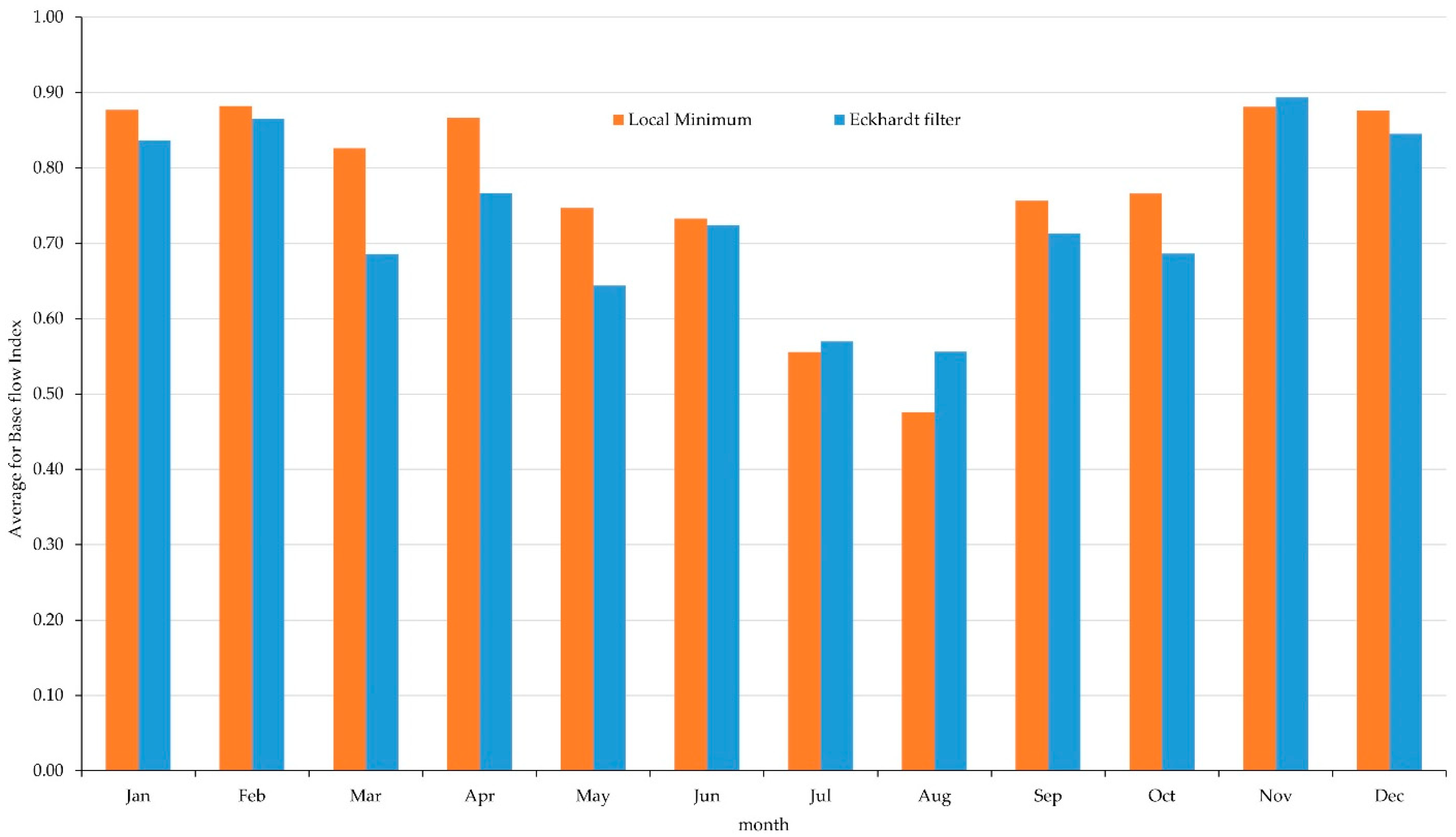
• To compare the two separation methods, namely, the local minimum method (LM) and the Eckhardt filter method (EF), for estimating BF and BFI.
• To evaluate the efficacy of three spatial interpolation approaches (IDW, kriging, and spline) in estimating BF and BFI in ungauged basins.
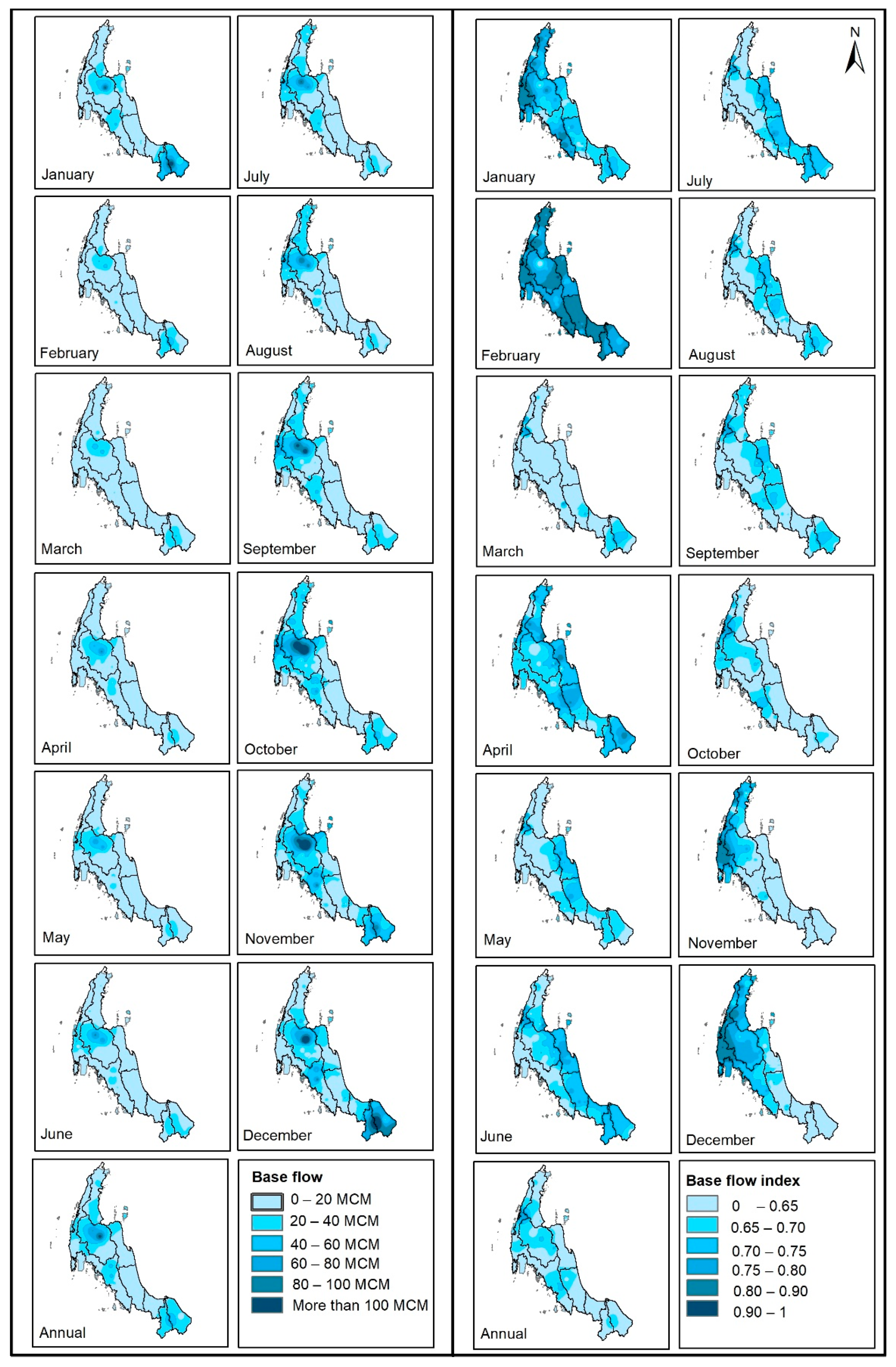
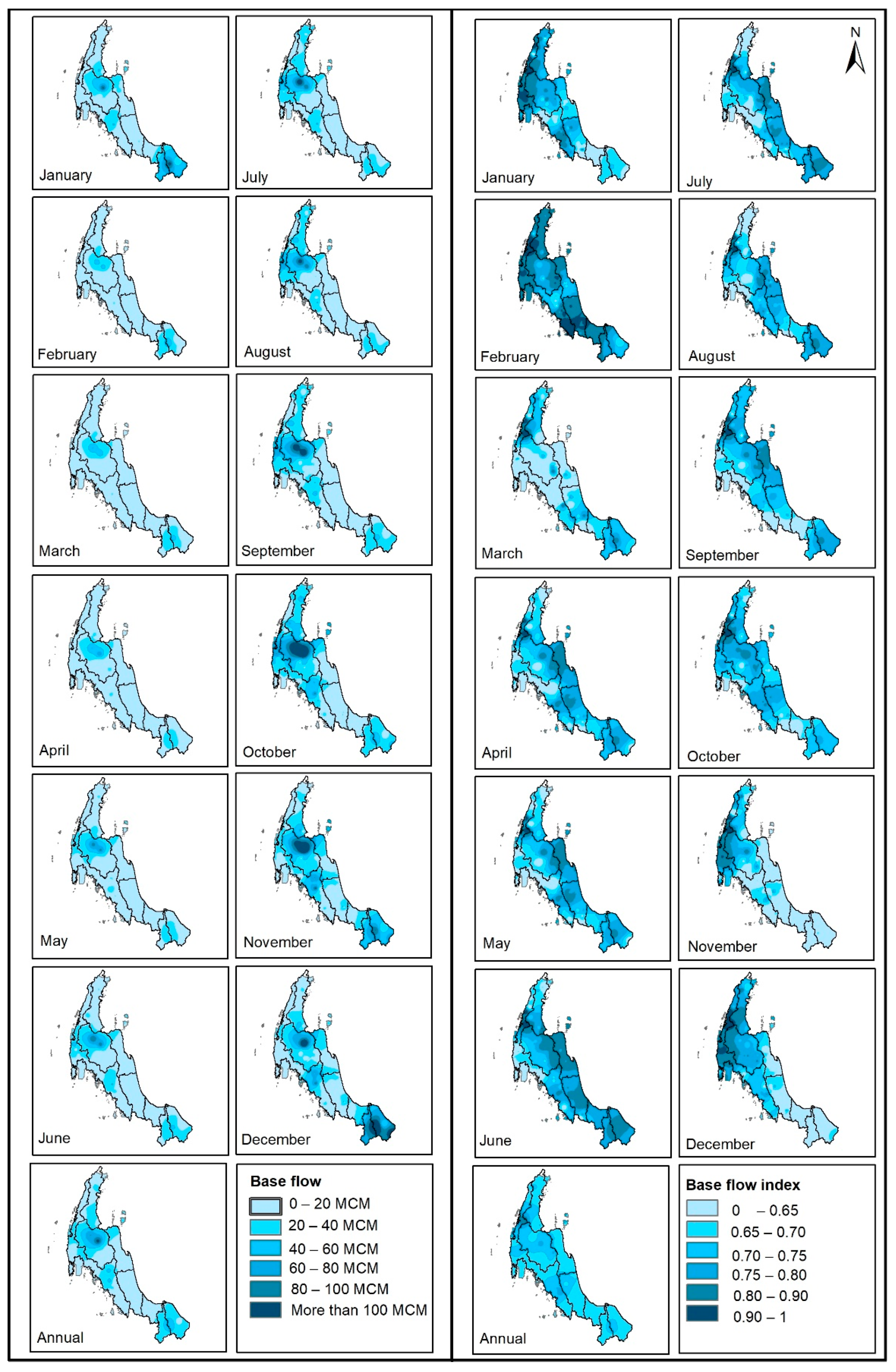
• To create maps showing the BF and BFI’s spatial and temporal variation as useful information for supporting water management-related agencies.

Our investigation results gave more accurate information on the spatial and temporal variation of BF and BFI, which is valuable information for water resource planning and management in our region.

2. Materials and Methods

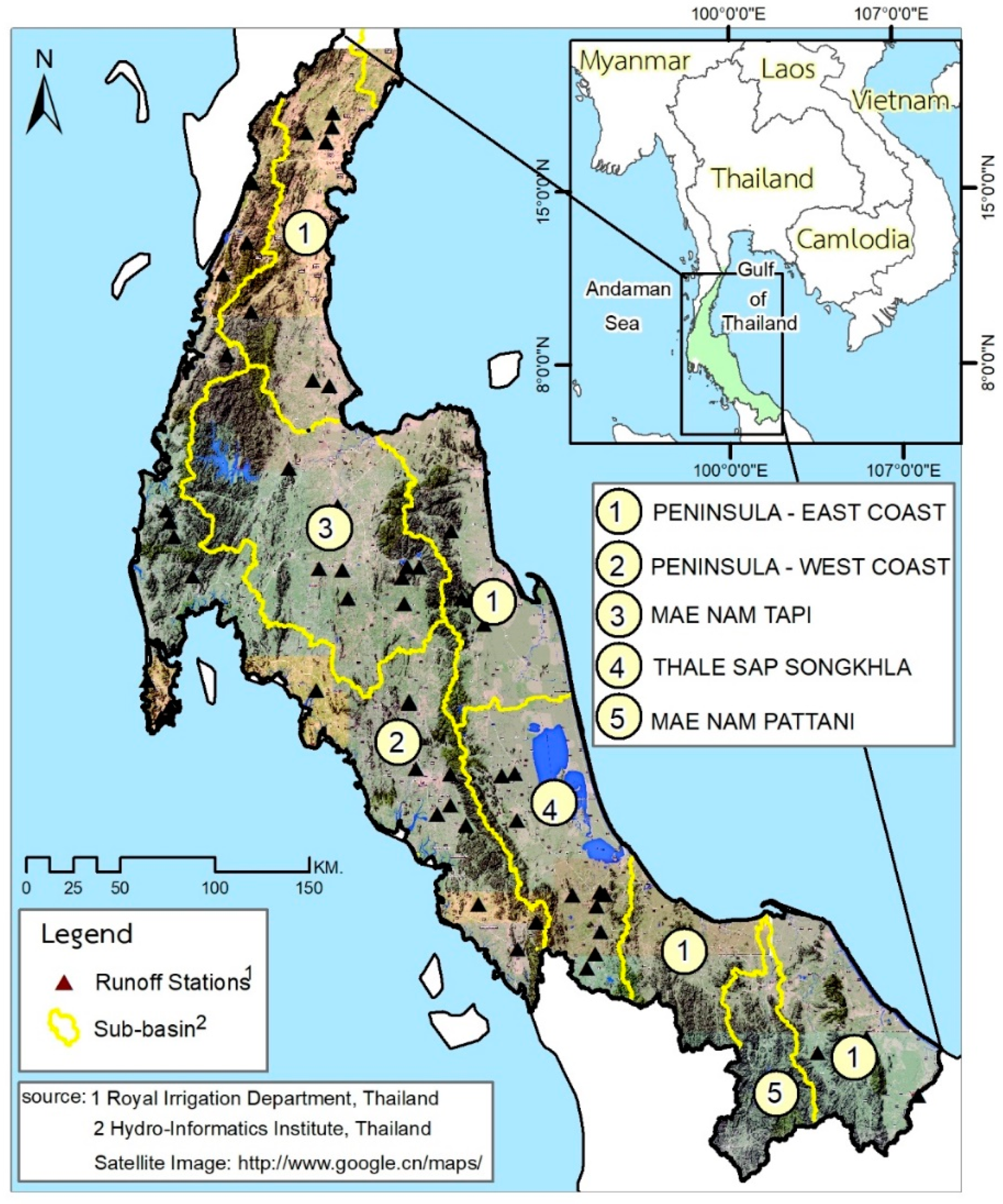
2.1. Study Area and Data Used

Our study focused on the southern river basin of Thailand, which covers five main river basins: the Peninsular-East Coast, the Peninsular-West Coast, Mae Nam Tapi, Thale Sap Songkhla, and Mae Nam Pattani, as depicted in Figure 1. These river basins have areas ranging from 13 to 6713 km² in size. This area is geographically a peninsula between the Andaman Sea’s western side and the South China Sea’s eastern side. It is also extended in the northern and central parts by the long ridge on the west of the mountains. This section is divided into two regions by the Phuket ridge along the west coast and the Nakhon Si Thammarat ridge in the central lower portion of the southern backbone: the east and west coasts. The climate variability on both sides of the river basins was primarily dominated by the northeast monsoon winds and southwest monsoon. The southwestern monsoon wind usually begins in mid-May and ends in mid-October, while the northeastern monsoon typically starts in mid-October and ends in mid-February. The average annual rainfall in this area is approximately 2291 mm, and the average monthly rainfall is between 9 mm and 670 mm. The runoff data used in this analysis were obtained from the daily reports of 65 runoff stations with periods ranging from 4 to 12 years. The annual runoff average is approximately 853 MCM, and the monthly runoff average is between 0.29 MCM and 716 MCM.

Table 1. The meteorological and hydrological characteristics of our studied river basin.

River Basin	Number of Stations	Recorded Period	Area (km2)	Average Rainfall (mm)		Average Runoff (MCM)
				Monthly	Annual	Monthly	Annual
Peninsula-East coast	15	2001–2012	37 to 1504	18 to 619	2249	2 to 710	837
Peninsula-West coast	23	1999–2012	13 to 2798	9 to 2798	2722	0.29 to 416	671
Mae Nam Tapi	10	1999–2012	60 to 6713	22 to 351	1869	5.54 to 716	1657
Thale Sap Songkhla	14	1999–2012	54 to 1849	24 to 613	2033	1 to 242	346
Mae Nam Pattani	3	2001–2012	2361 to 3489	47 to 267	1867	113 to 428	2572
Southern River Basin	65		13 to 6713	9 to 670	2291	0.29 to 716	853

shows the meteorological and hydrological characteristics of the study area.

2.2. Baseflow Separation

In our study, the Web-based Hydrograph Analysis Tool (WHAT) was applied as a method for performing BF separation [32]. It includes one graphical method (local minimum approach) and two digital filter approaches (a digital filter with a one-parameter approach [33] and a digital filter with a two-parameter approach, widely recognized as the Eckhardt filter method). This research applied and compared the results of using the local minimum method and the Eckhardt filter method. Previously, there was research trying to observe the comparison between the Eckhardt filter method and seven other digital filter methods [4]. The description of the local minimum method and the Eckhardt filter method is as follows:

2.2.1. Local Minimum Method (LM)

The LM is one of the graphics approaches used to separate the BF from the total streamflow. Graphics approaches include fixed interval, sliding interval, and local minimum, as introduced by Sloto and Crouse [34]. For each time interval, the LM uses the idea of searching for the two minimum flows and then connecting them with a straight line to separate the BF section from the total runoff. In this regard, the time interval is calculated to determine the lowest discharge within one half the interval minus one day [(2N − 1)/2d] [15] before and after the considered day. The N value is equivalent to A^0.2, where A is the basin area in square miles [35].

2.2.2. Eckhardt Filter Method (EF)

The focus of the EF is on recursive digital filters (RDFs) that apply signal analysis and processing theory to separate the low-frequency signal (BF) from the high-frequency signal (quick flow). There are two parameters, consisting of the filter parameter and BFI_max, for the Eckhardt approach. The filter parameter means the rate at which the streamflow decreases and can be determined directly by a recession analysis after a recharging event. BFI_max is the maximum BFI that a recursive digital filter algorithm can use to create a model. Mathematically, the EF can be expressed as:

$$Q_{b,t}=\frac{\left(1-{\mathrm{BFI}}_{\max }\right)\times \alpha \times Q_{b,t-1}+\left(1-\alpha \right)\times {\mathrm{BFI}}_{\max }\times Q_{s,t}}{1-\alpha \times {\mathrm{BFI}}_{\max }}$$

(1)

where $Q_{b,t}$ and $Q_{b,t-1}$ are the baseflow at step t and t − 1 time, $Q_{s,t}$ is the complete streamflow at step t time; and an is the filter parameter. For the first step in the calculation, the value of $Q_{b,t-1}$ was assumed to be 50% of the total flow as suggested by Zhang, Ahiablame, Engel and Liu [21]. However, empirical judgement would be tried to represent physical reality. Eckhardt [3] recommended representative BFI_max values for three hydrological and hydrogeological conditions: BFI_max = 0.80, for perennial streams with porous aquifers; BFI_max = 0.50, for ephemeral streams with porous aquifers; and BFI_max = 0.25, for perennial streams with hard rock aquifers. The default BFI_max of 0.80 and filter parameters of 0.98 were used in our study, as recommended by WHAT, referring to the hydrological and geological characteristics of the southern river basin of Thailand, a perennial stream of porous aquifers.

2.3. Spatial Interpolation Techniques

2.3.1. Inverse Distance Weighting (IDW)

The inverse distance weighting (IDW) method is based on the principle that locations are closely related to each other, spatially, calculating the value at the desired location where the closest station position will have greater importance. It is an approximation of an unknown point from the linear sum of the known values and the weighted point to be limited by distance. With the distance from the unknown point to the next known point, this weighting is altered and is formulated as follows:

$${\mathrm{Z}}_{\mathrm{i}}=\frac{{\sum }_{\mathrm{i}}\frac{{\mathrm{z}}_{\mathrm{i}}}{{\mathrm{d}}_{\mathrm{ij}}^{\mathrm{n}}}}{{\sum }_{\mathrm{i}}\frac{1}{{\mathrm{d}}_{\mathrm{ij}}^{\mathrm{n}}}}$$

(2)

where Z represents the position of a known point (i) and the predicted value at the unknown point (j), n denotes the exponent that determines the rate of weight reduction as the distance increases (e.g., 1, 2, 3), and d_ij indicates the distance from a known point (i) to an unknown point (j).

2.3.2. Kriging

Kriging proceeds the estimation by giving the weights of the averaged input values. This is similar to the moving-average method for calculating the weight. A semi-variogram model is used to determine the data’s spatial relationship by analyzing the relation between the squared differences of pairs of point values and distance. Therefore, it is necessary to test whether the data are suitable for the model. Kriging is not distance-weighted between the known and unknown positions. Rather, it is the grouping of known positions according to the spatial relationship characteristics that are related to each other and finding the variation to be used as a weight. There are several equations for modulating variograms. Each equation has an initial value of variation (nugget) and the level of the variogram ends. Alternatively, the default constant (sill) and the distance from each point to the sill (range) vary.

The approximation from the variogram was used to estimate the distance-weighted mean when estimating the spatial data. The resulting value is the sum of the known points’ weighted values, depending on the distance between the estimated point and the known point. The weights selected for estimation were not biased. In this study, we herein applied a universal kriging approach. Universal kriging has the form of deterministic interpolation. It hypothesizes that the spatial variation in z values is combined and has spatial relationships with known points. In addition, universal kriging is a method of modulating the area curvature to integrate a plane surface with a quadratic surface, which takes the form of a polynomial equation. It can be described as:

M = b₁x_i + b₂y_i

(3)

$${\mathrm{M}=\mathrm{b}}_1{\mathrm{x}}_{\mathrm{i}}{+\mathrm{b}}_2{\mathrm{y}}_{\mathrm{i}}{+\mathrm{b}}_3{\mathrm{x}}_{\mathrm{i}}^2{+\mathrm{b}}_4{\mathrm{x}}_{\mathrm{i}}{\mathrm{y}}_{\mathrm{i}}{+\mathrm{b}}_5{\mathrm{y}}_{\mathrm{i}}^2$$

(4)

where M is the weight that has a relationship between the point to be approximated and the known point (x_i), y_i is the distance between the points and b₁ and b₂ are the number of pairs of points each by distance h.

2.3.3. Spline

Using a mathematical function to minimize the overall surface curvature, a spline is a deterministic technique used to define two-dimensional curves on three-dimensional surfaces, resulting in a smooth surface that precisely passes through the input points or known points. It can create fairly distinct and visually appealing features using just a few sample points. However, the disadvantages are the resulting surfaces with different minimum and maximum values from the collection of input data. It is prone to outliers, and there is no error sign, which is similar to IDW. For surface interpolation, the algorithm used for the spline utility uses the following formula:

$$\mathrm{S}(\mathrm{x}, \mathrm{y})=\mathrm{T}(\mathrm{x}, \mathrm{y})+{\displaystyle \sum }_{\mathrm{j}=1}^{\mathrm{N}}{\mathsf{\lambda }}_{\mathrm{j}}{\mathrm{R}(\mathrm{r}}_{\mathrm{j}})$$

(5)

where j = 1, 2,..., N; N is the number of points; λ_j are coefficients found by the solution of a linear equation system, and r_j is the distance from point (x, y) to the jth point. T(x, y) and R(r) are defined differently depending on the selected option.

The spline method is a mathematical equation suitable for surfaces with gradual changes, such as the height and depth of the water surface, etc. We chose the regularized spline in this study. A regularized spline is a technique for smoothing the results, where the value of information has a more gradual increase or decrease. The optimal weight value should be between 0–0.5. The regularized spline function is taken as the basis function:

$${\mathrm{T}(\mathrm{x}, \mathrm{y})=\mathrm{a}}_1{+\mathrm{a}}_2{\mathrm{x}+\mathrm{a}}_3\mathrm{y}$$

(6)

where a_i is the coefficient found from the solution of a system of linear equations, and

$$\mathrm{R}\left(\mathrm{r}\right)=\frac{1}{2\mathsf{\pi }}\{\frac{{\mathrm{r}}^2}{4}\left[\ln \left(\frac{\mathrm{r}}{2\mathsf{\tau }}\right)+\mathrm{C}-1\right]{+\mathsf{\tau }}^2{[\mathrm{K}}_0\left(\frac{\mathrm{r}}{\mathsf{\tau }}\right)+\mathrm{C}+\ln \left(\frac{\mathrm{r}}{2\mathsf{\pi }}\right)]\}$$

(7)

where r is the distance between the point and the sample, τ² is the weight parameter, K₀ is the modified Bessel function and “C” is a constant equal to 0.577215.

3. Results and Discussion

The present study deals with estimating BF and BFI in ungauged basins in the southern river basin of Thailand. Three major results, as indicated in our research objective, are presented and discussed as follows: (1) comparative results of estimating BF and BFI using two separation methods (i.e., LM and EF methods); (2) evaluation of the efficacy of three spatial interpolation approaches (i.e., IDW, kriging, and spline) in estimating BF and BFI in ungauged basins; and (3) maps showing the spatial and temporal variations of BF and BFI. The details are presented as follows:

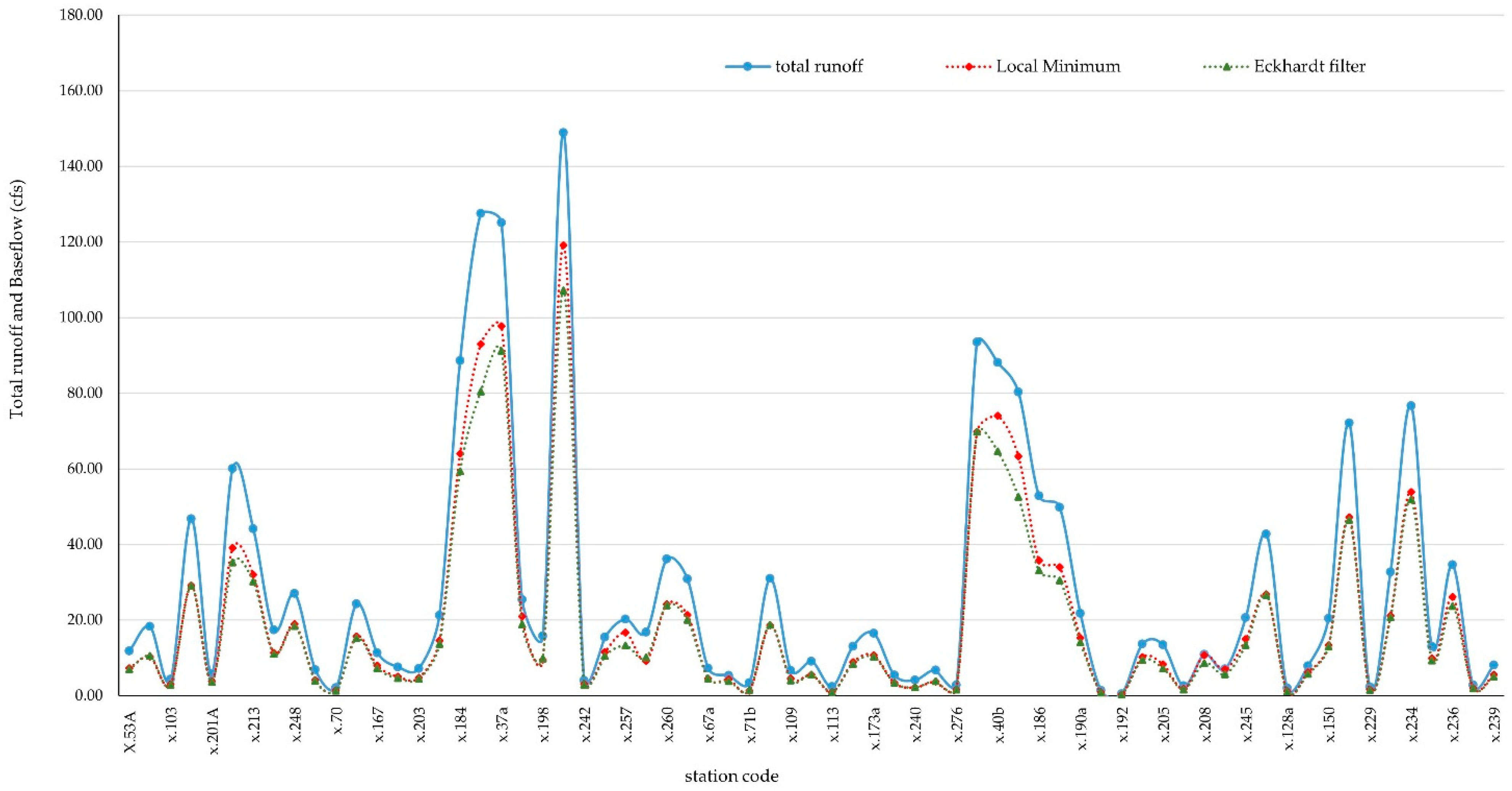
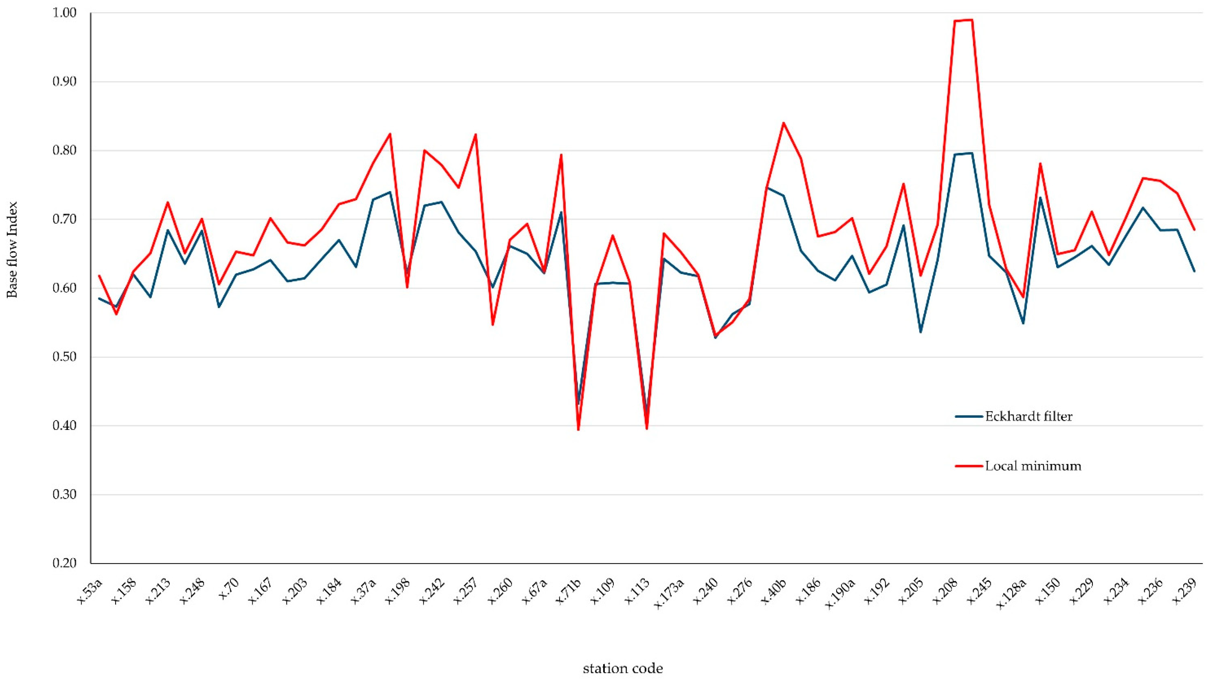
3.1. Local Minimum Method vs. Eckhardt Filter Method for Estimating BF and BFI

The spatial variation of the annual runoff and BF performed by the LM and EF methods for the 65 runoff stations is shown in Figure 2. The BF computed by the LM method had a bit higher value than that calculated by the EF method. Additionally, Figure 3 shows the BFI for 65 runoff stations calculated using the LM and EF methods. We generally found the same trend as the BF; that is, the BFI calculated by the LM method had a higher value than that calculated by the EF method. It is because LM’s determination process of the lowest discharge to separate baseflow from total runoff gives the local minimums and depends on the calculated time interval as a function of the basin area. Additionally, the baseflow values for each day between local minimums are estimated by linear interpolations. Therefore, it may result in overestimation in BF and BFI. On the other hand, the EF considers the shorter interval (day by day in this experiment), obtaining the smoother and more refined baseflow values.

Figure 4 and Figure 5 show an example of the temporal variation of the total runoff, BF, and BFI at the X.248 runoff station. We observed that almost every month of the year, BF, and BFI were given by LM had higher values than those provided by EF, except in July, August, and November. During these three months, X.248 runoff station is influenced by the southwest monsoon wind (July and August) and the northeast monsoon wind (November), resulting in a high runoff. As explained previously, the EF method gives smoother and more refined baseflow values than those provided by the LM method. As a result, the LM method may produce underestimation in BF and BFI since the baseflow values for each day between local minimums are estimated by linear interpolations.

Using two statistical indices (namely, mean difference (MD) and correlation coefficient (r)), a distinction was made between these two annual and monthly BF and BFI methods, as shown in

Table 2. Comparison of BF and BFI values for all 65 runoff stations calculated by EF and LM.

BF (MCM)

Indices

Jan

Feb

Mar

Apr

May

Jun

Jul

Aug

Sep

Oct

Nov

Dec

Annual

MD

−0.16

−0.20

−1.27

0.06

−1.89

−1.94

−1.56

−1.56

−2.36

−4.31

−1.68

−0.45

−1.45

r

0.993

0.993

0.990

0.956

0.997

0.999

0.994

0.992

0.997

0.998

0.997

0.997

0.998

BFI

Indices

Jan

Feb

Mar

Apr

May

Jun

Jul

Aug

Sep

Oct

Nov

Dec

Annual

MD

−0.01

−0.02

−0.08

−0.06

−0.08

−0.07

−0.06

−0.07

−0.06

−0.09

−0.03

−0.01

−0.04

r

0.883

0.770

0.797

0.795

0.848

0.885

0.837

0.852

0.886

0.865

0.896

0.924

0.926

. This indicates that the BF and BFI, as computed by the EF method, had lower values than those values as computed by the LM method for both annual and monthly periods. The results are similar compared to those found by Schilling and Jones [7]. It can be noted from the acquisition of MD’s negative values that the discrepancy between the values given by EF and those given by LM, except for the BF result in April, gave a positive value (0.06 MCM) that was an inverse meaning, as discussed previously. In October, the maximum difference in value of the BF and BFI was −4.31 MCM and −0.09, respectively. In addition, there was a very high correlation between the two approaches, i.e., r ≥ 0.95 for BF and r ≥ 0.70 for BFI.

3.2. Performance Comparison of Spatial Interpolation Techniques

To investigate the performance of three spatial interpolation techniques (namely, IDW, kriging, and spline), we randomly selected our data sets three times with 75% and 25% of the total 65 runoff stations for the calibration and validation stages, respectively. Thus, we had three different repeated samples for each considered period, i.e., April representing a dry season, November representing a monsoon season, and annual, for BF and BFI. Using two separation methods, i.e., LM and EF, we finally had a total of 36 study cases (3 cases by randomly selecting three times from the whole data sets, 3 cases from three considered periods, 2 cases by having BF and BFI, and 2 cases for two baseflow separation methods) in our experiment. The information in Table 2 and

Table 3. Comparison of the statistical indices for spatial interpolation techniques in estimating BF.

BF
Methods	r			MAE			RMSE			CA			Stage	Period
	I	K	S	I	K	S	I	K	S	I	K	S
LM	1.00	0.34	0.99	0.01	8.54	0.76	0.04	12.38	1.48	0.02	7.19	0.75	Calibration	April
EF	1.00	0.37	0.99	0.01	7.91	0.76	0.04	11.03	1.49	0.02	6.53	0.75
LM	0.65	0.38	0.20	9.26	12.78	23.53	15.51	18.55	39.13	8.36	10.61	20.96	Validation
EF	0.66	0.39	0.31	10.02	12.41	22.88	16.55	19.24	35.96	8.95	10.71	19.69
LM	1.00	0.37	1.00	0.16	23.08	0.19	0.04	32.08	0.32	0.06	18.47	0.17	Calibration	November
EF	1.00	0.44	1.00	0.01	20.29	0.25	0.03	27.44	0.45	0.02	15.98	0.23
LM	0.56	0.31	0.34	21.86	23.51	42.59	39.51	42.01	71.15	20.47	21.91	37.81	Validation
EF	0.53	0.27	0.34	21.04	22.80	40.38	35.73	38.35	67.15	18.96	20.48	35.76
LM	1.00	0.52	1.00	0.00	12.59	0.05	0.00	18.48	0.08	0.00	10.50	0.04	Calibration	Annual
EF	1.00	0.61	1.00	0.00	10.75	0.04	0.00	14.99	0.07	0.00	8.70	0.04
LM	0.61	0.54	0.37	11.27	12.26	20.22	19.03	20.20	27.49	10.19	10.95	16.03	Validation
EF	0.61	0.53	0.39	10.77	11.09	18.43	17.55	18.06	24.81	9.54	9.85	14.54

Remark: I = IDW; K = kriging; and S = spline.

shows a summary of the comparative statistical metrics, that is, mean absolute error (MAE), root mean squared error (RMSE), correlation coefficient (r), and combined accuracy (CA) for the three spatial interpolation techniques in estimating BF and BFI. These were the average values from three randomly selected times, as mentioned above. The higher performance of interpolation technique gives the lower MAE and RMSE, and r approaching 1.0 [36]. The combined accuracy (CA) [37] refers to the combination of RMSE, MAE, and r², which equals 0.33 *(RMSE + MAE + (1 − r²)) and should be as small as possible (optimally 0).

Table 3 and

Table 4. Comparison of the statistical indices for spatial interpolation techniques in estimating BFI.

BFI
Methods	r			MAE			RMSE			CA			Stage	Duration
	I	K	S	I	K	S	I	K	S	I	K	S
LM	1.00	0.52	1.00	0.00	0.12	0.00	0.00	0.16	0.00	0.00	0.33	0.00	Calibration	April
EF	1.00	0.51	1.00	0.00	0.10	0.00	0.00	0.13	0.00	0.00	0.31	0.00
LM	0.81	0.59	0.55	0.10	0.13	0.15	0.12	0.17	0.26	0.18	0.31	0.35	Validation
EF	0.31	0.06	0.20	0.07	0.07	0.12	0.09	0.09	0.17	0.33	0.38	0.40
LM	1.00	0.72	1.00	0.00	0.08	0.00	0.00	0.10	0.00	0.00	0.22	0.00	Calibration	November
EF	1.00	0.86	1.00	0.00	0.05	0.00	0.00	0.07	0.10	0.00	0.13	0.03
LM	0.50	0.54	0.20	0.11	0.10	0.18	0.14	0.13	0.24	0.33	0.30	0.44	Validation
EF	0.67	0.68	0.36	0.08	0.08	0.13	0.10	0.10	0.19	0.24	0.23	0.37
LM	1.00	0.46	1.00	0.00	0.06	0.00	0.00	0.08	0.00	0.00	0.30	0.00	Calibration	Annual
EF	1.00	0.52	1.00	0.00	0.04	0.00	0.00	0.06	0.00	0.00	0.27	0.00
LM	0.40	0.25	0.19	0.07	0.07	0.12	0.10	0.10	0.19	0.33	0.35	0.41	Validation
EF	0.25	0.18	0.07	0.05	0.05	0.09	0.07	0.07	0.12	0.34	0.34	0.39

Remark: I = IDW; K = kriging; and S = spline.

show comparisons of the statistical indices for spatial interpolation techniques in estimating BF and BFI, respectively. The findings revealed that among the three spatial interpolation techniques, IDW gave the best performance. It provided the highest r-value and the lowest values of MAE, RMSE, and CA for both the calibration and validation stages. We can notice the bold number showing the best values of r, MAE, RMSE, and CA in Table 3 and Table 4. Most of these indices pointed out IDW as giving the best performance, followed by kriging and spline, respectively. It was similar to the results found by Ly, Charles and Degré [28] for estimating monthly rainfall data. We further noticed that the use of the IDW and spline techniques overfitted in our data sets because the values of r, MAE, RMSE, and CA for the calibration stage were significantly different from those values in the validation stages. In contrast, the kriging technique gave less difference in the values between the two stages. We found that the kriging technique gave a lower r-value and higher MAE, RMSE, and CA values than the values provided by the spline technique for the calibration stage. However, it also mostly gave higher r-values and lower MAE, RMSE, and CA values than those given by the spline technique for the validation stage. It indicated that overfitting occurred for Spline technique for estimating BF and BFI in this experiment. This made the kriging technique more suitable or generalized than the spline technique for estimating BF and BFI in our study region. The reason why the computed BF by the LM and EF methods in the dry season for the validation stage gave better results (higher r-value, lower MAE, RMSE, and CA values) because less runoff fluctuation and less amount of runoff were noticed in the dry season for all runoff stations resulting in the data range was narrower as compared to those in the monsoon season. The data range in April used for the validation stage for the LM method was narrower than that for the EF method. As a result, the LM method’s r, MAE, RMSE, and CA values were better than the EF method’s. The data range in November used for the validation stage for the EF method was narrower than that for the LM method. As a result, the EK method’s r, MAE, RMSE, and CA values were better than the LM method’s.

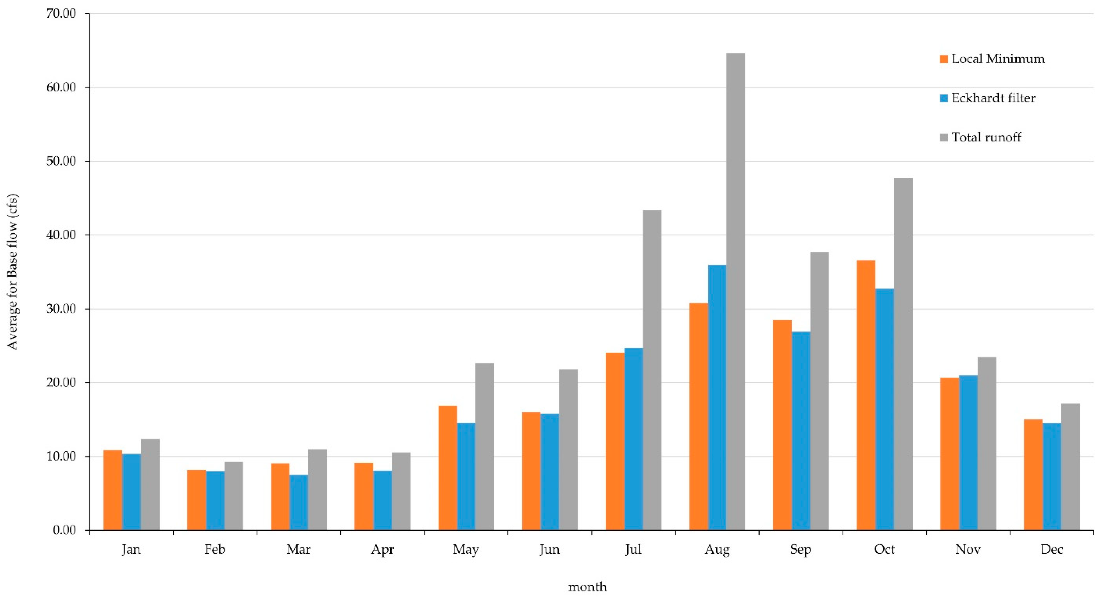
3.3. Spatio-Temporal Variation of BF and BFI Using IDW Method

As the IDW method was the best spatial interpolation technique for our study, it was used to create the spatio-temporal variation of monthly and annual BF and BFI maps with a resolution of 30 × 30 m². Figure 6 and Figure 7 show the monthly and annual BF and BFI, calculated by the EF and LM methods, respectively. We can explain and discuss the following: the maximum average annual BF was found at the Mae Nam Tapi river basin, where the BF value varied in the range of 80 MCM to more than 100 MCM, followed by the Mae Nam Pattani river basin and the upper part of the Peninsular-West Coast river basin, where the BF value varied in the range of 80 MCM to 100 MCM. The minimum average annual BF was found in the Thale Sap Songkhla river basin, where the BF value was lower than 20 MCM. For the average annual BFI, we found that the maximum value ranging from 0.75 to 0.80 was located at the upper part of the Peninsular-West Coast River basin, followed by the Mae Nam Tapi river basin and the lower part of the Peninsular-West Coast river basin, where the BFI value varied in the range of 0.70 to 0.75. The minimum average annual BFI was found in the lower part of the Peninsular-East Coast river basin, where the BFI value was lower than 0.65. Considering the monthly BF, we found that the maximum BF value occurred between October and January, which is during the monsoon season. In addition, we found the Mae Nam Tapi river basin gave the maximum BF value during October and November, whereas the Mae Nam Pattani river basin gave the maximum BF value ranging from 80 MCM to more than 100 MCM. As naturally found in the dry season, the minimum BF value occurred between February and June, and most of the southern river basins had this values lower than 20 MCM. For the monthly BFI, the maximum BFI value happened in February, from the end of the monsoon season to the beginning of the dry season, for most of the southern river basin, where the BFI value varied in the range of 0.90 to 1.0. For the other months, we clearly found a difference in the high value of the BFI between the Peninsular-East Coast and Peninsular-West Coast areas because of the effect of the northeast monsoon and southwest monsoon winds, respectively. During April and September, a high value of BFI ranging between 0.70 and 0.90 was found in the Peninsular-East Coast area, that is, the Peninsular-East Coast, Mae Nam Tapi, Thale Sap Songkhla, and Mae Nam Pattani river basins. However, during October and January September, a high value of BFI ranging between 0.70 and 0.90 was found in the Peninsular-West Coast river basin. We also found that the minimum BFI value of less than 0.70 happened in March, which is in the dry season, for most of the southern river basins.

4. Conclusions

In this study, we mainly aimed to estimate the monthly and annual BF and BFI. Three spatial interpolation approaches (i.e., IDW, kriging, and spline) were applied to assess their efficacy. In addition, we compared two baseflow separation methods (namely, the LM and EF methods) for estimating BF and BFI. Our study area included 65 runoff gauged stations located in the southern river basins of Thailand. The findings revealed that the BF and BFI, calculated using the EF method, had lower values than those calculated using the LM method for both annual and monthly periods. More than 75% of the basins in the southern part of Thailand had a BFI of more than 0.60, indicating quite considerable water source potential in this region. For our experiment, IDW provided the best performance among the three interpolation techniques, followed by kriging and spline, respectively. Finally, monthly and annual BF and BFI maps with a resolution of 30 × 30 m² were created in this research work. They provide valuable information for water management agencies in regard to planning and managing water resources in the southern river basin of Thailand.

References

1. Meyer, S.C. Analysis of base flow trends in urban streams, northeastern Illinois, USA. Hydrogeol. J. 2004, 13, 871–885. [Google Scholar] [CrossRef]
2. Sophocleous, M. Interactions between groundwater and surface water: The state of the science. Hydrogeol. J. 2002, 10, 52–67. [Google Scholar] [CrossRef]
3. Eckhardt, K. How to construct recursive digital filters for baseflow separation. Hydrol. Process. 2005, 19, 507–515. [Google Scholar] [CrossRef]
4. Eckhardt, K. A comparison of baseflow indices, which were calculated with seven different baseflow separation methods. J. Hydrol. 2008, 352, 168–173. [Google Scholar] [CrossRef]
5. Shao, G.; Zhang, D.; Guan, Y.; Sadat, M.A.; Huang, F. Application of different separation methods to investigate the baseflow characteristics of a Semi-Arid Sandy Area, Northwestern China. Water 2020, 12, 434. [Google Scholar] [CrossRef] [Green Version]
6. Gonzales, A.L.; Nonner, J.; Heijkers, J.; Uhlenbrook, S. Comparison of different base flow separation methods in a lowland catchment. Hydrol. Earth Syst. Sci. 2009, 13, 2055–2068. [Google Scholar] [CrossRef] [Green Version]
7. Schilling, K.E.; Jones, C.S. Hydrograph separation of subsurface tile discharge. Environ. Monit. Assess. 2019, 191, 231. [Google Scholar] [CrossRef] [PubMed]
8. Đukić, V. Modelling of base flow of the basin of Kolubara river in Serbia. J. Hydrol. 2006, 327, 1–12. [Google Scholar] [CrossRef]
9. Cartwright, I.; Gilfedder, B.; Hofmann, H. Contrasts between estimates of baseflow help discern multiple sources of water contributing to rivers. Hydrol. Earth Syst. Sci. 2014, 18, 15–30. [Google Scholar] [CrossRef] [Green Version]
10. Chen, H.; Teegavarapu, R.S.V. Comparative analysis of four baseflow separation methods in the south Atlantic-gulf region of the U.S. Water 2019, 12, 120. [Google Scholar] [CrossRef] [Green Version]
11. Minea, I. Streamflow-base flow ratio in a lowland area of North-Eastern Romania. Water Resour. 2017, 44, 579–585. [Google Scholar] [CrossRef]
12. Ibrahim, B.; Wisser, D.; Barry, B.; Fowe, T.; Aduna, A. Hydrological predictions for small ungauged watersheds in the Sudanian zone of the Volta basin in West Africa. J. Hydrol. Reg. Stud. 2015, 4, 386–397. [Google Scholar] [CrossRef] [Green Version]
13. Lacey, G.C.; Grayson, R.B. Relating baseflow to catchment properties in south-eastern Australia. J. Hydrol. 1998, 204, 231–250. [Google Scholar] [CrossRef]
14. Haberlandt, U.; Klöcking, B.; Krysanova, V.; Becker, A. Regionalisation of the base flow index from dynamically simulated flow components—A case study in the Elbe River Basin. J. Hydrol. 2001, 248, 35–53. [Google Scholar] [CrossRef]
15. Mazvimavi, D.; Meijerink, A.M.J.; Savenije, H.H.G.; Stein, A. Prediction of flow characteristics using multiple regression and neural networks: A case study in Zimbabwe. Phys. Chem. Earth 2005, 30, 639–647. [Google Scholar] [CrossRef]
16. Gebert, W.A.; Radloff, M.J.; Considine, E.J.; Kennedy, J.L. Use of streamflow data to estimate base flow/ground-water recharge for Wisconsin. J. Am. Water Resour. Assoc. 2007, 43, 220–236. [Google Scholar] [CrossRef]
17. Neff, B.P.; Day, S.M.; Piggott, A.R.; Fuller, L.M. Base Flow in the Great Lakes Basin (No 2005-5217); US Geological Suvey: Reston, VA, USA, 2005. [CrossRef]
18. Longobardi, A.; Villani, P. Baseflow index regionalization analysis in a mediterranean area and data scarcity context: Role of the catchment permeability index. J. Hydrol. 2008, 355, 63–75. [Google Scholar] [CrossRef]
19. Bloomfield, J.P.; Allen, D.J.; Griffiths, K.J. Examining geological controls on baseflow index (BFI) using regression analysis: An illustration from the Thames Basin, UK. J. Hydrol. 2009, 373, 164–176. [Google Scholar] [CrossRef] [Green Version]
20. Zhu, Y.; Day, R.L. Regression modeling of streamflow, baseflow, and runoff using geographic information systems. J. Environ. Manag. 2009, 90, 946–953. [Google Scholar] [CrossRef]
21. Zhang, Y.; Ahiablame, L.; Engel, B.; Liu, J. Regression modeling of baseflow and baseflow index for Michigan USA. Water 2013, 5, 1797–1815. [Google Scholar] [CrossRef] [Green Version]
22. Ahiablame, L.; Chaubey, I.; Engel, B.; Cherkauer, K.; Merwade, V. Estimation of annual baseflow at ungauged sites in Indiana USA. J. Hydrol. 2013, 476, 13–27. [Google Scholar] [CrossRef]
23. Hong, M.; Zhang, R.; Wang, D.; Qian, L.; Hu, Z. Spatial interpolation of annual runoff in ungauged basins based on the improved information diffusion model using a genetic algorithm. Discret. Dyn. Nat. Soc. 2017, 2017, 1–18. [Google Scholar] [CrossRef]
24. Priestley, C.H.B.; Taylor, R.J. On the assessment of surface heat flux and evaporation using large-scale parameters. Mon. Weather Rev. 1972, 100, 81–92. [Google Scholar] [CrossRef]
25. Shyamala, G.; Arun Kumar, B.; Manvitha, S.; Vinay Raj, T. Assessment of spatial interpolation techniques on groundwater contamination. In Proceedings of the International Conference on Emerging Trends in Engineering (ICETE), Hyderabad, India, 22–23 March 2019; Springer: Cham, Switzerland, 2020; pp. 262–269. [Google Scholar] [CrossRef]
26. Yan, T.; Zhao, W.; Zhu, Q.; Xu, F.; Gao, Z. Spatial distribution characteristics of the soil thickness on different land use types in the Yimeng Mountain Area, China. Alex. Eng. J. 2021, 60, 511–520. [Google Scholar] [CrossRef]
27. Meng, Q.; Liu, Z.; Borders, B.E. Assessment of regression kriging for spatial interpolation—Comparisons of seven GIS interpolation methods. Cartogr. Geogr. Inf. Sci. 2013, 40, 28–39. [Google Scholar] [CrossRef]
28. Ly, S.; Charles, C.; Degré, A. Different methods for spatial interpolation of rainfall data for operational hydrology and hydrological modeling at watershed scale: A review. Biotechnol. Agron. Société Et Environ. 2013, 17, 392–406. [Google Scholar]
29. Li, J.; Heap, A.D. Spatial interpolation methods applied in the environmental sciences: A review. Environ. Model. Softw. 2014, 53, 173–189. [Google Scholar] [CrossRef]
30. Eva, Y.-H.; Wu, M.C.H. Comparison of spatial interpolation techniques using visualization and quantitative assessment. In Applications of Spatial Statistics; InTech: Rijeka, Croatia, 2016. [Google Scholar] [CrossRef] [Green Version]
31. Santhi, C.; Allen, P.M.; Muttiah, R.S.; Arnold, J.G.; Tuppad, P. Regional estimation of base flow for the conterminous United States by hydrologic landscape regions. J. Hydrol. 2008, 351, 139–153. [Google Scholar] [CrossRef]
32. Lim, K.J.; Engel, B.A.; Tang, Z.; Choi, J.; Kim, K.S.; Muthukrishnan, S.; Tripathy, D. Automated web GIS based hydrograph analysis tool, WHAT. J. Am. Water Resour. Assoc. (JAWRA) 2005, 41, 1407–1416. [Google Scholar] [CrossRef]
33. Lyne, V.; Hollick, M. Stochastic time-variable rainfall-runoff modelling. In Proceedings of the Institute of Engineers Australia National Conference, Perth, WA, Australia, 10–12 September 1979; pp. 89–93. [Google Scholar]
34. Sloto, R.A.; Crouse, M.Y. HYSEP: A computer program for streamflow hydrograph separation and analysis. Water Resour. Investig. Rep. 1996, 96, 4040. [Google Scholar] [CrossRef]
35. Linsley, R.K.J.; Kohler, M.A.; Paulhus, J.L. Hydrology for Engineers; McGraw-Hill: New York, NY, USA, 1982. [Google Scholar]
36. Achu, A.L.; Thomas, J.; Aju, C.D.; Gopinath, G.; Kumar, S.; Reghunath, R. Machine-learning modelling of fire susceptibility in a forest-agriculture mosaic landscape of southern India. Ecol. Inform. 2021, 64, 101348. [Google Scholar] [CrossRef]
37. Eray, O.; Mert, C.; Kisi, O. Comparison of multi-gene genetic programming and dynamic evolving neural-fuzzy inference system in modeling pan evaporation. Hydrol. Res. 2017, 49, 1221–1233. [Google Scholar] [CrossRef]
Figure 1. Locations of selected runoff stations in the southern river basin, Thailand.
Water 13 03113 g001
Figure 2. Spatial variation of annual runoff and BF for 65 runoff gauged stations.
Water 13 03113 g002
Figure 3. Spatial variation of annual BFI for 65 runoff gauged stations.
Water 13 03113 g003
Figure 4. Temporal variation of total runoff and BF at X.248 runoff gauged station.
Water 13 03113 g004
Figure 5. Temporal variation of total BFI at X.248 runoff gauged station.
Water 13 03113 g005
Figure 6. Spatio-temporal variation of BF and BFI by using the EF method.
Water 13 03113 g006
Figure 7. Spatio-temporal variation of BF and BFI by using the LM method.
Water 13 03113 g007