
A Fuzzy Logic Model for Early Warning of Algal Blooms in a Tidal-Influenced River

National Key Laboratory of Water Environmental Simulation and Pollution Control, Guangdong Key Laboratory of Water and Air Pollution Control, South China Institute of Environmental Sciences, Ministry of Ecology and Environment, No. 18 Ruihe Road, Guangzhou 510530, China
*
Author to whom correspondence should be addressed.
Water 2021, 13(21), 3118; https://doi.org/10.3390/w13213118
Submission received: 30 July 2021
/
Revised: 12 October 2021
/
Accepted: 18 October 2021
/
Published: 5 November 2021
(This article belongs to the Special Issue Ecosystem-Based Understanding and Management of Eutrophication)
Abstract
:Algal blooms are one of the most serious threats to water resources, and their early detection remains a challenge in eutrophication management worldwide. In recent years, with more widely available real-time auto-monitoring data and the advancement of computational capabilities, fuzzy logic has become a robust tool to establish early warning systems. In this study, a framework for an early warning system was constructed, aiming to accurately predict algae blooms in a river containing several water conservation areas and in which the operation of two tidal sluices has altered the tidal currents. Statistical analysis of sampled data was first conducted and suggested the utilization of dissolved oxygen, velocity, ammonia nitrogen, total phosphorus, and water temperature as inputs into the fuzzy logic model. The fuzzy logic model, which was driven by biochemical data sampled by two auto-monitoring sites and numerically simulated velocity, successfully reproduced algae bloom events over the past several years (i.e., 2011, 2012, 2013, 2017, and 2019). Considering the demands of management, several key parameters, such as onset threshold and prolongation time and subsequent threshold, were additionally applied in the warning system, which achieved a critical success index and positive hit rate values of 0.5 and 0.9, respectively. The differences in the early warning index between the two auto-monitoring sites were further illustrated in terms of tidal influence, sluice operation, and the influence of the contaminated water mass that returned from downstream during flood tides. It is highlighted that for typical tidal rivers in urban areas of South China with sufficient nutrient supply and warm temperature, dissolved oxygen and velocity are key factors for driving early warning systems. The study also suggests that some additional common pollutants should be sampled and utilized for further analysis of water mass extents and data quality control of auto-monitoring sampling.
1. Introduction
As urban, industrial, and agricultural activities rapidly increase, their attendant environmental issues have also intensified to the great concern of scientists and the public. Algal blooms are one such issue and have become a serious threat to water resources worldwide [1,2]. Algae blooms induce problems such as depletion of oxygen [3], decreased biodiversity [4,5], and reduced water transparency. These problems pose serious risks to human health [6], fisheries, and [7] water resource sustainability. For example, in water conservation areas [8], waterworks must stop operating when algae blooms occur. Preventing severe deterioration of water quality due to the fact of this issue will require effective environmental management techniques. Of particular importance are early warning techniques aimed at identifying algae blooms before or as they occur [9]. This enables rapid response by the aquaculture industry and other stakeholders at the onset of algae blooms and increases the chance of mitigating their impacts.
In recent years, a wide variety of predictive methods have been developed to forecast algae blooms [10]. They aim to provide an estimation of the likelihood of occurrence and abundance over short or long timescales [11]. Mechanistic models typically describe the growth, transport, and decline of phytoplankton [12]. The complexity of these approaches varies with considered mechanisms, the data availability, and the requirement of prediction. Statistical models rely on large data sets and tend to be tailored to the specific data set used for their development. However, theoretical frameworks, such as mechanisms and expert knowledge, may be difficult to implement in a purely data-driven statistical model.
Furthermore, the precision of the aforementioned methods is constrained by many factors. First, the definition of a ‘bloom’ event varies among algal species and the requirements of management. Some species form a visible bloom or have a significant impact even with a concentration below a certain density (e.g., Dinophysis spp. can be harmful at <103 cells L−1 [13]). Second, the crucial drivers and processes of algal blooms are still not fully understood. The high degree of spatiotemporal heterogeneity in species composition, food–web interactions, and forms and fluxes of nutrients all account for the imperfect performance of forecasts [14]. Third, notable public events of algae blooms underscore the gaps between scientific knowledge and applied management [15]. The closure of drinking water facilities in Toledo, Ohio, in 2014 points to the vulnerable linkages between public demands and scientific research, which has persisted for two decades, indicating that focusing on the nutrient concentration is not sufficient for prevention and detection of bloom events [16]. In particular, for coastal areas, shore-based and off-shore monitoring were suggested to be implemented together to provide sufficient information for decision making regarding beach closures and aquaculture management practices during blooms [17], even though the high financial costs often hinder the execution.
New statistical techniques have been deployed to predict algal blooms in response to observations. Combined with new mechanistic models, statistical data-driven models enable a deeper understanding of the processes governing the initiation, growth, transport, and decline of algae, which leads to significant improvements in predicting blooms [18]. A fuzzy logic model is a typical example of a data-based empirical–statistical model integrated with known processes. Fuzzy logic is a modeling approach [19] with the ability to reflect human behavior, which enables it to deal with uncertain and ambiguous subjects [20] such as currency exchange rates [21], weather prediction [22], and risk assessment [23]. In environmental science, fuzzy logic is widely used to develop environmental indices, especially with respect to water quality. Instead of assigning a single qualification to a state variable (e.g., a temperature of 20 °C is ‘high’), fuzzy logic applies the concept of memberships of multiple qualifications. For instance, a temperature of 20 °C is assigned a membership of 0.75 for the qualification ‘intermediate’ and a membership of 0.25 for the qualification ‘high’. In this way, the degree to which quantitative inputs are assigned to each category determines the membership. This allows for a more continuous representation of the state variables. Second, using IF-THEN rules to embody a premise or known causality, fuzzy logic can combine knowledge of the processes affecting algae blooms with the conceptual criteria of environmental management. To illustrate, IF the temperature is high, the current velocity is low and the nutrient concentration is high, THEN the probability of a bloom is high. With the advantage in considering known processes and utilizing real-time observation together, fuzzy logic shows promise as an effective tool for building forecasting systems for algal blooms [24,25].
The Shawan River (Figure 1), located at the center of the Guangdong–Hong Kong–Macau Greater Bay Area, serves as an important drinking water source. However, it has connections with other tidal channels (the Shiqiao River) that receive domestic and industrial sewage. Furthermore, the bidirectional tidal currents decrease the exchange efficiency of water mass, which increases the vulnerability of the water quality of the Shiqiao River. There have been two recorded algae blooms: from 25 October to 25 December 2010 and from 22 to 28 October 2012. To prevent further severe deterioration of drinking water resources due to the fact of algae blooms, sampling of relevant biochemical factors and construction of an early warning system were carried out in 2013 and 2014. Subsequently, this study aimed to develop an early warning index of algae blooms based on a fuzzy logic model. Section 2 provides a brief introduction of the study area and the framework of the early warning system. Section 3 presents the application and evaluation of the established model. Section 4 contains an analysis of the sensitivity of the framework with respect to the model structure and the setting of thresholds. Section 5 provides the conclusion and future outlooks.
2. Materials and Methods
2.1. Study Site
The Pearl River Delta (PRD) is a complex large-scale estuarine system in the south of China that consists of many tidal river network branches. The Shawan–Shiqiao basin (Figure 1), with a total area of 229.8 km2, is located in the central PRD in Panyu District of Guangzhou City. This area is quite shallow, with a depth in most parts of less than 10 m (Figure 1). Stratifications are rarely found in this area. It is surrounded by the Shawan and Shiqiao rivers, which are influenced by irregular semidiurnal tides and upstream runoff. The Shawan River meets the type II water quality standards of China (GB3838-2002: dissolved oxygen (DO) ≥ 6 mg/L, chemical oxygen demand (CODCr) ≤ 15 mg/L, ammonia nitrogen (NH3-N) ≤ 0.5 mg/L, and total phosphorous (TP) ≤ 0.1 mg/L) and neighbors several water conservation areas (Figure 1). It is the designated Drinking Water Protected River of Panyu District, providing drinking water for thousands of people. In contrast, the Shiqiao River receives large amounts of domestic sewage and agricultural non-point source. It is subsequently heavily polluted and only meets the type IV water quality requirements (DO ≥ 3 mg/L, CODCr ≤ 30 mg/L, NH3-N ≤ 1.5 mg/L, and TP ≤ 0.3 mg/L).
As parts of the tidal river network of the Pearl River, the Shiqiao River and the Shawan River experience flood and ebb currents twice per day. Driven by the bidirectional flow, water is interchanged between the two rivers, which enhances the spread of polluted water from the Shiqiao River [26]. The bidirectional flow also hinders the outflow of polluted water and prolongs the residence time of pollutants, which further deteriorates the environmental conditions.
To promote the water quality of the Drinking Water Source Conservation Area in the Shawan River, the tide sluices located in Yanzhou and Longwan were constructed and began service in 2010. The Yanzhou Sluice only opens during the ebb tidal phase, whereas the Longwan Sluice only opens at the flood tidal phase. This has essentially changed the flow pattern from bidirectional to unidirectional. The salty water from downstream floods into the Shawan River and the polluted water mass in the Shiqiao River is drained downstream during the ebb tidal phase, which largely prevents the spread of pollution into the Shawan River. The combined dispatching of the two sluices speeds up the water exchange, increases the water environmental capacity, and improves the water’s self-purification ability, which helps to restore the ecological environment of the river systems.
2.2. Post-Algae Bloom Sampling and Selection of Input Variables
There were two recorded algae bloom events in the Shawan River from 25 November 2012 to 8 December 2012 and from 22 to 28 October 2012. On 24 October 2012, the cell abundance reached 1.04 × 10⁷ ind/L and the chlorophyll-a concentration was 69.5 µg/L. To detect the water quality conditions of algal growth, three field samplings were conducted in the Shiqiao and Shawan rivers on 22 November 2013, 24 October 2014, and 21 November 2014. Five sampling sites (i.e., S1, S2, S4, S5, and S7) were chosen on the main channel of the Shawan River, and two sampling sites were assigned to the two tributary inflow points (i.e., S3, S6). To better capture the potential influence of the Yanzhou Sluice and downstream channels, two additional sites were chosen along the Shiqiao River. S9 was placed near the river fork of the DJL, the only connection between the two rivers, and S10 was set to capture the downstream influences. The 18 variables sampled were water temperature (Tem), atmospheric temperature, pH, velocity (Vel) of river flow, suspended matter, transparency, DO, DO saturation rate, NH3-N, nitrate, nitrite, total phosphorous (TP), dissolved inorganic phosphate (DIP), silicate (SiO4), potassium permanganate index (CODMn), chlorinity (Cl), dissolved inorganic nitrogen (DIN), and chlorophyll-a (Chl-a).
The collected data revealed the basic conditions and the variation in ranges of the hydrodynamic and biochemical factors in this area. In the three sampling periods, the velocity of the Shawan River ranged from 0.010 m/s to 0.310 m/s. The average velocities for 22 November 2013, 24 October 2014, and 21 November 2014 were 0.152 m/s, 0.146 m/s, and 0.099m/s, respectively. Salinity varied only slightly, ranging from 0.01 to 0.13 among all the samplings. Under adequate nutrient conditions, the optimum value of the ratio N:P:Si for algae growth is 16:1:15 (Redfield–5 Brzezinski ratio) [27,28]. The minimum threshold concentrations for algae growth are 0.152 mg/L for Si, 0.035 mg/L for DIN, and 0.01 mg/L for DIP [29]. Across the three sampling periods, the ratio of SiO4:DIP ranged from 53 to 260, that of SiO4:DIP ranged from 2 to 4, and that of DIN:DIP ranged from 18 to 91, which indicates that phosphate was the most important limiting nutrient and that the concentration of Si was sufficient for the growth of diatoms. In the first two sampling periods, the dominating algae were diatoms, whereas Cryptomonas spp. were dominant during the third period. However, only in the third campaign did the density of algae cells meet the threshold of an algae bloom (1.04 × 10⁶ ind/L).
To select suitable variables as inputs for the fuzzy logic model, all sampled variables were analyzed by principal component analysis (PCA) [30] and canonical correspondence analysis (CCA) [31]. In the PCA, the first two components that contributed the most variance were extracted and further analyzed. The corresponding variables of the top four weighting coefficients of each PCA component and the ranking of sites with the four highest relative coefficients are all listed in Table 1. NH3-N and TP were important variables with high weighting coefficients in PCA1, particularly at S10 and S9, which indicates the severe nutrient pollution in the Shiqiao River. In contrast, the Shawan River was characterized by high COD with a negative weighting coefficient of DO, indicating that the organic pollutants were more salient and that the self-purification driven by algae growth was thriving. Velocity was also an important variable in the top two PCAs in all three sampling periods, particularly in the downstream section (S10, S9, S8, S7) and upper stream (S1, S2) of the Shawan River.
A CCA analysis was also conducted to extract the environmental factors that influence the distribution of algae species. Prior to the CCA, correlation analysis was used to confirm the independence of these environmental variables. Algae species with relative abundances higher than 1% were selected. The results of CCA indicated that the CODMn, DO, DIN, DIP, and temperature were important factors that influenced the distribution of algae species. Diatoms were relatively insensitive to organic pollutants, DO, and nutrients, which indicates that diatoms may maintain high abundances for longer periods. In contrast, Cryptomonas species were more sensitive to nutrient availability. However, green algae displayed an opposite variation trend toward the concentration of organic pollutants and were not recorded as a dominant species in the Shawan River.
The analysis revealed that the DO, NH3-N, TP, Vel, and Tem were the most relative variables to agal blooms and should drive the early warning model. Two auto-monitoring stations (Figure 1) are located at Shawan River. The first station, Panyu station (PY), is located on the left side of the upper stream of the Shawan River. The other, Dongchong station (DC), is on the right side of the downstream section. The monitoring stations measured 11 parameters every two hours including Tem, pH, DO, conductivity, NH3-N, TP, CODMn, cyanide, hexavalent chromium [Cr (VI)], copper, and cadmium. The time series sampled by the two monitoring stations ranged from 2011 to 2012 and 2017–2019. Considering that DO values change dramatically between day and night when algae blooms occur, we used the maximum daytime (7:00 to 19:00) DO concentration minus the minimum nighttime value (19:00 to 7:00) as an input for the early warning model. This value was denoted by ΔDO. Because velocity was not automatically monitored by the PY and DC stations, it was supplemented by a validated numerical simulation.
2.3. Numerical Simulation
To obtain the simulated velocity for the fuzzy logic model, a 3D hydrodynamical–biochemical numerical model, the Environmental Fluid Dynamics Code (EFDC) [32], was applied to the Shawan–Shiqiao basin. The EFDC was developed by John Hamrick at Virginia Institute of Marine Science. It includes modules such as hydrodynamics, sediment, toxic substances, sediment, waves, and water quality [33]. It has been applied worldwide in various surface water systems such as rivers, lakes, estuaries, wetlands, and coastal regions [34]. The model solves the vertically hydrostatic, free-surface, turbulent averaged equations of motion for a variable-density fluid, using second-order accurate, spatial finite differences on a staggered C-grid. To include the influence of the sluice operation on the velocity field, temporal variations were added using the ‘mask.inp’ function in the EFDC model. In this instance, the EFDC model was able to imitate the opening and closing of the sluice by mandating ‘mask.inp’ to play the ‘blocking’ role at appointed time steps [35]. The code version 7.1 of EFDC was applied in this study. The simulation of the Shawan–Shiqiao basin was formulated on orthogonal curve coordinate grids, with a spatial resolution ranging from 100 to 300 m. In total, it had 273 × 97 simulation cells in the horizontal direction, with 1 layer in the vertical direction since the deepest bathymetry was no more than 10 m. The horizontal resolution ranged from 3.6 to 11.0 m. The time step was 1 s, and the output time step was 20 min, which allowed for a robust representation of processes of physics and biogeochemistry. The simulation was forced with meteorological conditions. Pollutants loading from upstream channels were interpolated from seasonal observations and operation data of sewage treatment plants near the Shiqiao River. Hydrodynamical boundary conditions were provided by a validated simulation covering the whole Pearl River Estuary domain [36], of which the river flow was interpolated from the daily-averaged value sampled by the Bureau of Hydrology and Water Resources of Pearl River, and water elevations at the lower boundary were originally driven by the Global Tide Assimilation Data [37]. The operations of the two tide gates were implemented based on the records of sluice operations in reality. The full simulation period encompassed 59 days, which was initialized on 1 January 2014 and ended on 28 February 2014, with a spin-up time period for 10 days.
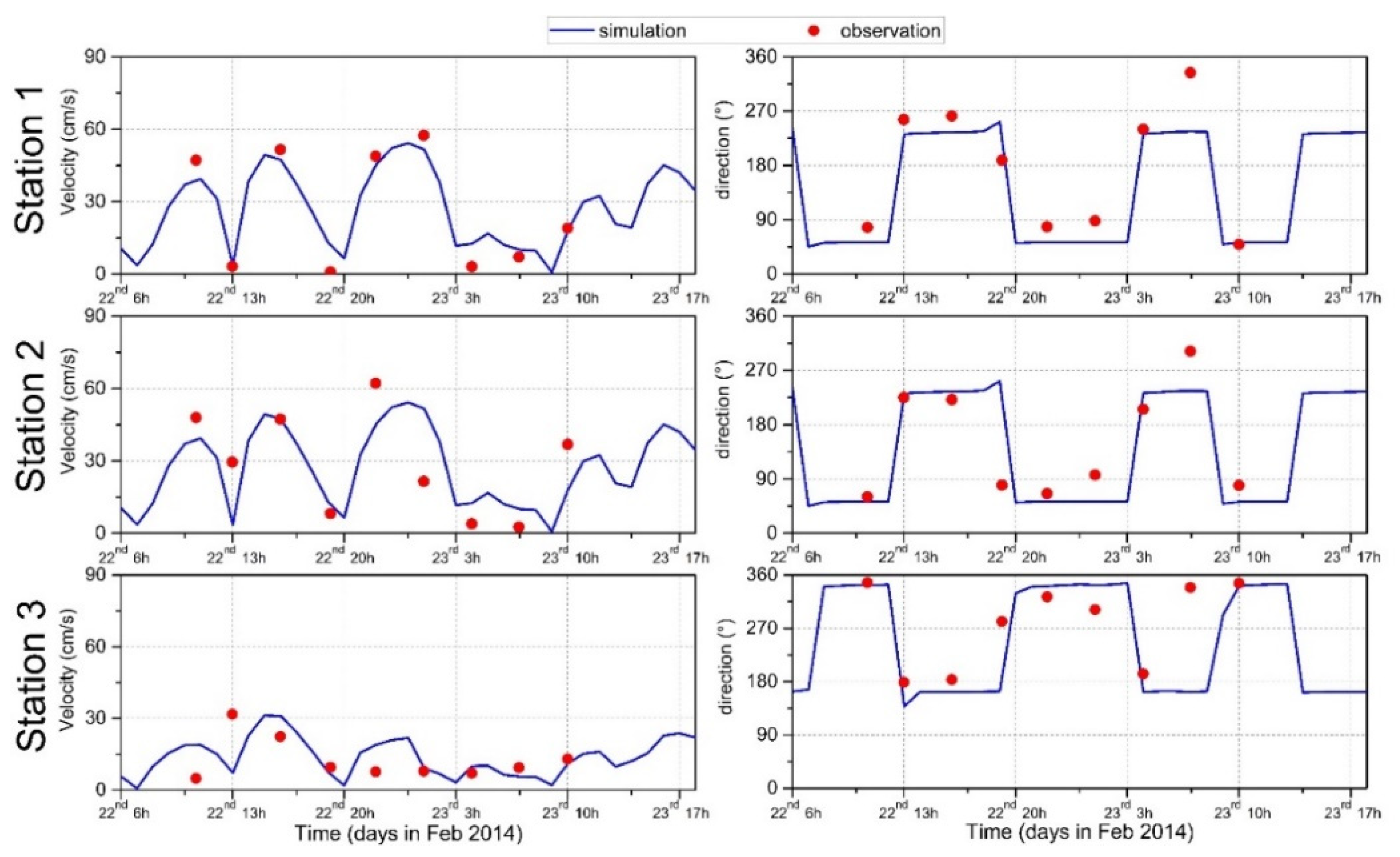
To validate the performance of the EFDC simulation, velocity time series sampled at three sites on 22–23 February 2014 were compared with the simulated values (Figure 2). The simulation successfully captured the major variations in velocity induced by sluice operation and tides. The absolute discrepancy between the speeds was less than 8.8 cm/s. In 92.3% of the time steps, the inaccuracy of direction was less than 60°.
2.4. Development of an Early Warning Index Based on Fuzzy Logic
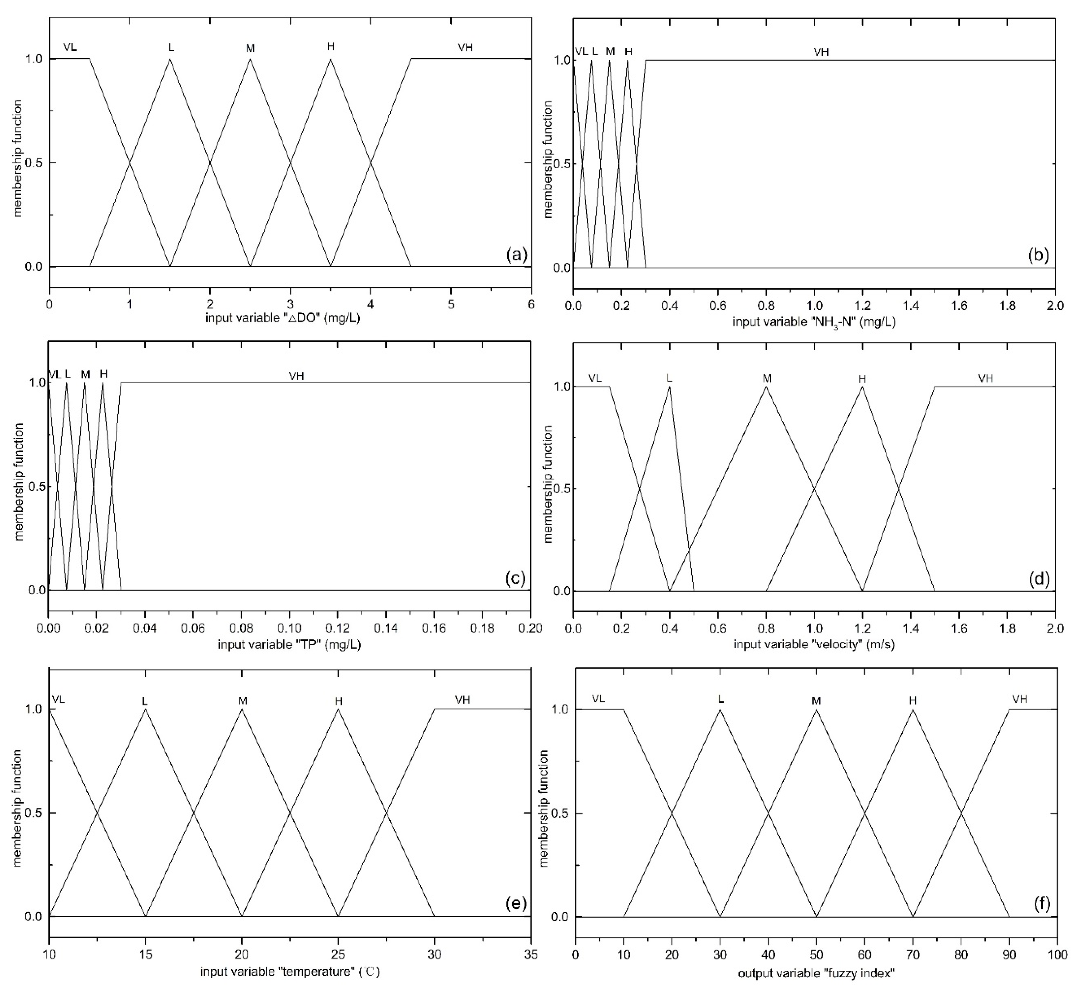
The design and structure of the fuzzy logic model is shown in Figure 3. The inputs of the model are shown in the left column including biogeochemical data and hydrologic data such as temperature from auto-monitoring measurements and flow velocity from the EFDC simulation. In the first step, all input data went through fuzzification. NH3-N, TP, ΔDO, Vel, and Tem were translated into memberships of sets of qualitative descriptions (Figure 4). The second step, called fuzzy inference, including fuzzy rules and fuzzy operators, are shown in the middle column. The fuzzy rules, which embody the IF-THEN logical chain, were designed based on knowledge of processes. In this study, three water quality variables were first converted into a water quality index (WQI) by fuzzy rules. Then, the influence of the WQI and physical variables were merged to generate the fuzzy sets of early warning variables. In the defuzzification step, the fuzzy sets of early warning variables were translated into a numerical output that quantitatively described the probability of algae bloom occurrence. Considering the temporal resolution of the data sets, the warning system provides early warning indexes every day. The results on day T + 1 only relies on the conditions on T. Once the early warning index exceeds thresholds, measures are taken on time to safeguard the operation of the water works.
2.4.1. Fuzzification
The fuzzification process consists of the definition of the fuzzy sets and membership functions. In the first step, input values for all variables are converted into several fuzzy sets, with membership grades determining the extent to which a value belongs to a fuzzy set. This is based on a defined fuzzy logic, which is a mechanism for describing the degree of membership of an element to a set and the use of several terms to classify the linguistic variables.
The traditional mathematics of logical judgements is based on binary logic, which is also referred to as the law of bivalence. The law of bivalence responses are ‘completely true’ and ‘completely false’. For example, it may classify a water temperature value greater than 30 °C as ‘hot’, whereas a value even slightly less than 30 °C is ‘not hot’. Zadeh [19] introduced fuzzy logic to extend the law of bivalence. Fuzzy logic introduces the concept of partial truth-values that lie between ‘completely true’ and ‘completely false’. This aligns with patterns of human thinking, which generally do not determine such categories in a precise sense, necessitating a transition between ‘not hot’ and ‘hot’ (Figure 4). Figure 4e illustrates two fuzzy logic concepts, ‘fuzzy sets’ and ‘membership functions’. In this example, ‘hot’ is defined as a linguistic term corresponding to a fuzzy subset of ‘H’ of the variable ‘water temperature’. The membership function in Figure 4e numerically represents the degree to which an element belongs to ‘H’.
A membership function describes all information contained in a fuzzy set. Fuzzy set theory permits the gradual assessment of the membership of elements in relation to a set. In theory, the fuzzy set ‘A’ is a subset of a non-empty space X, and can be defined as:
where x1 belongs to X and is an element of fuzzy set A, and the value of μA(x) shows the membership grade of x1 in fuzzy set A. μA(x1) = 1 signifies full membership of element x1 to fuzzy set A, μA(x1) = 0 means that no element of x1 belongs to fuzzy set A, and 0 < μA(x1) < 1 indicates partial membership of element x1 to fuzzy set A.
A membership function can be expressed in various forms such as triangular, trapezoidal, and Gaussian [38]. In this study, the triangular and trapezoidal membership functions were combined to characterize the transitions between different fuzzy sets (Figure 4). The ranges of these five parameters were identified by finding the minimum and maximum values of each parameter. Five fuzzy sets were defined by the linguistic terms, named as very low (VL), low (L), medium (M), high (H), and very high (VH). Each set was divided based on a literature review and local climate and hydrological characteristics, which are listed in Table 2. Each input variable was assigned a membership function that ranged from 0 to 1 on the defined linguistic terms.
2.4.2. Fuzzy Inference
Fuzzy inference consists of fuzzy rules and fuzzy operators. In the fuzzy rules, knowledge of processes is laid down in a set of ‘IF-THEN’ rules to describe the relationship between the input and output fuzzy sets. For example, IF the water temperature is ‘high’ AND the flow velocity is ‘very low’, THEN the probability of an algal bloom is ‘very high’. The principle of the rule block WQI is that the lowest of these three variables determines the WQI [45]. Generally, a high ΔDO value indicates that an algal bloom may occur, as phytoplankton produce oxygen during the day and consume it at night. A high concentration of NH3-N or TP indicates that there are sufficient nutrients to support phytoplankton growth. Considering that the depletion of nutrients (NH3-N and TP) could limit phytoplankton growth or a low ΔDO value could indicate a poor growth state, the lowest of the three values is supposed to limit the probability of a bloom. Hence, if ‘ΔDO’ is ‘M’, ‘NH3-N’ is ‘H’, and ‘TP’ is ‘L’, then the lowest of these three parameters is ‘L’; thus, ‘WQI’ is ‘L’.
The fuzzy sets of physical variables (i.e., Tem, Vel) and the WQI were inputs of the rule block ‘Early warning index’. The growth rate of phytoplankton generally increased with Tem [46]. However, it typically decreased when Tem exceeded 30 °C, representing a physiological temperature limit [42]. Only when Tem was ‘H’ instead of ‘VH’ was an algal bloom highly likely to occur.
The inference rules for the rule block ‘Early warning index’ are more complicated than that of WQI and, subsequently, the details are provided in Table 3. Fuzzy set operations determine the process to combine the results from each fuzzy rule. The union operation creates a new subset from two or more input subsets by uniting them as defined by the following equation [47]:
2.4.3. Defuzzification
In the final step, the linguistic outputs of fuzzy inference are translated into a quantitative but relative value for each time step, indicating the degree to which surface blooms may appear. The center of gravity (COG) method was applied in the defuzzification. Its discrete form is based on Equation (3), in which μ(xi) is the membership value for point xi [47]:
2.5. Assessment Routine of Hindcast Results
To better define the beginning and end of the warning period based on the output of the fuzzy logic model, we developed a method to determine the time when the warnings of algae blooms tend to initiate and terminate. It consists of an onset threshold that indicates the issuing of the bloom, a subsequent threshold by which whether the warning should extend, and a proper prolongation time which determines how long the warning should be extended. To find an appropriate prolongation time for the alarm after the warning index time series exceeds the onset threshold, potential values for the prolongation time ranging 1–15 days were compared with the bloom periods in the records. After reaching the onset threshold, the warning index series was tested with an interval of 10 in the range of 10 to 60 to find an appropriate value for a subsequent threshold. If the warning index series following the initial threshold reaches the defined subsequent threshold, the warning should be extended for the defined prolongation time. The results of the various prolongation times and subsequent thresholds were evaluated by 3 typical criteria: the critical success index (CSI) [48], true positive hit rate (TPR), and false alarm rate (FAR) [49]. The equations are listed below:
TNP is the number of positive cases in which the alarm is raised. TN is the number of negative cases (no bloom) in which the alarm is not raised. FP is the number of false alarms raised in the absence of a bloom. FN is the number of times when blooms occurs, but no alarm is raised. Based on the above-mentioned equations, the CSI is proportional to the frequency of the event being forecast, and The TPR quantifies the percentage of TRUE events among all alarming events. The higher the CSI and TPR, the more reliable the forecasting system. On the contrary, the FAR is the percentage shared by false alarms among all alarming events. Values of the 3 statistical criteria range from 0 to 1. When the values of CSI and TPR approach 1, the robustness of the system is verified and vice versa for FAR.
3. Results
3.1. Hindcast of the Recorded Algae Blooms
Two algae blooms were recorded in the Shawan River during 2011–2012 according to the available data. These occurred from 25 November to 8 December 2011 and from 22 to 28 October 2012. Both blooms began on the southern side of the Shawan River and spread to the northern side, fully covering the Water Resource Protected Areas during the bloom peak.
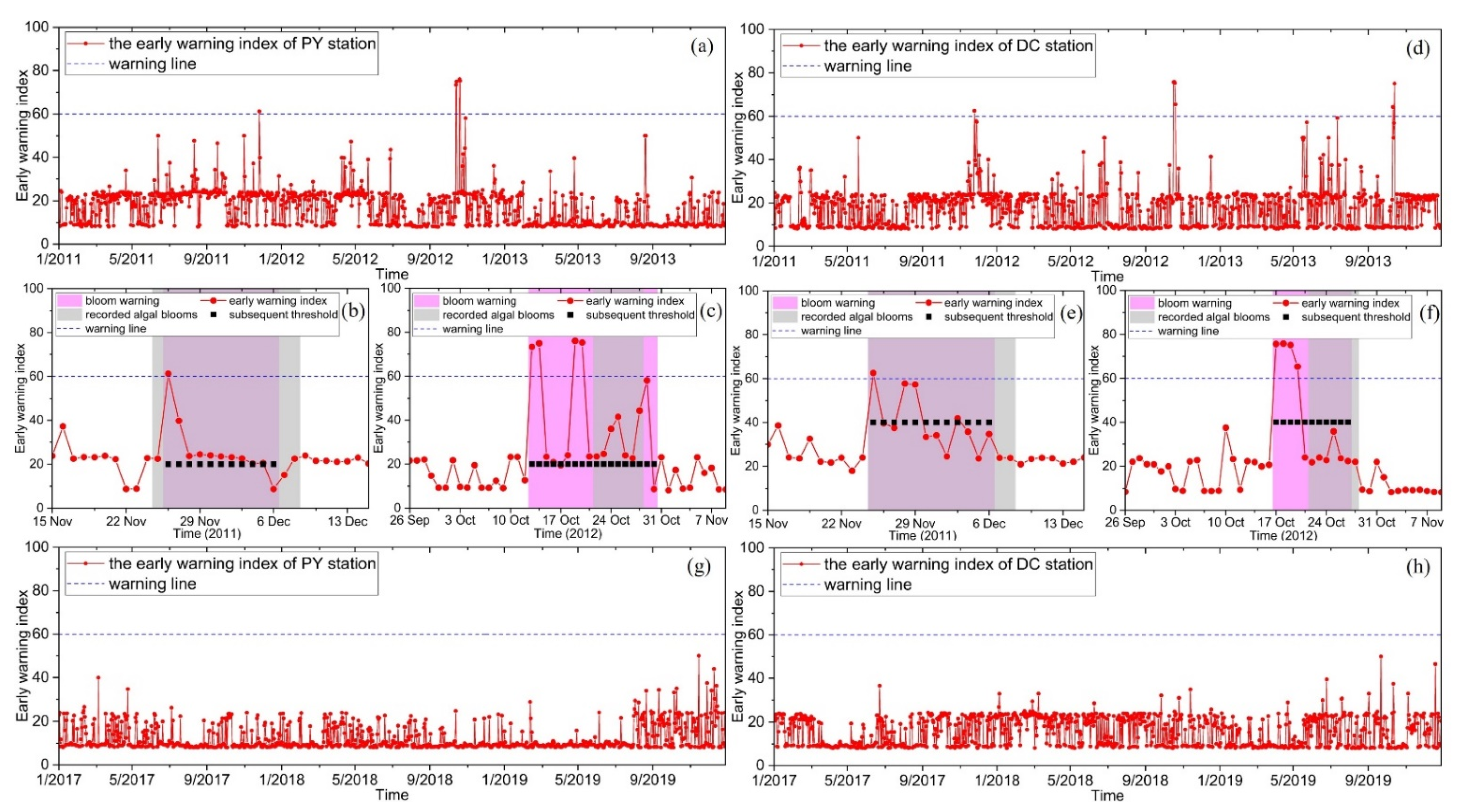
Figure 5 illustrates the daily values of the early warning index based on fuzzy logic for the PY and DC stations. High values of the early warning index indicate a high probability of an algal bloom. By comparing the warning index and the records of visible blooms, the index value of 60 was assigned as the onset threshold for the occurrence of an algae bloom (Figure 5). The value of the warning index over the 2 year sampling generally remained below 60 with the exception of two periods (Figure 5a,d). On 26 November (Figure 5b), the day after the records of a visible algal bloom, the early warning index reached 62 (>60). On 13 October 2012 (Figure 5c), the early warning index also rose above 60 and successfully predicted an algal bloom that began on 22 October 2012. In accordance with the hindcast result of the PY station, the early warning index of the DC station reached 62 (>60) on 26 November 2011 (Figure 5e), which was exactly when a visual bloom was recorded. The early warning index also reached 75.67 on 17 of October 2012, which was 5 days prior to the recorded algae bloom (Figure 5f). During 11–14 of October 2013, the warning index maintained a high value ranging from 50 to 75 in the DC station; however, no blooms were recorded during this period at the PY station. The fuzzy logic model was also run for the period of 2017 to 2019, for which auto-monitoring data were available. Consistent with the absence of algae blooms during this period, the warning index remained below 60, demonstrating the robustness of the fuzzy logic warning model.
3.2. Statistical Assessment of the Results
The early warning index resulting from the fuzzy logic model is difficult to evaluate using standard assessments. Firstly, exceeding the defined threshold of the warning index only indicates the probable occurrence of an algal bloom, which is challenging to compare directly with the record of blooms. In particular, information on the onset of blooms is lacking as the rapid duplication of phytoplankton cells probably begins several days prior to the first record of a visible bloom. However, in observations of this study, the bloom was only recorded when the density of algal cells reached a salient level. Highlighting the importance of early warning, it is often too late to sound the alarm when blooms have already reached a severe stage and the water quality can no longer serve its designed functions in the water conservation areas. Lastly, sounding the alarm based on a spiky early warning index and a single threshold for the onset of blooms cannot predict the duration of algal blooms. If sufficient nutrient concentrations or ΔDO sustain, the index could maintain a relatively high value, which may indicate continued growth or favorable growing conditions for algae. For this reason, the prolongation time and subsequent threshold were introduced to additionally predict the time at which the blooms were expected to disappear.
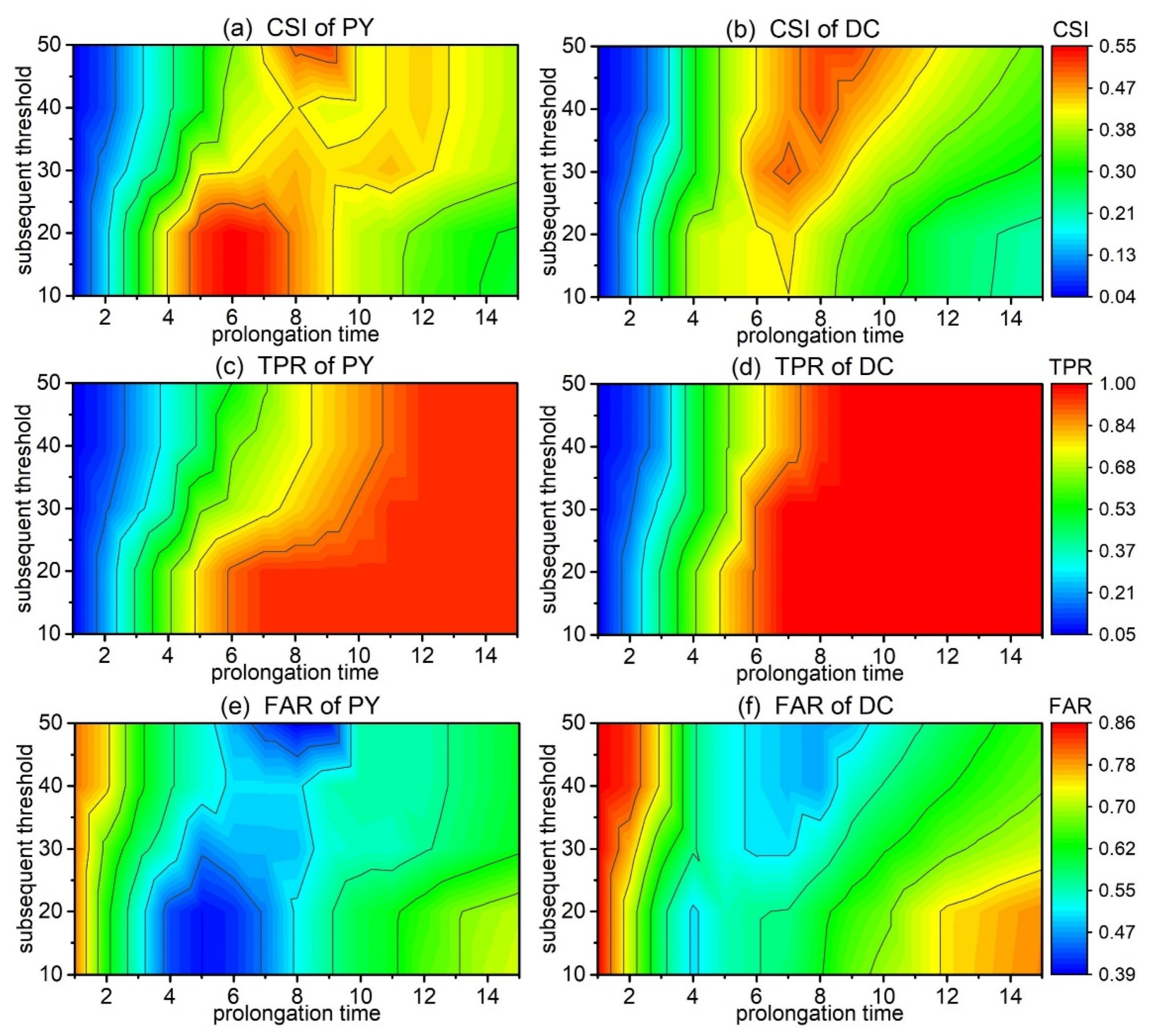
The values of CSI, TPR, and FAR are plotted in Figure 6 as functions of the prolongation time of the alarm and the subsequent threshold. For both the DC and PY stations, the CSI first increased with the prolongation time, reached a peak after 6–8 days, and then decreased (Figure 6a,b). This indicates that the typical duration of algal blooms in this area was 6–8 days. The longer the alarm was sounded, the fewer days during the bloom were likely to be missed, which is why the TPR generally increased with the prolongation time (Figure 6c,d). When the prolongation time reached 11 days, the TPR approached 1, which suggested that this represents the upper limit of the duration of visible bloom events in this area. In the range of a prolongation time from 6 to 8 days, the TPR at the PY station decreased when warning index values less than 30 were not counted (Figure 6c). In other words, subsequent thresholds higher than 30 were too high for the PY station and caused the station to omit bloom periods that occurred. However, the TPR of the DC station was not sensitive to the variations in thresholds (Figure 6d). As seen in the enlarged time series in Figure 5e,f, we found that lower subsequent thresholds were more suitable for the PY station (Figure 5b,c), probably due to the systematic difference between the two stations. Following the major peak above 60, the warning index of PY tended to decrease rapidly (Figure 5b,c), even if the bloom was present according to the records. Increasing the subsequent thresholds shortened the duration of the alarm and, thus, increased the missing alarm rate in the PY station (Figure 6c). In contrast, after the major peak preceded or coincided with the beginning of the bloom record, the warning index of the DC station experienced a gradual decrease (Figure 5b,c). With an appropriate prolongation time (6–8 days), 20 and 40 were the most capable values to predict the following bloom periods for the PY and DC station, respectively.
The FAR was largely influenced by the TN (Figure 6e,f) and varied inversely with the CSI (Figure 6a,b). The FAR was also highly sensitive to the setting of the prolongation time. Settings of short prolongation times (less than 2 days) may be responsible for missing subsequent bloom periods, which resulted in high FAR values (Figure 6e,f). However, when the prolongation time was set to 14, the FAR of PY and DC exceeded 0.7. With an increasing prolongation time, more periods following the warning threshold were mistaken for bloom events.
3.3. The False Alarm in 2013
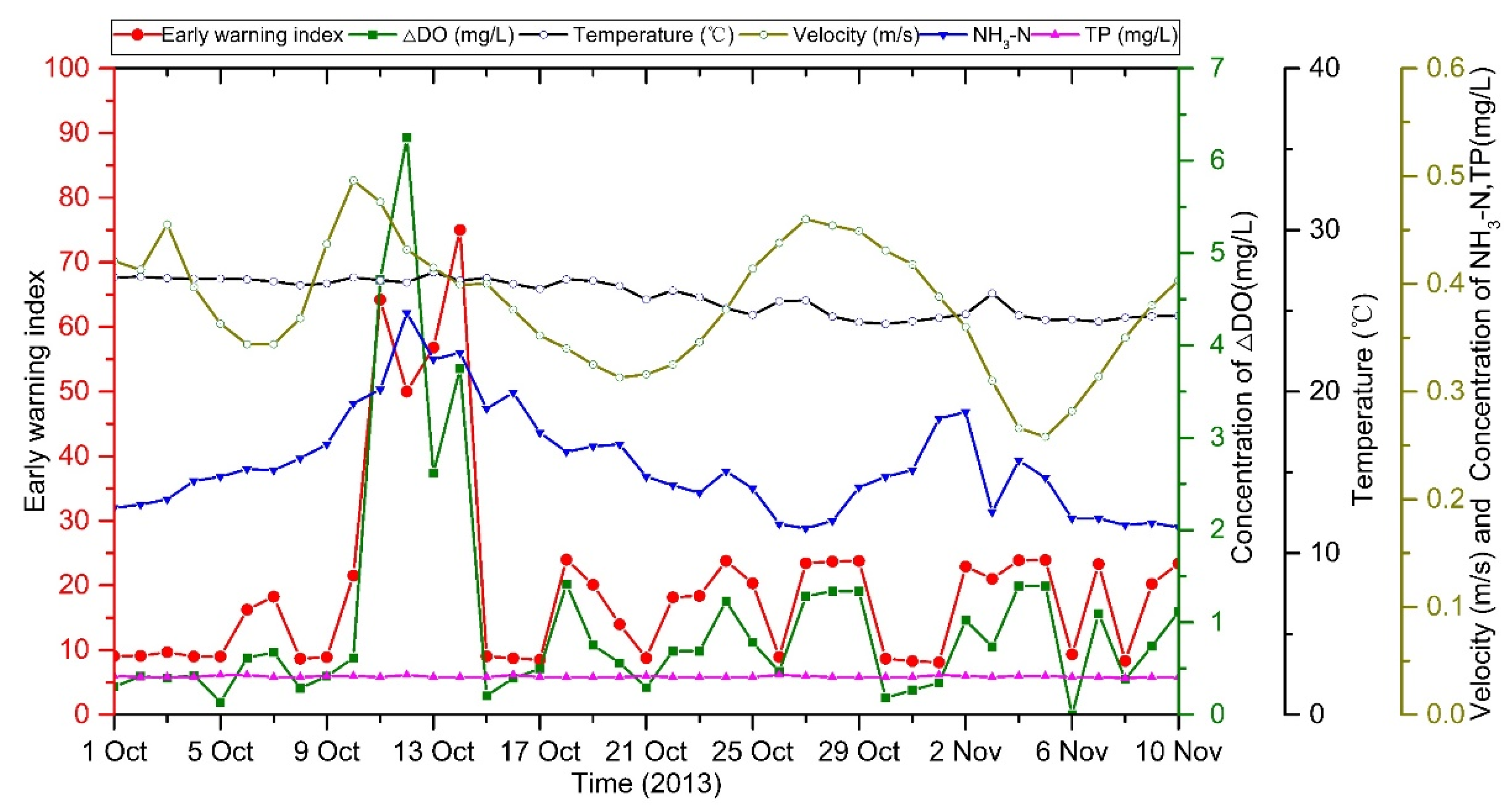
There was a false warning of the occurrence of an algae bloom. In October 2013, the warning index of DC station exceeded 50 and remained high for 4 consecutive days (Figure 7 and Figure 5d). However, no records of algae blooms were found during this period. Among all input variables, the steep increase of ∆DO from 1 mg/L to 2–6 mg/L after 10 October drove the elevated WQI. NH3-N and TP remained approximately 0.33 mg/L and 0.03 mg/L, respectively. The nutrient concentration contributed little to the variation in the WQI, as it was stably in the middle level of the fuzzy set. The velocity was at a medium level and the temperature was favorable for algae growth. Since the nutrients stay in middle or higher levels, the elevated ∆DO determined the increase in the early warning index.
However, at the PY station, there was neither a sustained increase in ∆DO during this false alarm period nor an increase in the warning index. The correlation between the DC and PY stations were rather low in the time series (Table 4), indicating little clues that could be referred to from the other station.
3.4. The Sensitivity of the Model Settings
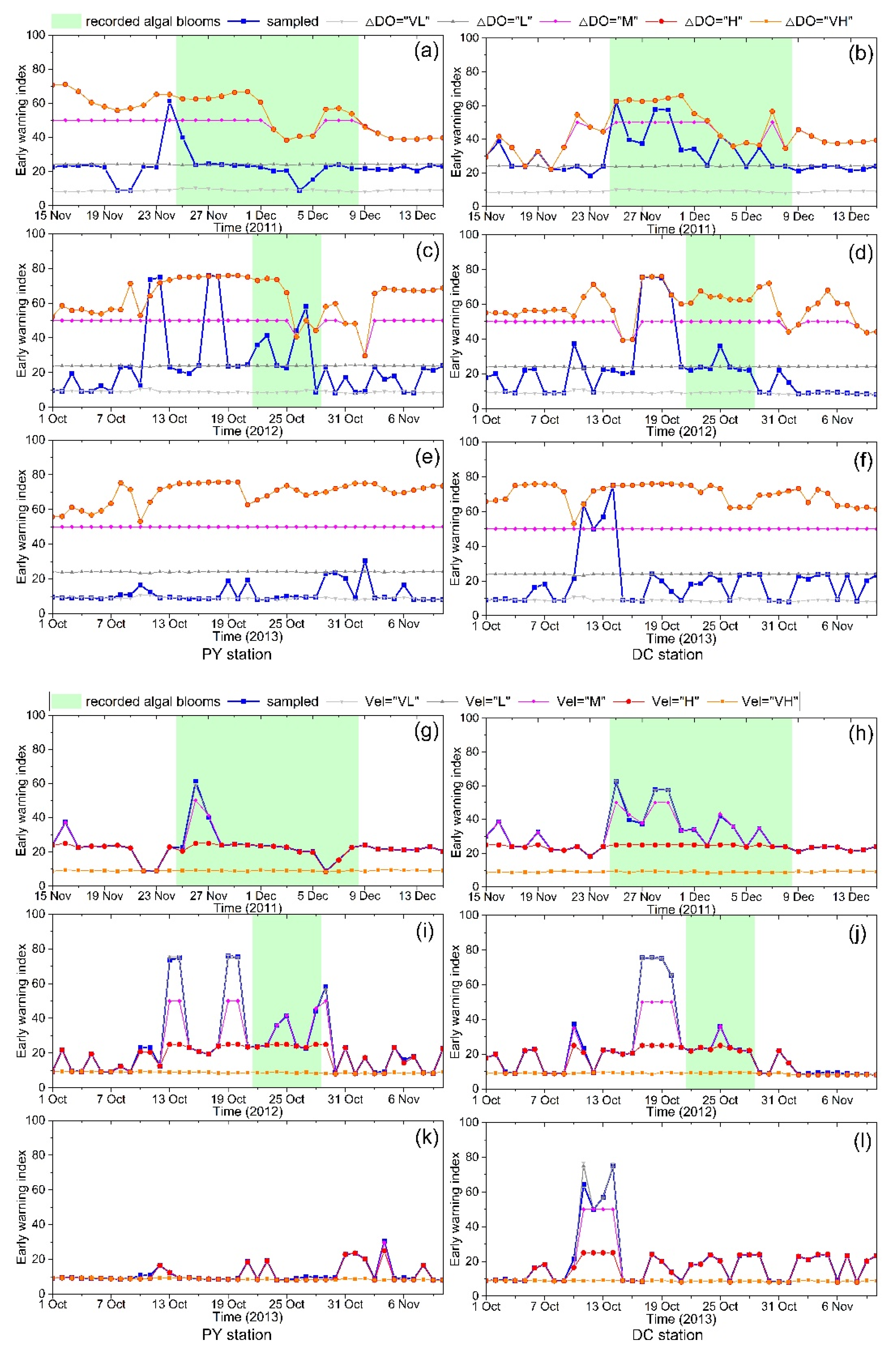
To further illustrate the sensitivity of the various input variables, we conducted a sensitivity analysis by setting the input variables to the median values of the VL, L, M, H, and VH levels (Table 2) and running the fuzzy logic model over the period of the bloom events under each setting. The results demonstrated that ∆DO was the most sensitive variable (Figure 8a–f). During the period prior to and during the bloom record, the warning index derived from the sampled value overlapped with the warning index derived from the ∆DO artificially assigned to the H and VH levels. However, when ∆DO was assigned with M, L, or VL values, the corresponding warning index never exceeded 50. Conversely, assigning the velocity value with VL, L, or M levels resulted in higher values of the warning index (Figure 8g–l). Aligned with the warning index derived from the validated simulation that mimicked the real system, the velocity remained in the ‘very low velocity’ or ‘low velocity’ subsets during the record of algae blooms, indicating that algae take advantage of calm hydrology conditions to accumulate.
3.5. Systematic Difference between Two Stations
The sluices’ operation can change the spread direction of the currents, leading the pollutants to enter the conservation area. The operation of the Yanzhou and Longwan sluices has changed the currents in this area from bidirectional to unidirectional (Figure 1), which has altered the intrusion of salty water and the spreading of waterborne pollutants. During the ebb phase (Figure 9a,c), the contaminated water from the Shiqiao River drains downstream (Figure 9a). In the DJL channel (location in Figure 1), the flow largely moves north (Figure 9c), indicating that the stronger ebb currents in the Shiqiao River inhibit the spread of its pollutants. Although the pollutants move downstream through the northern channel, the subsequent flood tide pushes the contaminated water back and potentially into the Shawan River due to the closure of the Longwan Sluice during the flood tidal phase (Figure 9d). Based on the distribution of ammonia in the simulation, the polluted water mass from the Shiqiao River could enter the Shawan River through the DJL channel and reach the intersection east of DC station (Figure 9b–d).
The simulated hydrodynamic feature may help to illustrate the difference between the two stations and shed light on the potential combined warning framework using data from both stations in the future. Within the limits of pollutant intrusion from the Shiqiao River due to the prior ebb tides, the DC station is more sensitive to the influence of tides from downstream regions. After initially exceeding warning thresholds, the warning index of the DC station experienced a slower and more gradual decrease (Figure 5e,f), which was mainly attributable to the slower recovery of velocity to the M or higher (Figure 8h,j,l) level. The intrusion of pollutants supplies the DC station with a water mass with different characteristics from that in most of the Shawan River in the further upstream part. However, the salinity of the auto-monitoring stations stayed at 0.01 during all sampled periods, which prevented further analysis of the extent and intensity of saltwater intrusion and further spatial estimation of water mass differences between the two stations.
Limited by data availability, the model’s output and algae bloom records were only compared quantitatively. The records only cover the bloom events that were detectable from the water’s color alone. This left the definition of ‘early’ open, as the algal community would have already rapidly increased in abundance before detection by visual observation. Given that South China has a nutrient-rich environment in which the water temperature rarely drops below 15 °C, the probability of algae blooms is theoretically high. However, the mechanisms and associated data sets necessary to provide early warning are complex. Among the variables of the fuzzy logic model, the ∆DO and velocity were the most sensitive driving variables.
4. Discussion
Based on our study, the periods with a high risk of algal blooms are in autumn. However, referring to publications about the downstream areas of our study site in the Pearl River Estuary, significant spatial variability has been highlighted. The growth of phytoplankton is influenced by underwater light availability, nutrients, stability of water column, and propagation of fronts [50]. Along the longitudinal axis of the Pearl River Estuary, it has higher productivity in summer and autumn [51]. Wind events have also added event-scale bloom in the records [52]. However, in river networks in the upstream part of the major estuary of the Pearl River and the adjacent small bay, further exploration was quite limited by the sparse data availability. In Shenzhen Bay, which is close to Hongkong, the strong runoff in May increases the pH and turbidity, thus inhibiting the flourishing of algal blooms in spring [53], which may be responsible for the absence of the significant spring bloom [54]. In summer, high temperatures and decreased residence time may also hinder the accumulation of algal bloom [55]. In winter, the growth is limited by temperature [53]. In summary, these conclusions support the high risk of algal blooms in autumn in river networks in this area.
In this study, we investigated the influence of tidal gates mainly in terms of the change in currents in tidal cycles. However, the impacts of tidal gates or other forms of dams may also alter water residence time, light conditions, and sediment trapping nutrient retention, thus changing primary productivity in these areas [56]. As an important part of the land–ocean aquatic continuum between upland ecosystems and the ocean, primary production is supposed to be a key element in the biochemical processes [57,58]. In the case of the Shawan–Shiqiao river network, residence time in most parts is reduced due to the one-direction tidal cycle. The release of nutrients from prior polluted sediments may depend on the age of dams [59] or duration of tidal gates’ operations. If we aim at reducing the possibility of algal blooms in long-term time scales, the altered ecosystem structure and function along river networks [60] and nutrients forms [61] should also be taken into account, which implies the need for long-term field observations and detailed process studies.
Even though the water quality of the Shawan channel has already met the type II water quality standards of surface water in China and serves as the drinking water source, the concentration of ammonia nitrogen and total phosphate are relatively high. In another word, in the clean water in the Shawan River, the ammonia concentration is classified into the ‘HIGH’ or even ‘VERY HIGH’ category of bloom risk, as same as the TP. Some scientists suggest that when the TN and TP exceed 0.2 mg/L and 0.02 mg/L [62], respectively, or 0.5 mg/L for TN and 0.02 mg/L for TP [63], the algal community no longer suffers from nutrient limiting. Under the condition that there are only criteria or online monitoring of the water quality index without attention paid to indexes of ecosystem status, to some extent, the un-matching between water quality standards and thresholds of algal growth may ‘hide’ the risk of blooms. In addition, the ratio between ammonia and nitrate merit consideration in the estimation of phytoplankton growth, since it has been observed that the presence of ammonia can inhibit the uptake of nitrate [64].
As drinking water is vital to maintaining people’s livelihood, health, and safety, the standard of a drinking water source is usually stricter than that of general water bodies [65]. It is necessary to analyze and predict the pollution risk to support the development of water source protection strategies, improving the scientific and risk predictability of water source protection [66,67]. However, because the algae bloom forecast is directly related to follow-up emergency management, which may involve multiple departments and enterprises, a false alarm might lead to increases in economic and social operation costs. Moreover, the untimely forecast may result in late response and disposal, threatening residents’ drinking water safety.
In the future, regarding the complexity of the forecast output, adoptions and integrations of forecasting tools of algal blooms may potentially vary among the demands of decision makers [68]. To better safeguard the operation of drinking water resource areas and water works, the forecasting systems should not only aim at achieving high chlorophyll-a or phytoplankton biomass risk prediction based on nutrients and hydrodynamical status, but also forecasting in the ecological sense [14] should be increasingly demanded. For example, effective assessment of certain toxins to be able to treat human health is necessary such as the MBio Toxin System [69] and MBio MC/CYN Toxin System [70]. Furthermore, studies on the excessive proliferation of phytoplankton (EPP) have advanced the understanding of the reproduction of algal cells [71] instead of high biomass that has resulted from reproduction processes. By integrating the previously scattered field sampling measurements with continuous observation or simulation in the spatial and temporal ranges, the development of a dense biomass of phytoplankton and related toxins may gain the potential to break through limitations in applications of early warning systems [72].
5. Conclusions
The growth of phytoplankton is affected by various factors that hinder the on-time detection of algae blooms. The present study selected several key factors (i.e., temperature, ΔDO, NH3-N, TP, and velocity) sampled by two auto-monitoring stations, together with simulated velocity from validated simulations, to build a fuzzy logic model. The built model was applied to produce an early warning index and hindcasted algae bloom events successfully. Considering the demands of management, the early warning index was additionally processed to provide a warning time duration, which reached critical success index and positive hit rate values of 0.5 and 0.9, respectively. The proposed prolongation time after the onset of alarm was 6–8 days. The threshold for the bloom onset was 60, with an appropriate subsequent threshold of 20 and 40, respectively, for the PY and DC stations. Under sufficient year-round nutrient and temperature conditions for algae growth, the ΔDO and velocity were the most important factors for producing accurate and timely forecasting.
The systematic differences between the PY and DC stations were revealed and discussed. The DC station, which was more influenced by the pollutants from prior ebb tides from the Shiqiao River, displayed a slower decrease in the warning index compared to the PY station, which is located further upstream and beyond the intrusion of pollutants during flood tides. The results suggest that spatial differences between sampling sites merit further exploration, particularly for sites located in the downstream–upstream sections, intersections between channels, or proximity to a pollution source. Additional parameters, such as biochemical markers of anthropogenic impacts, should be sampled and utilized for further analysis of water mass extents and data quality control of auto-monitoring sampling.
Author Contributions
Conceptualization, H.Y. and C.Z.; methodology, H.Y. and C.Z.; setting-up of the simulation, H.Y. and Y.Y.; validation, H.Y. and Y.Y.; analysis, C.Z., H.Y. and G.C.; writing—original draft preparation, H.Y.; writing—review and editing, C.Z. and Z.C.; visualization, H.Y., Y.Y. and Z.C.; supervision, funding acquisition, and project administration, F.Z.; All authors have read and agreed to the published version of the manuscript.
Funding
This work was funded by the Key-Area Research and Development Program of Guangdong Province (No. 2020B1111350001 and No. 2019B110205003) and the Basal Specific Research of the Central Public-Interest Scientific Institute (Grant No. PM-zx703-202004-141, Grant No. PM-zx097-202002-069).
Institutional Review Board Statement
Not applicable.
Informed Consent Statement
Not applicable.
Data Availability Statement
The availability of the sampled data obeys associated policies of the Panyu Ecological Environment Bureau. The simulated results presented in this study are available on request from the first author.
Acknowledgments
All authors are indebted to the Environmental Protection Monitoring Station of the Panyu District for providing the observed data. Authors are grateful to Zizhi Huang for formatting this manuscript and Hailong Zeng for technical support for figure plotting. The authors are obliged to the program ‘Origins, Early Warning and Prevention of Algae Blooms in Shawan Waterway, Panyu District, Guangzhou’ for organizing the sampling and data processing.
Conflicts of Interest
The authors declare that they have no known competing financial interests or personal relationships that could have appeared to influence the work reported in this paper.
References
- Amorim, C.A.; Moura, A.D.N. Ecological impacts of freshwater algal blooms on water quality, plankton biodiversity, structure, and ecosystem functioning. Sci. Total Environ. 2021, 758, 143605. [Google Scholar] [CrossRef] [PubMed]
- Sidabutar, T.; Srimariana, E.S.; Wouthuyzen, S. The potential role of eutrophication, tidal and climatic on the rise of algal bloom phenomenon in Jakarta Bay. In Proceedings of the IOP Conference Series: Earth and Environmental Science; IOP Publishing: Bristol, UK, 2020; Volume 429, p. 012021. [Google Scholar]
- Su, J.; Dai, M.; He, B.; Wang, L.; Gan, J.; Guo, X.; Zhao, H.; Yu, F. Tracing the origin of the oxygen-consuming organic matter in the hypoxic zone in a large eutrophic estuary: The lower reach of the Pearl River Estuary, China. Biogeosciences 2017, 14, 4085–4099. [Google Scholar] [CrossRef] [Green Version]
- Al-Yamani, F.Y.; Polikarpov, I.; Saburova, M. Marine life mortalities and Harmful Algal Blooms in the Northern Arabian Gulf. Aquat. Ecosyst. Health Manag. 2020, 23, 196–209. [Google Scholar] [CrossRef]
- Hallegraeff, G.M.; Anderson, D.M.; Belin, C.; Bottein, M.-Y.D.; Bresnan, E.; Chinain, M.; Enevoldsen, H.; Iwataki, M.; Karlson, B.; McKenzie, C.H.; et al. Perceived global increase in algal blooms is attributable to intensified monitoring and emerging bloom impacts. Commun. Earth Environ. 2021, 2, 1–10. [Google Scholar] [CrossRef]
- Berdalet, E.; Fleming, L.E.; Gowen, R.; Davidson, K.; Hess, P.; Backer, L.C.; Moore, S.K.; Hoagland, P.; Enevoldsen, H. Marine harmful algal blooms, human health and wellbeing: Challenges and opportunities in the 21st century. J. Mar. Biol. Assoc. U. K. 2016, 96, 61–91. [Google Scholar] [CrossRef] [Green Version]
- Watson, S.B.; Whitton, B.A.; Higgins, S.N.; Paerl, H.W.; Brooks, B.W.; Wehr, J.D. Harmful Algal Blooms; Elsevier Inc.: Amsterdam, The Netherlands, 2015; ISBN 9780123858771. [Google Scholar]
- Chen, N.; Hong, H.; Gao, X. Securing drinking water resources for a coastal city under global change: Scientific and institutional perspectives. Ocean Coast. Manag. 2021, 207, 104427. [Google Scholar] [CrossRef]
- Wang, C.; Kong, H.-N.; Wang, X.-Z.; He, S.-B.; Zheng, X.-Y.; Wu, D.-Y. Early-warning and prediction technology of harmful algal bloom: A review. J. Appl. Ecol. 2009, 20, 2813–2819. [Google Scholar]
- Huang, J.; Gao, J.F.; Mooij, W.M.; Hörmann, G.; Fohrer, N. A Comparison of Three Approaches to Predict Phytoplankton Biomass in Gonghu Bay of Lake Taihu. J. Environ. Inform. 2014, 24, 39–51. [Google Scholar] [CrossRef] [Green Version]
- Chen, Q.; Guan, T.; Yun, L.; Li, R.; Recknagel, F. Online forecasting chlorophyll a concentrations by an auto-regressive integrated moving average model: Feasibilities and potentials. Harmful Algae 2015, 43, 58–65. [Google Scholar] [CrossRef]
- Zhang, F.; Li, M.; Glibert, P.M.; Ahn, S.H. (Sophia) A three-dimensional mechanistic model of Prorocentrum minimum blooms in eutrophic Chesapeake Bay. Sci. Total Environ. 2021, 769, 144528. [Google Scholar] [CrossRef]
- Reguera, B.; Riobó, P.; Rodríguez, F.; Díaz, P.A.; Pizarro, G.; Paz, B.; Franco, J.M.; Blanco, J. Dinophysis Toxins: Causative Organisms, Distribution and Fate in Shellfish. Mar. Drugs 2014, 12, 394–461. [Google Scholar] [CrossRef] [PubMed]
- Glibert, P.M.; Allen, J.I.; Bouwman, L.; Brown, C.W.; Flynn, K.; Lewitus, A.J.; Madden, C.J. Modeling of HABs and eutrophication: Status, advances, challenges. J. Mar. Syst. 2010, 83, 262–275. [Google Scholar] [CrossRef]
- Stauffer, B.A.; Bowers, H.A.; Buckley, E.; Davis, T.W.; Johengen, T.H.; Kudela, R.; McManus, M.A.; Purcell, H.; Smith, G.J.; Woude, A.V.; et al. Considerations in Harmful Algal Bloom Research and Monitoring: Perspectives From a Consensus-Building Workshop and Technology Testing. Front. Mar. Sci. 2019, 6, 399. [Google Scholar] [CrossRef] [Green Version]
- Steffen, M.M.; Davis, T.W.; McKay, R.M.; Bullerjahn, G.S.; Krausfeldt, L.E.; Stough, J.M.; Neitzey, M.L.; Gilbert, N.E.; Boyer, G.L.; Johengen, T.H.; et al. Ecophysiological Examination of the Lake Erie Microcystis Bloom in 2014: Linkages between Biology and the Water Supply Shutdown of Toledo, OH. Environ. Sci. Technol. 2017, 51, 6745–6755. [Google Scholar] [CrossRef]
- Frolov, S.; Kudela, R.M.; Bellingham, J.G. Monitoring of harmful algal blooms in the era of diminishing resources: A case study of the U.S. West Coast. Harmful Algae 2013, 21–22, 1–12. [Google Scholar] [CrossRef]
- Franks, P.J.S. Recent Advances in Modelling of Harmful Algal Blooms. In Global Ecology and Oceanography of Harmful Algal Blooms; Glibert, P.M., Berdalet, E., Burford, M.A., Pitcher, G.C., Zhou, M., Eds.; Springer International Publishing: Cham, Switzerland, 2018; pp. 359–377. ISBN 978-3-319-70069-4. [Google Scholar]
- Zadeh, L.A. A video-enabled dynamic site planner. Inf. Control 1965, 8, 338. [Google Scholar] [CrossRef] [Green Version]
- Alhazaymeh, K.; Halim, S.A.; Salleh, A.R.; Hassan, N. Soft intuitionistic fuzzy sets. Appl. Math. Sci. 2012, 6, 2669–2680. [Google Scholar]
- Milanesi, G.S. Fuzzy logic, parity theories and two currencies valuation for emerging markets with de discount cash flow model. Financ. Mark. Valuat. 2019, 5, 69–94. [Google Scholar] [CrossRef]
- Aisjah, A.S.; Arifin, S. Maritime weather prediction using fuzzy logic in Java Sea for shipping feasibility. Int. J. Artif. Intell. 2013, 10, 112–122. [Google Scholar]
- Milton-Thompson, O.; Javadi, A.A.; Kapelan, Z.; Cahill, A.G.; Welch, L. Developing a fuzzy logic-based risk assessment for groundwater contamination from well integrity failure during hydraulic fracturing. Sci. Total Environ. 2021, 769, 145051. [Google Scholar] [CrossRef]
- Bruder, S.; Babbar-Sebens, M.; Tedesco, L.; Soyeux, E. Use of fuzzy logic models for prediction of taste and odor compounds in algal bloom-affected inland water bodies. Environ. Monit. Assess. 2014, 186, 1525–1545. [Google Scholar] [CrossRef] [PubMed]
- Kim, Y.; Shin, H.S.; Plummer, J.D. A wavelet-based autoregressive fuzzy model for forecasting algal blooms. Environ. Model. Softw. 2014, 62, 1–10. [Google Scholar] [CrossRef]
- Chi, W.; Zhang, X.; Zhang, W.; Bao, X.; Liu, Y.; Xiong, C.; Liu, J.; Zhang, Y. Impact of tidally induced residual circulations on chemical oxygen demand (COD) distribution in Laizhou Bay, China. Mar. Pollut. Bull. 2020, 151, 110811. [Google Scholar] [CrossRef] [PubMed]
- Choudhury, A.K. Relationship between N:P:Si ratio and phytoplankton community composition in a tropical estuarine mangrove ecosystem. Biogeosci. Discuss 2015, 12, 2307–2355. [Google Scholar] [CrossRef]
- Brzezinski, M.A. The Si:C:N ratio of marine diatoms: Interspecific variability and the effect of some environmental variables. J. Phycol. 2004, 21, 347–357. [Google Scholar] [CrossRef]
- Fisher, T.; Peele, E.; Ammerman, J.; Harding, L. Nutrient limitation of phytoplankton in Chesapeake Bay. Mar. Ecol. Prog. Ser. 1992, 82, 51–63. [Google Scholar] [CrossRef]
- Vidal, R.; Ma, Y.; Sastry, S.S. Principal component analysis. In Interdisciplinary Applied Mathematics; Springer Nature: Basingstoke, UK, 2016; Volume 40, pp. 25–62. [Google Scholar]
- ter Braak, C.J.F.; Verdonschot, P.F.M. Canonical correspondence analysis and related multivariate methods in aquatic ecology. Aquat. Sci. 1995, 57, 255–289. [Google Scholar] [CrossRef]
- Hamrick, J.M. A Three-Dimensional Environmental Fluid Dynamics Computer Code: Theoretical and Computational Aspects; Special Report in Applied Marine Science and Ocean Engineering; Virginia Institute of Marine Science, College of William and Mary: Williamsburg, VA, USA, 1992. [Google Scholar]
- Zhu, L.; Zhang, H.; Guo, L.; Huang, W.; Gong, W. Estimation of riverine sediment fate and transport timescales in a wide estuary with multiple sources. J. Mar. Syst. 2021, 214, 103488. [Google Scholar] [CrossRef]
- Shen, J.; Haas, L. Calculating age and residence time in the tidal York River using three-dimensional model experiments. Estuar. Coast. Shelf Sci. 2004, 61, 449–461. [Google Scholar] [CrossRef]
- Zhao, C.; Yang, H.; Fan, Z.; Zhu, L.; Wang, W.; Zeng, F. Impacts of Tide Gate Modulation on Ammonia Transport in a Semi-closed Estuary during the Dry Season—A Case Study at the Lianjiang River in South China. Water 2020, 12, 1945. [Google Scholar] [CrossRef]
- Hu, J.; Li, S. Modeling the mass fluxes and transformations of nutrients in the Pearl River Delta, China. J. Mar. Syst. 2009, 78, 146–167. [Google Scholar] [CrossRef]
- Pawlowicz, R.; Beardsley, B.; Lentz, S. Classical tidal harmonic analysis including error estimates in MATLAB using T_TIDE. Comput. Geosci. 2002, 28, 929–937. [Google Scholar] [CrossRef]
- Van Broekhoven, E.; De Baets, B. Fast and accurate center of gravity defuzzification of fuzzy system outputs defined on trapezoidal fuzzy partitions. Fuzzy Sets Syst. 2006, 157, 904–918. [Google Scholar] [CrossRef]
- Lee, J.; Hodgkiss, I.; Wong, K.; Lam, I. Real time observations of coastal algal blooms by an early warning system. Estuar. Coast. Shelf Sci. 2005, 65, 172–190. [Google Scholar] [CrossRef]
- Kong, F.; Song, L. Study on the Formation Process of Cyanobacteria Bloom and Its Environmental Characteristics; Science Press: Beijing, China, 2011; ISBN 978-7-03-030870-2. [Google Scholar]
- Zachariassen, K.E.; Cossins, A.R.; Bowler, K. Temperature Biology of Animals. J. Appl. Ecol. 1989, 26, 1092. [Google Scholar] [CrossRef]
- Montagnes, D.J.S.; Franklin, M. Effect of temperature on diatom volume, growth rate, and carbon and nitrogen content: Reconsidering some paradigms. Limnol. Oceanogr. 2001, 46, 2008–2018. [Google Scholar] [CrossRef] [Green Version]
- Liang, K.; Wang, X.; Zhang, D. Ecological conditions of diatom water bloom formulation in the middle and lower reach of the Hanjiang River and strategy for water bloom control. Environ. Sci. Technol. 2012, 35, 113–116. [Google Scholar]
- Holopainen, A.L.; Hovi, A.; Ronkko, J. Lotic algal communities and their metabolism in small forest brooks in the Nurmes area of eastern Finland. Aqua. Fenn. 1988, 18, 29–46. [Google Scholar]
- Pandey, A.; Parhi, D.R. MATLAB Simulation for Mobile Robot Navigation with Hurdles in Cluttered Environment Using Minimum Rule based Fuzzy Logic Controller. Procedia Technol. 2014, 14, 28–34. [Google Scholar] [CrossRef] [Green Version]
- Sherman, E.; Moore, J.K.; Primeau, F.; Tanouye, D. Temperature influence on phytoplankton community growth rates. Glob. Biogeochem. Cycles 2016, 30, 550–559. [Google Scholar] [CrossRef] [Green Version]
- Ross, T.J. Fuzzy Logic with Engineering Applications; Wiley: Hoboken, NJ, USA, 2010; ISBN 9780470743768. [Google Scholar]
- Mason, I. Dependence of the Critical Success Index on sample climate and threshold probability. Aust. Meteorol. Mag. 1989, 37, 75–81. [Google Scholar]
- Kurvers, R.H.J.M.; Krause, J.; Argenziano, G.; Zalaudek, I.; Wolf, M. Detection Accuracy of Collective Intelligence Assessments for Skin Cancer Diagnosis. JAMA Dermatol. 2015, 151, 1346–1353. [Google Scholar] [CrossRef]
- Zu, T.; Wang, D.; Gan, J.; Guan, W. On the role of wind and tide in generating variability of Pearl River plume during summer in a coupled wide estuary and shelf system. J. Mar. Syst. 2014, 136, 65–79. [Google Scholar] [CrossRef]
- Ye, H.; Chen, C.; Sun, Z.; Tang, S.; Song, X.; Yang, C.; Tian, L.; Liu, F. Estimation of the Primary Productivity in Pearl River Estuary Using MODIS Data. Estuaries Coasts 2015, 38, 506–518. [Google Scholar] [CrossRef]
- Yin, K.; Zhang, J.; Qian, P.-Y.; Jian, W.; Huang, L.; Chen, J.; Wu, M.C. Effect of wind events on phytoplankton blooms in the Pearl River estuary during summer. Cont. Shelf Res. 2004, 24, 1909–1923. [Google Scholar] [CrossRef]
- Yuan, C.; Xu, Z.; Zhang, X. Seasonal changes of phytoplankton in Shenzhen Bay from 2010 to 2011 and its relationship with environmental factors. Trans. Oceanol. Liminol. 2015, 1, 112–120. [Google Scholar] [CrossRef]
- Zhang, W.; Mu, S.S.; Zhang, Y.J.; Chen, K.M. Seasonal and interannual variations of flow discharge from Pearl River into sea. Water Sci. Eng. 2012, 5, 399–409. [Google Scholar] [CrossRef]
- Sun, J.; Lin, B.; Li, K.; Jiang, G. A modelling study of residence time and exposure time in the Pearl River Estuary, China. J. Hydro-Environ. Res. 2014, 8, 281–291. [Google Scholar] [CrossRef]
- Mendonça, R.; Kosten, S.; Sobek, S.; Barros, N.; Cole, J.J.; Tranvik, L.J.; Roland, F. Hydroelectric carbon sequestration. Nat. Geosci. 2012, 5, 838–840. [Google Scholar] [CrossRef]
- Regnier, P.; Friedlingstein, P.; Ciais, P.; MacKenzie, F.T.; Gruber, N.; Janssens, I.; Laruelle, G.; Lauerwald, R.; Luyssaert, S.; Andersson, A.J.; et al. Anthropogenic perturbation of the carbon fluxes from land to ocean. Nat. Geosci. 2013, 6, 597–607. [Google Scholar] [CrossRef]
- Battye, W.; Aneja, V.P.; Schlesinger, W.H. Is nitrogen the next carbon? Earth’s Futur. 2017, 5, 894–904. [Google Scholar] [CrossRef] [Green Version]
- Chen, Q.; Shi, W.; Huisman, J.; Maberly, S.C.; Zhang, J.; Yu, J.; Chen, Y.; Tonina, D.; Yi, Q. Hydropower reservoirs on the upper Mekong River modify nutrient bioavailability downstream. Natl. Sci. Rev. 2020, 7, 1449–1457. [Google Scholar] [CrossRef]
- Maavara, T.; Chen, Q.; Van Meter, K.; Brown, L.E.; Zhang, J.; Ni, J.; Zarfl, C. River dam impacts on biogeochemical cycling. Nat. Rev. Earth Environ. 2020, 1, 103–116. [Google Scholar] [CrossRef]
- Middelburg, J.J. Are nutrients retained by river damming? Natl. Sci. Rev. 2020, 7, 1458. [Google Scholar] [CrossRef]
- Heisler, J.; Glibert, P.; Burkholder, J.; Anderson, D.; Cochlan, W.; Dennison, W.; Dortch, Q.; Gobler, C.; Heil, C.; Humphries, E.; et al. Eutrophication and harmful algal blooms: A scientific consensus. Harmful Algae 2008, 8, 3–13. [Google Scholar] [CrossRef] [Green Version]
- Qin, B.; Wang, X.; Tang, X. Drinking water crisis caused by eutrophication and cyanobacterial bloom in Lake Taihu: Cause and measurement. Adv. Earth Sci. 2007, 22, 896–906. [Google Scholar]
- Poxleitner, M. Consequences of nitrogen enrichment on lake plankton, der Ludwig-Maximilians-Universität München. Ph.D. Thesis, der Ludwig-Maximilians-Universität München, Munich, Germany, 2016. [Google Scholar]
- Guo, T.; Yu, H.; Luo, J.; Li, Z. Safety problems in drinking water sources and standardized legal measures. Environ. Sci. Manag. 2010, 35, 14–16. [Google Scholar]
- He, T.; Luan, Z.; Guan, W. Discussion on the strategy of water source protection from the perspective of watershed ecosystem management. Environ. Prot. 2018, 46, 12–17. [Google Scholar]
- Zhang, H.; Wang, Y. Thoughts on boosting up-to-standard construction of major safe drinking water sources in China. China Water Resour. 2018, 9, 17–19. [Google Scholar]
- Gill, D.; Rowe, M.; Joshi, S.J. Fishing in greener waters: Understanding the impact of harmful algal blooms on Lake Erie anglers and the potential for adoption of a forecast model. J. Environ. Manag. 2018, 227, 248–255. [Google Scholar] [CrossRef] [PubMed]
- Reverté, L.; Campàs, M.; Yakes, B.J.; Deeds, J.R.; Katikou, P.; Kawatsu, K.; Lochhead, M.; Elliott, C.T.; Campbell, K. Tetrodotoxin detection in puffer fish by a sensitive planar waveguide immunosensor. Sens. Actuators B Chem. 2017, 253, 967–976. [Google Scholar] [CrossRef] [Green Version]
- Bickman, S.R.; Campbell, K.; Elliott, C.; Murphy, C.; O’Kennedy, R.; Papst, P.; Lochhead, M.J. An Innovative Portable Biosensor System for the Rapid Detection of Freshwater Cyanobacterial Algal Bloom Toxins. Environ. Sci. Technol. 2018, 52, 11691–11698. [Google Scholar] [CrossRef] [PubMed] [Green Version]
- Huisman, J.; Codd, G.A.; Paerl, H.W.; Ibelings, B.W.; Verspagen, J.M.H.; Visser, P.M. Cyanobacterial blooms. Nat. Rev. Microbiol. 2018, 16, 471–483. [Google Scholar] [CrossRef] [PubMed]
- Rousso, B.Z.; Bertone, E.; Stewart, R.; Hamilton, D.P. A systematic literature review of forecasting and predictive models for cyanobacteria blooms in freshwater lakes. Water Res. 2020, 182, 115959. [Google Scholar] [CrossRef] [PubMed]
Figure 1.
The bathymetry and locations of auto-monitoring stations, sampling sites, and tidal sluices in the Shawan–Shiqiao basin. The inset shows the distribution of the Guangdong–Hong Kong–Macau Greater Bay Area, Pearl River estuary, major tributaries of the Pearl River, together with the location of the Shawan–Shiqiao basin. The Longwan Sluice and Yanzhou Sluice are represented by red lines across the river. The two auto-monitoring sites, Panyu (PY) station and Dongchong (DC) station, are labeled by red dots. The two rivers are connected by the Dajiulv (DJL) channel. Purple triangles indicate the 10 sampling sites of biochemical variables. Yellow crosses indicate the 3 hydrology sampling locations for validation of the numerical simulation. Black arrows depict the direction of currents in a tidal cycle, with the Longwan Sluice opening at the flood phase and the Yanzhou Sluice opening at the ebb phase. The locations of drinking water source conservation areas are shaded in green.

Figure 2.
Comparison of simulated and observed velocity at three stations (see Figure 1 for locations).
Figure 2.
Comparison of simulated and observed velocity at three stations (see Figure 1 for locations).

Figure 3.
Schematic flow–diagram of the fuzzy model.

Figure 4.
Membership functions of five input variables (a–e) and membership used for defuzzification (f).
Figure 4.
Membership functions of five input variables (a–e) and membership used for defuzzification (f).

Figure 5.
The early warning indexes for PY Station (a) and DC station (d) from 2011 to 2012. Enlarged views of the two bloom periods are plotted for PY station (b,c) and DC station (e,f). The early warning indexes for the PY (g) and DC (h) stations are plotted for 2017–2019 when the blooms were absent. The onset threshold of the value 60 of the warning index is marked by blue dashed lines for the PY station (a,g) and DC station (d,h). In the enlarged views of bloom period (b,c,e,f), the recorded bloom periods are marked by grey shadows. The duration time of the bloom warning is depicted by pink shadows. The selected subsequent thresholds are shown in black crosses. The onset threshold (60) is depicted by a blue dashed line.

Figure 6.
Variations in CSI (a,b), TPR (c,d), and FAR (e,f) as a function of the subsequent threshold and prolongation time. The values of the PY station are plotted on the left panels and those of the DC station are on the right panels.
Figure 6.
Variations in CSI (a,b), TPR (c,d), and FAR (e,f) as a function of the subsequent threshold and prolongation time. The values of the PY station are plotted on the left panels and those of the DC station are on the right panels.

Figure 7.
Time series of the input variables and the warning index of the DC station during the false alarm period in October 2013.
Figure 7.
Time series of the input variables and the warning index of the DC station during the false alarm period in October 2013.

Figure 8.
Sensitivity of the warning index to various levels of ∆DO (a–f) and velocity (g–l) at the PY station (left panel) and the DC station (right panel). Recorded bloom periods are shaded in green. The warning index, based on original sampled data, is shown in blue.
Figure 8.
Sensitivity of the warning index to various levels of ∆DO (a–f) and velocity (g–l) at the PY station (left panel) and the DC station (right panel). Recorded bloom periods are shaded in green. The warning index, based on original sampled data, is shown in blue.

Figure 9.
Distribution of ammonia and velocity at ebb tide (a,c) and flood tide (b,d) in a tidal cycle.
Figure 9.
Distribution of ammonia and velocity at ebb tide (a,c) and flood tide (b,d) in a tidal cycle.


Table 1.
Results of the PCA analysis on data from three sampling campaigns.
| Campaign | PCA Components | Extracted Sums of Squared Loadings | Weighting Coefficients of Top 3 Factors | Relative Coefficients of Locations | |||||||
|---|---|---|---|---|---|---|---|---|---|---|---|
| Variance% | Cumulative Variance% | 1 | 2 | 3 | 4 | 1 | 2 | 3 | 4 | ||
| 1 | PCA1 | 45.63 | 46.63 | NH3-N (0.933) | TP (0.985) | Cl (0.820) | DO (−0.833) | S10 (7.988) | S9 (6.658) | S1 (−3.140) | S5 (−3.913) |
| PCA2 | 28.77 | 74.40 | CODMn (0.890) | Chl-a (0.763) | Vel (−0.594) | DO (−0.506) | S5 (3.167) | S1 (2.346) | S8 (−3.979) | S9 (−1.542) | |
| 2 | PCA1 | 54.569 | 54.569 | NH3-N (0.957) | Chl-a (0.845) | pH (−0.842) | SiO4 (−0.767) | S10 (11.25) | S9 (6.583) | S1 (−2.908) | S6 (−2.892) |
| PCA2 | 10.107 | 69.676 | Vel (0.706) | TP (0.471) | pH (0.493) | CODMn (−0.373) | S8 (1.773) | S1 (1.773) | S4 (−1.412) | S9 (−1.524) | |
| 3 | PCA1 | 60.357 | 60.357 | NH3-N (0.950) | TP (0.946) | DO (−1.969) | pH (−0.947) | S9 (13.514) | S10 (5.097) | S7 (−4.105) | S8 (−3.550) |
| PCA2 | 17.451 | 77.818 | CODMn (0.854) | Vel (0.628) | TP (0.274) | SiO4 (−0.495) | S7 (2.936) | S10 (0.825) | S3 (−3.409) | S2 (−0.906) | |
Table 2.
Input variables and the corresponding fuzzy sets.
| Very Low (VL) | Low (L) | Medium (M) | High (H) | Very High (VH) | Reference | |
|---|---|---|---|---|---|---|
| ΔDO (mg/L) | 0–1.5 | 0.5–2.5 | 1.5–3.5 | 2.5–4.5 | 3.5–6.0 | [39] |
| NH3-N (mg/L) | 0–0.075 | 0–0.15 | 0.075–0.225 | 0.15–0.30 | 0.225–2.0 | [40] |
| TP (mg/L) | 0–0.0075 | 0–0.015 | 0.0075–0.0225 | 0.015–0.03 | 0.0225–0.2 | |
| Tem (°C) | 10–15 | 10–20 | 15–25 | 20–30 | 25–35 | [41,42,43] |
| Vel (m/s) | 2–10 | 1–3 | 0.4–1.2 | 0.1–0.5 | 0–0.2 | [44] |
| Early warning index | 0–25 | 0–50 | 25–75 | 50–100 | 75–100 |
Table 3.
Fuzzy rules determining the fuzzy sets of early warning indexes.
| Rule Number | IF ‘Tem’ Is: | and IF ‘Vel’ Is: | and IF ‘WQI’ Is: | Then ‘EWI’ Is: |
|---|---|---|---|---|
| 1./2./3./ | VL | VL | (1.)VL/(2.)L/(3.)M/ | VL |
| 4./5. | (4.)H/(5.)VH | |||
| 6./7./8./ | VL | L | (6.)VL/(7.)L/(8.)M/ | VL |
| 9./10. | (9.)H/(10.)VH | |||
| 11./12./13./ | VL | M | (11.)VL/(12.)L/(13.)M/ | VL |
| 14./15. | (14.)H/(15.)VH | |||
| 16./17./18./ | VL | H | (16.)VL/(17.)L/(18.)M/ | VL |
| 19./20. | (19.)H/(20.)VH | |||
| 21./22./23./ | VL | VH | (21.)VL/(22.)L/(23.)M/ | VL |
| 24./25. | (24.)H/(25.)VH | |||
| 26./27./28./ | L | VL | (26.)VL/(27.)L/(28.)M/ | VL |
| 29./30. | (29.)H/(30.)VH | |||
| 31. | L | L | (31.)VL | VL |
| 32./33./ | L | M | (32.)L/(33.)M/ | L |
| 34./35./ | (34.)H/(35.)VH | |||
| 36. | L | H | (36.)VL | VL |
| 37./38./ | L | H | (37.)L/(38.)M/ | L |
| 39./40./ | (39.)H/(40.)VH | |||
| 41. | L | VH | (41.)VL | VL |
| 42./43./ | L | VL | (42.)L/(43.)M/ | L |
| 44./45. | (44.)H/(45.)VH | |||
| 46. | L | L | (46.)VL | VL |
| 47./48./ | L | M | (47.)L/(48.)M/ | L |
| 49./50./ | (49.)H/(50.)VH | |||
| 51./52./53./ | M | VL | (51.)VL/(52.)L/(53.)M/ | VL |
| 54./55. | (54.)H/(55.)VH | |||
| 56. | M | L | (56.)VL | VL |
| 57./58./ | M | L | (57.)L/(58.)M/ | L |
| 59./60./ | (59.)H/(60.)VH | |||
| 61. | M | M | (61.)VL | VL |
| 62. | M | M | (62.)L | L |
| 63./64./65. | M | M | (38.)M/(39.)H/(40.)VH | M |
| 66. | M | H | (66.)VL | VL |
| 67. | M | H | (67.)L | L |
| 68./69./70./ | M | H | (68.)M/(69.)H/(70.)VH | M |
| 71. | M | VH | (71.)VL | VL |
| 72. | M | VH | (72.)L | L |
| 73./74./75. | M | VH | (73.)M/(74.)H/(75.)VH | M |
| 76./77./78./ | H | VL | (76.)VL/(77.)L/(78.)M/ | |
| 79./80. | (79.)H/(80.)VH | |||
| 81. | H | L | (81.)VL | VL |
| 82./83./ | H | L | (82.)L/(83.)M/ | L |
| 84./85. | (84.)H/(85.)VH | |||
| 86. | H | M | (86.)VL | VL |
| 87. | H | M | (87.)L | L |
| 88./89./90./ | H | M | (88.)M/(89.)H/(90.)VH | M |
| 91. | H | H | (91.)VL | VL |
| 92. | H | H | (92.)L | L |
| 93. | H | H | (93.)M | M |
| 94./95. | H | H | (94.)H/(95.)VH | H |
| 96. | H | VH | (96.)VL | VL |
| 97. | H | VH | (97.)L | L |
| 98. | H | VH | (98.)M | M |
| 99./100. | H | VH | (99.)H/(100.)VH | H |
| 101./102./ | VH | VL | (101.)VL/(102.)L/ | VL |
| 103./104./ | (103.)M/(104.)H/ | |||
| 105. | (105.)VH | |||
| 106. | VH | L | (106.)VL | VL |
| 107./108./ | VH | L | (107.)L/(108.)M/ | L |
| 109./110. | (109.)H/(110.)VH | |||
| 111. | VH | M | (111.)VL | VL |
| 112. | VH | M | (112.)L | L |
| 113./114./ | VH | M | (113.)M/(114.)H/ | M |
| 115. | (115.)VH | |||
| 116. | VH | H | (116.)VL | VL |
| 117. | VH | H | (117.)L | L |
| 118. | VH | H | (118.)M | M |
| 119./120. | VH | H | (119.)H/(120.)VH | H |
| 121. | VH | H | (121.)VL | VL |
| 122. | VH | H | (122.)L | L |
| 123. | VH | H | (123.)M | M |
| 124. | VH | H | (124.)H | H |
| 125. | VH | VH | (125.)VH | VH |
Table 4.
Correlation coefficient of the warning index and driving variables of the fuzzy logic model between the PY and DC stations in different time periods.
Table 4.
Correlation coefficient of the warning index and driving variables of the fuzzy logic model between the PY and DC stations in different time periods.
| Time | Warning Index | ∆DO | NH3-N | TP | Temperature |
|---|---|---|---|---|---|
| 1 January 2011–31 December 2013 | 0.14 | 0.07 | 0.01 | −0.05 | 0.97 |
| 25 November 2011–8 December 2011 | 0.14 | 0.06 | 0.35 | 0.69 | 0.97 |
| 10 October 2012–28 October 2012 | 0.28 | 0.14 | 0.24 | 0.38 | 0.76 |
| 10 October 2013–20 October 2013 | 0.48 | 0.54 | 0.17 | −0.08 | 0.49 |
| 1 January 2017–31 December 2019 | 0.15 | 0.02 | 0.14 | 0.00 | 0.95 |
Publisher’s Note: MDPI stays neutral with regard to jurisdictional claims in published maps and institutional affiliations. |
© 2021 by the authors. Licensee MDPI, Basel, Switzerland. This article is an open access article distributed under the terms and conditions of the Creative Commons Attribution (CC BY) license (https://creativecommons.org/licenses/by/4.0/).
Share and Cite
MDPI and ACS Style
Yang, H.; Chen, Z.; Ye, Y.; Chen, G.; Zeng, F.; Zhao, C. A Fuzzy Logic Model for Early Warning of Algal Blooms in a Tidal-Influenced River. Water 2021, 13, 3118. https://doi.org/10.3390/w13213118
AMA Style
Yang H, Chen Z, Ye Y, Chen G, Zeng F, Zhao C. A Fuzzy Logic Model for Early Warning of Algal Blooms in a Tidal-Influenced River. Water. 2021; 13(21):3118. https://doi.org/10.3390/w13213118
Chicago/Turabian StyleYang, Hanjie, Zhaoting Chen, Yingxin Ye, Gang Chen, Fantang Zeng, and Changjin Zhao. 2021. "A Fuzzy Logic Model for Early Warning of Algal Blooms in a Tidal-Influenced River" Water 13, no. 21: 3118. https://doi.org/10.3390/w13213118
Note that from the first issue of 2016, this journal uses article numbers instead of page numbers. See further details here.