
A Hybrid MPI-OpenMP Parallel Algorithm for the Assessment of the Multifractal Spectrum of River Networks


1
Dipartimento di Fisica, Università della Calabria, Ponte P. Bucci, Cubo 31/C, 87036 Rende, Italy
2
Dipartimento di Matematica e Informatica, Università della Calabria, Ponte P. Bucci, Cubo 30/B, 87036 Rende, Italy
*
Author to whom correspondence should be addressed.
Water 2021, 13(21), 3122; https://doi.org/10.3390/w13213122
Submission received: 10 October 2021
/
Revised: 25 October 2021
/
Accepted: 3 November 2021
/
Published: 5 November 2021
(This article belongs to the Special Issue Advances in River Hydraulic Characterization)
Abstract
:The possibility to create a flood wave in a river network depends on the geometric properties of the river basin. Among the models that try to forecast the Instantaneous Unit Hydrograph (IUH) of rainfall precipitation, the so-called Multifractal Instantaneous Unit Hydrograph (MIUH) rather successfully connects the multifractal properties of the river basin to the observed IUH. Such properties can be assessed through different types of analysis (fixed-size algorithm, correlation integral, fixed-mass algorithm, sandbox algorithm, and so on). The fixed-mass algorithm is the one that produces the most precise estimate of the properties of the multifractal spectrum that are relevant for the MIUH model. However, a disadvantage of this method is that it requires very long computational times to produce the best possible results. In a previous work, we proposed a parallel version of the fixed-mass algorithm, which drastically reduced the computational times almost proportionally to the number of Central Processing Unit (CPU) cores available on the computational machine by using the Message Passing Interface (MPI), which is a standard for distributed memory clusters. In the present work, we further improved the code in order to include the use of the Open Multi-Processing (OpenMP) paradigm to facilitate the execution and improve the computational speed-up on single processor, multi-core workstations, which are much more common than multi-node clusters. Moreover, the assessment of the multifractal spectrum has also been improved through a direct computation method. Currently, to the best of our knowledge, this code represents the state-of-the-art for a fast evaluation of the multifractal properties of a river basin, and it opens up a new scenario for an effective flood forecast in reasonable computational times.
1. Introduction
The idea that the branched structures of river networks are multifractal and non-plane filling objects was first suggested by several authors [1,2,3]. The importance of the relation between the geometric characteristics of a river basin and its behavior under intense rainfall precipitation has been pointed out by Fiorentino et al. (2002) [4], who introduced the Fractal Instantaneous Unit Hydrograph (FIUH) model, in which they linked directly the lag time distribution function of a basin with its fractal dimension D, in the hypothesis that the a single fractal measure could characterize the whole river network. The model was further refined by De Bartolo et al. (2003) [5], who substituted the fractal dimension D of Fiorentino et al. (2002) with the generalized fractal dimension under the assumption that a river basin could be better represented as a multifractal object than as a simple fractal, thus proposing the so-called Multifractal Instantaneous Unit Hydrograph (MIUH). Moreover, the same authors showed, as in real cases, the MIUH can reproduce simulated hydrographs, which are in fairly good agreement with the observed ones.
Then, it becomes evident as the possibility to effectively forecast a possible flood peak happening in a river basin in the presence of rainfall precipitation is strictly connected with the need to evaluate the geometric properties of the river network in reasonable times, in particular, according to the MIUH model, its generalized dimension . The problem of determining the fractal dimensions of the basin can be summarized in the following steps: first, the map of the river basin is projected onto a plane, and its structure is represented by picking up (manually, or through automatic algorithms) a meaningful set of points lying on the branches of such 2D maps, the so-called net-points; second, a multifractal analysis is carried out in order to derive the generalized fractal dimensions , the sequence of Lipschitz–Hölder exponents and the multifractal spectrum .
The latter analysis can be performed through several numerical algorithms, which have been widely investigated in the past (see, for instance, De Bartolo et al. (2006) [6] and references therein for a discussion of the different approaches): fixed-size algorithms (FSA, e.g., box-counting and sandbox algorithms), the correlation integral method (CIM) introduced by Pawelzik and Schuster (1987) [7], and the fixed-mass algorithm (FMA) introduced initially by Badii and Politi (1984) [8]. Among the different approaches, the most promising one under the point of view of the possible application of an accurate determination of the parameters entering the MIUH model is the FMA. This happens because the generalized fractal dimension , present in the MIUH model, keeps account of the contribution of the regions of the basin less populated by net-points. Since both the FSAs and the CIM are based on the idea of counting the number of points falling inside a region of a given size, when such regions are filled up with few points, their contribution to the computation of high-order moments yields rather oscillating values due to the poor statistics, which, in turn, produce large errors in the determination of the generalized dimensions . On the other hand, the FMA considers the mass, as established a priori, and computes the characteristic sizes of the subset containing that mass, and therefore, it does not suffer from such a problem.
The drawback of the FMA is in the slowness of the computation. Where the analyses carried out numerically through the FSA and CIM produce the results in a computational time that scales linearly with the total number of points N of the multifractal set, the FMA requires a number of operations proportional to , which can be a huge CPU time even on modern fast processors (see below for a detailed explanation of this high number of operations). This produces a hardly solvable dilemma: on the one hand, modern Digital Elevation Models (DEMs) and Laser Imaging Detection and Ranging (LIDAR) techniques help in producing high-quality databases of river basins, with a very high number of net-points, which can improve the precision in the computation of the multifractal generalized dimensions, useful for the flood forecasts by using the MIUH model, for instance; on the other hand, the multifractal analysis that supplies the best results for the predictive models, the FMA, requires very long computational times, which limits the effectiveness of real-time forecast of flood peaks.
However, although the number of operations needed by the FMA cannot be easily decreased, it is a fact that modern computational supplies are typically equipped with multicore CPUs or are even multi-CPUs. Moreover, it is not truly difficult nowadays to assemble computational facilities by clustering several moderately expensive PCs interconnected with good network switches to allow the computation of parallelizable algorithms on a considerable amount of computational cores. In a previous article [9] (hereinafter we refer to this article as P1), we have discussed in detail a possible implementation of a parallel FMA by using the Message Passing Interface (MPI) paradigm [10], which is nowadays a standard for parallel numerical computations on distributed memory machines (such as the clusters of PCs cited above). Such a paradigm can also be used on shared memory machines, such as single-CPU workstations. However, better speed-ups can be obtained on single-node workstations by using the Open Multi-Processing (OpenMP) paradigm, which is also a consolidated standard for parallel numerical computations on shared-memory machines [11].
In the present article, we improved the parallel algorithm presented in P1 to include the use of OpenMP. This can improve the performance of the parallelization when the computation is carried out on single-CPU, multi-core workstations instead of clusters equipped with many computational nodes. Moreover, we further improved the analysis by modifying the algorithm to include a direct computation of the multifractal spectrum through the FMA [12]. In fact, in P1, the assessment of the multifractal spectra had been carried out by first computing the generalized dimensions through linear regressions from the computation of the moments, then obtaining the Lipschitz–Hölder exponents and the multifractal spectrum by using suitable numerical differentiation with a finite-difference approach. In the new version of the algorithm, instead, we used the direct procedure suggested by Mach et al. (1995) [12] for the direct computation of and . This allows an improvement of the precision in the computation of the latter two quantities with respect to P1.
Other than giving more precise and reliable results in the determination of the multifractal properties of the river networks, the code currently used in the present work exhibits an almost ideal scaling of the CPU time with the number of computational cores, thanks to the hybrid MPI/OpenMP parallelization, as will be shown in the section of the paper devoted to the presentation of the results and the discussion. The improvements in the computational speeds are remarkable and are limited only by the available number of cores present on the machine. It is worth noticing that the speed-up is rather good on both single-node, multi-core machines (like most workstations) and multi-node, multi-core clusters, as will be shown below.
The plan of the article is the following. In next section, Materials and Methods, we explain the serial FMA, the reasons for which it requires the very long computational times given by and the implementation of the direct computation of the Lipschitz–Hölder exponents and of the multifractal spectrum; then we summarize the parallelization of the algorithm with the MPI paradigm, proposed in P1, and the new OpenMP parallelization strategy implemented in the present work. In the third section, devoted to the results, we applied the proposed numerical methods to the computation of the properties of a theoretical multifractal set to evaluate the improvements of the application of the direct computation of the spectra, and then we analyze how the algorithm scales on different parallel configurations, with MPI only, OpenMP only, or with a hybrid MPI/OpenMP approach. Finally, in the section devoted to discussion, we draw some conclusions on the effectiveness of the proposed algorithm and the possible implications this may have on flood forecasts.
2. Materials and Methods
The multifractal analysis of a set of points is based on generating different partitions of the set itself and studying the scaling properties of the characteristic lengths with respect to the number of points (the so-called “measure” or “mass”) falling in each partition of the set. In particular, we assume that N is the total number of points of the set and that we can partition the set in non-overlapping cells. Let us call , , the size of the i-th cell and the total “mass” (in our case, the number of net-points) falling inside the same cell. For points belonging to a multifractal set, it is possible to show that the following relation must hold:
k being a constant, generally taken equal to 1, without losing generality.
In Equation (1), it is possible to show that, for each value of k, an infinite ensemble of solutions of the problem exists. The generalized fractal dimensions are related to those solutions through the relation:
When the solutions are known, the Lipschitz–Hölder exponents (or “spectrum of the singularities”) and multifractal spectrum are given through the relations:
The approach of the FSA (just to fix the concepts, we use as an example the procedure followed in the box-counting technique) to find the solutions of Equation (1) is to consider an ensemble of partitions: for each of them, the sizes of the cells are kept constant (, from which the name fixed-size algorithm), but this constant value decreases exponentially when changing the partition. By taking the logarithms of both sides of Equation (1), in the limit of a vanishing size s, one obtains:
with:
being the -th moment of the “mass” falling inside each box of the partition. Therefore, the solution , for a given set of values of q can be determined as the slope of the linear relation shown in Equation (4) for vanishing values of the size s. In practice, for each value of q, is computed through a linear regression of the logarithms of the moments with respect to the logarithm of the size s by considering . Once the solutions of Equation (1) have been determined, the generalized dimensions , the Lipschitz–Hölder exponents and the multifractal spectrum can be determined by using Relations (2) and (3).
For the FMA, the situation is the opposite. Instead of keeping the size as constant for each cell of the i-th partition, one fixes the “mass” (in our case, the number of net-points inside each cell of the partition) and computes the characteristic size of the cell containing that specific number of points. Again, the solution of Equation (1) can be determined by taking the logarithms of both sides of the equation and considering the limit for :
with:
Here, we took into account the fact that whenever . In this case, the solution of Relation (1) is obtained by fixing a set of values for and finding the corresponding value of q as the slope of the linear relation shown in Equation (6), which yields the value of . The latter operation can be carried out as a linear regression of the logarithms of the moments as a function of the logarithms of the “mass” p (always for ).
In practice, the FMA works in the following way: (i) first, one fixes a set of values for in a given interval and a discrete set of values for p (between 1 and ); (ii) for a given value of p, the size of the circle containing a “mass” equal to p is computed by calculating, for each of the N points of the set, the first p-th nearest neighbors; (iii) once the different radii of the circles containing at most p values are found, for each point, one can compute the moments (Equation (7)) for all specified values of . The true bottleneck of the algorithm lies in the point (ii): since for each point of the set, the reciprocal distances for all the points must be computed, and, subsequently, the vector of such quantities must be sorted in increasing order, in such a way that the p-th element of the vector represents the radius of the cell containing, for each point, the p nearest neighbors. The sorting operation can be carried out in a “fast” way, in operations, for instance, with a heap-sort algorithm, but the computation of the distances between each couple of points requires about operations. Therefore, the total number of operations required for a set containing N points is:
which is a really huge number for high values of N, much higher than the simple counting operations needed by many of the FSAs.
On the other hand, the FMA is superior to the FSAs, in many respects, at least for the assessment of the multifractal properties of river networks, as shown by [6]. In fact, as cited above, the main quantity connected to the geometrical properties of the set and entering the MIUH model is the quantity , which corresponds to the zones of the fractal set where the points are more rarefied. This also corresponds to the maximum value of the Lipschitz–Hölder exponent . Therefore, the precise determination of the generalized dimensions in the zones where the number of points is more rarefied is crucial for the possibility of obtaining an optimal forecast in the MIUH model. Unfortunately, FSAs exhibit strong oscillations in the computation of the moments (Equation (5)) in the more rarefied zones of the set due to poor statistics (because the size is fixed, and the “mass” falling in the cell of the partition is “counted”). On the other hand, FMA does not suffer from such a problem since, in that case, the number of points is fixed and the size of the cell computed accordingly. Therefore, the assessment of the with the FMA is much more precise than with FSA, i.e., the first is more suitable to be used for flood forecasting models like the MIUH.
This represents a problem, in view of the fact that modern DEM and LIDAR techniques allow the extraction of a quite high number of net-points, which would help improve the predictive quality of the MIUH. Moreover, recently, an attempt has been made to investigate scaling laws in flow patterns obtained by numerically simulating the behavior of a river basin through a 2-dimensional Shallow-Water approach [13]. In such cases, virtually every point of the numerical grid can be considered as a net-point, thus requiring a significant numerical effort to characterize the multifractal properties of the basin under study.
A possible solution for the problem of the long computational times for high values of N, as evidenced in P1, is the parallelization of the FMA. In P1, we proposed a possible parallelization of the algorithm based on the Message Passing Interface (MPI) paradigm. This computational model has become a standard for parallel computing, especially on distributed memory machines. It requires that the computations needed by the numerical code can be divided among a team of numerical cores participating in the parallel computation. This condition is realized by starting at the same time separated instances of a process on the different cores and whenever one of the cores needs to be informed on the status of the computation carried out by other cores, the processes communicate among them through a Local Area Network (LAN) interconnection. This is quite effective on distributed memory machines, in which several independent nodes are reciprocally interconnected through a LAN, but it can, in principle, also work on single-node machines by running the different instances of the code on the different cores of a single, multi-core CPU. However, simulating the presence of a network communication on such machines, where no network is necessary since the cores communicate through the physical bus of the processor, generates some latency in the communications. In P1, we measured the speed-up of the code by finding a fairly good scaling of the computational speed with the number of processors , although the speed-up curve has a linear trend (i.e., very close to the theoretical scaling) for smaller only and tends to saturate for an increasing number of computational cores due to the above-cited latency in the communications.
For this reason, we implemented the OpenMP directives into the code in order to improve the computational speeds on shared memory machines. This paradigm is nowadays a standard for this kind of computation, and it works through the use of “directives”, which can be considered as simple comments, and therefore ignored, unless the compiler is specifically instructed to consider them with special compilation flags. The parallelization in OpenMP works in a fork/join implementation: a single process executing the code forks in a sequence of “threads” (whose number can be specified through environment variables before the execution of the run) when it encounters # pragma omp parallel directives, which marks the beginning of a region of the code that can be executed in parallel. The threads join at the end of the parallel region, and the execution of the code continues as a serial run. The real effectiveness of such a paradigm depends strictly on the problem solved by the code: codes involving large, time-consuming loops can be parallelized much more effectively with respect to a sequence of small loops due to the latency in the creation of the threads that, being almost independent processes, can require a fairly large amount of CPU time to be created.
However, in the case of the FMA, the main bottleneck resides in the big loop that computes the mutual distances between the net-points and sorts them. This represents an almost ideal case for an OpenMP implementation. As we will show below, indeed, the improvements obtained with the adoption of the OpenMP paradigm are relevant with respect to the pure MPI case. Moreover, the application of both the paradigms (MPI and OpenMP) is not at all new in hydraulics applications (see, for instance, [14,15,16] for relevant hydraulic applications, albeit in different contexts).
Moreover, beyond improving the computational times of the code on single-node, multi-core machines, we also improved the precision in the determination of the multifractal spectrum by including the direct computation of the Lipschitz–Hölder exponents and multifractal spectrum in the code, adopting the technique first introduced by Mach et al. (1995) [12]. In P1, for instance, once the solutions of Equation (1) are known, the determination of and was carried out by computing the derivatives in Equation (3.1) by using a second-order finite differences method with a non-uniform stencil due to the fact that the values of q are chosen uniformly distributed in a given interval, but the , which are numerically calculated from the linear regression of the moments as in Equation (6), are not equally spaced (for details about the used formulae, see P1). This introduces some amount of numerical error, which makes the determination of and less precise. Instead, the direct computation method introduced in [12] computes the spectrum of the singularities and the multifractal one through the relations:
where:
which represents a normalized measure of the characteristic lengths to the power . The advantage of the above method is that it does not require any numerical differentiation and a linear regression between the quantities at the left hand side of Equation (8) as a function of is enough to compute both and . A detailed derivation of Equation (8) is shown in Appendix A.
The parallelization strategy adopted in order to divide the computational effort among the different nodes and cores of the computational machine was oriented to accelerate the computation of the mutual distances among the net-points, which is a algorithm. By following the method pursued in P1, we read the file with all the net-points on all the MPI processes; however, the computation of the distances is carried out on different subsets of points on each computational node. The parallelization with OpenMP follows the same idea: on each node, the loop for the computation of the distances is further divided on each computational core through a #pragma omp parallel directive by suitably specifying the different role (private or shared) of the loop variables.
When the mutual distances of each point from the others have been calculated, such a vector is sorted in ascending order with a heap-sort method. This operation is still carried out in parallel for each node and core. By sorting the vector of the distances, we ensure that the p-th element of such a vector corresponds to the radius of the circle containing at most p nearest neighbors. At this point, the contribution to the moments in Equations (7), (8.1) and (8.2) is executed separately on each core. At this point, two “reduce” operations—the first to add-up the contribution computed on each core through a pragma opm reduce directive and the second to sum the contribution of each single node through a MPI_REDUCE operation—are performed in order to evaluate the final values of the different moments.
Finally, the linear regressions necessary to compute the values of , and through the direct method [12] are calculated through a python script. Examples of the results obtained in the case of a deterministic multifractal are shown in the next section.
3. Results
In this section, we analyze the results of the application of the direct method to a deterministic multifractal for the determination of , and to assess the precision of the method in a case in which the theoretical solution of the problem is known. After that, we study the effectiveness of the parallel algorithm in the case of the pure OpenMP implementation, which should mimic the most common case of a machine with a single CPU and many computational cores; then we analyze the performances of the pure MPI parallel case, which should be closer to the case of a multi-node machine.
3.1. Testing the Direct Method against a Deterministic Multifractal
Here we analyze whether the direct method for the FMA provides good results in terms of the precision in the assessment of the relevant multifractal quantities , and . To accomplish this aim, we build up a deterministic multifractal through an iterative procedure, whose multifractal properties can be easily evaluated, to compare with the results of the numerical algorithm.
To do this, we use the same deterministic multifractal used in P1 in order to compare the results obtained in P1, where the multifractal spectrum was obtained through numerical differentiation and not through the direct method. We briefly recall here the construction of the deterministic multifractal. Major details can be found in P1 and [17].
We start from a square and consider the following transformations:
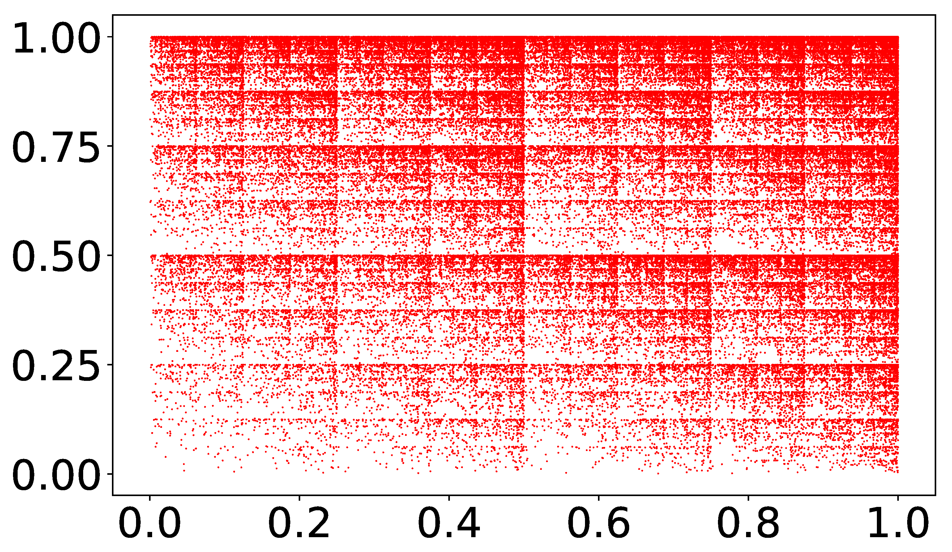
In practice, the original square, with a side equal to 1 partitioned into 4 squares, each having sides equal to and the transformations , map a generic point into another point belonging to one of the 4 squares of side . We assign to such mapping some probability to happen, for instance: , for . Notice that: . This means that the transformation can happen with a probability equal to , with a probability , and so on. We then generate an ensemble of N random numbers in the interval [0,1], and we apply the transformation if the random number falls in one of the intervals: [0,1/10], [1/10,3/10], [3/10,6/10] and [6/10,1]. Since the widths of such intervals are just equal to , each transformation will happen with such a probability. The result of such a construction for the case of net-points is shown in Figure 1.
It can be shown that, for the theoretical multifractal just described, the values of can be obtained for each value of q by the analytical relation:
which yields the result:
from which one can obtain the theoretical behaviour of and through Relation ( 3):
where the quantity is defined in a way analogous to Equation (9):
One can notice here that: , which, again, is a property analogous to the one given in Appendix A, Equation (A4), for the quantity defined in Equation (9).
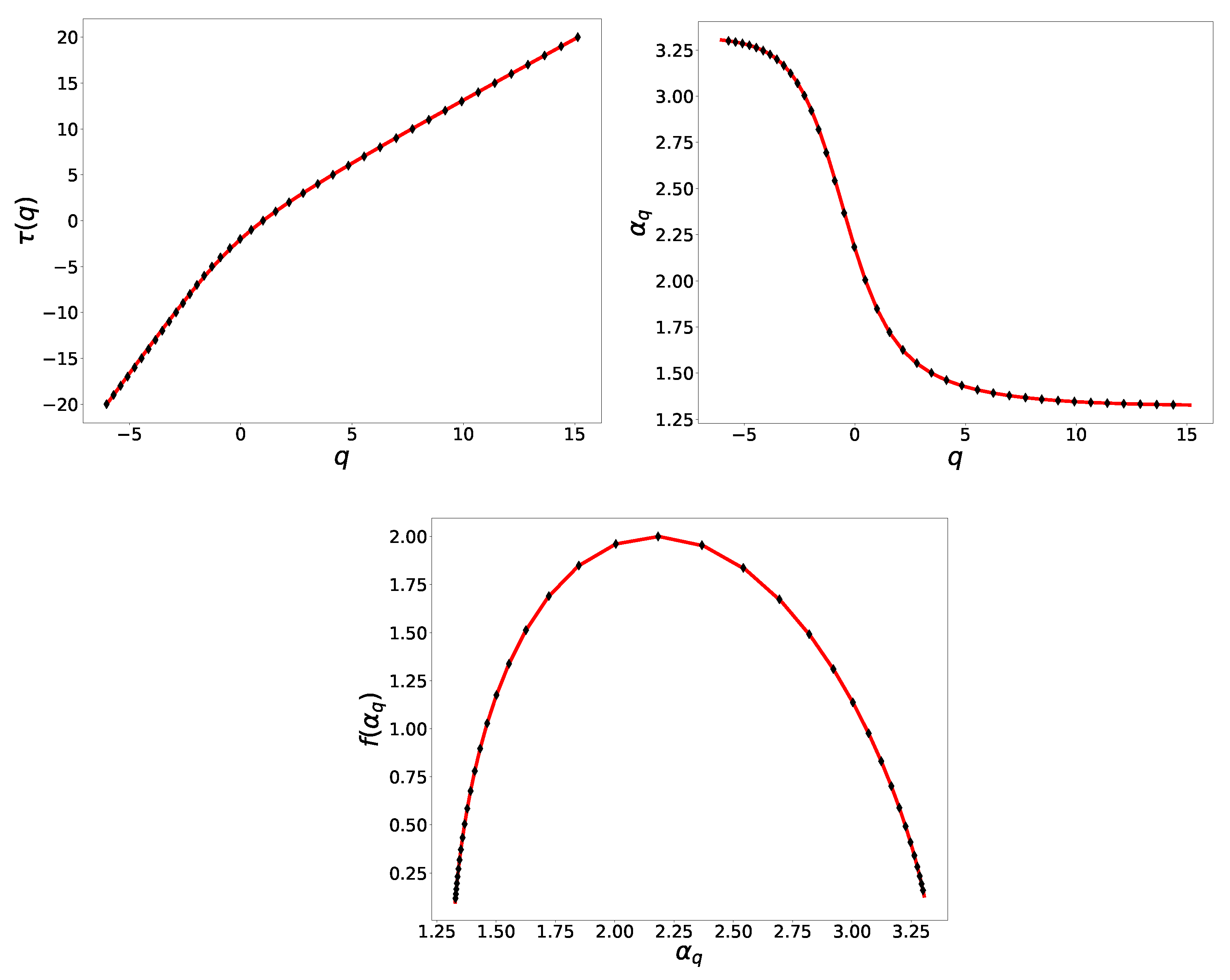
In the different panels of Figure 2, one can see the comparison between the plots of , and obtained through the parallel FMA (diamonds) and the theoretical values given by Equations (11) and (12) (black, solid line). It is evident as the two results are practically identical, thus suggesting that the numerical procedure, together with the direct method, produces a very precise assessment of the multifractal properties of the set under study. One can compare such results with the one obtained in P1 (see Figure 3 in P1: https://link.springer.com/book/10.1007/978-3-030-39081-5 30 October 2021) through numerical differentiation to realize how the direct method allows a much more precise assessment of the multifractal spectrum.
3.2. Testing the Effectiveness of the Parallelization Strategy
After verifying that the parallel algorithm yields fairly good results, we want to verify the improvements the parallel version of the code brings about in view of a possible application of the method for the flood forecast.
We define the computational speed-up in the usual form:
where is the CPU time for a serial run, whilst is the execution time in parallel on n cores. For a perfectly parallelized code, . Such theoretical value in most cases can be typically only reached on a low number of cores due to several effects. On single-node, multi-core machines, the limited bandwidth of the memory bus, through which all inter-node communications pass, represents a bottleneck when a large number of cores have to communicate with each other. The situation is even worse on multi-nodes systems since all communications pass through the LAN, which is generally much slower than the memory bus of the motherboard. Therefore, the theoretical scaling is only reachable for those algorithms that require very few or no communications at all (although, in some very special cases, even a superlinear scaling, namely better than the theoretical one, is possible).
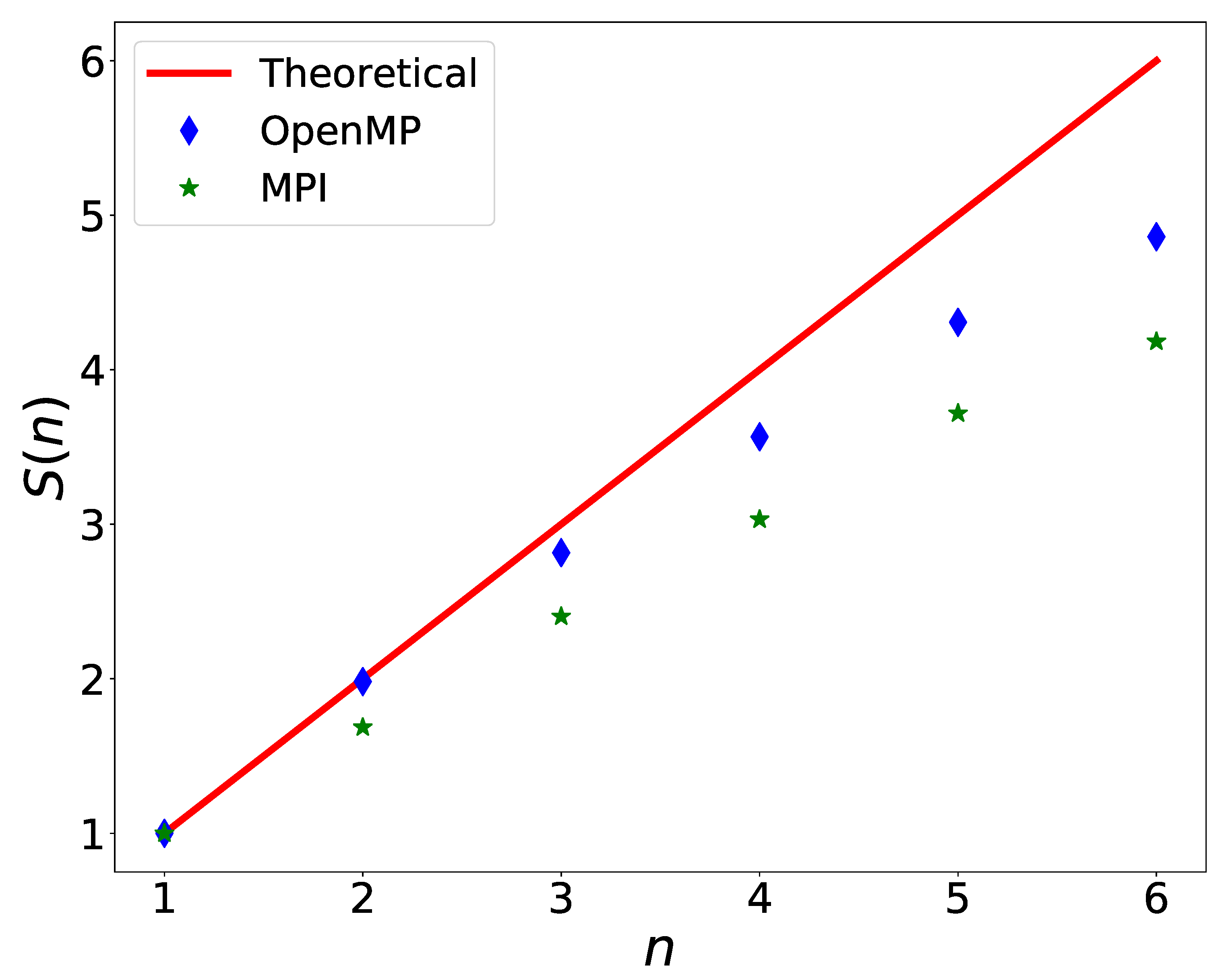
In Figure 3, the theoretical () speed-up (red solid red line), the one obtained by using OpenMP only (blue diamonds) and the one obtained by using only MPI (green stars) are shown for comparison as a function of the number of cores. The simulations have been run on a single-node, 6-core workstation equipped with an Intel i7-10710U CPU with a peak frequency of 4.7 GHz. It is evident that the parallelization with OpenMP considerably improves the performance with respect to the pure MPI case, giving a speed-up much closer to the theoretical one.
Finally, we analyzed the speed-up that can be obtained on a multi-node cluster to estimate the parallel performances of the code when compared with the single-node, single-CPU case treated above. In this case, the code was run on a cluster composed of 32 computational nodes. Each node is equipped with 2 Intel Xeon E5-2680v2 CPUs with 10 cores/CPU at a peak speed of 2.8 GHz and 128 GB of RAM/node. We ran the code with a number net-points in 10 different configurations, as reported in Table 1. One run was executed with the serial version of the code (Run 0 in Table 1), and the reported CPU-time was 1203 s. All the other 10 runs were executed with different combinations of MPI processes and OpenMP threads in order to analyze whether the OpenMP parallelization can effectively enhance the computation. For instance, Runs 4, 5 and 6 were all executed with the same number of total processes (here, we consider an OpenMP thread as an actual process, although this is true only during the time in which the processes fork). In this case, Run 4 was a pure MPI run, with 8 MPI processes and 1 OpenMP thread. In this case, the CPU-time used for the computation was 220 s, which is quite distant from the theoretical scaling: serial time/ number of processor ∼150.38 s. Then, Run 5 was a hybrid MPI/OpenMP code, always involving the execution of 8 processes in total (4 MPI processes and 2 OpenMP threads). In this case, the CPU time used by the code was considerably lower at 181 s. The last run, Run 6, was a pure OpenMP run, with 1 MPI process and 8 OpenMP threads. In this case, the measured CPU time was 156 s, which is very close to the theoretical scaling of 150.38 s reported above. In all other cases (4 and 16 total processes), we found the same behavior, namely the code benefits some further speed-up from the introduction of the OpenMP directives with respect to the pure MPI case.
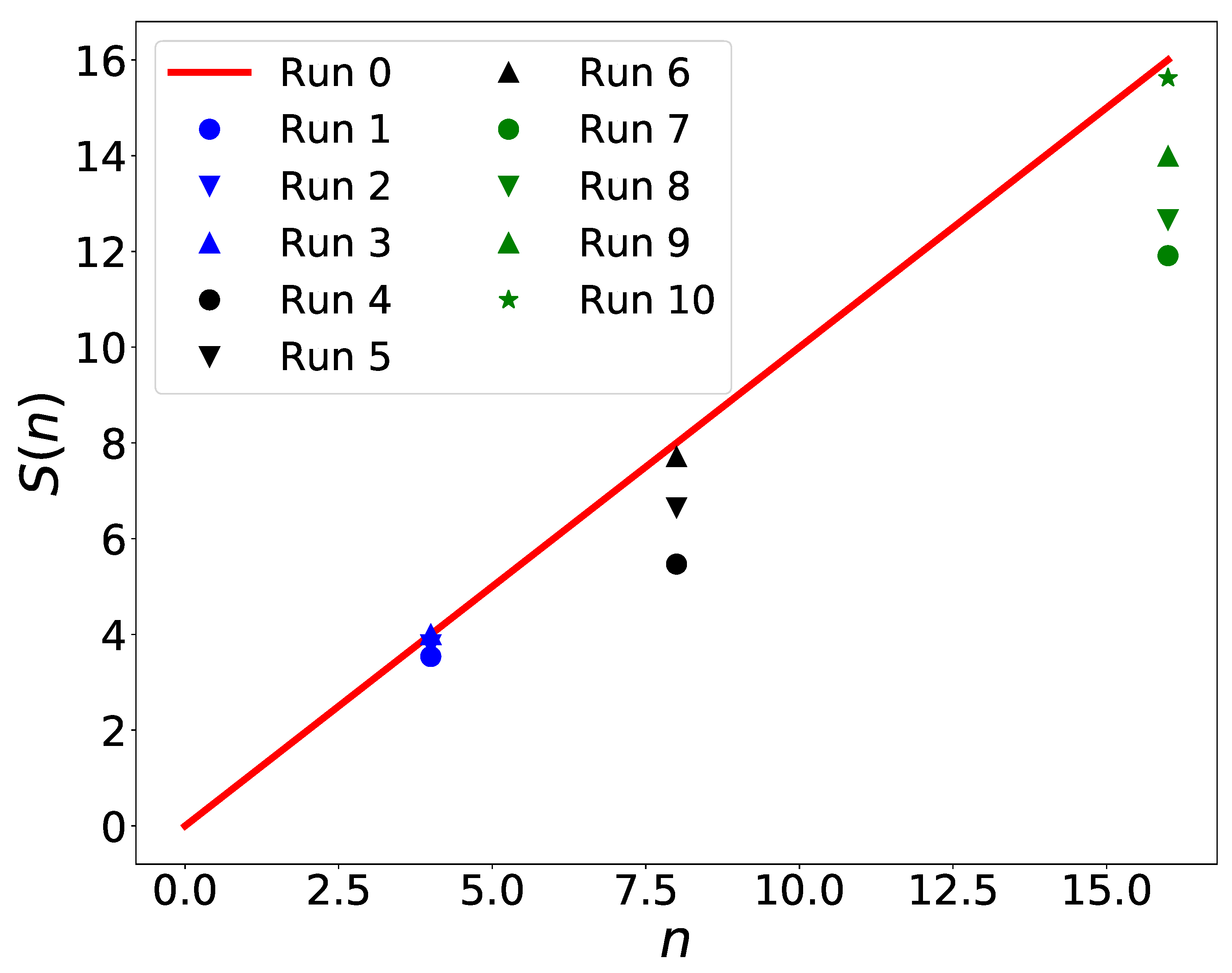
The results contained in Table 1 are shown in terms of the computational speed-up in Figure 4. The red solid line represents the theoretical speed-up, whilst the different points are the speed-ups measured for the different Runs (listed in the legend of the Figure) in Table 1. For the cases with 4, 8 and 16 total processes, the points that are closer to the theoretical speed-up are the ones with the highest number of OpenMP threads (Runs 3, 6 and 10, respectively).
These findings, again, confirm that OpenMP drastically reduces the latences of the communications by increasing considerably the speed-up of the computations with respect to the simple MPI case. Moreover, Run 3 and 4 show that whenever possible, the higher the number of used OpenMP threads, the higher the speed-up is. Of course, this situation may soon saturate due to the limited amount of cores available on each CPU and the fact that all cores of the CPU share the same memory bus, which can become a bottleneck when each core has to access large parts of the memory, and this may be particularly critical for a much larger number of net-points. Some numerical experiments are needed, in each case, to establish the best combination of MPI/OpenMP cores to use to minimize the execution speed.
4. Discussion
In the past, several studies have shown that river networks are non-plane filling, multifractal structures and that their geometric properties strongly influence the behaviour of the instantaneous hydrograph during rainfall precipitation. Models such as the MIUH, discussed above, require detailed knowledge of the generalized dimensions of the river basin. In the past, several authors have shown that, among the several possible methods, the FMA was the one yielding the most precise assessment of the multifractal measures for hydrological applications. However, the FMA has the disadvantage, with respect to other methods, to require rather long computational times to accomplish the analysis.
In order to tackle this problem, we transformed a serial code, developed in the past to implement the FMA, into a parallel code to reduce the computational times. In fact, nowadays, modern computers have an increasingly higher number of computational cores, which can be used together to speed-up the computation. The present study investigates the possibility to improve this already existing parallel (pure MPI) numerical code to include the parallelization through the OpenMP paradigm, which is nowadays a standard for parallel computations on shared memory machines. Although the code parallelized with MPI allowed the parallel execution not only on multi-node clusters but also on single-node workstations, we have shown here that the adoption of the OpenMP parallel directives are quite beneficial for the speed-up of the computation. In any case, the code can be run in a hybrid mode by using the MPI library to manage the execution on multi-node clusters and OpenMP to ensure the best possible execution time on the single node. Our results have shown that the latter yields the best results in terms of computational speed-up in the case of distributed memory machines.
As an example, the serial version of the code in the case of net-points takes about 1203 CPU seconds to be executed according to the results shown in Table 1. This means that, if we had net-points, namely 10 times more than our simple study-case, by retaining only the most important terms in the number of operations (), we can expect that the CPU time needed by the serial version of the code would be about 120300 CPU seconds, namely around 33.5 CPU hours. If we have a machine with 16 cores available, for instance, due to the quasi-linear scaling of the code in the hybrid MPI/OpenMP case, we could obtain the results in just 2.5 CPU hours. This is, of course, not an ideal situation, but, in principle, the speed-up is limited only by the number of cores available on the machine. The pure MPI implementation realized in P1, for instance, would yield an almost ideal speed-up for a lower number of processes only due to the latency of the network interconnection. This situation can be minimized by using the hybrid MPI/OpenMP implementation of the code described in the present work.
Along with the improvements in the parallelism of the computation, another considerable step towards a better assessment of the generalized dimensions of a river basin was taken by introducing a direct method for the computation of the Lipschitz–Hölder exponents and the multifractal spectrum. This allowed us to obtain, at least for the known case of a deterministic multifractal, a very precise assessment of those quantities, better than that obtained in the past through numerical differentiation.
5. Conclusions
The possibility of studying the multifractal properties of river networks through this code opens up, in our opinion, a new scenario in the application of models such as the MIUH for flood forecasting. In fact, single-node, multi-core CPUs are nowadays present even on desktop workstations. The parallelization of the code proposed here can exploit the presence of the different cores on the CPU in an optimal way by effectively dividing the computational time by the number of available cores. The situation can be even further improved if more nodes are available, thanks to the MPI implementation.
However, some further improvements are still possible. Nowadays, an increasing amount of codes for scientific analysis are implementing the possibility to execute the heaviest numerical tasks on Graphics Processing Units (GPUs), which are equipped with a huge amount of computational cores, albeit with less extended capabilities with respect to the cores of the CPUs. Typical paradigms for exploiting the computational power of the GPUs are: CUDA, developed by Nvidia; OpenACC, developed by Cray, CAPS, Nvidia and PGI; OpenGL, developed by SGI. We are currently developing a CUDA version of the parallel FMA in order to further accelerate the computation of the multifractal properties of river networks. This work is still in progress, and it will be the topic of a forthcoming paper.
In conclusion, the almost ideal scaling with the number of cores achieved by the code, along with the high precision in the assessment of the multifractal properties, ensured by the use of the direct method by Mach et al. (1995), make the code presented here a sort of state-of-the-art tool for the numerical assessment of the multifractal measures of river basins. This could allow the formation of specialized activities oriented to concretely realize a sort of real-time forecasting of flood peaks in hydrological applications.
Author Contributions
Conceptualization, L.P. and E.F.; methodology, E.F.; software, L.P.; validation, E.F. and L.P.; formal analysis, E.F.; investigation, L.P. and E.F.; resources, L.P.; data curation, L.P. and E.F.; writing—original draft preparation, L.P. and E.F.; writing—review and editing, L.P. and E.F. All authors have read and agreed to the published version of the manuscript.
Funding
This research received no external funding.
Institutional Review Board Statement
Not applicable.
Informed Consent Statement
Not applicable.
Data Availability Statement
All relevant data are already in Table 1.
Conflicts of Interest
The authors declare no conflict of interest.
Abbreviations
The following abbreviations are used in this manuscript:
| IUH | Instantaneous Unit Hydrograph |
| MIUH | Multifractal Instantaneous Unit Hydrograph |
| MPI | Message Passing Interface |
| OpenMP | Open Multi-Processing |
| FIUH | Fractal Instantaneous Unit Hydrograph |
| FSA | Fixed-Size Algorithm |
| CIM | Correlation Integral Method |
| FMA | Fixed-Mass Algorithm |
| DEM | Digital Elevation Models |
| LIDAR | Laser Imaging Detection and Ranging |
| P1 | Abbreviation for the article: Primavera and Florio (2020) [9] |
Appendix A
In order to show how to obtain Equation (8), we have to understand that in the FMA case, we obtain the values of instead of . In other words, the roles of q and are exchanged between them. In this description, it can be shown [12] that the Lipschitz–Hölder exponents and the multifractal spectra are given by the relations:
We start from the scaling relation in Equation (6), for , from which we obtain:
Here we use the fact that when the size of the partition tends to zero (), the “mass” contained in the cell also tends to zero (). Moreover, to simplify the notation, all the index of the sums range implicitly from 1 to .
Now, for , from Equation (A1.1), we have:
where we have introduced the definition of given in Equation (9). Equation (A3) has the same scaling properties in the limit of vanishing and p as Equation (8.1). Therefore, a simple linear regression yields the values of .
It is worth noticing here that:
since the sum on the index j can be removed from the sum over the index i. This property will be useful in the next formulae.
Instead, for , from Equation (A1.2), we have:
where we used the property (A4) in the fifth line of Equation (A5).
This relation, except for a constant equal to 1, has the same scaling properties of Equation (8.2). Therefore, a linear regression analysis carried out on the latter Equation yields the values of we were seeking.
References
- Claps, P.; Oliveto, G. Reexamining the determination of the fractal dimension of river networks. Water Resour. Res. 1996, 32, 3123–3135. [Google Scholar] [CrossRef]
- Veltri, M.; Veltri, P.; Maiolo, M. On the fractal description of natural channel networks. J. Hydrol. 1996, 187, 137–144. [Google Scholar] [CrossRef]
- De Bartolo, S.G.; Gabriele, S.; Gaudio, R. Multifractal behaviour of river networks. Hydrol. Earth Syst. Sci. 2000, 4, 105–112. [Google Scholar] [CrossRef] [Green Version]
- Fiorentino, M.; Oliveto, G.; Rossi, A. Alcuni aspetti del controllo energetico ed idrologico sulla geometria delle reti e delle sezioni fluviali. Parte prima: Controllo idrologico. In Proceedings of the XXVIII Convegno di Idraulica e Costruzioni Idrauliche, Potenza, Italy, 16–19 September 2002; Bios: Potenza, Italy, 2002. [Google Scholar]
- De Bartolo, S.G.; Ambrosio, L.; Primavera, L.; Veltri, M. Descrittori frattali e caratteri morfometrici nella risposta idrologica. In Proceedings of the La Difesa Idraulica Del Territorio 2003, Trieste, Italy, 10–12 September 2003. [Google Scholar]
- De Bartolo, S.G.; Primavera, L.; Gaudio, R.; D’Ippolito, A.; Veltri, M. Fixed-mass multifractal analysis of river networks and braided channels. Phys. Rev. E 2006, 74, 026101. [Google Scholar] [CrossRef] [PubMed]
- Pawelzik, K.; Schuster, H.G. Generalized dimensione and entropies from a measured time series. Phys. Rev. A 1987, 35, 481–484. [Google Scholar] [CrossRef] [PubMed]
- Badii, R.; Politi, A. Hausdorff dimension and uniformity factor of strange attractors. Phys. Rev. Lett. 1984, 52, 1661–1664. [Google Scholar] [CrossRef]
- Primavera, L.; Florio, E. Parallel Algorithms for Multifractal Analysis of River Networks. LNCS 2020, 11973, 307–317. [Google Scholar]
- MPI Forum. MPI: A Message-Passing Interface Standard; Tech. Rep. v. 3.0; Message Passing Interface Forum: Knoxville, TN, USA, 2012. [Google Scholar]
- Dagum, L.; Menon, R. Openmp: An industry standard api for shared-memory programming. Computat. Sci. Eng. 1998, 5, 46–55. [Google Scholar] [CrossRef] [Green Version]
- Mach, J.; Mas, F.; Sagués, F. Two representation in multifractal analysis. J. Phys. A 1995, 28, 5607–5622. [Google Scholar] [CrossRef]
- Costabile, P.; Costanzo, C.; De Bartolo, S.; Gangi, F.; Macchione, F.; Tomasicchio, G.R. Hydraulic characterization of River Networks Based on Flow Patterns Simulated by 2-D Shallow Water Modeling: Scaling Properties, Multifractal Interpretation, and Perspectives for Channel Heads Detection. Water Resour. Res. 2019, 55, 7717–7752. [Google Scholar] [CrossRef]
- Donato, D. Simple, efficient allocation of modelling runs on heterogeneous clusters with MPI. Environ. Model. Softw. 2017, 88, 48–57. [Google Scholar] [CrossRef]
- Avesani, D.; Galletti, A.; Piccolroaz, S.; Bellin, A.; Maione, B. A dual-layer MPI continuous large-scale hydrological model including Human Systems. Environ. Model. Softw. 2021, 139, 105003. [Google Scholar] [CrossRef]
- Ahn, J.M.; Kim, H.; Cho, J.G.; Kang, T.; Kim, Y.-S.; Kim, J. Parallelization of a 3-Dimensional Hydrodynamics Model Using a Hybrid Method with MPI and OpenMP. Processes 2021, 9, 1548. [Google Scholar] [CrossRef]
- Falconer, K. Fractal Geometry. Mathematical Foundations and Applications, 2nd ed.; Wiley: Chichester, UK, 2003. [Google Scholar]
Figure 1.
The random multifractal set obtained through a multiplicative process, as described in the text, for the case of points.
Figure 1.
The random multifractal set obtained through a multiplicative process, as described in the text, for the case of points.

Figure 2.
Comparison between the theoretical (solid line) and numerical (diamonds) values of (upper left panel), (upper right panel) and (lower panel).
Figure 2.
Comparison between the theoretical (solid line) and numerical (diamonds) values of (upper left panel), (upper right panel) and (lower panel).

Figure 3.
Comparison between the theoretical (red solid line), OpenMP (blue diamonds) and MPI (green stars) speed-ups.
Figure 3.
Comparison between the theoretical (red solid line), OpenMP (blue diamonds) and MPI (green stars) speed-ups.

Figure 4.
Comparison between the theoretical (red solid line) speed-up and the ones obtained with the different combinations of MPI/OpenMP processes/threads shown in Table 1.
Figure 4.
Comparison between the theoretical (red solid line) speed-up and the ones obtained with the different combinations of MPI/OpenMP processes/threads shown in Table 1.


Table 1.
Table showing the comparison of the execution times for different MPI/OpenMP combinations of processes/threads for net-points. Except for the case of Run 0, where the code is executed in serial mode, in all other cases, the code is executed on 4, 8 and 16 total processes (we consider here an OpenMP thread as a process) with different combinations of MPI/OpenMP processes/threads in order to see whether the OpenMP parallelization improves the speed-up with respect to the pure MPI case (Runs 1, 4 and 7).
| Run | # MPI Procs | # OpenMP Threads | Total Procs | Time (s) |
|---|---|---|---|---|
| Run 0 (serial) | 1 | 1 | 1 | 1203 |
| Run 1 | 4 | 1 | 4 | 340 |
| Run 2 | 2 | 2 | 4 | 318 |
| Run 3 | 1 | 4 | 4 | 301 |
| Run 4 | 8 | 1 | 8 | 220 |
| Run 5 | 4 | 2 | 8 | 181 |
| Run 6 | 1 | 8 | 8 | 156 |
| Run 7 | 16 | 1 | 16 | 101 |
| Run 8 | 8 | 2 | 16 | 95 |
| Run 9 | 4 | 4 | 16 | 86 |
| Run 10 | 2 | 8 | 16 | 77 |
Publisher’s Note: MDPI stays neutral with regard to jurisdictional claims in published maps and institutional affiliations. |
© 2021 by the authors. Licensee MDPI, Basel, Switzerland. This article is an open access article distributed under the terms and conditions of the Creative Commons Attribution (CC BY) license (https://creativecommons.org/licenses/by/4.0/).
Share and Cite
MDPI and ACS Style
Primavera, L.; Florio, E. A Hybrid MPI-OpenMP Parallel Algorithm for the Assessment of the Multifractal Spectrum of River Networks. Water 2021, 13, 3122. https://doi.org/10.3390/w13213122
AMA Style
Primavera L, Florio E. A Hybrid MPI-OpenMP Parallel Algorithm for the Assessment of the Multifractal Spectrum of River Networks. Water. 2021; 13(21):3122. https://doi.org/10.3390/w13213122
Chicago/Turabian StylePrimavera, Leonardo, and Emilia Florio. 2021. "A Hybrid MPI-OpenMP Parallel Algorithm for the Assessment of the Multifractal Spectrum of River Networks" Water 13, no. 21: 3122. https://doi.org/10.3390/w13213122
Note that from the first issue of 2016, this journal uses article numbers instead of page numbers. See further details here.