
Water Resource Management through Understanding of the Water Balance Components: A Case Study of a Sub-Alpine Shallow Lake


Water Research Institute, National Research Council, Largo Tonolli 50, 28922 Verbania, Italy
*
Author to whom correspondence should be addressed.
Water 2021, 13(21), 3124; https://doi.org/10.3390/w13213124
Submission received: 14 October 2021
/
Revised: 3 November 2021
/
Accepted: 3 November 2021
/
Published: 5 November 2021
(This article belongs to the Topic Water Management in the Era of Climatic Change)
Abstract
:Water availability is a crucial factor for the hydrological balance of sub-alpine shallow lakes and for their ecosystems. This is the first study on water balance and water management of Lake Candia, a small sub-alpine, shallow morainic lake. The aims of this paper are to better understand the link between surface water and groundwater. The analyses carried out included: (i) evaluation of water balance, (ii) identification of trends for each component of water balance, (iii) detection of the presence of a break point or change in the behavior of each component, and (iv) regression analyses of the terms of hydrological balance and their relative importance. The analyses revealed a high variability mainly regarding the groundwater component, and very good correlation between rainfall and volume variation, between rainfall and the water inflow, and between groundwater source and outflow. Volume variation is linked with rainfall, outflow, groundwater source, and surface water inflow. Despite the fact that the groundwater component does not seem to have a great importance relative to direct rainfall on the lake, it is necessary to study the component with careful resource management policies that point toward the protection of the water resource, sustainable uses, and protection of the Lake Candia ecosystem.
1. Introduction
Water balance approach is used to evaluate availability of drinking water, recharge, water storage and to quantify groundwater and evapotranspiration terms [1,2,3].Water balance methodology is also used in many water balance studies of lakes to calculate one or more terms of balance, such as precipitation, whose estimate depends on rain gauge placement and spacing; evaporation, estimated by using energy budget, which is the most accurate method; stream discharge and runoff; and the residual of the lake water balance, which is interpreted as the groundwater term [4]. The groundwater contribution can be equal to the water budget residual, or understood as the difference between water input and water output quantity of the lake balance [5]. Groundwater flux into lakes can play an important role in water balances of lakes, especially for shallow lakes without significant tributaries and outflows, in which hydrodynamics are controlled primarily by meteorological conditions and groundwater fluxes [6]. Furthermore, the regime of shallow lakes reacts sensitively to changing conditions, such as variation in water level or in response to heavy storms, which determine changes in lake ecosystems [7]. The turbidity, or transparency, considered a function of lake nutrient status, represents alternative equilibria in shallow lakes as a response to disturbances or changes in external factors (level fluctuation, climate change, water resource management) and to physical and chemical condition (nutrient concentration) [8]. Reference [9] investigated if groundwater could be a corresponding cause of accumulation of phosphorus in the Nørresø lake sediments. They found that groundwater phosphorus input is the same order of magnitude as the total phosphorus deposited in the shallow lake sediment. The phosphorus concentration in eutrophic lakes is usually thought to derive from agricultural fertilizers and wastewater treatment plants, and the natural release of phosphorus by internal processes is rarely considered and recorded, especially if it is thought to be related to groundwater transport [9]. All of these reasons, the knowledge of hydrological balance and each of its terms for shallows lakes, if they are eutrophic and if they are mostly fed by groundwater, are the basis for every action of water management. In fact, the assessment of the impacts of long-term climate variability on water balance terms by using time series of meteorological variables is crucial for the management of water resources, especially for shallow lake systems [10]. Impacts of water resource management can be particularly marked, but also climate, either on a local or catchment scale, is of great importance for lake hydrology as it determines both the inputs and outputs of water [11]. In this framework, a comprehensive understanding of the interaction between surface water and groundwater is largely needed to develop effective policies of water resource management and protection, especially if we consider that the water level fluctuation may have an overriding effect on the ecological functioning of ecosystems [11]. If small lakes are principally fed by groundwater, it is necessary to understand the relationship between rainfall, level fluctuations, and the aquifer. The hydrogeological catchment is not often well known, and to understand climate change impacts on small lakes fed by groundwater, it is important to investigate the origin, direction, water quality and quantity, susceptibility, and timing of groundwater recharge [12]. Water resource management has to take into account other variables, including climate change and variation in water demand—industrial and agricultural—and in water supply that can affect water balance and ecosystems [13].
To analyze the functioning of hydrogeological systems in a shallow lake where groundwater is the main source of water and to analyze the impact of climate change on the lake, consequently proposing correct management of the water resource, we considered Lake Candia, a morainic shallow lake. For analyzing the hydrogeological system, water balance was calculated using soil water balance and determining the groundwater term as the difference between water input and output. Additionally, the trends for each term of the water balance and the climate change of main meteorological parameters were evaluated. Finally, by using the most significant terms of the water balance, a regression analysis was developed to define correct water resource management.
2. Materials and Methods
The Ivrea Morainic Amphitheatre (IMA) was defined as the most remarkable amphitheater of the Alpine context, due to its clearly expressed morphological arrangement [14]. Its most typical elements are (i) an exceptionally regular and very long (16 km) lateral moraine, named the Serra d’Ivrea; (ii) a very large fluvial plain occupying the internal depression; and (iii) a wide sector of rocky reliefs (21 km2) connected to sub-glacial morphologies, named the Colli d’Ivrea, cropping out above the internal plain [15]. After the glacier withdrawal, the presence of morphological barriers and low-permeability hydrogeological interfaces created optimal conditions for the surface accumulation of meltwater within the IMA internal depression, with consequent formation of several shallow lakes. Just north of Ivrea there are the “Six Lakes”, the largest of which is Lake Sirio, the right lateral moraine hosts lakes Alice and Meugliano, Candia Lake and the smaller Maglione and Moncrivello lakes lay between the hills that form the front moraine.
A close interaction between this territory and human activities has developed over time. A good knowledge of resources (water, geological, hydrogeological) and their vulnerable assets is fundamental for safeguarding and valuing this alpine area [16]; the hydrogeological catchment of the Ivrea amphitheater represents an important water resource for the territory, both for the environment and for human activity.
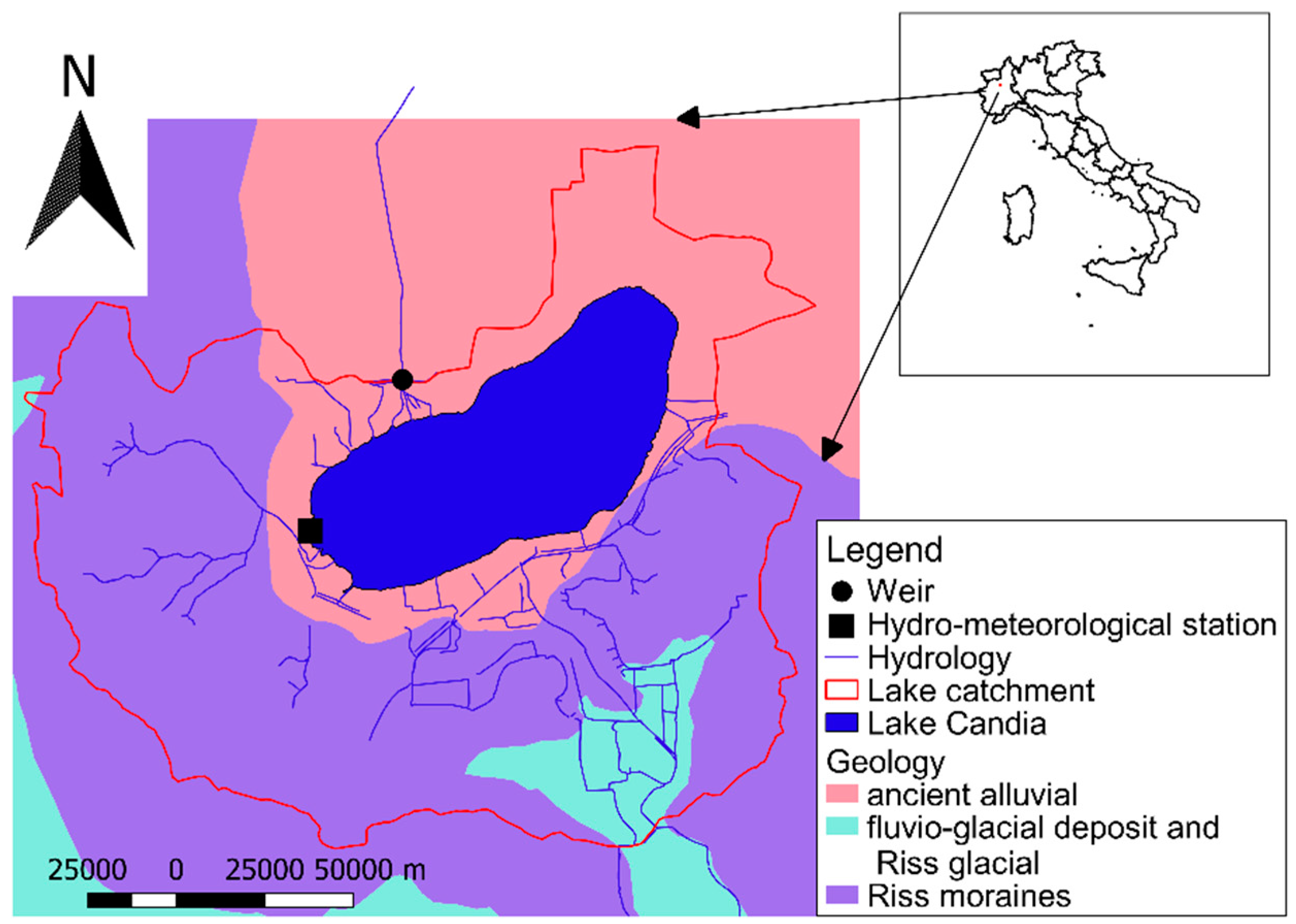
Lake Candia (Figure 1) is the second largest lake of the IMA and it is likely fed primarily by groundwater and rainwater, rather than by the small canals running along the surrounding hillslopes. A small outlet links the lake to the Dora Baltea River. Water exchange is slow and the concentration of nutrients is consequently high, due to the runoff from the surrounding agricultural fields and to the natural lake conditions. Since 1995, the lake and the wetlands have been protected as a natural reserve, the first provincial park in Italy. Furthermore, the park was declared a site of community importance according to the European Union “Habitat” directive. Lake Candia will also soon be included in the list of protected wetlands, according to the Ramsar Convention (http://www.parks.it/parco.lago.candia/Eindex.php, accessed date: 2 November 2021). The definition of adequate water management strategies for these particular ecosystems, taking into account the impact of climate change on these lakes, can offer tools for the protection of ecosystems and recommendations for sustainable development. The Lake Candia watershed covers 8.91 km2 and has a mean altitude of 266 m a.s.l. Maximum depth of the lake is 7.7 m, average depth is 4.7 m, and volume is 0.007 km3.
The Lake Candia catchment is characterized by intense agricultural land use, where the arable portion is the largest. The surplus water of the agricultural network is discharged directly into the lake. The lake is fed primarily by groundwater and by rainwater falling directly on its surface; runoff from the watershed is the third source in order of importance, with characteristics varying according to the amount of rainfall and the season [17]. The lake’s outflow, the Fosso Traversaro, with which the watershed comes to an end, is in the southwestern part of the lake, off-center from the more northerly orientation of the lake. The discharge is regulated by a weir (Figure 1).
Following Köppen’s classification [18], the lake area has a temperate sub-continental climate, with daily average air temperatures ranging from −2 °C in the coldest month (January) to 30 °C in the hottest (July). The rainfall regime is western sub-littoral, according to the climate classification reported by [18], and is characterized by two maxima and two minima, with the highest maximum in spring and the lowest minimum in winter, with mean annual values around 900 mm.
Some equipment was installed in 1987 on the southwestern shore of Lake Candia (Figure 1) to measure the main meteorological parameters, such as rainfall, air temperature, wind direction and speed, solar radiation (direct and reflected), humidity, pressure, and lake level. In April 1987, a trapezoidal Cipoletti weir was built at the outlet (Figure 1) to regulate the discharge so that water would not flow out of the lake if the water level fell below 30 cm. The data from the weather station available for climate analyses are recorded continuously; the station is operated by the Regional Protection Agency (ARPA) of Piedmont Region (http://www.arpa.piemonte.it/rischinaturali/accesso-ai-dati/annali_meteoidrologici/annali-meteo-idro/banca-dati-meteorologica.html, accessed date: 2 November 2021). The weir discharge data are in direct relation with the level of the lake, so that a continuous reading of the levels gives a continuous discharge datum for the outflow.
The analyses were carried out using meteorological and discharge data recorded at the automatic measuring station and were used for: (i) evaluating water balance to determine the amount of groundwater; (ii) evaluating the trend of each component of water balance (rainfall direct on lake; entrance, the component that comprises runoff, exceeded irrigation, and irrigation runoff; groundwater; discharge from the emissary; and volume variation); (iii) calculating the presence of break point or changes in the behavior of each component; and (iv) investigating the regression of water balance terms to understand their relationship, including possible effects among each other and for improvement of water research management.
2.1. Water Balance
Using monthly data from 1993 to 2019, a two-step approach was used to calculate the volume of groundwater and thus evaluate its importance in the Lake Candia hydrological regime. As the study area contains a water body (Lake Candia), which exercises its hydraulic action on the magnitudes of the water balance terms, the continuity equation was applied first to the lake and then to the whole basin.
The continuity equation applied to the lake follows:
where:
- PLC
- is direct rainfall on the lake surface and on the part of the reed bed connected to it;
- RS
- is the surface runoff;
- IRE
- is the portion of irrigation water that is not used and enters the lake directly;
- RIR
- is the runoff from irrigation;
- QS
- is the underground contribution of groundwater via resurgences plus hyporheic groundwater flow;
- ELC
- is the evaporation from the lake and evapotranspiration from the reed bed;
- ΔH
- is the variation in the level of the lake, taken with its sign;
- Q
- is the surface discharge measured at the outlet of the lake.
If we look at the whole equation [20], the water entering the lake is made up of total rainfall P, transformed into rainfall on the lake (PLC) and net rainfall (RS); irrigation water, which must be taken into account due to the presence of a number of cultivated fields, and a further addition from groundwater (QS), which is thought to feed the lake due to the existence of resurgences within the lake and the hyporheic flow [21]. With respect to the general equation, the outgoing water comprises the evaporation of both water body and reed bed (ELC); variations in the level of the lake (ΔH), taken as increases and reductions of its volume; and the discharge measured at the weir (Q) located on the outlet. At this initial stage, neither evapotranspiration from vegetation in the watershed nor variations in soil moisture content have been taken into account.
The criteria adopted to obtain each of the terms of the balance are given below.
- PLC—Rain falling directly on the lake and the reed bed.
This is the portion of precipitation falling directly on the lake and the reed bed, most of which grows with its roots in the lake or floating [22], thus without being intercepted by plants or soil. It was calculated by multiplying the rainfall depth by the lake area and the reed bed area.
- RS—Surface runoff
This portion of precipitation is also called net rainfall or surface discharge, or the rainfall to the soil that is not infiltrated but reaches the lake directly through surface runoff. RS was calculated using the United States Soil Conservation Service curve number method for the study of small rural watersheds [23].
According to this method, the surface discharge is a function of precipitation P and a parameter S, which represents the quantity of water that can be stored in the watershed (or in the terrain). The parameter S is a function of the infiltration capacity (characterized by the minimum infiltration rate observed in soil without vegetation after a long wet period), the totality of the conditions (soil use, surface treatment, drainage), and the soil moisture content (or antecedent moisture condition, AMC). The parameter S is linked to another, non-dimensional parameter called runoff curve number, or simply curve number, CN. The CN value is determined using two different tables, one developed for agricultural and wooded areas [24] and the other for urban and kindred areas [25].
Considering the type of soil cover, use, and class, and the CN values for each category, we calculated the surface runoff for the watershed of Lake Candia. A reduction of 20% was applied in the category BUILT-UP AREAS and 50% in the category STREETS/ROADS to the net rainfall value obtained using the CN method [23] considering that a portion of rainfall in built-up areas and streets can be intercepted by grassland, vegetation, or drainage system through, for example, manholes [25].
- IRE—Excess irrigation water
This is unused irrigation water that is channeled directly into the lake. According to the irrigation consortium, the period for irrigation is between 15 May and 15 September for 30 h/week with a volume of water around 0.027 m3 × 106 per year. The water extraction is 160 L/s.
- RIR—Irrigation runoff
This parameter was calculated with the same method used for runoff from rainfall, after transforming into mm of rainfall the quantity of irrigation water derived from outside the basin and distributed weekly over the whole irrigated area from 15 May to 15 September. In calculating the runoff, only the irrigated surfaces within a band of about 200 m from the lake shores were taken into consideration, as it was thought that the water used farther away would all be absorbed by the soil. The size of this parameter was taken as the same for every year of the study, and equivalent to 0.005 m3 × 106.
- QS—Underground contribution
This contribution is an unknown quantity in the balance. It is calculated by Equation (1) in this form:
- ELC—Evaporation from the lake and evapotranspiration from the reed bed
Evaporation from the lake (or from the free water) was calculated using the energy balance method which hypothesizes a regime in which the net solar radiation absorbed by the water for a certain period of time is partly released as sensible heat to land and air in contact with the water, and partly used to transform the water into vapor [26]. The calculation was performed using temperature, global solar radiation, and reflected solar radiation data, measured at the Candia meteorological station. As we mentioned above, the reed bed grows on the lake and is always saturated with water, so that its evapotranspiration is linked to the evaporation of the lake. The ETC (evapotranspiration of the reed bed) was thus given an equal value to that of the lake evaporation multiplied by 1.7 in the months when the reed bed is growing, i.e., June, July, August, and September, and exactly equal to the evaporation from the lake in the other months of the year when it is not growing [27]. The two values obtained, multiplied by the relative area covered by the reed bed, were added and included into the balance equation together.
- ΔH—Variations in the lake level
The daily variations in the level of the lake, obtained from the values registered by the water gauge of Candia, were calculated to obtain the actual monthly variation of the lake volume. The variation is taken with its sign, i.e., if the level falls, there will be a corresponding decrease in the volume and the value will be negative, while an increase in volume is calculated as positive.
- Q—Surface discharge (outflow)
The last term in the balance Equation (2) is the discharge at the outlet, i.e., the quantity of water exiting the lake. The discharge is measured using the weir at the closing section of the lake that regulates its activity, and is connected with the levels of the lake that are continuously measured through the equation.
By inserting each term of the balance in the Equation (2), we could obtain the value of the monthly and annual underground contribution for different years, from 1993 to 2019. The underground contribution thus obtained takes account both the contribution of groundwater via resurgences and any hyporheic flow of infiltration water returning to the lake underground. These two contributions must be separated if we want to estimate only the groundwater source. Thus, to identify the groundwater source it is necessary to use a general hydrological balance equation, applied not only on the lake but on the whole catchment, so we consider a control volume represented by a volume that has the base coinciding with the waterproof layer of the aquifers and the upper limit above the vegetation; the general equation of water balance follows:
where
P = ET + Q + ΔV
- P
- is the precipitation on the whole control volume;
- ET
- is the evapotranspiration of the vegetation within the control volume;
- Q
- is the water flux in and out of the whole control volume;
- ΔV
- is the volume stored within the whole control volume.
Thus, using the general balance equation [20], which also includes evapotranspiration and the quantity of infiltrated water, and applying Thornthwaite’s method for determining the annual soil water cycle, we defined the portion of hypodermic discharge, which allowed us to determine the effective contribution of groundwater source to the lake:
where
- GS
- is the groundwater source;
- QS
- is the underground contribution of groundwater via resurgences plus hyporheic groundwater flow;
- Di
- is the hyporheic groundwater flow;
- Q
- is the surface discharge measured at the outlet of the lake;
- ELC
- is the evaporation from the lake and evapotranspiration from the reed bed;
- RS
- is the surface runoff, i.e., the rainfall that reaches the lake directly from the surrounding terrain;
- IRE
- is the portion of irrigation water that is not used and enters the lake directly;
- ΔV
- is the variation in the volume of the lake, taken with its sign;
- PLC
- is direct rainfall on the lake surface and on the part of the reed bed connected to it;
- RIR
- is the runoff from irrigation, i.e., the part of irrigation water that is not absorbed either by plants or the soil and reaches the lake directly;
- IR
- is the irrigation within the catchment;
- ET
- is the evapotranspiration of vegetation within the whole catchment calculated with the Thornthwaite’s method:where
- ETp
- is the monthly potential evapotranspiration (in cm) relative to a 30-day month and with duration of insolation of 12 out of 24 h;
- is the monthly average temperature in °C;
- K
- is the coefficient of the irradiation of the month, obtained by:where
- N
- is the observed maximum number of sunny hours for a day, divided by its maximum expected number depending on the latitude, in our case, 12;
- d
- is the number of day per month, divided by the average number of day per month;
- I
- is the annual heat index, sum of the monthly heat index [28];
- a
- is a coefficient function of I and the latitude [28].
Thornthwaite suggested a method for the simulation of the hydrological phenomenon in a catchment to evaluate the agricultural deficiency (calculated as the difference of the water need ETp and the actual crop ET), which is based on a formula of evaporation of a generic crop [29]. The evaluation of evapotranspiration is necessary for agricultural issues and, especially, for the definition of water resource balance [30]. Another method used to evaluate evapotranspiration is Penman–Monteith method [31], considered more physically realistic but requiring many meteorological variables. The Thornthwaite method is more easily applied because it requires only monthly mean air temperature and the maximum amount of sunshine duration, calculated using latitude [32,33]. The results obtained through these two methods are very similar in terms of correlation, trend, and regional averages [32,33]. First, the potential evapotranspiration is calculated with the aforementioned formula, and then the actual evapotranspiration is calculated using the Turc formula [23].
If the monthly rainfall is more than the potential evapotranspiration, the actual evapotranspiration is considered equal to its potential; the rainfall surplus is assigned to the soil humidity until an assigned limit [20]. The possible precipitation remaining is assigned to the runoff and to the groundwater flow, with the criterion explained below. If the monthly rainfall is less than the potential evapotranspiration, the actual evapotranspiration is considered equal to the total rainfall plus the soil humidity; if the supply is sufficient, the actual evapotranspiration is equal to its potential value, otherwise it is equal to the sum of the precipitation and the water storage such as soil humidity. The water excess that is not lost by evapotranspiration or stored in the soil humidity is assigned half between the monthly runoff in which there is the excess and half in the following month (underground flow) [34].
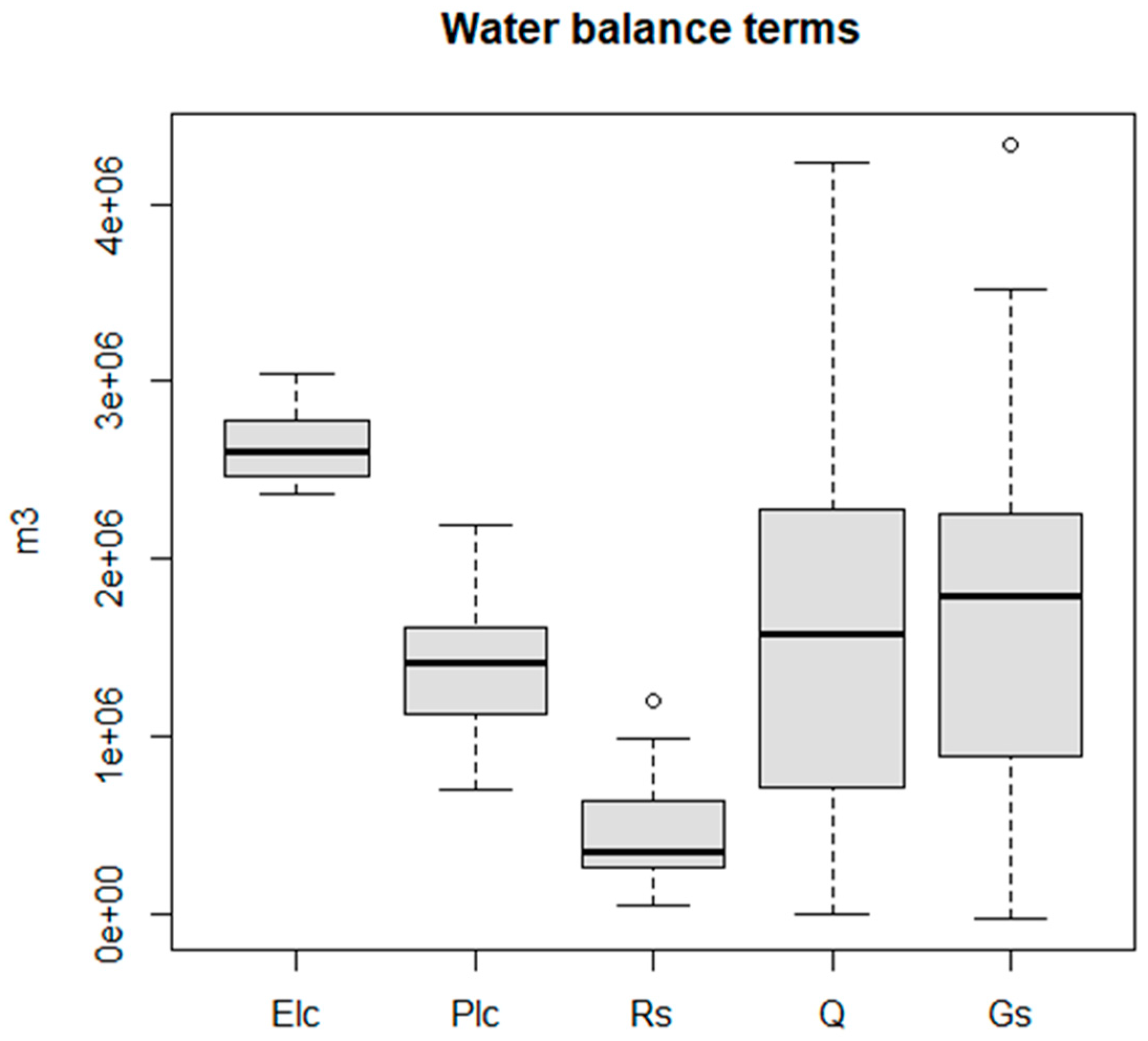
The main parameters of the hydrological balance are represented using a box plot that allows for understanding if the distribution is symmetric or asymmetric, and to identify the presence of outliers.
These anomalous values were calculated using Tukey fences: the lower threshold equal to Q1 − 1.5 ∗ IQR and the upper threshold equal to Q3 + 1.5 ∗ IQR, where Q1 is the lower quartile, Q3 is the upper quartile, and IQR is the interquartile range.
2.2. Trend of Each Component of Water Balance
Monthly time series of the main component of water balance, such as direct rainfall on lake (PL), the sum of all surface water inflow into the lake (E = RS + RIR + IRE), the variation of lake volume (ΔV), the lake level (H), the outflow (Q), and the groundwater source (GS) were analysed for the period from 1993 to 2019 using R software, version 3.6.3 [35]. Decomposition of each water balance component of the time series into its constituting parts, namely, the observed trend, seasonality, and random parts, was done for the monthly time series from 1993 to 2019 using the time series functions in R. The observed part represents the data that were measured or calculated through water balance; the trend part specifies if there is an increase or a decrease around the mean value; the seasonal part represents a cyclical trend; and the random part represents unpredictable changes in the data without a precise and identifiable cause.
Deseasonality was performed to correctly identify an increasing or decreasing trend in water balance component and then subtract the seasonal component from the original time series. Statistical tests to verify the trends and assess their significance were performed using the Mann–Kendall test [36,37]. This test was selected because of its lower sensitivity to outliers and its robustness for detecting a trend in rainfall, temperature, and hydrology, without specifying if the trend is linear or nonlinear [38,39]. In addition, this test identifies a monotonic trend that defines an increasing or decreasing trend, is simple and robust, and adapts to missing values and data that do not have any particular distribution for improving water resource management, detecting a trend in discharge, direct runoff, precipitation, and evaporation [40,41].
2.3. Break Point
The statistical problem of break point or tipping point in a trend has been addressed in many fields of research, such as medical, images analyses, and human activity [42] but especially on meteorological and climate parameters [43], hydro-meteorological variables [44], and on time series data [45]. Methods in change detection or change point detection in time series data try to identify the times when the probability distribution of a stochastic process such as a time series changes.
Detection of break points, in this study, was done using the algorithm of analyses on change point present in the R library strucchange [46,47] applied to water balance parameters seasonally adjusted in the previous step. The approach we followed was to use least squares regression to estimate the locations of the changes. The function selects an optimal model (choosing the number of change points) using the Bayesian information criterion (BIC) by default [48]. The assessment of changing point was carried out by checking the changes in the average and variance of each variable of water balance, returning the point in time, year or month, in which one or more turning points were highlighted. Furthermore, recent studies in Piedmont Region where Lake Candia is located, highlight a break point in the water table level in 2008, due to a different agricultural technique of rice cultivation; the dry direct-seeded rice technique replaced the traditional techniques in some areas of the Piedmont Plain, affecting water use in the study area [49]. It is therefore interesting and useful to verify any climate break point, to compare with the changes in groundwater level and analyze the trend and behavior of meteorological data before and after 2008.
2.4. Understanding the Drivers of Water Balance
After investigating the trend of main water balance terms and looking for potential break points, we wanted to evaluate the relative importance of each term (ΔV, PL, Q, GS, E) to determine the main driver of water resource management of Lake Candia. We considered that PL is the direct rainfall on the lake and represents an important entrance that depends only on meteorological factors; Q is the discharge of the outflow and depends on the form of the weir placed on the outflow; GS is the groundwater entrance and depends on the rainfall within the whole hydrogeological catchment and on the water use (water supply and agricultural); E is the other surface entrance, depending on rainfall, land use, and irrigation; ΔV is the variation of the lake volume that depends on rainfall, discharge, runoff, and groundwater supply. The variation of lake level (ΔH) is incorporated into the ΔV term.
Then to avoid various types of noise (e.g., small sample efficiency, outliers, high breakdown point, time complexity) we adopted robust linear regression [50,51] LTS, with the lqs package, Huber function, and bisquare estimate using the R package MASS [52] for Formula (3).
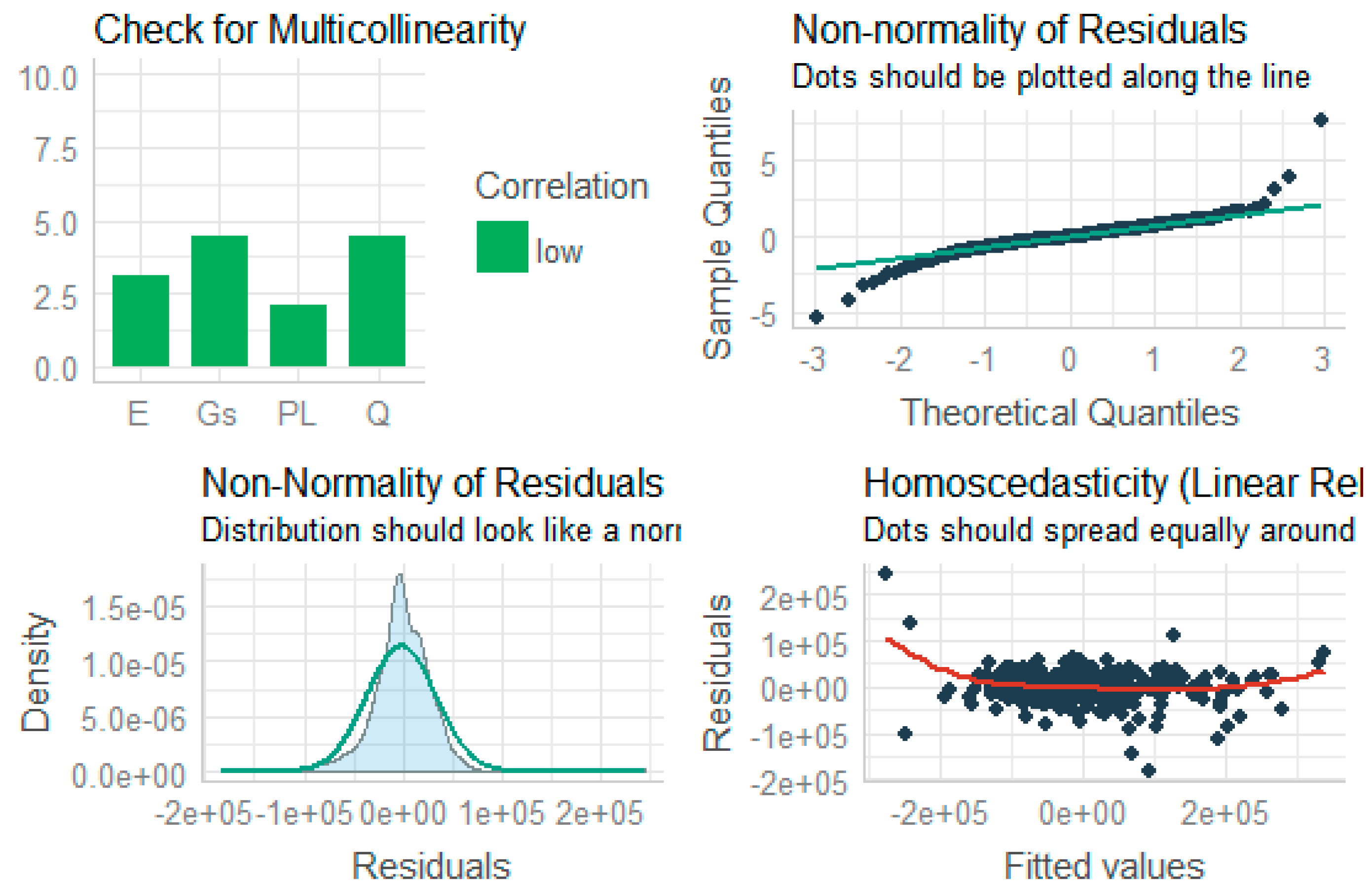
In any multiple regression analysis, it is necessary to highlight multicollinearity, recognizing regressor variables affected by linear dependencies [53], because this issue may cause serious complication with the reliability of the regression parameter evaluation [54]. The selection of predictors depends on many factors and particular attention must be given; nevertheless, it happens that standard error of the coefficient will increase or that some statistically insignificant variables should be significant; this is due to multicollinearity [55]. In cases of pairs of predictors with Spearman correlation values greater than 0.8, only one predictor was kept. The R package performance [56] was then used to check regression model fit, to its defined quality and goodness, and to check the model’s various assumptions (i.e., normality of residuals, normality of random effects, heteroscedasticity, homogeneity of variance, and multicollinearity), and that it includes R2, root mean squared error (RMSE), and intraclass correlation coefficient (ICC) [56].
Finally, we assessed the relative importance of an individual regressor’s contribution to the multiple regression model in explaining ΔV by using the R package relaimpo [57].
3. Results
3.1. Water Balance
The box plot (Figure 2) shows the distribution of the main water balance terms, their symmetry, and the presence of outliers. The outflow (Q) and the groundwater contribution (GS) have a higher variability than the other terms considering the distance between the quartiles. Moreover, runoff (RS) and the groundwater contribution (GS) highlight the presence of outliers.
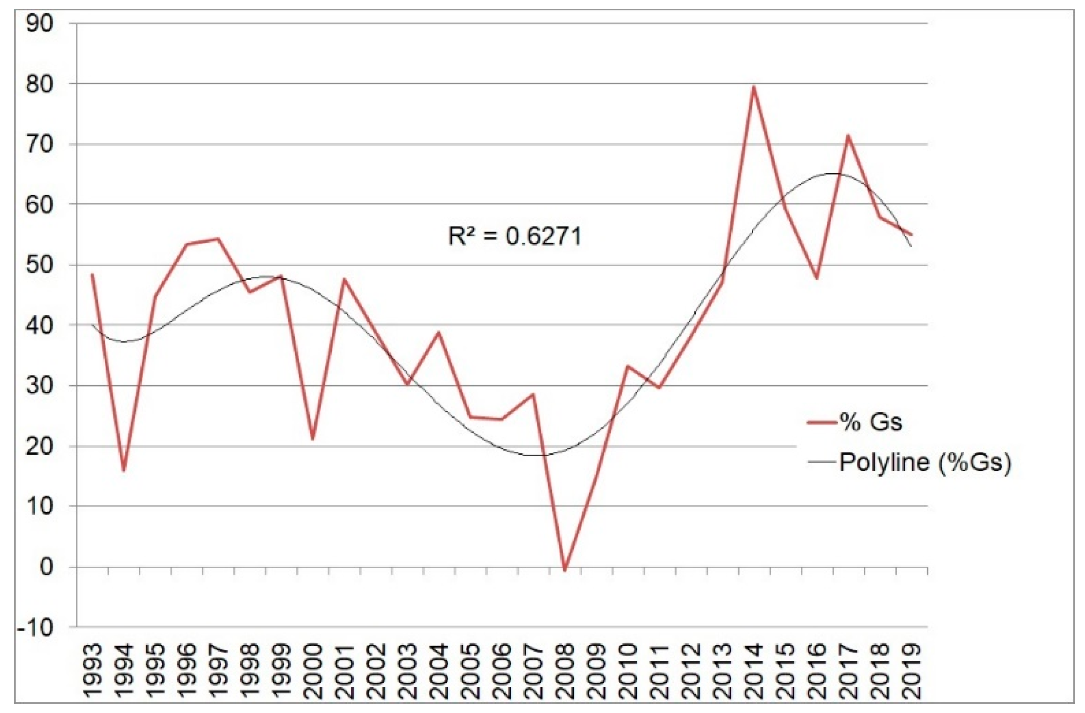
The mean contribution of the groundwater source is around 41% of the entrance of the hydrological balance, with a minimum around −1% and a maximum around 79%. From the annual water balance analyses, we can highlight the negative contribution of the groundwater resource in 2008.
The tendency of percentage of groundwater (%Gs) is reported in Figure 3. The tendency was an increase starting in 2008 and a decrease starting in 2014.
3.2. Trend of Each Component of Water Balance
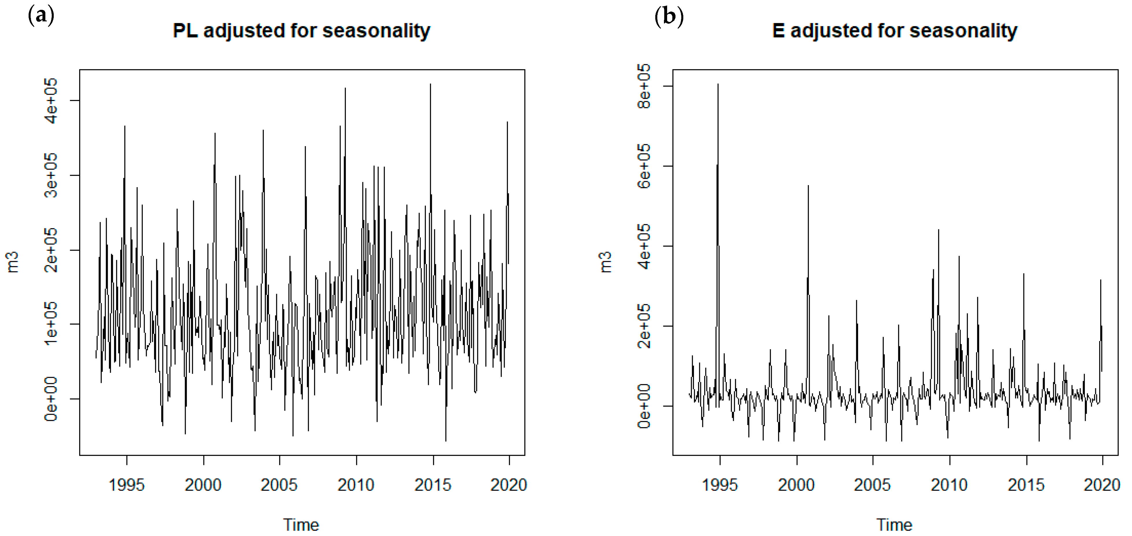
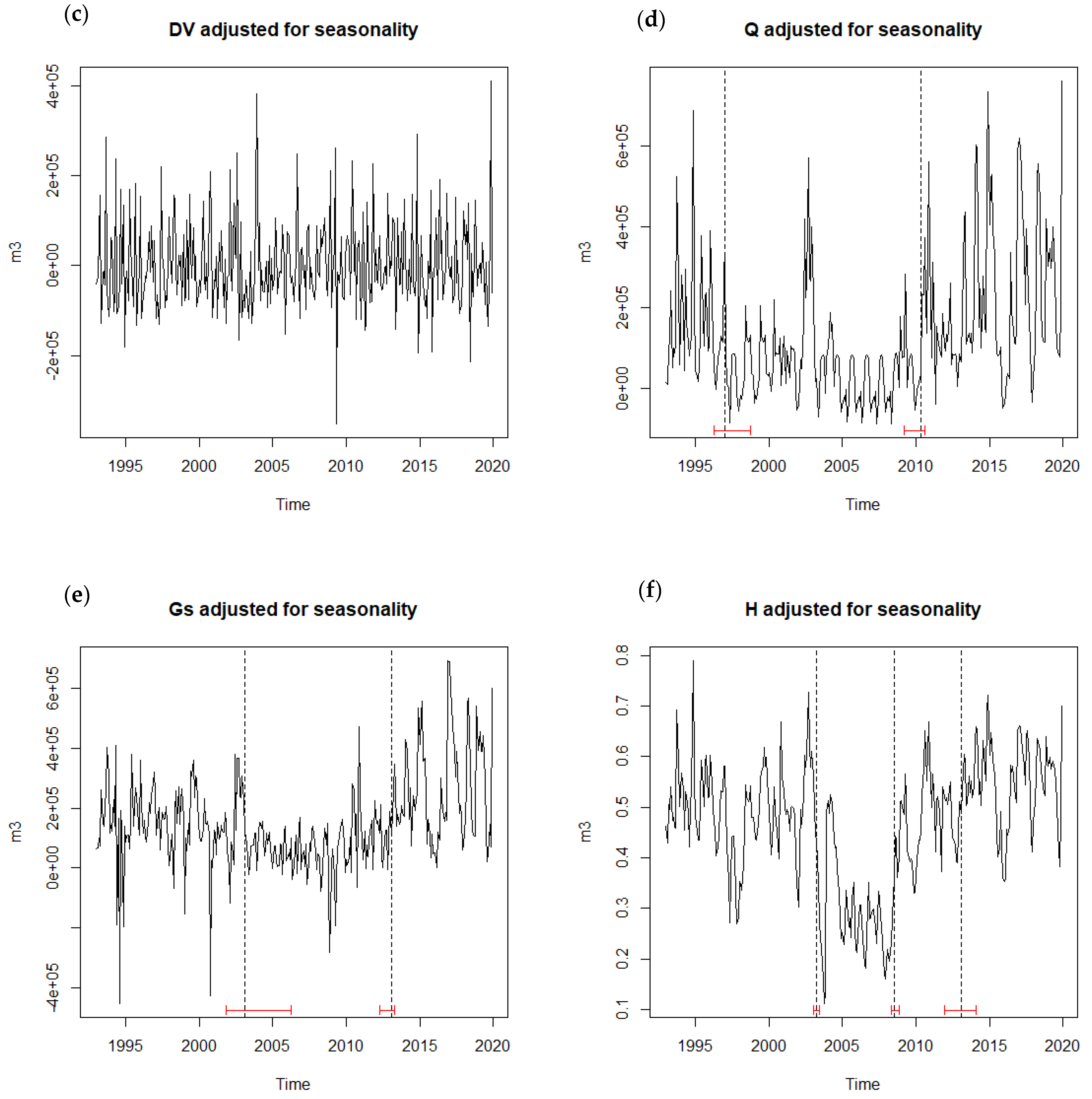
Analyzing the trend part of the time series for each term of the water balance, only the outflow (Q), lake level (H), and the groundwater source (GS) seem to have a clear trend from around 2010, whereas rainfall (PL), water inflow (E), and the lake volume variation (ΔV) seem to fluctuate around the average with no trend (Figure 4). Therefore, subtracting the seasonal component from the original time series (Figure 4), the time series adjusted for seasonality supported that only outflow (Q), lake level (H), and groundwater (GS) had a significant trend (Table 1).
3.3. Break Point
As already highlighted in the analysis of trends in the time series, not all of the terms analyzed for the assessment of the hydrological balance of Lake Candia revealed trends. The additional tests to identify break points verified that there were no significant changes in the volume variation of the lake (ΔV) and no turning points in the rainfall (PL) and in the overall lake water inflow (E) (Table 2 and Figure 4). Groundwater (GS), lake level (H), and surface discharge at the outlet (Q) revealed significant breaks (Table 2 and Figure 4); two of the timing of changes for GS and H overlap in 2003 and 2013. Only H seems to be affected by the change in different cultivation of rice, with a break point in 2008.
3.4. Drivers of Water Balance
The first estimate on the correlation among different predictors is reported in Figure 5; QS (underground component of the groundwater term) has a high correlation value (0.88) with only GS (groundwater source) retained in the regression model.
No multicollinearity was found by using the performance model, and non-normality of residual and homoscedasticity was not a problem (Figure 6).
The robust linear regression model comparing lqs (method = “lqs” and “lts”), and rlm (method = psi.huber, psi.bisquare) suggested that the most appropriate model was rlm with Huber psi. Model check supported the reliability of model fit.
The selected model of robust regression (Table 3) provides the formula:
ΔV = 0.77PL − 0.37Q + 0.30GS + 0.52E − 103820.06
The analyses of the relative importance of the four regressors indicates that direct rainfall on lake (PL) has more importance than the other regressors with R2 equal to 0.58 and the groundwater sources (GS) has the lowest R2 value, equal to 0.05.
4. Discussion
The analyses conducted on the complex hydrogeological system that characterizes Lake Candia show that the direct rainfall on lake (PL) and the entrances (E) to lake as, for example, runoff, have an importance greater than the groundwater resource (GS), even if a reliable inference was not possible without further validation and in situ measurements [6]. Groundwater seems to have less importance than surface water entrance on lake level variation, probably because the exchange between groundwater and lake water is slow, even when prolonged in time. Direct rainfall and runoff have more impact on lake level because they carry more water in a short time. With direct measurement of groundwater, it would be possible to define which inflow determines the permanence of a certain level in the lake rather than that its high variation, thus defining the actual importance of groundwater. The response of groundwater source to rainfall was highly variable in our system and it is known that it depends on physical characteristics of soil and aquifer, size of lakes, and their catchments [58,59]. The analyses of the main water balance components during the period 1993–2019 revealed that only the outflow, the groundwater source, and the lake level had a significance and positive trend. The variability in rainfall, water inflow, and the consequent variability in lake volume were likely too high, masking potential temporal trends.
The analyses on break points, to verify if water balance components could change their behavior in particular circumstance or for particular events, revealed that no changes could be detected for water inflow and for volume variation, probably due to the high variability of their behavior and to the variables that affect them. Rainfall varies greatly through time and no trend or changing points were identified. Entrance has a behavior depending on rainfall and on agricultural need, which depend, in turn, on temperature and cultivation. Lake volume is more stable and for this reason its behavior is not subject to particular trend or change points. Break points in the outflow were found in 1997 and 2010; in the groundwater source in 2003 and 2013 but not in 2008; and in the lake level in 2003, 2008, and 2013. Regarding the outflow, the two years detected as changing points are linked with an unexpected decrease (in 1997) in comparison to previous years, and with an increase (in 2010) after a series of years with low values.
Between 2003 and 2008, lake levels were characterized by low values whereas since 2008 and even more since 2013, an increase of their values occurred. Probably the flooding of the marsh (located in the northeastern part of the lake) during 2008–2009 by a LIFE project (http://www.life.trelaghi.it/eng/tasks5.htm, accessed date 2 November 2021) increased minimum lake level, in addition to allowing more water quantity into the lake catchment. This greater water quantity since 2013 was also pointed out by a groundwater source break point, which showed an increase of groundwater. This increase is in contrast with [49], who considered a reduction in groundwater source because of changes in water use owing to increasing cultivation, but it is in line with unpublished results of a study on Lake Viverone, from the same morainic amphitheater, showing an increase of groundwater level since 2008 measured from a well into the catchment of the lake. An explanation for the increase could be related to a greater contribution by the alpine glaciers from which it is fed, due to warmer and longer summers melting more glacial mass [60,61].
The evaluation of temporal variability of different climatic variables related to climate change is surely relevant for water resource management, to allow knowledge-based planning uses and to understand the effect of human disturbance, and the application of break point detection can be a key tool to achieve the goal [43]. Yet, the problem of break point is not often included in climate change studies, which are more interested on the magnitude of changes in temperature, rainfall, or solar radiation, instead of detecting when such changes occurred. The field of analysis of sudden changes and tipping points in the behavior of environmental variables represents a rising scenario in ecological studies [62,63] and will surely provide new insights in the understanding of the effects of climate change.
To better understand relationships among the different components of water balance, the regression analysis provides a model that can be used to improve water management.
The groundwater resource can be followed by monitoring water table levels, and management policies implemented to respond in advance to changes in water table considering that it is the most important reservoir of the Piedmont Region [64]. Furthermore, the preservation groundwater quantity and quality are extremely important topics to protect groundwater from pollution and exploitation [65]. Such an approach, combining management of outfall and water table monitoring, can be adopted for the protection of the water resource together with the sustainable uses and protection of the ecosystem of Lake Candia. Rainfall is a meteorological parameter, which has direct influence on agricultural production and on water resources and water availability; a decrease in rainfall will prompt greater extraction of groundwater for irrigation and will result in a decline of groundwater level, with consequences on water balance. The scenario of changing water availability in the future needs to be properly taken into account for long-term water management at the catchment scale [41], as needed for Lake Candia.
5. Conclusions
The water balance of Lake Candia revealed a very important influence of direct rainfall on the lake and subsequently of different typologies of entrance (runoff from rainfall and irrigation), whereas the groundwater resource seems to have minor importance even if with a significant increasing trend of its importance. Although the variation of lake volume was affected by direct rainfall and surface water inflow, the effect of groundwater has to be carefully considered to support predictive management of the water resource.
The relationship between meteorological variables and the hydrogeological cycle are clear and their trends also known. On the contrary, the actual trends in groundwater are difficult to determine, especially regarding quantities and timing of events, particularly in the absence of measures of permeability, porosity, storage coefficient, and the effective value of exchanges between the different aquifers present in the catchment. Furthermore, the fact that the territory surrounding the lake is used for agriculture increases the need for surface water and groundwater. For these reasons, a more detailed evaluation of the dynamics of the groundwater is a priority, both for the correct management of water resources in general, and for greater protection of the Lake Candia ecosystem.
Author Contributions
Conceptualization, M.C., C.D. and H.S.; methodology, M.C. and H.S.; software, M.C.; validation, M.C., C.D. and H.S.; formal analysis, M.C.; investigation, M.C.; data curation, M.C. and C.D.; writing—original draft preparation, M.C.; writing—review and editing, C.D. and H.S.; visualization, M.C., C.D. and H.S.; supervision, M.C. All authors have read and agreed to the published version of the manuscript.
Funding
This research received no external funding.
Data Availability Statement
Data used for the analyses are available at the following links: http://www.arpa.piemonte.it/rischinaturali/accesso-ai-dati/annali_meteoidrologici/annali-meteo-idro/banca-dati-meteorologica.html, http://www.arpa.piemonte.it/rischinaturali/accesso-ai-dati/annali_meteoidrologici/annali-meteo-idro/banca-dati-idrologica.html, accessed date 2 November 2021.
Acknowledgments
The authors thank the anonymous reviewers and the editor for their useful comments, which substantially improved the manuscript.
Conflicts of Interest
The authors declare no conflict of interest.
Abbreviations
| IMA | Ivrea Morainic Amphitheatre |
| ARPA | Regional Protection Agency |
| AMC | Antecedent Moisture Condition |
| CN | Curve Number |
| ETC | Evapotranspiration of the reed bed |
| IQR | Interquartile Range. |
| BIC | Bayesian Information Criterion |
| LTS | Least-Trimmed Squares |
| RMSE | Root Mean Squared Error |
| ICC | Intraclass Correlation Coefficient |
References
- Jasrotia, A.S.; Majhi, A.; Singh, S. Water balance approach for rainwater harvesting using remote sensing and GIS techniques, Jammu Himalaya, India. Water Resour. Manag. 2009, 23, 3035–3055. [Google Scholar] [CrossRef]
- Kendy, E.; Gérard-Marchant, P.; Todd Walter, M.; Zhang, Y.; Liu, C.; Steenhuis, T.S. A soil-water-balance approach to quantify groundwater recharge from irrigated cropland in the North China Plain. Hydrol. Proces. 2003, 17, 2011–2031. [Google Scholar] [CrossRef]
- Xu, C.Y.; Singh, V.P. Evaluation of three complementary relationship evapotranspiration models by water balance approach to estimate actual regional evapotranspiration in different climatic regions. J. Hydrol. 2005, 308, 105–121. [Google Scholar] [CrossRef]
- Winter, T.C. Uncertainties in estimating the water balance of lakes. J. Am. Water Resour. Assoc. 1981, 17, 82–115. [Google Scholar] [CrossRef]
- Kishel, H.F.; Gerla, P.J. Characteristics of preferential flow and groundwater discharge to Shingobee Lake, Minnesota, USA. Hydrol. Process. 2002, 16, 1921–1934. [Google Scholar] [CrossRef]
- Rudnick, S.; Lewandowski, J.; Nützmann, G. Investigating groundwater-lake interactions by hydraulic heads and a water balance. Groundwater 2015, 53, 227–237. [Google Scholar] [CrossRef] [PubMed]
- Scheffer, M.; Jeppesen, E. Regime shifts in shallow lakes. Ecosystems 2007, 10, 1–3. [Google Scholar] [CrossRef] [Green Version]
- Scheffer, M.; Hosper, S.H.; Meijer, M.L.; Moss, B.; Jeppesen, E. Alternative equilibria in shallow lakes. Trends Ecol. Evol. 1993, 8, 275–279. [Google Scholar] [CrossRef]
- Nisbeth, C.S.; Jessen, S.; Bennike, O.; Kidmose, J.; Reitzel, K. Role of groundwater-borne geogenic phosphorus for the internal P release in shallow lakes. Water 2019, 11, 1783. [Google Scholar] [CrossRef] [Green Version]
- Mavromatis, T.; Stathis, D. Response of the water balance in Greece to temperature and precipitation trends. Theor. Appl. Clim. 2011, 104, 13–24. [Google Scholar] [CrossRef]
- Coops, H.; Beklioglu, M.; Crisman, T.L. The role of water-level fluctuations in shallow lake ecosystems–workshop conclusions. Hydrobiologia 2003, 506, 23–27. [Google Scholar] [CrossRef]
- Colombero, C.; Comina, C.; Gianotti, F.; Sambuelli, L. Waterborne and on-land electrical surveys to suggest the geological evolution of a glacial lake in NW Italy. J. Appl. Geophys. 2014, 105, 191–202. [Google Scholar] [CrossRef] [Green Version]
- Laghari, A.N.; Vanham, D.; Rauch, W. The Indus basin in the framework of current and future water resources management. Hydrol. Earth Syst. Sci. 2012, 16, 1063–1083. [Google Scholar] [CrossRef] [Green Version]
- Ruffino, B.; Fiore, S.; Genon, G.; Cedrino, A.; Giacosa, D.; Bocina, G.; Fungi, M.; Meucci, L. Long-term monitoring of a lagooning basin as pretreatment facility for a WTP: Effect on water quality and description of hydrological and biological cycles using chemometric approaches. Water Air Soil Pollut. 2015, 226, 331–343. [Google Scholar] [CrossRef]
- Gianotti, F.; Forno, M.G.; Ivy-Ochs, S.; Monegato, G.; Pini, R.; Ravazzi, C. Stratigraphy of the Ivrea Morainic Ampitheateatre (NW Italy): An updated synthesis. Alp. Mediterr. Quat. 2015, 28, 29–51. [Google Scholar]
- Lucchesi, S.; Gianotti, F.; Giardino, M. The morainic amphitheatre environment: A geosite to rediscover the geological and cultural heritage in the examples of the Ivrea and Rivoli-Avigliana morainic amphitheatres (NW Italy). In Engineering Geology for Society and Territory; Springer: Cham, Switzerland, 2015; Volume 8, pp. 245–248. [Google Scholar]
- Ciampittiello, M.; de Bernardi, R.; Galanti, G.; Giussani, G.; Cerutti, I.; Salerno, F.; Tartari, G. Definizione degli Ambiti Idrografici e Idrogeologici dei Bacini Oggetto dello Studio: Lago di Candia. Progetto MI.CA.RI. Strumenti e Procedure per il Miglioramento della Capacità Ricettiva di Corpi Idrici Superficiali; Report CNR-ISE. 2004, p. 18. Available online: http://www.vb.irsa.cnr.it/images/seminar/Report/Report_2004_01_Micari_pr.pdf (accessed on 2 November 2021).
- Fratianni, S.; Acquaotta, F. The climate of Italy. In Landscapes and Landforms of Italy; Springer: Cham, Switzerland, 2017; pp. 29–38. [Google Scholar]
- Sambuelli, L.; Bava, S. Case study: A GPR survey on a morainic lake in northern Italy for bathymetry, water volume and sediment characterization. J. Appl. Geophys. 2012, 81, 48–56. [Google Scholar] [CrossRef] [Green Version]
- Thornthwaite, C.W.; Mather, J.R. Instruction and tables for computing potential evapotranspiration and the water balance. In Climatology; Centerton: New Jersey, NJ, USA, 1957; Volume 10. [Google Scholar]
- Sambuelli, L.; Comina, C.; Bava, S.; Piatti, C. Magnetic, electrical, and GPR waterborne surveys of moraine deposits beneath a lake: A case history from Turin, Italy. Geophysics 2011, 76, 1–12. [Google Scholar] [CrossRef] [Green Version]
- Topa, E.A. Ecologia Della Comunità Macrofitica Emersa del Lago di Candia. Ph.D. Thesis, University of Milan, Milan, Italy, 1991. (In Italian). [Google Scholar]
- Moisiello, U. Idrologia Tecnica; La Goliardica Pavese: Pavia, Italy, 1999; p. 824. [Google Scholar]
- SCS (Soil Conservation Service) Hydrology. In National Engeneering Handbook; Water Resource Publication: Littleton, CO, USA, 1985; Section 4.
- SCS (Soil Conservation Service) Urban Hydrology for Small Watersheds; Technical Release 55; U.S. Department of Agriculture: Washington, DC, USA, 1975.
- Chow, V.T.; Maidment, D.R.; Mays, L.W. Applied Hydrology; McGraw Hill Book Company: New York, NY, USA, 1988. [Google Scholar]
- Herbst, M.; Kappen, L. The ratio of transpiration versus evapotranspiration in reed belt as influenced by weather conditions. Aquat. Bot. 1999, 63, 113–125. [Google Scholar] [CrossRef]
- Megale, P.G. Quaderni di Idraulica Agraria, 2nd ed.; Dispense tratte dalle lezioni di Idraulica Agraria tenute presso la Facoltà di Agraria dell’Università di Pisa: Pisa, Italy, 2009. (In Italian) [Google Scholar]
- Benfratello, G. Contributo allo studio del bilancio idrologico del terreno agrario. In L’Acqua’; Istituto di Idraulica e Costruzioni Idrauliche, Politecnico di Milano: Rome, Italy, 1980; p. 24. (In Italian) [Google Scholar]
- Chaouche, K.; Neppel, L.; Dieulin, C.; Pujol, N.; Ladouche, B.; Martin, E.; Salas, D.; Caballero, Y. Analyses of precipitation, temperature and evapotranspiration in a French Mediterranean region in the context of climate change. Comptes Rendus Geosci. 2010, 342, 234–243. [Google Scholar] [CrossRef]
- Chen, D.; Gao, G.; Xu, C.Y.; Guo, J.; Ren, G. Comparison of the Thornthwaite method and pan data with the standard Penman-Monteith estimates of reference evapotranspiration in China. Clim. Res. 2005, 28, 123–132. [Google Scholar] [CrossRef]
- Van der Schrier, G.; Jones, P.D.; Briffa, K.R. The sensitivity of the PDSI to the Thornthwaite and Penman-Monteith parameterizations for potential evapotranspiration. J. Geophys. Res.-Atmos. 2011, 116, D03106. [Google Scholar] [CrossRef]
- Yang, Q.; Ma, Z.; Zheng, Z.; Duan, Y. Sensitivity of potential evapotranspiration estimation to the Thornthwaite and Penman–Monteith methods in the study of global drylands. Adv. Atmos. Sci. 2017, 34, 1381–1394. [Google Scholar] [CrossRef]
- Alley, W.M. On the Treatment of Evapotranspiration, Soil Moisture Accounting, and Aquifer Recharge in Monthly Water Balance Models. Water Resour. Res. 1984, 20, 1137–1149. [Google Scholar] [CrossRef]
- R Core Team. R: A Language and Environment for Statistical Computing; R Foundation for Statistical Computing: Vienna, Austria, 2019; Available online: https://www.R-project.org/ (accessed on 2 November 2021).
- Kendall, M.G. Rank Correlation Methods; Griffin: London, UK, 1975; p. 202. [Google Scholar]
- McLeod, A.I.; Kendall: Kendall Rank Correlation and Mann-Kendall Trend Test. R Package Version 22. 2015. Available online: https://cran.r-project.org/web/packages/Kendall/index.html. (accessed on 2 November 2021).
- Addisu, S.; Selassie, Y.G.; Fissha, G.; Gedif, B. Time series trend analysis of temperature and rainfall in lake Tana Sub-basin, Ethiopia. Environ. Syst. Res. 2015, 4, 25. [Google Scholar] [CrossRef] [Green Version]
- Asfaw, A.; Simane, B.; Hassen, A.; Bantider, A. Variability and time series trend analysis of rainfall and temperature in northcentral Ethiopia: A case study in Woleka sub-basin. Weather Clim. Extrem. 2018, 19, 29–41. [Google Scholar] [CrossRef]
- Hamed, K.H. Trend detection in hydrologic data: The Mann–Kendall trend test under the scaling hypothesis. J. Hydrol. 2008, 349, 350–363. [Google Scholar] [CrossRef]
- Gajbhiye, S.; Meshram, C.; Mirabbasi, R.; Sharma, S.K. Trend analysis of rainfall time series for Sindh river basin in India. Theor. Appl. Climatol. 2016, 125, 593–608. [Google Scholar] [CrossRef]
- Aminikhanghahi, S.; Cook, D.J. A survey of methods for time series change point detection. Knowl. Inf. Syst. 2017, 51, 339–367. [Google Scholar] [CrossRef] [PubMed] [Green Version]
- Jaiswal, R.K.; Lohani, A.K.; Tiwari, H.L. Statistical analysis for change detection and trend assessment in climatological parameters. Environ. Process. 2015, 2, 729–749. [Google Scholar] [CrossRef] [Green Version]
- Sharma, C.; Ojha, C.S.P. Statistical Parameters of Hydrometeorological Variables: Standard Deviation, SNR, Skewness and Kurtosis. In Advances in Water Resources Engineering and Management; Springer: Singapore, 2019; Volume I, p. 257. [Google Scholar]
- Liu, S.; Yamada, M.; Collier, N.; Sugiyama, M. Change-point detection in time-series data by relative density-ratio estimation. Neural Netw. 2013, 43, 72–83. [Google Scholar] [CrossRef] [Green Version]
- Zeileis, A.; Leisch, F.; Hornik, K.; Kleiber, C. Strucchange: An R Package for Testing for Structural Change in Linear Regression Models. J. Stat. Softw. 2002, 7, 1–38. [Google Scholar] [CrossRef] [Green Version]
- Zeileis, A.; Kleiber, C.; Kramer, W.; Hornik, K. Testing and Dating of Structural Changes in Practice. Comput. Stat. Data An. 2003, 44, 109–123. [Google Scholar] [CrossRef] [Green Version]
- Erdman, C.; Emerson, J.W. bcp: An R Package for Performing a Bayesian Analysis of Change Point Problems. J. Stat. Softw. 2007, 23, 1–13. [Google Scholar] [CrossRef] [Green Version]
- Lasagna, M.; Mancini, S.; De Luca, D.A. Groundwater hydrodynamic behaviours based on water table levels to identify natural and anthropic controlling factors in the Piedmont Plain (Italy). Sci. Total Environ. 2020, 716, 137051. [Google Scholar] [CrossRef] [PubMed]
- Leroy, A.M.; Rousseeuw, P.J. Robust regression and outlier detection. In Probability and Mathematical Statistics; Wiley Series: Hoboken, NJ, USA, 1987. [Google Scholar]
- Meer, P.; Mintz, D.; Rosenfeld, A.; Kim, D.Y. Robust regression methods for computer vision: A review. Int. J. Comput. Vis. 1991, 6, 59–70. [Google Scholar] [CrossRef]
- Venables, W.N.; Ripley, B.D. Modern Applied Statistics with S, 4th ed.; Springer: New York, NY, USA, 2002; Available online: http://www.stats.ox.ac.uk/pub/MASS4/ (accessed on 2 November 2021).
- Mansfield, E.R.; Helms, B.P. Detecting multicollinearity. Am. Stat. 1982, 36, 158–160. [Google Scholar]
- Alin, A. Multicollinearity. Wiley Interdiscip. Rev. Comput. Stat. 2010, 2, 370–374. [Google Scholar] [CrossRef]
- Daoud, J.I. Multicollinearity and regression analysis. J. Phys. Conf. Ser. 2017, 949, 012009. [Google Scholar] [CrossRef]
- Lüdecke, D.; Makowski, D.; Waggoner, P.; Patil, I. Performance: Assessment of Regression Models Performance; CRAN, R Package: Vienna, Austria, 2020; Available online: https://easystats.github.io/performance/ (accessed on 2 November 2021).
- Grömping, U. Relative importance for linear regression in R: The Package relaimpo. J. Stat. Softw. 2006, 17, 1–27. [Google Scholar] [CrossRef] [Green Version]
- Langston, G.; Hayashi, M.; Roy, J.W. Quantifying groundwater-surface water interactions in a proglacial moraine using heat and solute tracers. Water Resour. Res. 2013, 49, 5411–5426. [Google Scholar] [CrossRef]
- Gómez, D.; Melo, D.C.; Rodrigues, D.B.; Xavier, A.C.; Guido, R.C.; Wendland, E. Aquifer responses to rainfall through spectral and correlation analysis. J. Am. Water Resour. As. 2018, 54, 1341–1354. [Google Scholar] [CrossRef]
- Magnusson, J.; Kobierska, F.; Huxol, S.; Hayashi, M.; Jonas, T.; Kirchner, J.W. Melt water driven stream and groundwater stage fluctuations on a glacier forefield (Dammagletscher, Switzerland). Hydrol. Process. 2014, 28, 823–836. [Google Scholar] [CrossRef]
- Ó Dochartaigh, B.É.; MacDonald, A.M.; Black, A.R.; Everest, J.; Wilson, P.; Darling, W.G.; Jones, L.; Raines, M. Groundwater–glacier meltwater interaction in proglacial aquifers. Hydrol. Earth Syst. Sci. 2019, 23, 4527–4539. [Google Scholar] [CrossRef] [Green Version]
- Lenton, T. Early warning of climate tipping points. Nat. Clim. Chang. 2011, 1, 201–209. [Google Scholar] [CrossRef]
- van Nes, E.H.; Arani, B.M.; Staal, A.; van der Bolt, B.; Flores, B.M.; Bathiany, S.; Scheffer, M. What do you mean, ‘tipping point’? Trends Ecol. Evol. 2016, 31, 902–904. [Google Scholar] [CrossRef] [PubMed]
- De Luca, D.A.; Lasagna, M.; Debernardi, L. Hydrogeology of the western Po plain (Piedmont, NW Italy). J. Maps 2020, 16, 265–273. [Google Scholar] [CrossRef]
- Blessent, D.; Civita, M.; De Maio, M.; Fiorucci, A. Hydrogeology and vulnerability of the aquifers in the Ivrea Morainic Amphitheatre and in the included plain (Piemonte, Italy). In Proceedings of the 4th Congress on the Protection and Management of Groundwater, Colorno, Italy, 21–23 September 2005. [Google Scholar]
Figure 1.
Catchment of Lake Candia.

Figure 2.
Boxplot distribution of the main water balance terms.

Figure 3.
Temporal trend of groundwater source percentage (red line) and the polyline (black line).

Figure 4.
Main water balance terms adjusted for seasonality: (a) direct rainfall on lake PL, (b) water inflow E, (c) lake level variation ΔV, (d) outflow from the lake Q, (e) groundwater source GS, and (f) lake level H. In addition, (d–f) report the break point indicated in Table 2.
Figure 4.
Main water balance terms adjusted for seasonality: (a) direct rainfall on lake PL, (b) water inflow E, (c) lake level variation ΔV, (d) outflow from the lake Q, (e) groundwater source GS, and (f) lake level H. In addition, (d–f) report the break point indicated in Table 2.


Figure 5.
Correlogram of multicollinearity between the main water balance components adjusted for seasonality. Graphs in the diagonal, plots below the diagonal, and numerical values above the diagonal.
Figure 5.
Correlogram of multicollinearity between the main water balance components adjusted for seasonality. Graphs in the diagonal, plots below the diagonal, and numerical values above the diagonal.

Figure 6.
Verification of model assumptions (multicollinearity, non-normality of residuals, and homoscedasticity).
Figure 6.
Verification of model assumptions (multicollinearity, non-normality of residuals, and homoscedasticity).


Table 1.
Results of Mann–Kendall test applied on the main water balance terms.
| Water Balance Terms | Tau | p-Value |
|---|---|---|
| PL | 0.034 | 0.3618 |
| E | 0.017 | 0.6512 |
| ΔV | 0.024 | 0.5238 |
| Q | 0.158 | <0.0001 |
| GS | 0.081 | 0.0287 |
| H | 0.149 | 0.0002 |
Table 2.
Results of break point analysis on monthly main water balance terms adjusted for seasonality.
Table 2.
Results of break point analysis on monthly main water balance terms adjusted for seasonality.
| Water Balance Terms | Break Points | Data |
|---|---|---|
| PL | no | - |
| E | no | - |
| ΔV | no | - |
| Q | yes | 1997 and 2010 |
| GS | yes | 2003 and 2013 |
| H | yes | 2003, 2008, and 2013 |
Table 3.
Coefficient and standard error of robust regression model, where ΔV is the dependent variable explained by PL, Q, GS, and E, and relative importance metrics of regressors PL, Q, GS, and E with response variable ΔV.
Table 3.
Coefficient and standard error of robust regression model, where ΔV is the dependent variable explained by PL, Q, GS, and E, and relative importance metrics of regressors PL, Q, GS, and E with response variable ΔV.
| Value | Std. Error | T Value | R2 | |
|---|---|---|---|---|
| Intercept | −103,820.06 | 6749.28 | −15.38 | |
| PL | 0.77 | 0.05 | 14.47 | 0.58 |
| Q | −0.37 | 0.04 | −9.30 | 0.07 |
| GS | 0.30 | 0.04 | 7.46 | 0.05 |
| E | 0.52 | 0.07 | 7.36 | 0.30 |
Publisher’s Note: MDPI stays neutral with regard to jurisdictional claims in published maps and institutional affiliations. |
© 2021 by the authors. Licensee MDPI, Basel, Switzerland. This article is an open access article distributed under the terms and conditions of the Creative Commons Attribution (CC BY) license (https://creativecommons.org/licenses/by/4.0/).
Share and Cite
MDPI and ACS Style
Ciampittiello, M.; Dresti, C.; Saidi, H. Water Resource Management through Understanding of the Water Balance Components: A Case Study of a Sub-Alpine Shallow Lake. Water 2021, 13, 3124. https://doi.org/10.3390/w13213124
AMA Style
Ciampittiello M, Dresti C, Saidi H. Water Resource Management through Understanding of the Water Balance Components: A Case Study of a Sub-Alpine Shallow Lake. Water. 2021; 13(21):3124. https://doi.org/10.3390/w13213124
Chicago/Turabian StyleCiampittiello, Marzia, Claudia Dresti, and Helmi Saidi. 2021. "Water Resource Management through Understanding of the Water Balance Components: A Case Study of a Sub-Alpine Shallow Lake" Water 13, no. 21: 3124. https://doi.org/10.3390/w13213124
Note that from the first issue of 2016, this journal uses article numbers instead of page numbers. See further details here.