Stochastic Modeling for Estimating Real-Time Inundation Depths at Roadside IoT Sensors Using the ANN-Derived Model

Abstract

This paper aims to develop a stochastic model (SM_EID_IOT) for estimating the inundation depths and associated 95% confidence intervals at the specific locations of the roadside water-level gauges, i.e., Internet of Things (IoT) sensors under the observed water levels/rainfalls and the precipitation forecasts given. The proposed SM_EID_IOT model is an ANN-derived one, a modified artificial neural network model (i.e., the ANN_GA-SA_MTF) in which the associated ANN weights are calibrated via a modified genetic algorithm with a variety of transfer functions considered. To enhance the reliability and accuracy of the proposed SM_EID_IOT model in the estimations of the inundation depths at the IoT sensors, a great number of the rainfall induced flood events as the training and validation datasets are simulated by the 2D hydraulic dynamic (SOBEK) model with the simulated rain fields via the stochastic generation model for the short-term gridded rainstorms. According to the results of model demonstration, Nankon catchment, located in northern Taiwan, the proposed SM_EID_IOT model can estimate the inundation depths at the various lead times with high reliability in capturing the validation datasets. Moreover, through the integrated real-time error correction method integrated with the proposed SM_EID_IOT model, the resulting corrected inundation-depth estimates exhibit a good agreement with the validated ones in time under an acceptable bias.

1. Introduction

Owing to climate change and the occurrence of extreme rainstorm events, rainfall-induced flood frequently takes place, causing severe damage to people’s lives and properties. Hence, flood early warning operation plays an important role in the prevention and mitigation of flood-induced hazards. Recently, with the establishment of the dike system, flooding is triggered merely as a result of overtopping from the embankments; in contrast, inundation frequently occurs in the urban and drainage zone owing to the failure of draining the runoff through the sewer systems [1]. In the past, the flood early warning operation was executed based on specific thresholds (e.g., rainfall or inundation depth) in accordance with real-time measurements; however, the real-time practical inundation depths, especially in urban areas, are hardly measured owing to the limitation of measurement equipment or hindrance in data acquisition, processing, and analysis [1,2,3].

To achieve the goal of immediately capturing and transferring the temporal changes in the inundation depths on the roads, the IoT is commonly utilized to set up the roadside sensors in order to measure the flooding/inundation depths, especially on the roads where the water levels result from the rainstorms of which the corresponding strength is perhaps greater than the draining capability with respect to the sewers. Moreover, to achieve the goals of flood early warning and flood-induced hazard mitigation, receiving and estimating the inundation information is an essential task. Among the flooding information, the potential inundation region and associated area are supposed to be known in advance. In spite of the difficulty in obtaining real-time measured observations (e.g., water level), they could be established through the hydraulic numerical models under consideration of the design rainfall events regarding the various return periods [4,5,6]. For example, Chen et al. [4] established a potential inundation-map database by means of the hydraulic numerical model (HEC_RAS) with the design rainfall events of the various return periods. In referring to the above inundation-map database, the possible flooding area under conditions of rainfall characteristics could be quantified for the flood warning systems and emergency. In addition to the hydraulic/hydrological numerical modeling with the given precipitations, another commonly used data-derived method is to roughly and rapidly perform the flooding mapping in accordance with the at-site observations [7], such as the water-level gauges [8] or the observed inundation depths recorded at the roadside IoT sensors [9,10]. Furthermore, the observations related to the water levels/inundation depths can be generally incorporated with a GIS model with the digital elevation map (DEM) to estimate the area of the floodplain [11,12]. For illustration, Shastry and Durand [12] proposed the two-step algorithm for effectively regulating the more accurate floodplain topography by combining the results from the flood model associated with the DEM and inundation-related observations. In conclusion, the at-site inundation-depth estimates/forecasts should be advantageous to flooding prevention and mitigation.

Generally speaking, the well-known flood simulation models applied in the inundation simulation can be classified into two types: deterministic models (i.e., physical-based models) and statistical-related models (i.e., data-driven models) [13,14]. Deterministic-based flooding simulation models have been proposed to forecast the water levels/inundation depths within the specific zone under the given precipitation of high resolution in time and space, leading to a possible problem where a long computation time might affect the effectiveness and performance [15,16,17,18] attributed to the uncertainties in the complicated model structure and insufficient direct measurements regarding physical signification [18,19,20]. Recently, artificial intelligent (AI) modeling has been comprehensively applied in the prediction of the flood-related hydrological variates (e.g., precipitation, discharge, and water level) [18,21,22,23,24,25,26]. Of the relevant AI models, the ANN-based model can be more efficiently applied in modeling difficult and complicated phenomena described in terms of nonlinear mathematic relationships by constructing the linear multi-layer network using all possible predictor variables through the multiple training algorithm, especially for hydrological forecasts, such as the precipitation, discharge, and water level [9,10,27,28]. For example, Campolo et al. [10] utilized the logistic function as the transfer function, namely, the activation function, to train an ANN model that describes the spatial relationship between rainfall and water levels to issue forecasting information on the distributed water levels. Shamseldin [27] proposed an ANN-derived rainfall-runoff model based on the structure of the multi-layer perceptron with a specific transfer function (i.e., the logistic/sigmoid function) to provide the river-runoff forecasts using the weighted average of rainfall and expectation of the rainfall index as well as the observed discharge as model inputs. Furthermore, Tamiru and Dinka [28] combine the results from the ANN model and the hydraulic numerical model (HEC-RAS) to carry out the flood-triggered inundation simulation; in detail, the inundation simulation is implemented by the HEC-RAS model under the boundary condition of runoff hydrographs at the up-stream and lateral branches estimated by the ANN model. However, the performance of the resulting forecasts from the ANN models is possibly impacted by uncertainties in the network structure, as well as selection of the transfer functions and associated parameters (i.e., connection weights between different layers, ANN weights). Thus, Wu et al. [18] presented a modified ANN (called ANN_GA-SA_MTF) model by adopting a variety of transfer functions in which the ANN weights are calibrated using the genetic algorithm based on the parameter sensitivity (GA-SA) [29]. Particularly, within the ANN_GA-SA_MTF model, a real-time error correction model for the water-level forecasts derived using the time series and Kalman filtering approach RTEC_TS&KF [30] are combined in order to boost the accuracy of the estimates.

Therefore, this study intends to develop a stochastic model for estimating the inundation depths at the roadside water-level IoT sensors by training an ANN-derived models, named the SM_EID_IOT model. With training the proposed SM_EID_IOT model, to enhance the reliability of its results, a great number of rainfall-induced inundation simulations are adopted as the training dataset; in particular, the relevant concepts regarding the real-time error correction technique on the basis of the different estimations and observations at the previous times during the rainfall-induced flood event are applied in the development of the proposed SM_EID_IOT model in order to obtain more accurate model outputs. It is expected that the proposed SM_EID_IOT can not only provide the inundation depths at the roadside IoT sensors with high accuracy, but also quantify their corresponding reliability, which is advantageous to the decision-making regarding early flood warning operation and infrastructure-planning of a water-proofing system as a reference.

2. Methodology

2.1. Model Concept

As mentioned in Section 1, an ANN-based inundation-depth estimation model at the IoT sensors of interest, called the SM_EID_IOT model, is developed herein; the framework of the model development can be generally classified into the three parts: (1) generation of the gridded rainstorm events in the study area; (2) 2D inundation simulations by means of the well-known hydraulic dynamic numerical modeling; and (3) establishment of an ANN-derived model for estimating inundation depths at the IoT sites.

At first, to facilitate the accuracy and reliability of the results from the proposed SM_FIDEP_IOT, a great number of the regional rainfall events are simulated via the stochastic modeling for generating the gridded short-term rainstorms (i.e., SM_GSTR model) [31]. Afterwards, they are used in the two-dimensional (2D) inundation simulation by the hydraulic dynamic numerical model (i.e., SOBEK) [32] to reproduce the big data involving the rainfall-induced inundation simulations, including the gridded inundations and corresponding floodplain area treated as the training datasets. Within the development of the proposed SM_EID_IOT model, this study adopts the ANN-based model, ANN_GA-SA_MTF, proposed by Wu et al. [18] for describing the relationship between the at-site inundation depths and the related rainfall and water levels. The associated connection weights of the neurons at various layers are calibrated through the genetic algorithm based on the sensitivities of model parameters (named the SA-GA method) [29] under consideration of the multiple transfer functions.

Unlike the well-known ANN-based models, in order to reduce the effect of uncertainties in the observations and model parameters, the resulting inundation-depth estimates from the proposed SM_EID_IOT model need to be immediately corrected in accordance with the difference between the observed inundation depths and forecasted ones at the forward time steps through the real-time error correction method, RTEC_TS&KF [30]. The aforementioned relevant methods and concepts are addressed below.

2.2. Generation of Gridded Rainstorm Events

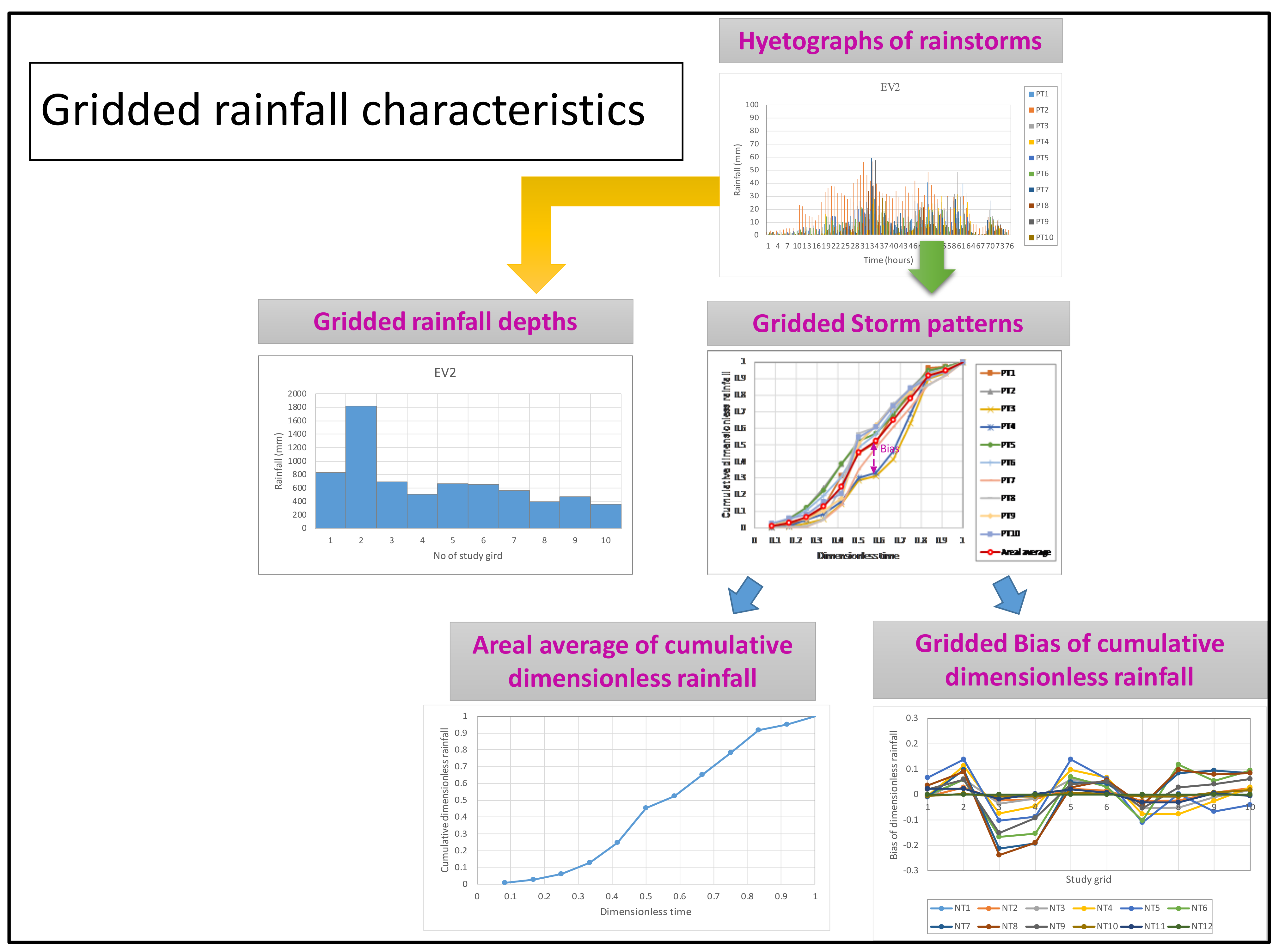
It is well-known that a large training dataset is desired for training the ANN model. Therefore, in this study, the stochastic modeling of gridded short-term rainstorms developed by Wu et al. (2021) (named the SM_GSTR model) is employed to simulate a great number of rainstorms at all grids within the study area. Within the SM_GSTR model, the event-based rainstorm is basically grouped into three rainfall characteristics, including the event-based rainfall duration, gridded rainfall depths, and gridded storm depths composed of the dimensionless rainfalls at the various dimensionless times; with respect to the gridded storm pattern, it can be grouped into two components, the areal average of the dimensionless rainfalls (i.e., the storm pattern) and the associated deviations at the various dimensionless times. Of these, the gridded rainfall characteristics, gridded rainfall depths, and deviations regarding the areal average of the storm patterns are treated as the spatially correlated variates and the areal average storm patterns are regarded as the temporally correlated variates [31]. Figure 1 shows the process of characterizing the gridded rainstorms into five features (i.e., the gridded rainfall characteristics).

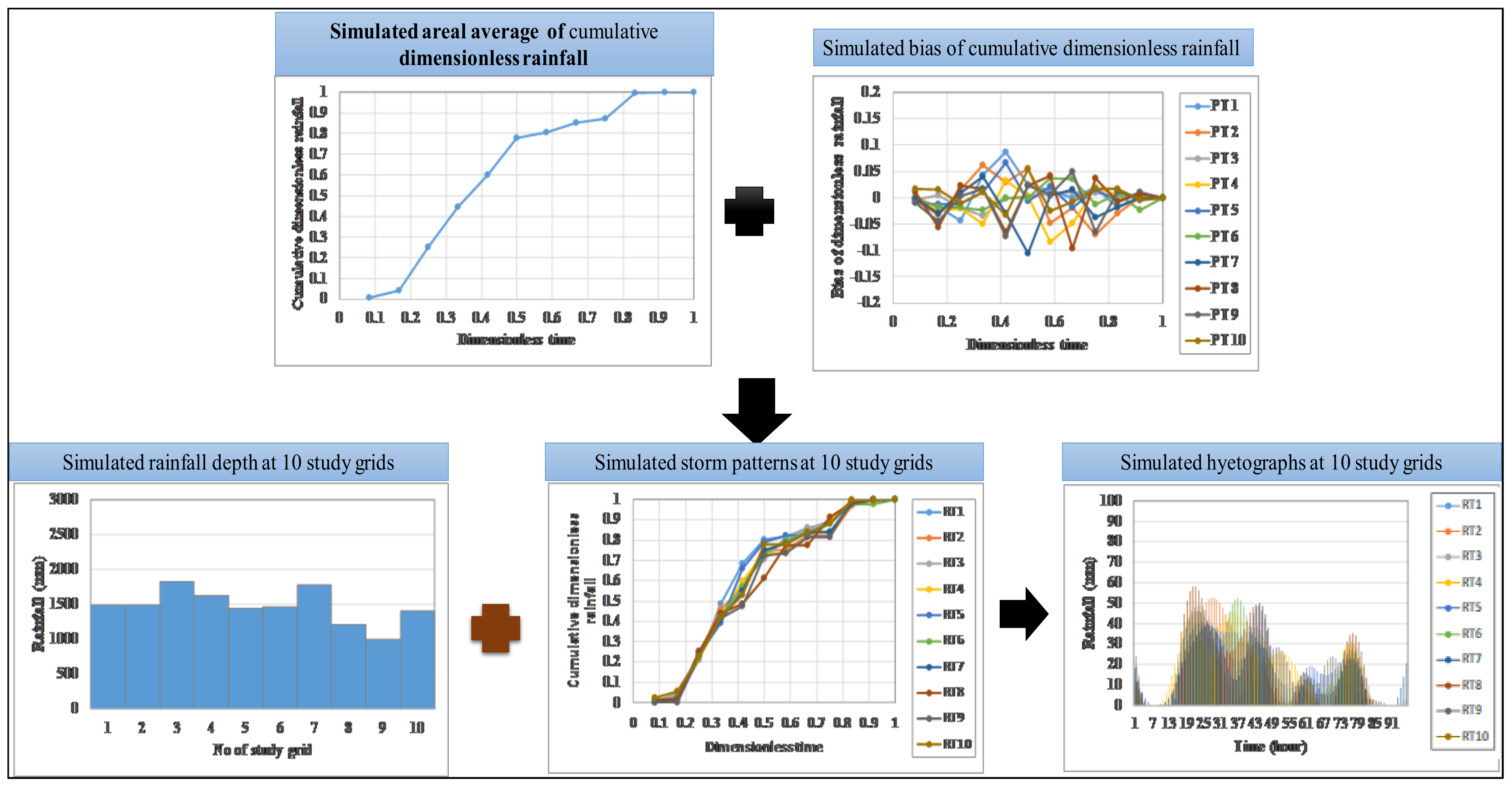
Upon obtaining the gridded rainfall characteristic, within the SM_GSTR model, the non-normal correlated multivariate Monte Carlo simulation approach (Chang et al., 1996) based on the correlation structures of gridded rainfall characteristics in time and space is adopted to generate a desired number of event-based rainfall events through the transform algorithms. The transform algorithms could be employed via the Nataf bivariate distribution model [32], including the transformation to standard normal space, orthogonal transform, and inverse transformation, based on the following correlation relationship:

$${\rho }_{ij}={\int }_{-\infty }^{\infty }{\int }_{-\infty }^{\infty }⌊\frac{x_i-{\mu }_i}{{\sigma }_i}⌋⌊\frac{x_j-{\mu }_j}{{\sigma }_j}⌋{\varnothing }_{ij}(\langle z_i,z_j|{\rho }_{ij}^{\ast }\rangle ){\mathrm{d}z}_i{\mathrm{d}z}_j$$

(1)

$$z_i=\frac{x_i-{\mu }_i}{{\sigma }_i}; z_j=\frac{x_j-{\mu }_j}{{\sigma }_j}$$

(2)

where X_i and X_j are the correlated variables at the points i and j, respectively, with the means ${\mu }_i$ and ${\mu }_j$, the standard deviations ${\sigma }_i$ and ${\sigma }_j$, and correlation coefficient ${\rho }_{ij}$, respectively; i and Z_j are bivariate standard normal variables corresponding to the variables X_i and X_j, with the correlation coefficient ${\rho }_{ij}^{\ast }$ and the joint standard normal density function ∅_ij(∙). To generate a number of variables with high correlation ${\rho }_{ij}$, a set of semi-empirical formulae [33] was derived to modify ${\rho }_{ij}$ in the original space to ${\rho }_{ij}^{\ast }$ in the normal space through a transformation factor T_ij, depending on the marginal distributions and correlation of X_i and X_j, as follows:

$${\rho }_{ij}^{\ast }=T_{ij}\times {\rho }_{ij}$$

(3)

Eventually, the simulated gridded rainstorms can be achieved in accordance with the process of combining the generated gridded rainfall characteristics, as shown Figure 2 [31].

2.3. 2D Inundation Simulation Modeling

Using the estimated runoff hydrograph from the observed and predicted precipitation and tide levels, the water level hydrographs at various cross-sections along the river and at the computation grids within the region can be calculated through the inundation simulation models developed using the depth-averaged Navier–Stokes equation (NSE), named the Saint-Venant shallow water equations. Several numerical models for simulating 2D inundation have been developed based on the NSE, such as SOBEK 1D-2D [32], MIKE 11-21 [34,35], TrimR2D [36], and TELEAC-2D [37] In general, the above inundation-simulation models can be classified into numerical, statistical, and flood inundation mapping models. The hydraulic numerical SOBEK model is a sophisticated one-dimensional open-channel dynamic flow and two-dimensional overland flow modeling system (named SOBEK 1D-2D hydrodynamic model); it can be used to simulate and tackle problems in river management, flood protection, design of canals, irrigation systems, water quality, navigation, and dredging. Therefore, this study uses the SOBEK model to carry out the inundation simulation with a large number of generated grid-based rainstorms.

2.4. Artificial Neural Network Model Associated with Multiply Transfer Functions

It is well-known that the related artificial neural network (ANN) models are frequently adopted in the forecast/estimation regarding flood-rated variates. In spite of the prediction of the hydrological variates being effectively carried out by the ANN-based models, their reliability and accuracy should be influenced by the uncertainties in the transfer function (i.e., activation functions) and selected and associated neuron weights between two layers (i.e., ANN weights) attributed to the variation in the observations [18,38,39]. Moreover, although the back-propagation (BP) algorithm with the gradient descent method is commonly utilized in training the ANN model, the formula of adjusting the connection weights regarding the neurons is difficult to derive under constraint with the transfer functions (or activation function) used. By doing so, the training performance fails to achieve the local optimal values with high likelihood, contributing to the given inappropriate initial values and leaning rate, which leads to the problem with oscillation, thereby reducing the convergence speed [18,22].

Furthermore, the numbers of neurons at hidden layers are significantly increased owing to the performance of training the ANN model. Thus, if few neurons are considered, the corresponding network structure does not easily emulate the underlying function attributed to the insufficient parameters; in contrast, as a result of a great number of the neurons adopted in the network structure, the overfitting problem might occur [40]. Therefore, several methods are proposed to estimate the number of neurons included in

Table 1. Formulae for estimating the number of hidden neurons (Wu et al., 2021) [18].

No of Formulae	Formula	Reference
1	$N_{HN}=\left(\sqrt{1+8\times N_{IP}}-1\right)/2$	Li et al. method [41]
2	$N_{HN}=N_{IP}-1$	Tamura and Tateishi method [28]
3	$N_{HN}=\raisebox{1ex}{$2\times N_{IP}$}\!\left/ \!\raisebox{-1ex}{$N_{IP}$}\right.$+ 1	Zhang et al. method [42]
4	$N_{HN}=\sqrt{N_{IP}\times N_{OP}}$	Shibata and Ikeda method [43])
5	$N_{HN}=2^{N_{IP}}-1$	Hunter et al. method [44]
6	$N_{HN}=\raisebox{1ex}{$\left[4\times {(N_{IP})}^2+3\right]$}\!\left/ \!\raisebox{-1ex}{$\left[{(N_{IP})}^2-8\right]$}\right.$	Sheela and Deepa method [45]

.

Therefore, the network structure and the types of the transfer functions are supposed to be regarded as the uncertainty factors for training the ANN models; to figure out the problem with the above uncertainties in the training of the ANN model, Wu et al. [18] proposed an ANN-derived model (named the ANN_GA-SA_MTF) by adopting the network structure of three layers with multiple transfer functions (see

Table 2. Transform functions commonly used (Wu et al., 2021, Maca et al., 2014) [18,38].

Transfer function		Formula	Derivative
TF1	Logistic (soft step, Sigmoid)	$f\left(x\right)=\frac{1}{1+e^{-\propto x}}$	$f^{\prime }\left(x\right)=f\left(x\right)\left(1-f\left(x\right)\right)$
TF2	Tanh	$f\left(x\right)=\tan h\left(x\right)=\frac{2}{1+e^{-2\propto x}}-1$	$f^{\prime }\left(x\right)=1-f{\left(x\right)}^2$
TF3	Arctan	$f\left(x\right)={\tan }^{-1}\left(\propto x\right)$	$f^{\prime }\left(x\right)=\frac{1}{{\left(\propto x\right)}^2+1}$
TF4	Identity	f(x) = $\propto$x	$f^{\prime }$(x) = $\propto$
TF5	Rectified linear unit (ReLU)	$f\left(x\right)=\left\{\begin{array}{c}0 for x<0\\ 1 for x\ge 0\end{array}\right.$	$f^{\prime }\left(x\right)=\left\{\begin{array}{c}0 for x<0\\ 1 for x\ge 0\end{array}\right.$
TF6	Parametric rectified linear unit (PReLU, leaky ReLU)	$f\left(x\right)=\left\{\begin{array}{c}\propto x for x<0\\ x for x\ge 0\end{array}\right.$	$f^{\prime }\left(x\right)=\left\{\begin{array}{c}\propto for x<0\\ 1 for x\ge 0\end{array}\right.$
TF7	Exponential linear unit (ELU)	$f\left(x\right)=\left\{\begin{array}{c}\propto \left(e^x-1\right)for x<0\\ x for x\ge 0\end{array}\right.$	$f^{\prime }\left(x\right)=\left\{\begin{array}{c}f\left(x\right)+\propto for x<0\\ 1 for x\ge 0\end{array}\right.$
TF8	Inverse abs (IA)	$y\left(x\right)=\frac{x}{1+\left|\propto x\right|}$	$y^{\prime }\left(x\right)=\frac{1}{{\left(1+\left|a\propto x\right|\right)}^2}$
TF9	Rootsig (RS)	$y\left(x\right)=\frac{\propto x}{1+\sqrt{1+{\left(\propto x\right)}^2}}$	$y^{\prime }\left(x\right)=\frac{1}{\left(1+\sqrt{1+{\left(\propto x\right)}^2}\right)\sqrt{1+a{\left(\propto x\right)}^2}}$
TF10	Sech function (SF)	$y\left(x\right)=\frac{2}{\exp \left(\propto x\right)+\exp \left(-\propto x\right)}$	$y^{\prime }\left(x\right)=-y\left(x\right)\tan h\left(\propto x\right)$

) in which the associated ANN weights are calibrated by means of the genetic algorithm based on the sensitivities to model parameters (called the GA-SA algorithm) [29].

To quantify the reliability of the model outputs, the proposed ANN_GA-SA_MTF model is collaborated with a nonparametric method, named the weighted likelihood sample quantile estimator method proposed by Yang and Tung [46], to compute the quantiles of resulting model outputs via the following equation:

$$X_{p,WL}={\sum }_{r\in \omega }{W}_{r,n,WL}{X}_{\left(r\right)}$$

(4)

in which $W_{r,n,WL}=\frac{F_{r,n}\left(p\right)}{{\sum }_{s\in \omega }{F}_{s:n}\left(p\right)}$, with ω being the band width that contains a set of order statistics ($X_{(1)}\le X_{(2)}\le \dots \le X_{(n)}$) that are deemed significant in contributing to the estimation of X_p as a result of the band width being no smaller than 2.0.

In addition to quantifying the reliability of the model estimates using the results from the ANN_GA-SA_MTF model, the weighted averages of model estimates are issued as forecasts using the following equation:

$${\widehat{Y}}_{WA}={\sum }_{i=1}^{N_{TF}} \left[W_{TF}^i\times \widehat{Y}\left({\theta }_{T{F}_i}^j\right)\right]$$

(5)

$$W_{TF}^i=\frac{\frac{1}{E\left({\theta }_{TF}^i\right)}}{{\sum }_{i=1}^{N_{TF}}\frac{1}{E\left({\theta }_{TF}^i\right)}}$$

(6)

in which $N_{TF}$ is the number of transfer functions considered; $Y_k \mathrm{and} {\widehat{Y}}_k\left({\theta }_{TF}^i\right)$ denote the observed hydrological data and estimated ones by the ANN_GA-SA_MTF model with the jth set of the appropriate parameters ${\theta }_{TF}^i$, respectively; and $W_{TF}^i$ represents the weighted factor of the ith transfer function with the appropriate parameters ${\theta }_{TF}^i$ calculated, with the $E\left({\theta }_{TF}^i\right)$ being the objective-function value (i.e., the root mean square error, RMSE).

In particular, to provide more reliable and accurate model outputs, the real-time error correction method established using the time-series approaches and Kalman filtering [30] is adopted within the ANN_GA-SA_MTF to immediately adjust the forecasts ($Y_{corr}^{t_{pred}}$) based on real-time observations through the Internet of Things (IoT) using the ANN_GA-SA_MTF model by means of the following equation:

$$Y_{corr}^{t_{pred}}=Y_{pred}^{t_{pred}}+{\epsilon }_{TS}^{t_{pred}}+{\epsilon }_{KF}^{t_{pred}}$$

(7)

where $Y_{pred}^{t_{pred}}$ stands for the model estimates (i.e., the forecasts); and ${\epsilon }_{TS}^{t_{pred}} \mathrm{and} {\epsilon }_{KF}^{t_{pred}}$ serve as the forecast error estimated by the time series approaches and Kalman filtering method, respectively.

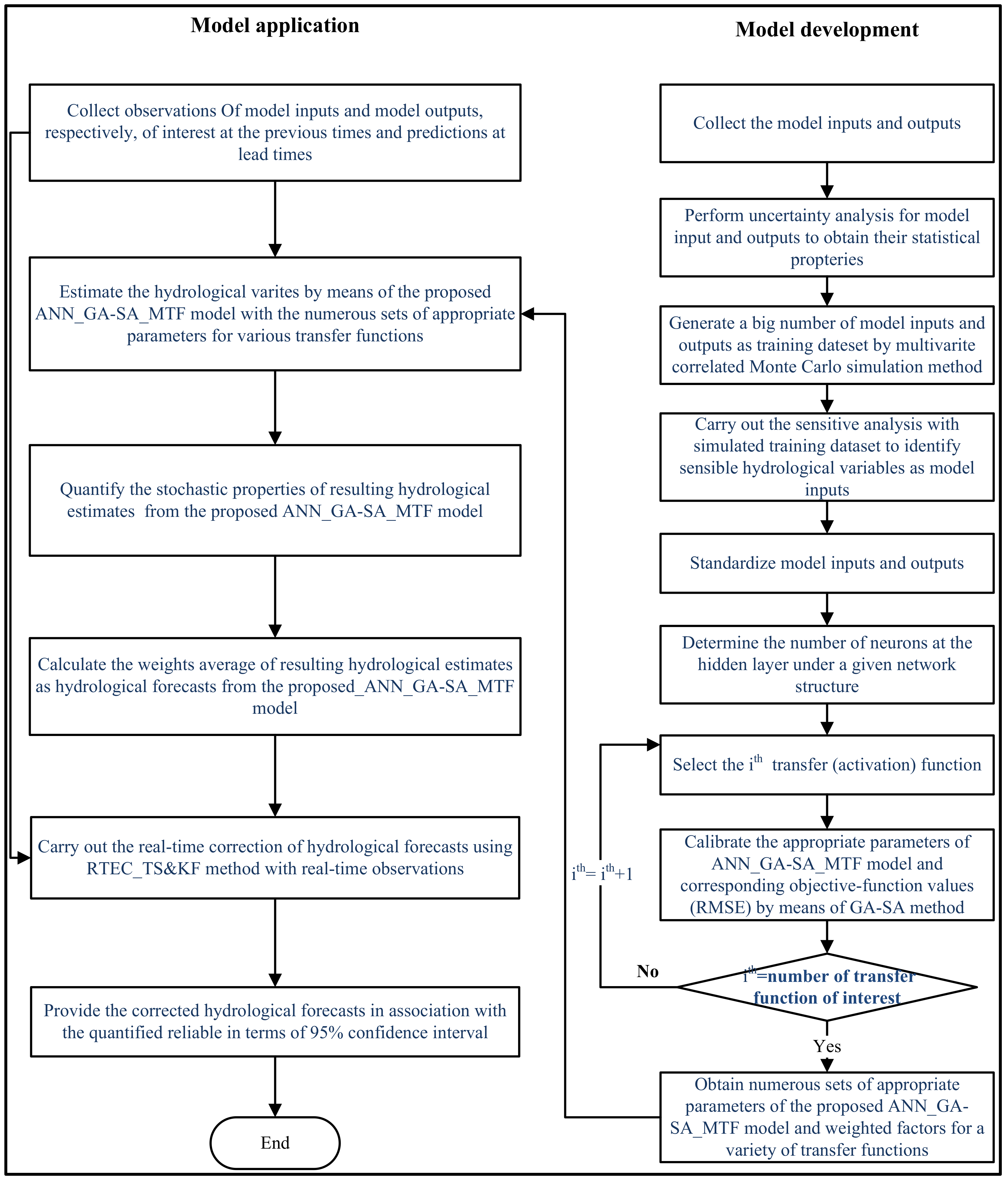
In summary, the framework of developing the ANN_GA-SA_MTF model is generally classified into the four steps (see Figure 3): the parameter calibration using the GA-SA approach, the reliability quantification of model outputs, the estimation of model outputs, and the real-time correction of model outputs; the associated concepts are briefly introduced as follows.

2.5. Model Formulation

To sum up the aforementioned concepts, this study intends to utilize the ANN_GA-SA_MTF model to develop a smart model for forecasting the inundation depth at the roadside IoT sensors, named the SM_EID_IOT model. As a result of the inundation being significantly increased by the rainstorm, the inundation depths at the specific locations, where the IoT sensors are set up, should be temporally and spatially related to the rainfalls and inundation depths at the previous time steps during an event (Notaro et al., 2013; Lyu et al., 2018). Although the resolution of the rainstorm in space obviously impacts the estimation of the flood/inundation, the areal average rainfalls calculated from a number of the raingauges within the small basin are frequently applied in the hydrological/hydraulic analysis under simplification of the rainfall-runoff simulation [47]. Therefore, in this study, in addition to the uncertainties in the resolutions of the rainfall and inundations in time (i.e., the forward time step from the current time), the distances to the IoT sensor for calculating the areal-average rainfall with the rainfalls at the grids (i.e., gridded rainfall) is treated as the uncertainty factor calculated through the following equation:

$${\overline{R}}_{IOT}^t=\frac{1}{N_g}{\sum }_{i=1}^{N_g}{R}_i^t$$

(8)

where ${\overline{R}}_{IOT}^t$ accounts for the areal-average rainfall at the IoT sensor; $N_g$ is the number of the grids, the distance of which to the IoT senor is equal to or less than the specific critical distance (i.e., critical spatial resolution); and L_c and $R_i^t$ serve as the gridded rainfalls for the time step t-hour at the ith grid.

Therefore, on the basis of the ANN_GA-SA_MTF model with generated rainfall-inundation depths and associated gridded rainstorms, this study establishes the relationship of the inundation depths at the IoT sensors with the inundation depths and rainfall at the lead times, as well as the previous time steps, and the inundation depths at the forward time step can be written as follows:

$${\widehat{h}}_{IOT}^{t+1}=f_{{\mathrm{ANN}}_{\mathrm{GA}}-\mathrm{SA}\_\mathrm{MTF}}\left({\overline{R}}_{IOT}^{t+1},{\overline{R}}_{IOT}^t\cdots {\overline{R}}_{IOT}^{t-T_c-1},h_{IOT}^t,\cdots h_{IOT}^{t-T_c-1}\right)$$

(9)

in which T_c serves as the critical values of the resolutions in time (i.e., critical temporal resolution); ${\widehat{h}}_{IOT}^{t+1}$ is the inundation-depth estimate for the lead time (t + 1 h); ${\overline{R}}_{IOT}^{t+1}$ denotes the rainfall forecast at the lead time (t + 1 h); ${\overline{R}}_{IOT}^t,\cdots {\overline{R}}_{IOT}^{t-T_c-1}$ account for the areal average rainfall at the current time (t hour) and those from the forward T_R hours calculated from the gridded rainfalls within the specific critical spatial resolution, i.e., the distance L_c to the IoT sensor; and $h_{IOT}^t,\cdots h_{IOT}^{t-T_c-1}$ represent the observed inundation depths from the t hour to the t-T_h hours under consideration of the critical temporal resolution (i.e., the forward time steps T_h.). Note that the critical values of the resolution in time and space T_R and T_h can be determined by evaluating the spatially and temporally varying trend of the at-site inundation depth with the areal average rainfall via the correlation and sensitivity analysis in this study.

2.6. Model Framework

According to the aforementioned concepts, the development and application of the proposed SM_FIDEP_IOT model can be grouped into six parts: (1) generation of the rainstorm events at all grids within the study area; (2) 2D rainfall-induced inundation simulation; (3) extraction of the at-site inundation depths and corresponding rainfall at neighboring grids; (4) identification of critical resolution in time and space; (5) development of the proposed SM_EID_IOT model on the basis of the ANN_GA-SA_MTF model; and (6) integration with the real-time error correction (RTEC_TS&KF) method to adjust the inundation-depth estimates. The detained framework of the model development and application are addressed as follows.

2.6.1. Model Development

Step 1

Collect the historical rainstorm events at all grids within the study area and extract their gridded characteristics, i.e., rainfall duration, gridded rainfall depth, areal average of cumulative dimensionless rainfall, and the associated bias.

Step 2

Reproduce a great number of rainfall fields with high spatiotemporal resolutions comprised of the simulated gridded rainfall characteristics by the SM_GSTR model with the results from uncertainty analysis using the observations obtained in Step [1].

Step 3

Carry out the 2D inundation simulation by means of the SOBEK model with a great number of gridded rainstorms simulated in Step [2] to obtain the simulations of inundations depths at the IoT sensors.

Step 4

Extract the simulated inundation depths at the IoT sensor under consideration of different periods (i.e., critical temporal resolution) and the corresponding simulated rainfalls at the neighboring girds within the specific distances to the IoT sensor (i.e., critical spatial resolution).

Step 5

Perform correlation and sensitivity analysis to determine the appropriate critical resolutions in time and space.

Step 6

Calculate the areal average rainfalls from the simulations of the gridded rainfall under the consideration of critical temporal and spatial resolutions determined in Step [5].

Step 7

Calibrate the parameters of the ANN_GA-SA_MTF model used in the estimation of inundation depths via the proposed SM_EDI_IOT model using the simulations of the inundation depths at the IoT sensor and corresponding areal average rainfalls.

2.6.2. Model Application

Step 1

Collect the observed inundation depths during the rainfall-induced flood event at the IoT sensor and calculate the corresponding areal average rainfalls under the conditions of the appropriate temporal and spatial resolutions.

Step 2

Obtain the resulting inundation-depth estimate at the lead times and associated 95% confidence intervals from the proposed SM_EID_IOI model.

Step 3

Carry out the real-time correction regarding the resulting inundation-depth estimates at the lead times from the proposed SM_EID_IOT model with the RTEC_TS&KF method in accordance with the bias of the inundation-depth estimates in comparison with the observations at the forward time steps during the event.

3. Study Area and Data

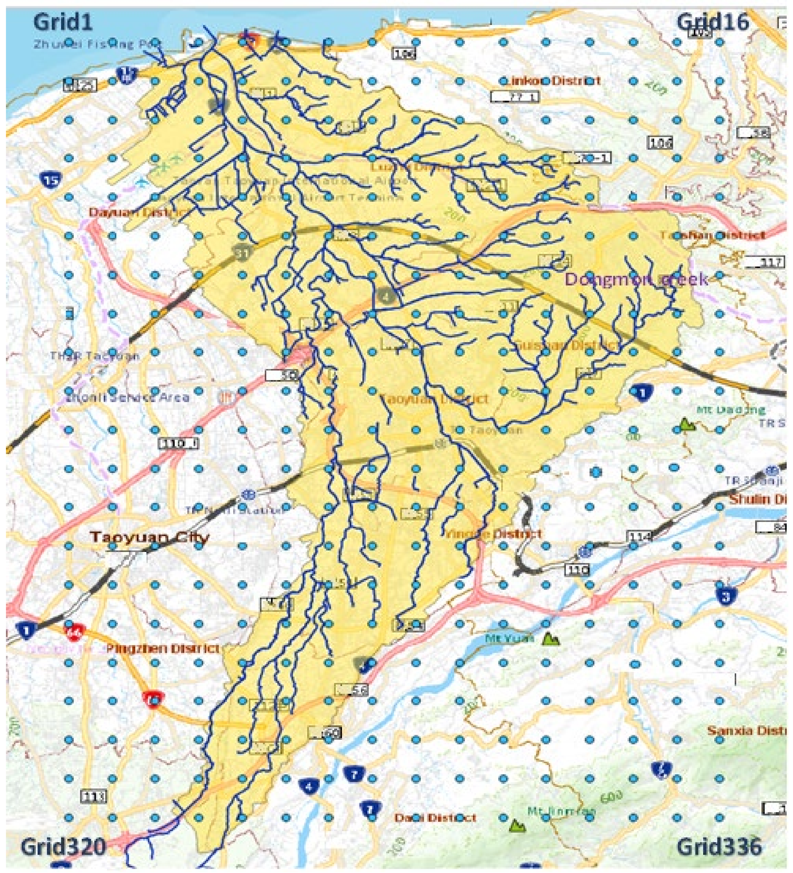
The Nankan River—whose length and drainage area and slope are 31 km and 224 km², respectively (see Figure 4)—in Taoyuan County is one of the most polluted rivers in northern Taiwan; further, its average slope and mountain area are about 0.0077 and over 900 m, respectively. Additionally, it flows through Guishan, Taoyuan, and Luzhou Districts in Taoyuan City, including six riverside parks and three branches, Dongmon Creek, KengZi Creek, and Kengzi Creek. Of the aforementioned branches, Dongmon Creek is frequently inundated as a result of a reduction in the number of detention ponds and the cross-section area in the river channel. Note that, within the Nankan River watershed, Taiwan Central Weather Bureau (CWB) provides the quantitative precipitation estimation (QPE) with a spatial resolution of 1.5 km × 1.5 km, i.e., the rainfall data of 336 grids (called QPE grids), as shown in Figure 4.

As the purpose of this study is to develop a stochastic ANN-derived model using the training datasets comprising a great number of the rainfall-induced 2D inundation simulations with high resolution in time and space, the hourly rainfall of 20 rainstorm events at 336 grids within the study area (Nankan River watershed) (see

Table 3. Summary for hydraulic facilities, hydrological analysis, and topographic features used in the SOBEK model for the Nankan River watershed.

Hydraulic Facility	Number	Hydrologic Analysis	Model
1. Sub-basins	579	Rainfall-runoff modeling	SCS UH
2. Cross-sections	3219	Topographic feature	Measurement date
3. Gates	18	1. Digital elevation map	2012
4. Bridges	90	2. Map for land-use	2014
5. Sewer	1386	Hydraulic factors Kn	Magnitude
6. Manholes for sewer system	1382	Roughness coefficient	0.2–0.45

) is adopted as the study data.

Figure 5 shows the hyetographs of the 20 selected radar-based rainstorm events (2005–2017) provided by Taiwan Central Weather Bureau. According to the process of extracting the gridded rainfall characteristics, the gridded rainfall depths and storm patterns of the concerned 20 rainstorm events in the study area can be obtained. Therefore, upon establishing the proposed SM_EID_IOT model, the uncertainties in the gridded rainfall characteristics should be taken into account and quantified for the simulations of the rainstorm events at all grids within the study area. Accordingly, big data regarding the 2D rainfall-induced flood events can be generated at the training and validation datasets.

4. Results and Discussion

4.1. Simulation of Rainfall-Induced Inundation

Before carrying out the rainfall-induced inundation, a great number of the gridded rainstorms should be reproduced in advance. Thus, in this study, using the SG_GSTR method with the above statistical moments of gridded rainfall characteristics, 1000 simulations can be obtained. After that, the SOBEK 1D-2D hydrodynamic model is employed to carry out the inundation simulation with 20 m × 20 m DEM of Nankan River watershed provided by Water Resource Agency in Taiwan (see Figure 5). Figure 6 presents the river-channel internet and computation nodes in the SOBEK 1D-2D dynamic model set up according to the geographical and hydrological data in the study area. Within the Nankan River watershed, a mesh composed of 335 × 520 computation grids whose the spatial resolution is 20 m × 20 m is adopted. The above topographic, hydrologic, and hydraulic features used in Nankan River SOBEK model are listed in Table 3. Finally, using the SOBEK model for the Nankan River watershed with 1000 simulations of the gridded rainstorm events, the resulting 2D inundation simulations, including the gridded inundation depths and corresponding flooding area, could be accordingly obtained.

Thereby, this study implements the 2D inundation simulation by taking into account the spatiotemporal uncertainty in the rain field to achieve the goal of providing detailed 2D inundation information with high spatial and temporal resolution as the training datasets for the proposed SM_EID_IOT model.

4.2. Identification of Potential Locations of Roadside IoT Sensors

On the basis of the results from the simulated grid-based inundation depths within the study area, a 2D inundation simulation with high spatial and temporal resolution can be used to determine the locations of the roadside water-level sensors. In detail, the road-side water-level sensors can be set up at the locations in association with high flooding frequency calculated from the above 2D inundation simulations for the correction of flooding forecasts [30]. Under the consideration of IoT quality, the most appropriate locations of roadside water-level sensors can be accordingly determined and named IoT sensors.

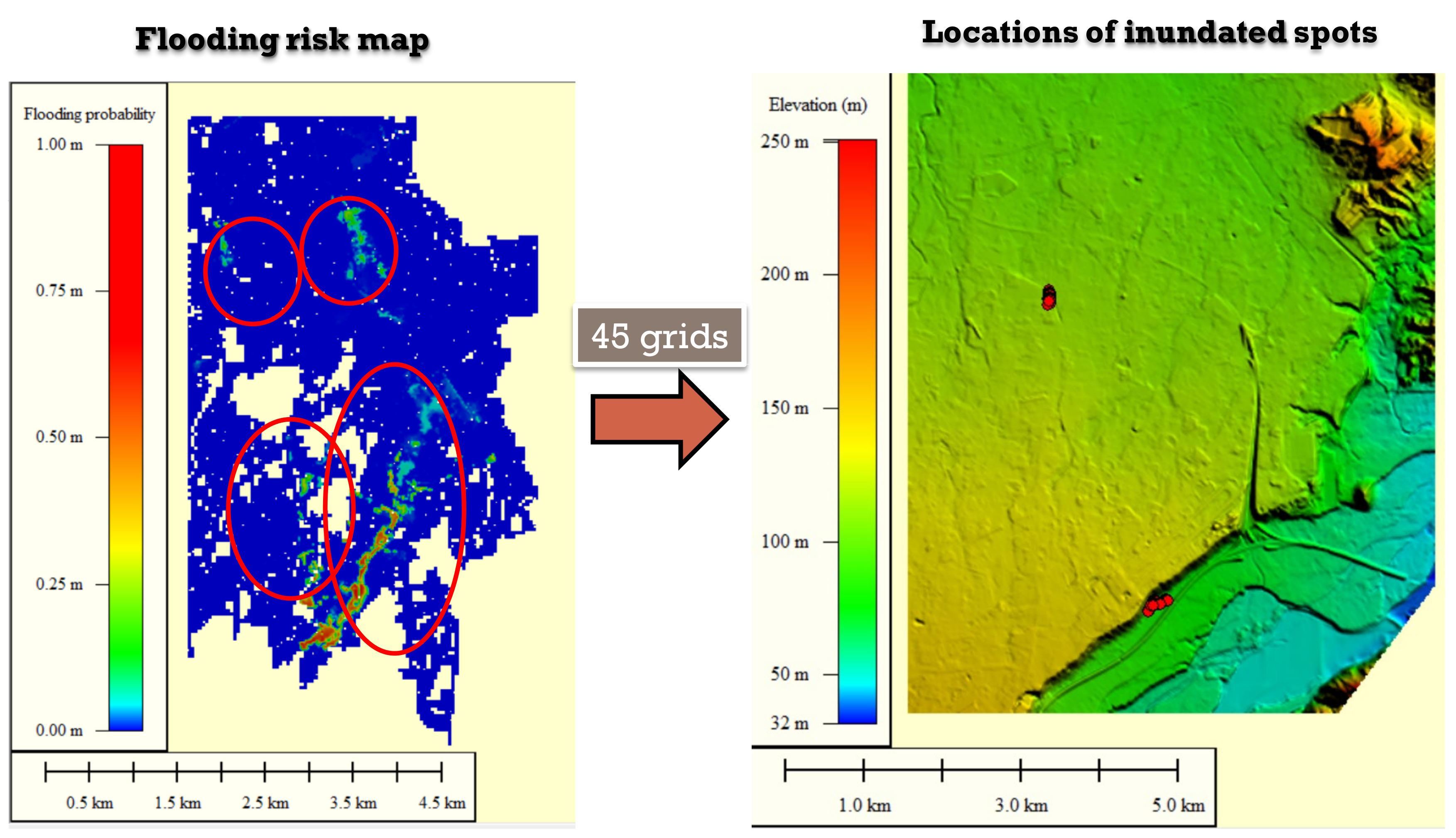
To quantify the flooding risk at all grids, this study utilizes the following equation to calculate the flooding probability ($P_f\left(h_f>0\right)$) within the study area, the Nankan River watershed (see Figure 4):

$$\begin{array}{c}{P}_f\left(h_f>0\right)=\frac{{{\displaystyle \sum }}_{i=1}^{N_{GRS}}\left(I_f\left(h_f^i\right)\right)}{N_{GRS}}\\ I_f\left(h_f^i\right)=1, if max\left(h_f\right)>0_{}^{}\\ I_f\left(h_f^i\right)=0, if max\left(h_f\right)=0_{}^{}\end{array}$$

(10)

where $I_f\left(h_f^i\right)$ is the flooding indicator and $max\left(h_f\right)$ stands for the maximum gridded inundation. In Equation (10), if the maximum of gridded inundation depth is greater than zero, the corresponding flooding probability $I_f\left(h_f^i\right)$ is equal to one; otherwise, it is equal to 0. Thus, in reference to Figure 7, it can be seen that inundation mainly takes place in the four regions. Apparently, the first 46 grids associated with high flooding probabilities (approximately 0.7) can be identified in the two locations marked with a red line, near the locations (TWD97X:280200.2, TWD97Y:2765356.7) and (TWD97X:281523.6, TWD97Y:2761435.5), respectively; they can be treated as the potential inundated grids. Therefore, among the aforementioned potential inundated spots, the locations of desired roadside IoT sensors can be determined.

In conclusion, the quantification of flood risk at all grids within the study area can be carried out using a large number of inundation simulations by the hydraulic numerical model with the generated grid-based rainstorm events through the proposed SM_GSTR model. Additionally, the resulting big data of rainfall-inundation simulations are advantageous to the identification of roadside inundation-depth sensors, which can be used in the real-time error correction of flood forecasts [1].

As the Nankan River watershed lacks practical roadside IoT sensors, the grid with high flooding risk, the TWD97 coordination of which is (TWD97X: 281523.6, TWD97Y: 2761435.5), is selected as the potential IoT sensor. As a result, the corresponding simulations of rainfall-induced inundation, consisting of the inundation depths and associated areal average rainfalls, are employed in the development and validation of the proposed SM_EID_IOT model.

4.3. Determination of Critical Resolutions in Time and Space

In this study, the correlation and sensitivity analysis for the inundation depth at the IoT sensor of interest (TWD97X: 281523.6, TWD97Y: 2761435.5) is carried out to detect the appropriate critical value of the spatial and temporal resolutions. In detail, the critical distance to the IoT sensor for calculating the areal average rainfalls and the forward time steps from the current time for selecting the observed inundation depths and areal average rainfalls are required for deriving Equation (9) within the proposed SM_EID_IOT model.

4.3.1. Critical Resolution in Space

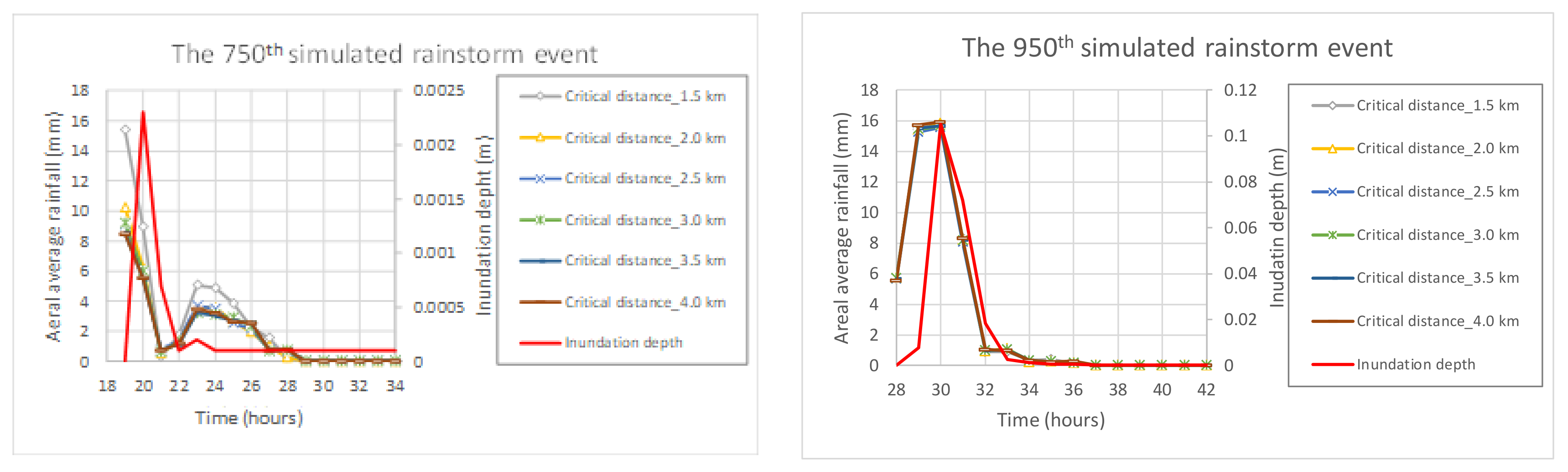
To quantify the fitness of the areal average rainfall for various critical distances to the inundation depth, Pearson correlation coefficients (ρ) are adopted, as shown in Figure 8, presenting that most correlation coefficients gradually increase/decrease with the critical distances, i.e., the critical spatial resolution L_c used in Equation (9). For example, regarding the 5th, 500th, and 1000th simulation cases, the correction coefficient generally declines from the critical distance of 1.5 km to 4 km critical distance; it then remains constant. Contrarily, in the case of the remaining simulation cases, the correlation coefficient remains constant.

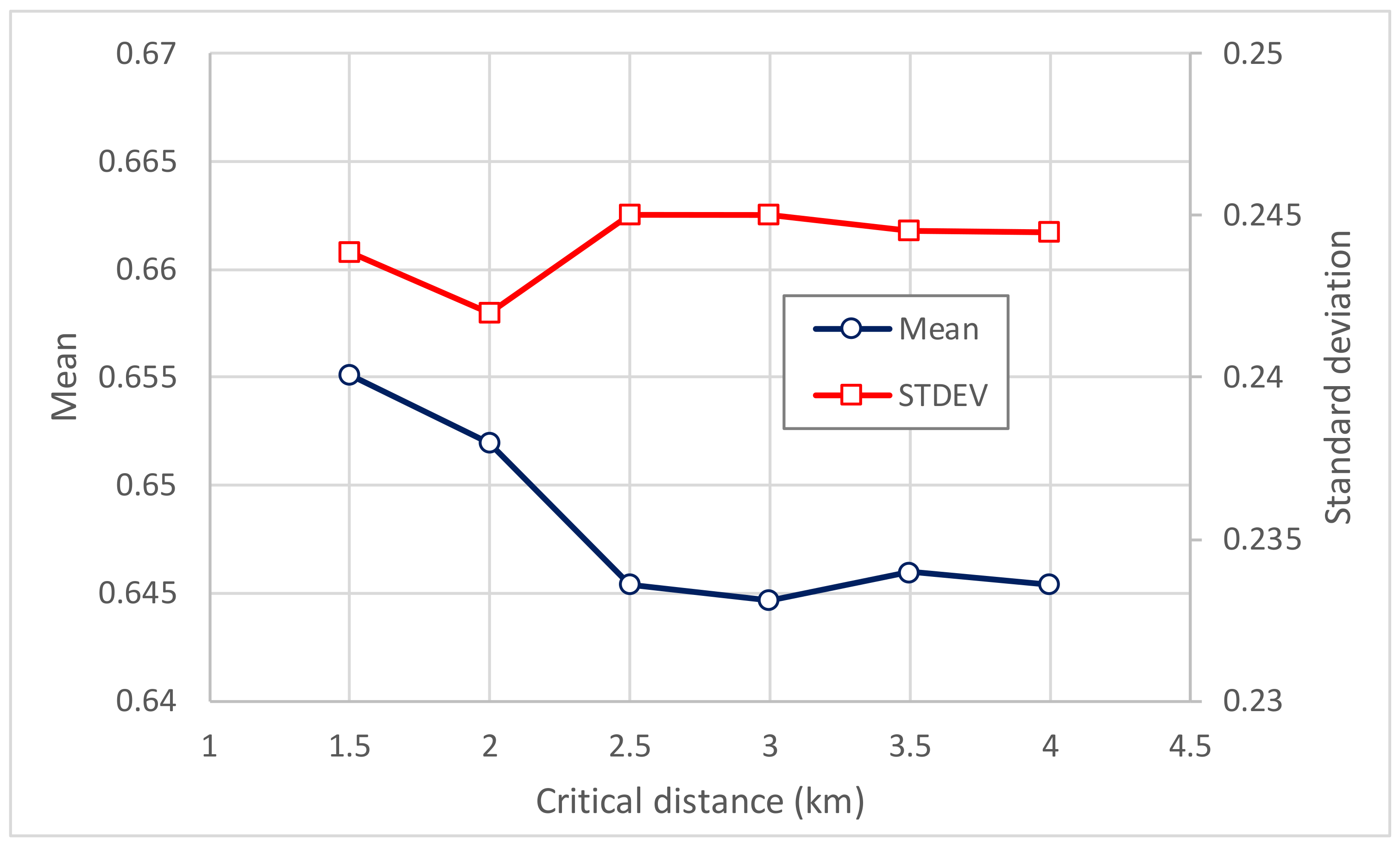
To quantify and assess the effect of critical distances regarding the calculation of areal average rainfall on the estimated inundation depth, the statistical properties of Pearson coefficients (i.e., mean value μ and standard deviation σ) calculated from 1000 simulation cases are computed as shown in Figure 9, where the mean value of the correlation coefficient ρ declines with the critical distance from 1.5 km (ρ = 0.655) km to 3 km (ρ = 0.645), and the correlation coefficient then reaches its constant value (ρ = 0.645); further, its standard deviations for various critical distances approximate 0.69, except for the 2 km critical distance (σ = 0.688).

To sum up, the above results from the correlation analysis reveals that, in spite of the 2 km distance having the smallest variation, the areal average rainfall calculated from the precipitations at the grids, the distance of which to the IoT sensor is less than or equal to 3 km, exhibits a stable variation in terms of the correlation coefficient. In conclusion, the critical resolution in space is assigned as 3 km for the calculation of the areal average rainfalls.

4.3.2. Critical Resolution in Time

Generally speaking, the water level at the current time is markedly related to the areal average rainfall and inundation depths at the previous time steps. Thus, the temporal resolution of the areal average rainfall and inundation depths in terms of the correlations within the specific forward time steps, i.e., critical temporal resolution T_c hour in the standardized regression equation, possibly affect the estimation of the inundation depths at the current time step for the IoT sensors. The standardized regression equation is as follows (Speed and Yu, 1993):

$$\frac{Y-\overline{Y}}{S_Y}={\sum }_{i=1}^n{\beta }_i\frac{X_i-{\widehat{X}}_i}{S_{X_i}}$$

(11)

where Y and X are the model output and inputs; $\overline{Y}$ and $\widehat{X}$ account for the mean of the model output and inputs, respectively; $S_Y$ and $S_X$ separately represent the corresponding standard deviation; and ${\beta }_i$ denotes the regression coefficient that is inversely related to the model outputs; otherwise, the model parameter is proportional to the model output in the case of the associated ${\beta }_i$ being positive. Note that the standard regression coefficient ${\beta }_i$ accounts for the sensitivities of the ith model parameter to the model outputs, meaning that a larger absolute value indicates that the change in the ith model parameter more significantly impacts the estimation of the model outputs. Moreover, the model parameter is associated with the negative ${\beta }_i$. Accordingly, the above specific forward period k hours should be treated as the sensible factors, which can be determined based on the regression coefficients β (i.e., the sensitivity coefficient) of the standard regression Equation (11).

In this study, using 1000 simulations of the rainfall-induced inundation, the inundation depths at the six particular time steps—0.3, 0.5, 0.6, 0.7,0.8, and 0.9 times the duration—and the inundation depths as well as the areal average rainfall at the forward 6 h are used in the establishment of the standard regression equation; their resulting regression coefficients could be obtained as shown in Figure 10. By observing Figure 10, the average of absolute sensitivity coefficients regarding the areal average rainfall and inundation depths at the forward 1–6 h, it is known that, with respect to the inundation depth, the average of the absolute sensitivity coefficients of the forward period from T_c = 1 h to T_c = 3 h ranges between 0.563 and 0.43, which are obviously greater than the coefficients regarding the forward T_c = 4 h to T_c = 6 h (about 0.029–0.127). Furthermore, in the case of the areal average rainfall, the absolute sensitivity coefficients corresponding to the forward 3 h change on average from 0.123 to 0.426, which are significantly greater than the coefficients at the forward 4–6 h (approximately 0.015–0.048).

To sum up the above results, the inundation depths at a particular time step are strongly and significantly related to the areal average of rainfall and inundation depths at the forward T_c = 3 h. Therefore, in referring to Equation (9), the relationship of the estimated/forecasted inundation depth regarding the lead time (t + 1 h) at a specific IoT sensor ${\widehat{h}}_{IOT}^{t+1}$ with the observation of the areal average rainfall at the lead time (t + 1 h) and current time (t hour) as well as the forward 2 h and the inundation depths at the forward 3 h (i.e., t, t − 1 and t − 2 h) can be written as follows:

$${\widehat{h}}_{IOT}^{t+1}=f_{ANN-GA-MTF}\left({\overline{R}}_{IOT}^{t+1},{\overline{R}}_{IOT}^t,{\overline{R}}_{IOT}^{t-1},{\overline{R}}_{IOT}^{t-2},h_{IOT}^t,h_{IOT}^{t-1},h_{IOT}^{t-2}\right)$$

(12)

where ${\overline{R}}_{IOT}^t$ is the rainfall forecast at the lead time (t + 1 h); ${\overline{R}}_{IOT}^t,{\overline{R}}_{IOT}^{t-1}, \mathrm{and} {\overline{R}}_{IOT}^{t-2}$ are the areal average rainfalls calculated using the gridded rainfall at the current time (t hour) and forward 2 h (t − 1 and t − 2 h) within the distance of 3 km to the location of the IoT sensor; and $h_{IOT}^t,h_{IOT}^{t-1}, \mathrm{and} h_{IOT}^{t-2}$ represent the observed inundation depths at the current time (t hour) and forward 2 h (t − 1 and t − 2 h).

4.4. Development of the Proposed SM_EID_IOT Model

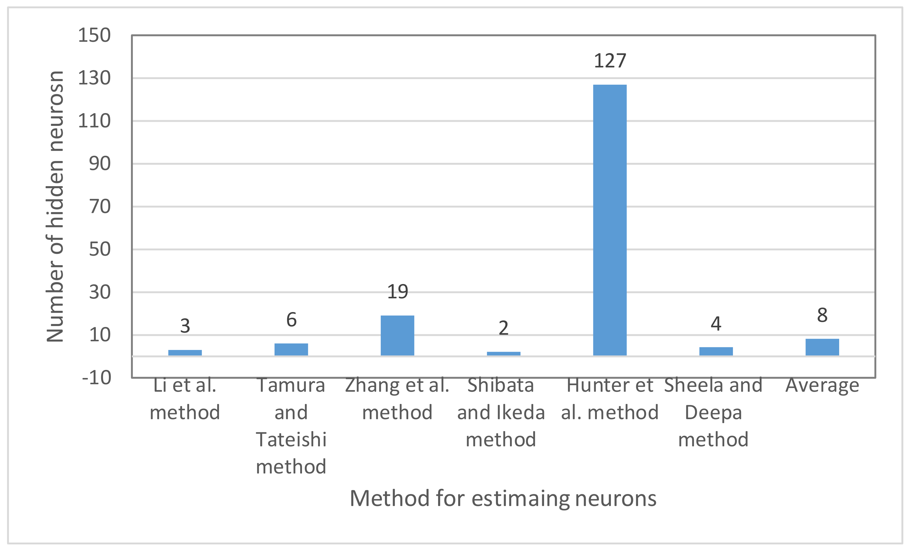
In referring to the framework of the model development, the proposed SM_EID_IOT model for estimating the inundation depths at the lead time regarding the IoT sensor is developed based on the ANN-derived ANN_GA-SA_MTF model by taking into account the uncertainty factors, including the areal average rainfall at the lead time and forward 3 h and the inundation depths at the forward 3 h. Furthermore, according to the induction to the ANN_GA-SA_MTF model, the initial conditions regarding the parameters should be given in advance, including the number of the hidden layers, the total number of neurons used, and the candidate transfer functions, as listed in Table 2. It is well-known that the three-layer network structure, comprising one input layer, one output layer, and one hidden layer, is commonly adopted in hydrological/hydraulic modeling (e.g., Wu et al., 2021); thus, the hidden layer used in the derivation of the SM_EID_IOT model is derived on the basis of the three-layer ANN-based model (i.e., the ANN_GA-SA_MTF model). Moreover, in general, the number of neurons in the entire ANN network structure can be set up by means of a variety of formulae listed in Table 1 in accordance with the number of model inputs and outputs. Figure 11 indicates the resulting number of neurons from the different equations, ranging from 3 neurons to 127 neurons. Accordingly, their average number of 8 neurons is employed in the model development. In addition, the statistical properties, the mean and standard deviation, of the ANN weights are assigned as 0 and 1, respectively. As for the remaining parameters, their initial conditions can be referred to in

Table 4. Definition of parameters used in the proposed ANN-GA-SA_MTF model.

Parameters	Definition
Transfer functions used	TF1-TF10
Input factors	Average rainfall	${\overline{R}}_{IOT}^{t+1},{\overline{R}}_{IOT}^t,{\overline{R}}_{IOT}^{t-1},{\overline{R}}_{IOT}^{t-2}$
	Inundation depth	$h_{IOT}^t,h_{IOT}^{t-1},h_{IOT}^{t-2}$
Output factor	Inundation depth	${\widehat{h}}_{IOT}^{t+1}$
Number of hidden levels	1
Number of neurons	8
Calibration of parameters of transfer function	Number of optimizations	10
	Weights of neurons (${\omega }_{HL})$	Mean	1
		Standard deviation	3
	Bias of function (${\theta }_{TF})$	Mean	0
		Standard deviation	1
	Adjusting factor (${\propto }_{TF})$	Mean	1
		Standard deviation	0.005

.

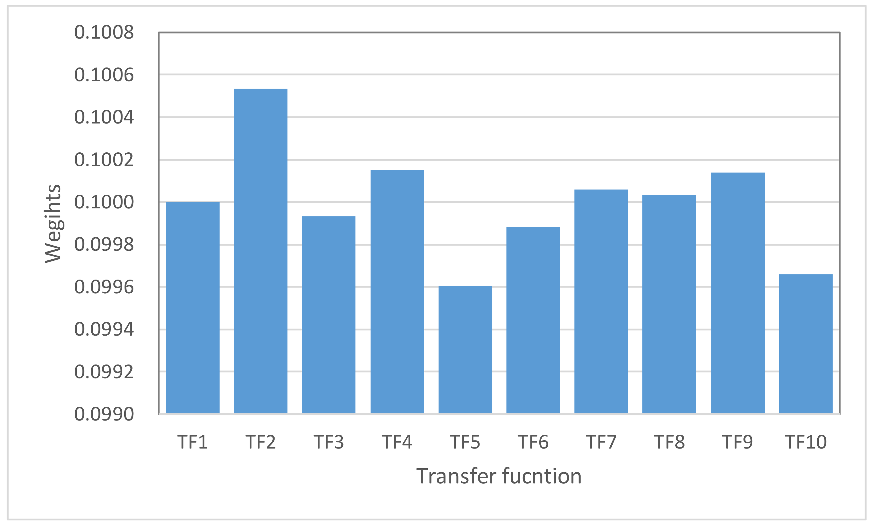
Using the parameter definition shown in

Table 5. Summary for the calibrated parameter of the SM_EID_IOT model in the study area (the Nankan River Watershed).

Transfer Function	$\mathbf{Adjust} \mathbf{Factor} \left({\propto }_{\mathit{T}\mathit{F}}\right)$	0.99139
TF1 (Sigmoid)	Connection weights of neurons ${\omega }_{HL}$	First Hidden Layer		Model Inputs at Input Layer
				1		2	3	4	5	6	7	Bias
		Neuron	1	2.105		−0.146	−3.114	−3.035	1.756	−3.039	−3.355	0.169
			2	1.879		−0.267	2.018	−3.344	−1.904	−0.069	−4.633	−2.275
			2	1.898		3.023	−3.828	−2.855	4.008	−1.024	4.944	−3.015
			4	−0.186		−1.392	2.213	1.737	4.005	6.746	−2.054	−0.052
			5	−1.372		2.638	−1.166	−3.536	1.961	−2.736	−3.007	−0.043
			6	3.729		−3.363	−2.254	−0.530	−4.844	4.774	2.666	5.212
			7	5.364		0.546	5.105	0.169	−4.981	2.625	2.180	3.198
			8	10.950		−3.238	6.896	−1.404	−5.472	1.547	−4.310	−4.908
		Output layer		Connection neurons at the first hidden layer
		Model output	1	1	2	3	4	5	6	7	8	Bias
				−0.264	−0.002	0.357	0.136	−0.560	−1.682	−0.582	0.368	0.085

, the SM_EID_IOT model can be developed by training the ANN_GA-SA_MTF model with 650 simulations of the training datasets, extracted from 1000 rainfall-induced inundation simulations obtained in Section 4.1 and Section 4.2. Table 5 summarizes the results from the parameter calibrations under consideration of the transfer function TF1 (Sigmoid function). Furthermore, according to Figure 12, the inundation-depth estimates are the weighted average using the model estimates resulting from a variety of transfer functions with the corresponding weights, as shown in Figure 13, in which TF2 (Tanh function) and TF5 (ReLU function) are associated with the maximum and minimum weights, 0.10045 and 0.0996, respectively, indicating that the various transfer functions significantly contribute to different degrees to the estimation of the inundation depths at the IoT sensors. Consequently, it is necessary to take into account the effect of uncertainty in the formulation of the transfer functions on the estimation of model outputs via the proposed SM_EID_IOT model.

4.5. Model Validation

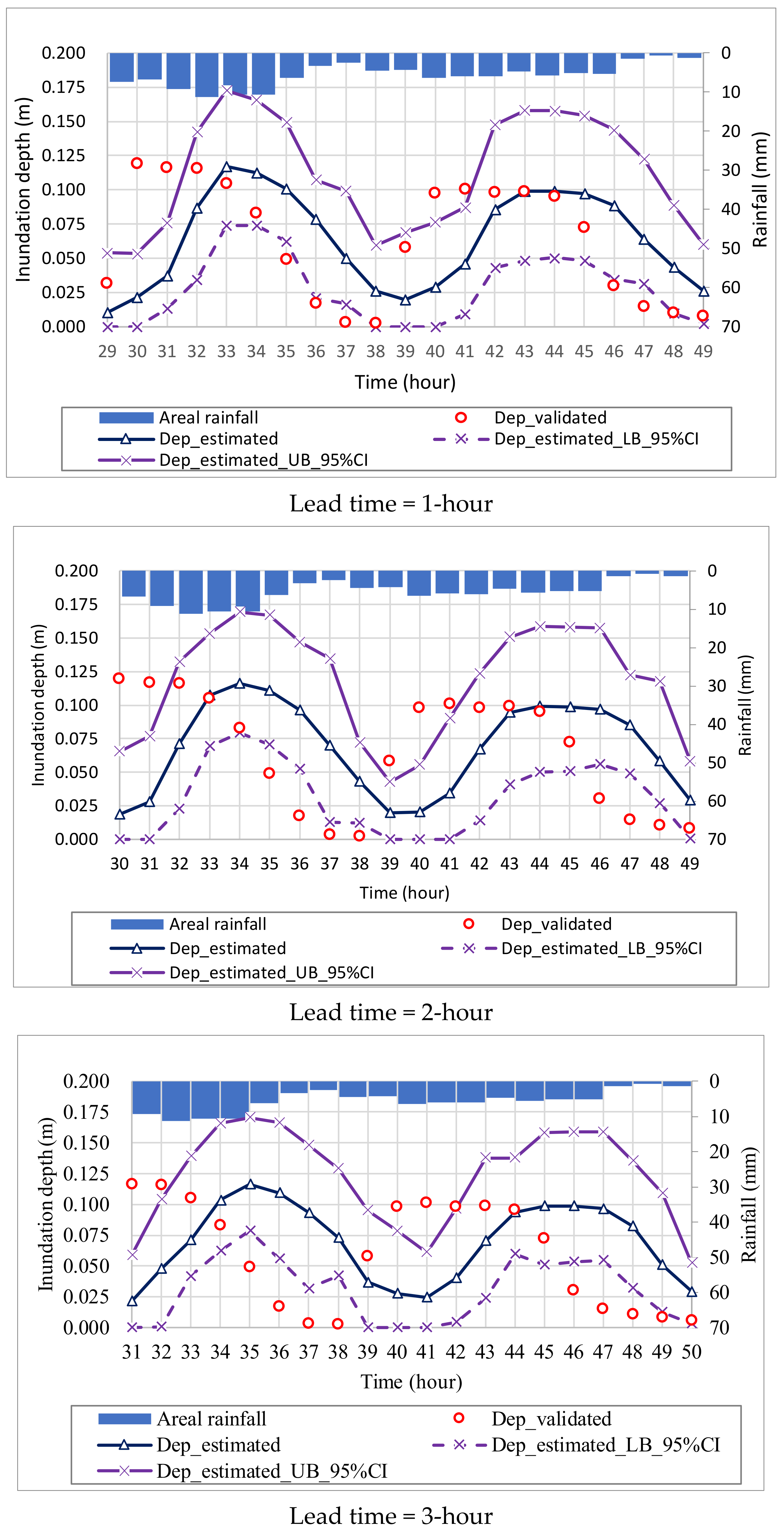
To demonstrate the reliability and accuracy of the resulting inundation-depth estimates from the proposed SM_EID_IOT model, a simulated rainfall-induced inundation event, i.e., the 825th simulated rainstorm event (see Figure 13) is adopted as the validated one, where the duration and average rainfall intensity regarding the validated event are 57 h and 3.7 mm/h, respectively; moreover, in the validated water-level hyetograph, the two peaks of the inundation depths are 0.12 m and 0.1 m at the 30th and 40th hours, respectively. As the Center Weather Bureau (CWB) in Taiwan can provide the gridded rainfall forecasts at lead times of 3 h, the model verification focuses on the evaluation in comparison with the inundation-depths estimates at the 1, 2, and 3 h lead times, namely, t + 1, t + 2, and t + 3 h, respectively (t = current time).

4.5.1. Reliability Quantification of Inundation-Depth Estimates

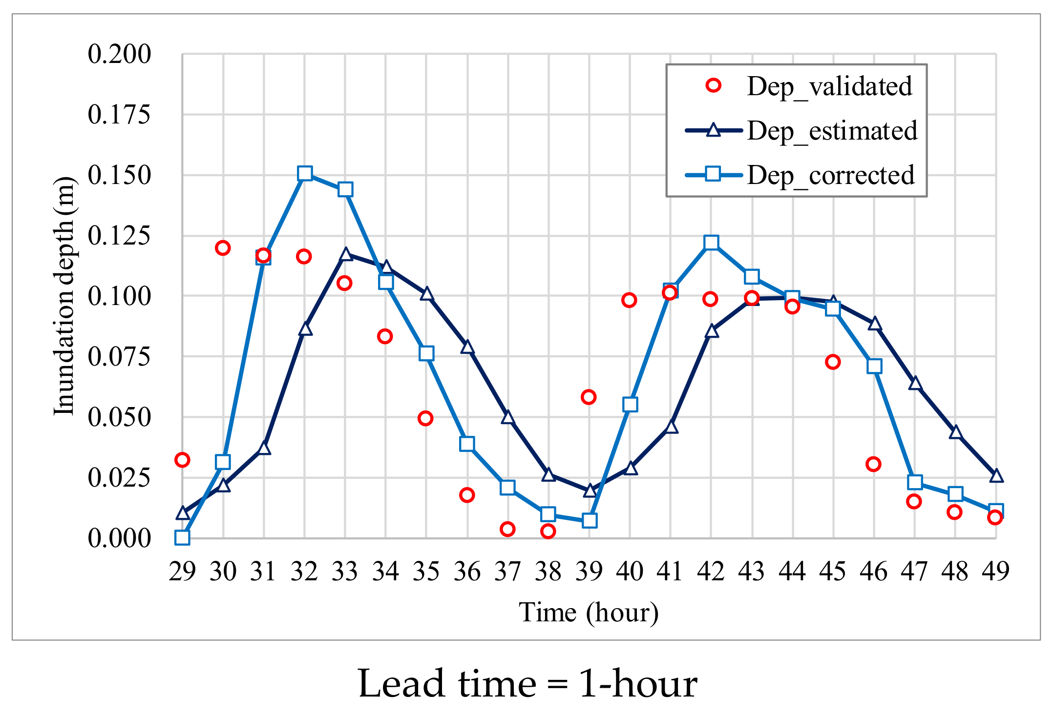
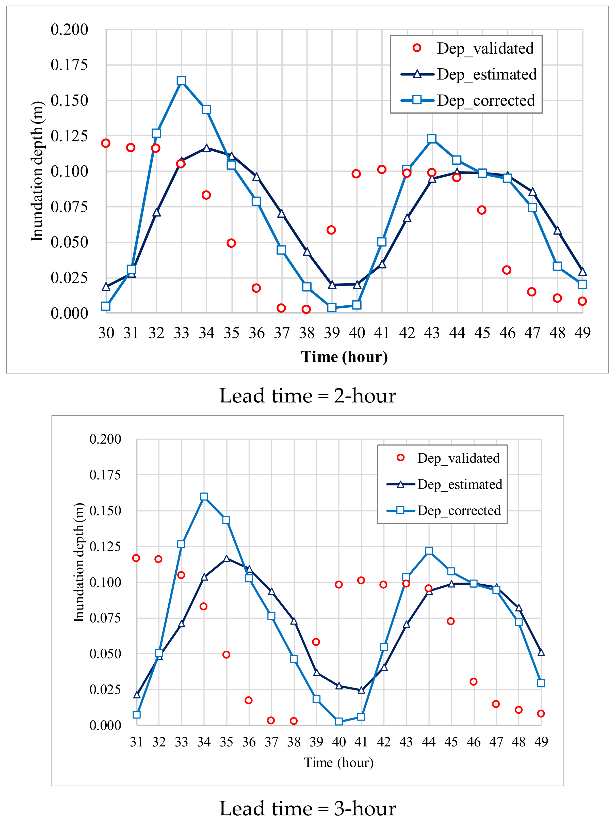
Accordingly, as for the 460th simulation case, the resulting inundation-depth estimates and associated 95% confidence intervals at the IoT sensor can be obtained from the SM_EID_IOT model as compared with the validated ones, as shown in Figure 14. It can be seen that the temporal change in the inundation-depth estimates at the three lead times resembles variation regarding the areal average rainfall in accordance with the high correlation. Moreover, at the 1 h lead time, the estimated inundation depths mostly lie around the 95% confidence interval, except for the 30th–31th and 40th–41th hour, where the inundation-depth estimates are about 0.119 m and 0.09 m, exceeding the upper bounds of 0.075 m and 0.085 m, respectively. Similar results can be found for the inundation-depth forecasts at the 2 h and 3 h lead times. The above results imply that the proposed SM_EID_IOT model can produce the inundation-depth estimate with high likelihood of approaching the true values (i.e., observations).

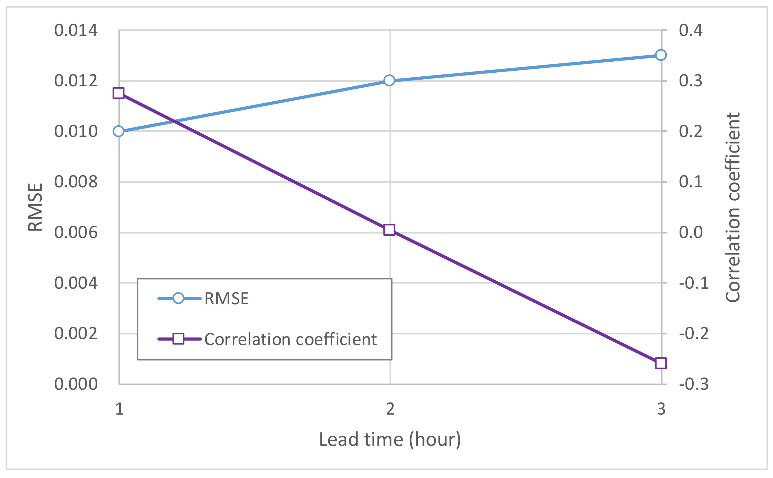
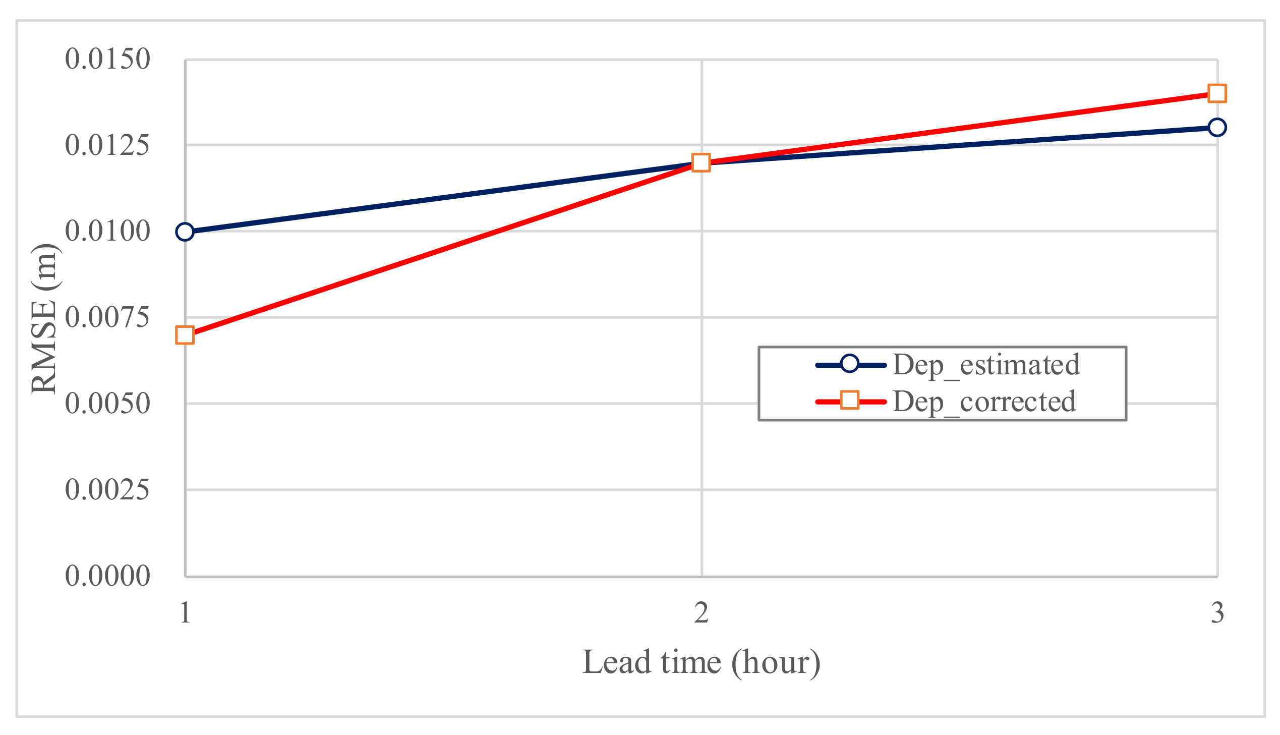
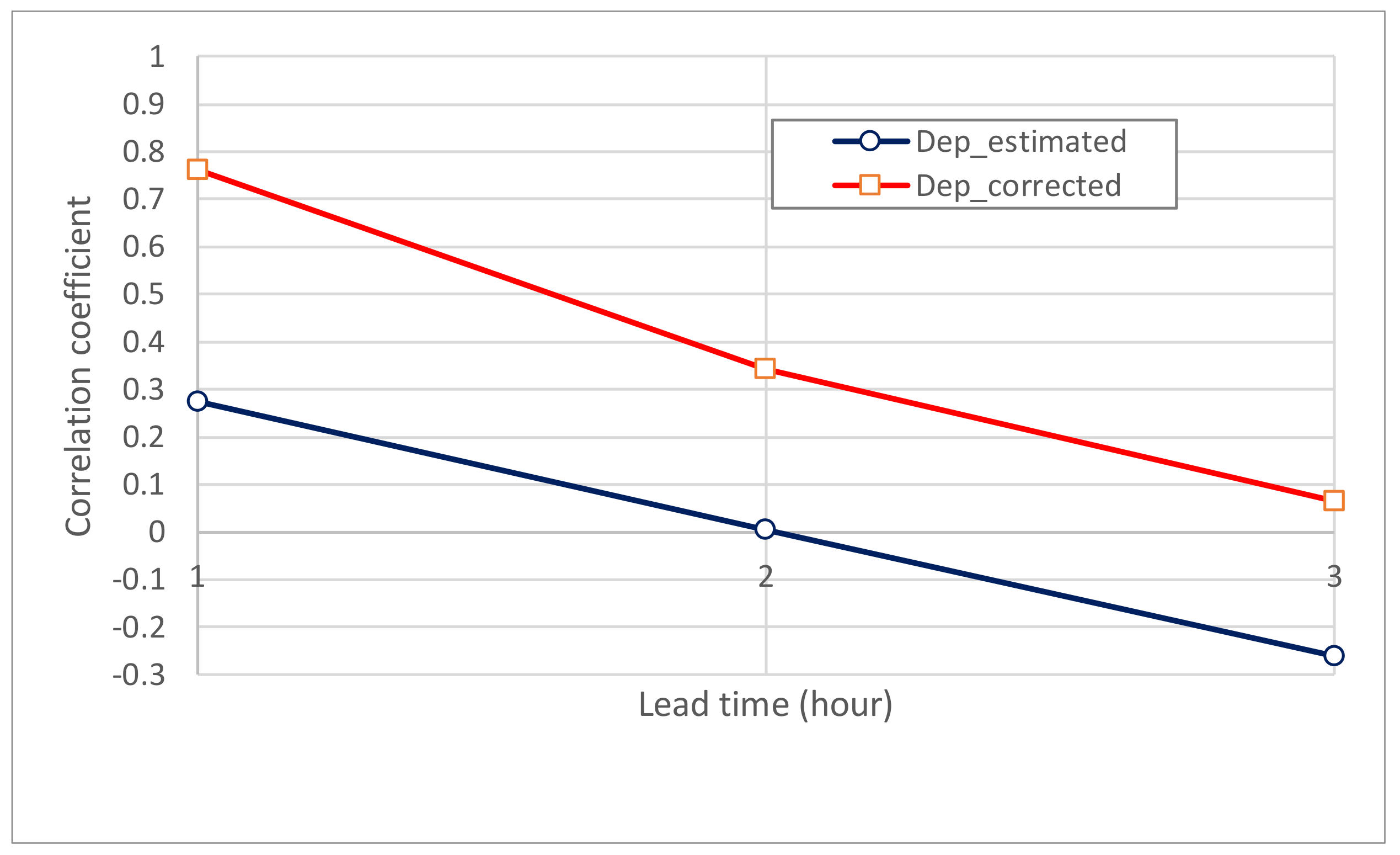
As can be seen in Figure 14, in spite of the proposed SM_EID_IOT model possibly producing reasonable inundation-depth estimates, the inundation-depth estimates at the 1 h lead time are underestimated as compared with the validated data at the 30th–32th hours regarding the 825th simulated event. Hence, to evaluate the accuracy of the inundation-depth forecasts at the various lead times, the performance in comparison with the estimated inundation depths and validated ones at the 31th–51th hours is carried out in terms of the root mean error (RMSE) and correlation coefficients, as shown in Figure 15. According to the results from Figure 15, the RMSE increases with the lead time; however, the correlation coefficient declines with the lead time. For example, although the estimations exhibit an obvious difference from the validation data in association with a large root mean error square (RMSE) (about 0.01 m), the corresponding correlation coefficient approaches 0.3, meaning the change in the average rainfall in time is close to that regarding the inundation depth; similar conclusions are also made based on the results from the 2 h and 3 h lead time. The above difference between the estimation and validations might be caused by the uncertainties in the observation and model parameters.

4.5.2. Real-Time Correction of Inundation-Depth Estimates

To facilitate the accuracy of the results from the proposed SM_EID_IOT model, the inundation-depth estimates are supposed to be adjusted based on the real-time measured data. The real-time error correction method is developed via the time series approach and Kalmen filtering equation (RTEC_TS&KF) [30]. Figure 16 and Figure 17 show the comparison between the validated, estimated, and corrected inundation depths, respectively, as well as the corresponding performance indices, respectively, indicating that the RMSE value increases with the lead time; in contrast, the correlation coefficient markedly decreases with the lead time. In spite of the RMSE values for the corrected inundation-depth estimates significantly increasing with the lead time, from 0.007 m to 0.014 m, on average, they are less than those for the forecasts (0.012 m). Moreover, with respect to the consistency wof the validations, the correlation coefficients for both inundation-depth estimations and corrections generally decrease with the lead time, 0.28–0.26 (estimations) and 0.74–0.06 (corrections), respectively. For illustration, the correlation coefficients for the corrections at the 1 h lead time approximate 0.7, obviously greater than that from the estimates (about 0.28). In particular, at the 3 h lead time with the worst correlation, −0.25 (estimations) and 0.07 (corrections), the corrections have better consistency with the validated datasets than the estimations. The above results reveal that the corrected inundation-depth forecasts exhibit better agreement with the observations than the underestimated/overestimated inundation-depth forecasts, with the marked errors even for the long lead times being able to be immediately adjusted.

In summary, the accuracy of the resulting inundation-depth estimates at various lead times (hours) from the proposed SM_EID_MTF with a reasonable reliability can be effectively improved based on the difference between the observations and estimates at the previous time steps during a rainfall-induced flooding event.

5. Conclusions

This study intends to propose a stochastic ANN-derived model for the estimation of the inundation depths at the roadside water-level sensors set up through the Internet of Things (IoT) (named the SM_EID_IOT). The proposed SM_EID_IOT is developed on the basis of the artificial neural network model ANN_GS-SA_MTF (Wu et al., 2021), in which the associated parameters are calibrated by means of the modified genetic algorithm (GA-SA) [30] under the consideration of multiple transfer functions. A basin located in northern Taiwan, the Nankan River watershed, is selected as the study area and the associated grid-based precipitation data regarding 20 historical rainstorms provided by Center Weather Bureau in Taiwan are utilized to reproduce 1000 simulations of the rainfall-induced inundations via as the training dataset for the development of the proposed SM_EID_IOT model.

According to the results from the correlation and sensitivity analysis, the inundation depths at the IoT sensor for the forward periods of 3 h (i.e., critical temporal resolution) and the corresponding precipitations at the neighboring grids within the specific distance of 3 km (i.e., critical spatial resolution) to the IoT sensor should be regarded as the uncertainty factors for the resulting inundation-depth estimate (i.e., model inputs) from the proposed SM_EID_IOT model. Additionally, the results from the model demonstration indicate that the validated inundation depths at the lead times of 3 h are almost located within the quantified 95% confidence intervals by the proposed SM_EID_IOT model, revealing that the proposed SM_EID_IOT can provide the inundation-depth estimates at the lead times of 3 h with a high likelihood of approaching the validated datasets. Furthermore, the corrected inundation-depth estimates by the real-time error correction method RTEC_TS&KF method integrated within the proposed SM_EID_IOT model could effectively improve the accuracy of the inundation-depth estimates by 50%; thereby, the estimate exhibits a good match with the validated datasets under a better temporal correlation (i.e., correlation coefficient approaching 0.8). Consequently, the proposed SM_EID_IOT model is capable of estimating more accurate inundation depths at the IoT sensors of interest with high reliability.

In addition to the estimation of the inundation depths at the particular locations at which the roadside water-level IoT sensors are set up, the rainfall-induced flooding map is necessarily delineated in order to primarily estimate the possible inundation area under conditions of the flood-rated indices, such as the flash-food potential index (FFPI) and flooding potential index (FPI) [48], and rainfall-rated variables, such as the radar precipitation [49,50]. As a result of the flooding map being composed of the gridded inundation depths, the inundation depths at the ungauged locations should be quantified; by doing so, future work would improve the application of the framework and detailed concepts of developing the proposed SM_EID_IOT model in the derivation of stochastic ANN-derived modeling (i.e., the ANN_GA-SA MTF model) for the inundation-depth estimates at the ungauged locations within the flood-prone zones.

References

- Wu, S.J.; Chang, C.H.; Hsu, C.T. Real-time error correction of two-dimensional flood-inundation simulations during rainstorm events. Stoch. Environ. Res. Risk Assess. 2020, 34, 641–667. [Google Scholar] [CrossRef]
- Amarnath, G. An algorithm for rapid flood inundation mapping from optical data using a reflectance differencing technique. J. Risk Manag. 2014, 7, 239–250. [Google Scholar] [CrossRef]
- Park, I.; Seong, H.; Ryu, Y.; Rhee, D.S. Measuring inundation depth in a subway station using the laser image analysis method. Water 2018, 10, 1558. [Google Scholar] [CrossRef] [Green Version]
- Chen, A.S.; Hsu, M.H.; Teng, W.H.; Huang, C.J.; Yeh, S.H.; Ien, W.Y. Establishment the Database of Inundation Potential in Tawian. Nat. Hazards 2018, 377, 107–132. [Google Scholar]
- Rebolho, C.; Andreassian, V.; Moine, N.L. Inundation mapping based on reach-scale effective geometric. Hydrol. Earth Syst. Sci. Discuss. 2018, 22, 5967–5985. [Google Scholar] [CrossRef] [Green Version]
- Ongdas, N.; Akiyanova, F.; Karakulov, Y.; Muratbayeva, A.; Zinabdin, N. Application of HEC-RAS (2D) for Flood Hazard Maps Generation for Yesil (Ishim) River in Kazakhstan. Water 2020, 12, 2672. [Google Scholar] [CrossRef]
- Fohringer, J.; Dransch, D.; Kreibich, H.; Schröter, K. Social media as an information source for rapid flood inundation mapping. Nat. Hazards Earth Syst. Sci. 2015, 15, 2725–2738. [Google Scholar] [CrossRef] [Green Version]
- Assumpção, T.H.; Popescu, I.; Jonoski, A.; Solomatine, D.P. Citizen observations contributing to flood modelling: Opportunities and challenges. Hydrol. Earth Syst. Sci. 2018, 22, 1473–1489. [Google Scholar] [CrossRef] [Green Version]
- Chang, L.C.; Mohd Zaki, M.A.; Yang, S.N.; Chang, F.J. Building ANN-Based Regional Multi-Step-Ahead Flood Inundation Forecast Models. Water 2018, 10, 1283. [Google Scholar] [CrossRef] [Green Version]
- Yang, S.N.; Chang, L.C. Regional inundation forecasting using machine learning techniques with the Internet of Thing. Water 2020, 12, 1578. [Google Scholar] [CrossRef]
- Jung, Y.J.; Kim, D.K.; Kim, D.W.; Kim, M.; Lee, S.O. Simplified Flood Inundation Mapping Based on Flood Elevation-Discharge Rating Curves Using Satellite Images in Gauged Watersheds. Water 2014, 6, 1280–1299. [Google Scholar] [CrossRef]
- Shastry, A.; Durand, M. Utilizing Flood Inundation Observations to Obtain Floodplain Topography in Data-Scarce Regions. Front. Earth Sci. 2019, 6, 243. [Google Scholar] [CrossRef] [Green Version]
- Jain, S.K.; Mani, P.M.; Jain, S.K.; Prakash, P.; Singh, V.P.; Tullos, D.; Kumar, S.; Agarwal, S.P.; Dimri, A.P. A brief review of flood forecasting techniques and their applications. Int. J. River Basin Manag. 2018. [Google Scholar] [CrossRef]
- Myronidis, D.; Ivanova, E. Generating regional models for estimating the peak flows and environmental flows magnitude for the Bulgarian-Greek Rhodope mountain range torrential watersheds. Water 2020, 12, 784. [Google Scholar] [CrossRef] [Green Version]
- Paschalis, A.; Molnar, P.; Fatichi, S.; Burlando, O. A stochastic model for high-resolution space-time precipitation simulation. Water Resour. Res. 2013, 49, 8400–8417. [Google Scholar] [CrossRef]
- Ran, Q.; Hong, Y.; Li., W.; Gao, J. A modeling study of rainfall-induced shallow landslide mechanisms under different rainfall characteristics. J. Hydrol. 2018, 363, 790–801. [Google Scholar] [CrossRef]
- Kan, G.; He, X.; Li, J.; Ding, L.; Hong, Y. Computer aided numerical methods for hydrological model calibration: An overview and recent development. Arch. Comput. Methods Eng. 2019, 26, 35–59. [Google Scholar] [CrossRef]
- Wu, S.J.; Hsu, C.T.; Chang, C.H. Stochastic modeling of artificial neural networks for real-Time hydrological forecasts based on uncertainties in transfer Functions and ANN weights. Hydrol. Res. 2021. [Google Scholar] [CrossRef]
- Gupta, H.V.; Beven, K.J.K.; Wagener, T. Model calibration and uncertainty estimation. In Encyclopedia of Hydrologic Sciences; Anderson, M.G., Ed.; Wiley: Chichester, UK, 2005. [Google Scholar]
- Melsen, L.; Teuling, A.; Torfs, P.; Zappa, M.; Mizukami, N.; Clark, M.; Uijlenhoet, R. Representation of spatial and temporal variability in large-domain hydrological models: Case study for a mesoscale pre-Alpine basin. Hydrol. Earth Syst. Sci. 2016, 29, 2207–2226. [Google Scholar] [CrossRef] [Green Version]
- Campolo, M.; Andreussi, P.; Soldati, A. River flood forecasting with a neural network model. Water Resour. Res. 1999, 35, 1191–1197. [Google Scholar] [CrossRef]
- Wang, L.; Zeng, Y.; Chen, T. Back propagation neural network with adaptive differential evolution algorithm for time series forecasting. Expert Syst. Appl. 2015, 42, 855–863. [Google Scholar] [CrossRef]
- Ioannou, K.; Myronidis, D.; Lefakis, P.; Stathis, D. The use of artificial neural networks (ANNs) for the forecast of precipitation levels of lake Doirani (N. Greece). Fresenius Environ. Bull. 2010, 19, 1921–1927. [Google Scholar]
- Chang, L.C.; Shen, H.Y.; Chang, F.J. Regional flood inundation nowcast using hybrid SOM and dynamic neural networks. J. Hydrol. 2014, 519, 476–489. [Google Scholar] [CrossRef]
- Sung, J.Y.; Lee, J.; Chung, I.W.; Heo, J.H. Hourly Water Level Forecasting at Tributary Affected by Main River Condition. Water 2017, 6, 644. [Google Scholar] [CrossRef] [Green Version]
- Chang, L.C.; Chang, F.J.; Yang, S.N.; Kao, I.F.; Ku, Y.Y.; Kuo, C.L.; Ir. Mohd Zaki bin Mat Amin; Building an Intelligent Hydroinformatics Integration Platform for Regional Flood Inundation Warning Systems. Water 2019, 11, 9. [Google Scholar] [CrossRef] [Green Version]
- Shamseldin, A.Y. Artificial neural network model for river flow forecasting in a developing country. J. Hydroinform. 2010, 12, 22–35. [Google Scholar] [CrossRef] [Green Version]
- Tamiru, H.; Dinka, M.O. Application of ANN and HEC-RAS model for flood simulation mapping in lower Baro Akobo River Basin, Ethiopia. J. Hydrol. Reg. Stud. 2021, 36, 100855. [Google Scholar] [CrossRef]
- Wu, S.J.; Lien, H.C.; Chang, C.H. Calibration of a conceptual rainfall-runoff model using a genetic algorithm integrated with runoff estimation sensitivity to parameters. J. Hydroinformatics 2012, 14, 497–511. [Google Scholar] [CrossRef]
- Wu, S.J.; Lien, H.C.; Chang, C.H.; Shen, J.C. Real-Time Correction of Water Stage Forecast during Rainstorm Events Using Combination of Forecast Errors. Stoch. Environ. Res. Risk Assess. 2012, 26, 519–531. [Google Scholar] [CrossRef]
- Wu, S.J.; Hsu, C.T.; Chang, C.H. Stochastic modeling of gridded short-term rainstorms. Hydrol. Res. 2021, 52, 876–904. [Google Scholar] [CrossRef]
- Deltares Systems. SOBEK User Manual. Delft, the Netherlands. 2014. Available online: http://content.oss.deltares.nl/delft3d/manuals/SOBEK_User_Manual.pdf (accessed on 22 October 2021).
- Nataf, A. Determination des distributions don’t les marges sontdonnees. C. R. L’acad. Sci. 1962, 225, 42–43. [Google Scholar]
- Liu, P.L.; Der Kiureghian, A. Multivariate distribution models with prescribed marginals covariances. Probabilistic Eng. Mech. 1986, 1, 105–112. [Google Scholar] [CrossRef]
- Hydraulic Institute DHI. MIKE 11: A Modelling System for Rivers and Channels, Reference Manual; Danish Hydraulic Institute: Lakewood, CO, USA, 2016. [Google Scholar]
- Danish Hydraulic Institute DHI. MIKE 21: Flow Model FM, Hydrodynamic Module Reference Manual; Danish Hydraulic Institute: Lakewood, CO, USA, 2019. [Google Scholar]
- Horritt, M.D. Establishment the Datatbase of Inundation Potential in Tawian Bates, P.D. Predicting floodplain inundation: Raster-based modelling versus the finite-element approach. Hydrol. Process. 2001, 18, 825–842. [Google Scholar] [CrossRef]
- Imrie, C.; Durucan, S.; Korre, A. River flow prediction using artificial neural networks: Generalization beyond the calibration range. J. Hydrol. 2000, 233, 138–153. [Google Scholar] [CrossRef]
- Maca, P.; Pech, P.; Pavlasek, J. Comparing the Selected Transfer Functions and Local Optimization Methods for Neural Network Flood Runoff Forecast. Math. Probl. Eng. 2014, 2014, 782351. [Google Scholar] [CrossRef] [Green Version]
- Dawson, C.W.; Wilby, R.L. Hydrological modelling using artificial neural networks. Prog. Phys. Geogr. 2001, 25, 80–108. [Google Scholar] [CrossRef]
- Li, J.Y.; Chow, T.W.S.; Yu, Y.L. Estimation theory and optimization algorithm for the number of hidden units in the higher-order feedforward neural network. In Proceedings of the IEEE International Conference on Neural Networks, Perth, WA, Australia, 27 November–1 December 1995; Volume 3, pp. 1229–1233. [Google Scholar]
- Zhang, Z.; Ma, X.; Yang, Y. Bounds on the number of hidden neurons in three-layer binary neural networks. Neural Netw. 2003, 16, 995–1002. [Google Scholar] [CrossRef]
- Shibata, K.; Ikeda, Y. Effect of number of hidden neurons on learning in large-scale layered neural networks. In Proceedings of the ICROS-SICE International Joint Conference (ICCAS-SICE ’09), Fukuoka, Japan, 18–21 August 2009; pp. 5008–5013. [Google Scholar]
- Hunter, D.; Yu, H.; Pukish, M.S.; Kolbusz, J.B.M.; Wilamowski, B.M. Selection of proper neural network sizes and architectures: A comparative study. IEEE Trans. Ind. Inform. 2012, 8, 228–240. [Google Scholar] [CrossRef]
- Sheela, K.; Deepa, S.N. Review on Methods to Fix Number of Hidden Neurons in Neural Networks. Math. Probl. Eng. 2013. [Google Scholar] [CrossRef] [Green Version]
- Yang, J.C.; Tung, Y.K. Establishment of flow-duration curve and the assessment of its certainty. In Final Report of Environment Protection Agency; Environment Protection Agency: Taipei City, Taiwan, 1996. [Google Scholar]
- Terink, W.; Leijnse, H.; Eertwegh, G.V.D.; Uijlenhoet, R. Spatial resolutions in areal rainfall estimation and their impact on hydrological simulations of a lowland catchment. J. Hydrol. 2018, 563, 319–335. [Google Scholar] [CrossRef]
- Zaharia, L.; Costache, R.; Pravalie, R.; Ioana-Toroimac, G. Mapping flood and flooding potential indices: A methodological approach to identifying areas susceptible to flood and flooding risk-Case study: The Prahova catchment (Romania). Front. Earth Sci. 2017, 11, 229–274. [Google Scholar] [CrossRef]
- Shen, X.Y.; Wang, D.C.; Mao, K.B.; Anagnostou, E.; Hong, Y. Inundation extent mapping by synthetic aperture radar: A review. Remote Sens. 2019, 11, 879. [Google Scholar] [CrossRef] [Green Version]
- Try, S.; Tanaka, S.; Tanaka, K.; Sayama, T.; Oeurng, C.; Uk, S. Comparison of gridded precipitation datasets for rainfall-runoff and inundation modeling in the Mekong River Basin. PLoS ONE 2020, 15, e0226814. [Google Scholar] [CrossRef] [Green Version]
Figure 1.
Graphical process of extracting the gridded rainfall characteristics from observed hyetographs of rainstorm events [31]).
Figure 2.
Graphical process of combining the simulated gridded rainfall characteristics as the gridded rainstorms [31].
Figure 3.
Graphic framework of developing and applying the ANN_GA-SA_MTF model [18].
Figure 4.
Locations and DEM as well as QPE grids (blue circle) within the study area, Nankan River watershed (yellow region) [18].
Figure 5.
Hyetographs of 20 observed rainstorm events used in the model development and application [18].
Figure 6.
2D SOBEK model for the study area (Nankan River watershed) (note: the circle is the rainfall-runoff computing node for each sub-basin).
Figure 7.
Flooding risk map and locations of potential inundated spots within the study area (the Nankan River watershed).
Figure 8.
Relationship between the inundation depth and associated areal average of rainfall calculated using the simulated gridded rainfall with the specific distances from the IoT sensor of interest.
Figure 9.
Correlation coefficients and associated statistical properties of inundation depths with the areal average rainfall calculated using the simulated gridded rainfall with specific distances from the IoT sensor of interest.
Figure 10.
The averages of absolute sensitivity coefficients regarding the areal average rainfall and inundation depths at the various forward time steps.
Figure 11.
Summary for the estimation of the number of hidden neurons via various methods.
Figure 12.
Summary of the weights of the transfer function for calculating the weighted average of inundation-depth estimates.
Figure 13.
Relationship between the areal average rainfall and inundation depths regarding the 825th validated rainfall-induced flood event.
Figure 14.
Comparison among the validated, estimated, and corrected inundation depths as well as the quantified 95% confidence intervals for the validated rainfall-induced flood event by the proposed SM_EID_IOT model.
Figure 15.
Summary of the performance indices of the inundation-depth estimates and comparison with the validation datasets at various lead times.
Figure 16.
Comparison among the validated inundation depths and the corrected as well as corrected ones by the proposed SM_EID_IOT model during the validated rainfall-induced flood event.
Figure 17.
Summary of the performance indices of the inundation-depth estimates and the corresponding corrections for the validated rainfall-induced flood event.