
Groundwater Level Prediction Using a Multiple Objective Genetic Algorithm-Grey Relational Analysis Based Weighted Ensemble of ANFIS Models

 , ,
, ,  , ,
, ,  , and
, and
Abstract
:1. Introduction
2. Methodology
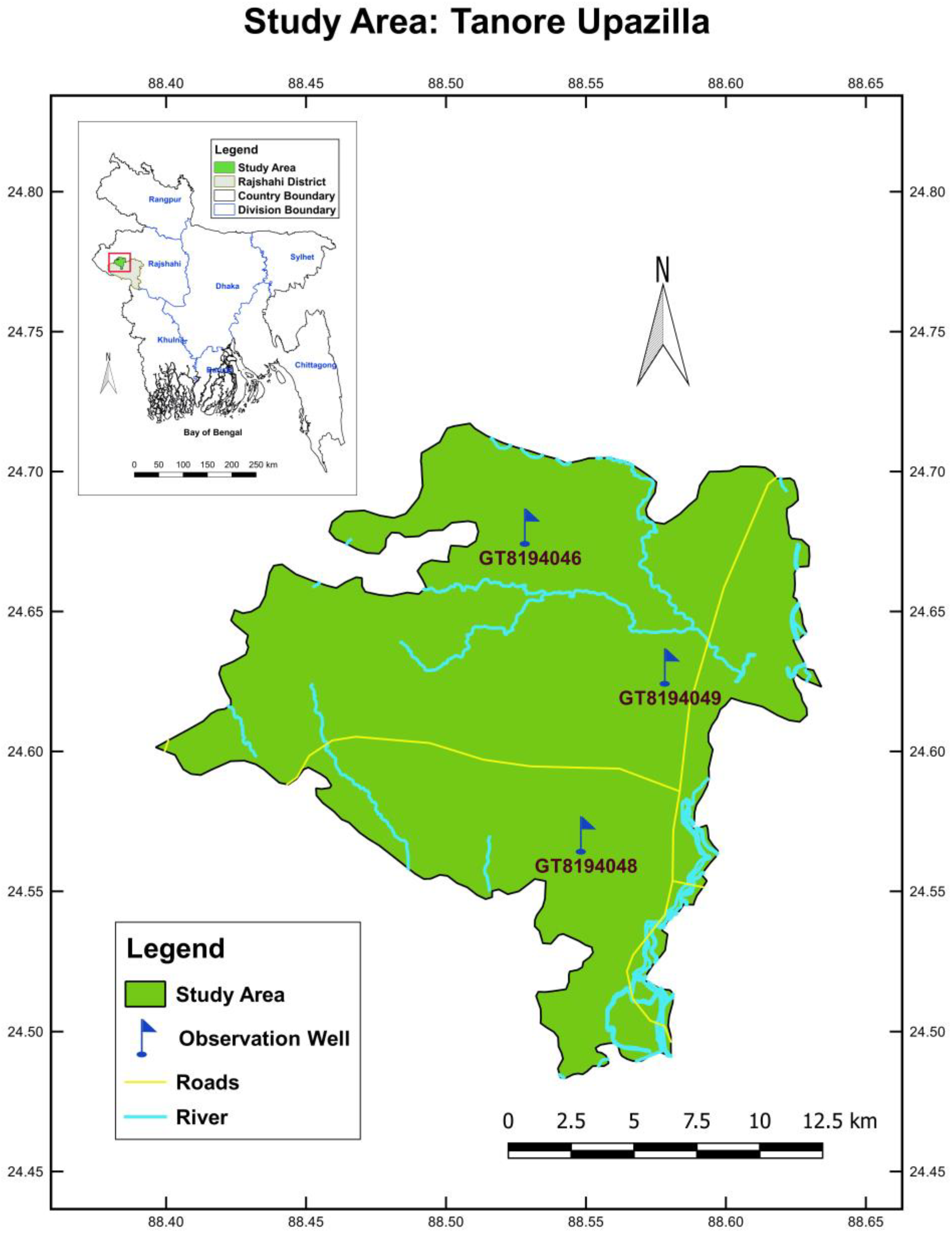
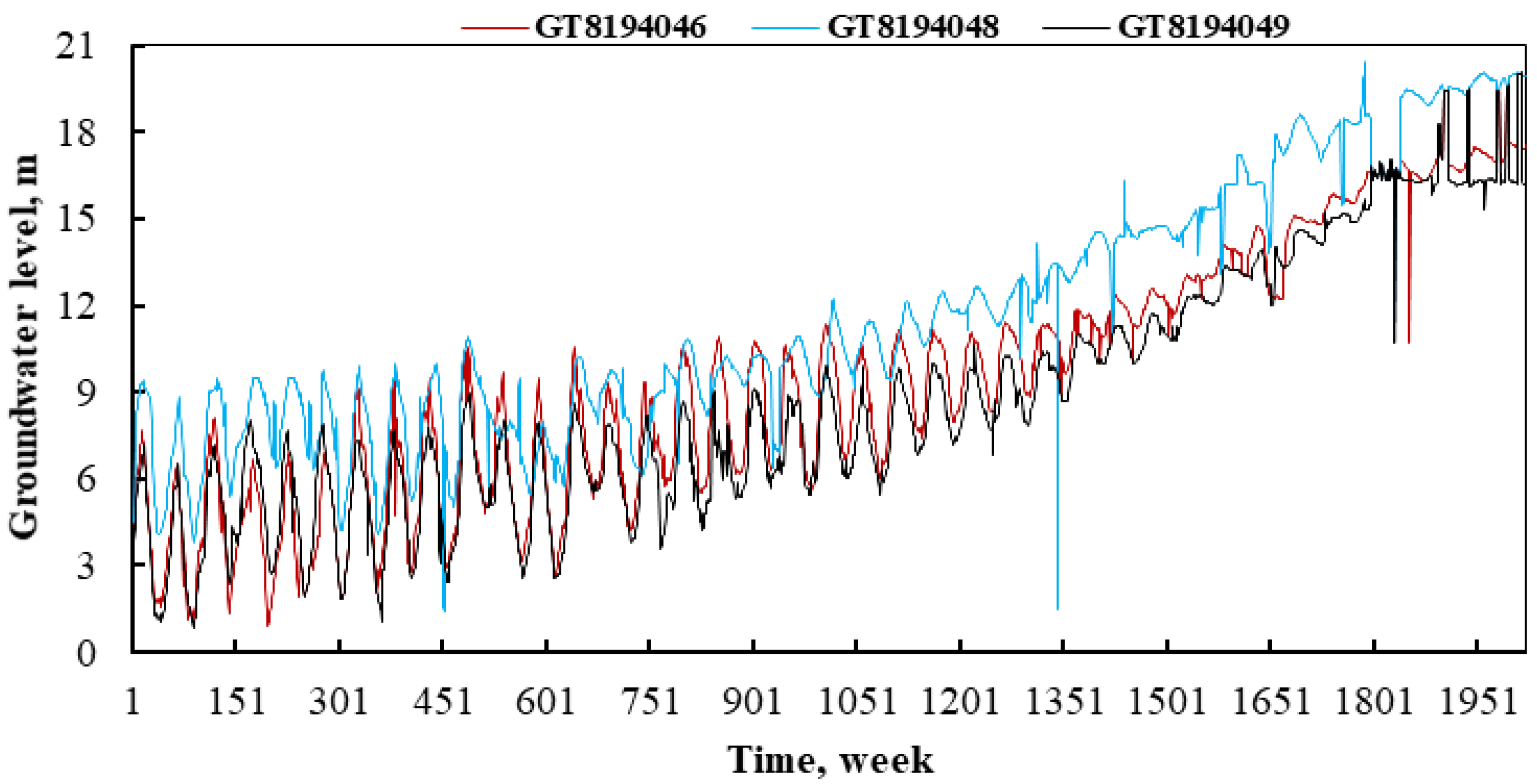
2.1. Study Area and the Data
2.1.1. Missing Value Imputation
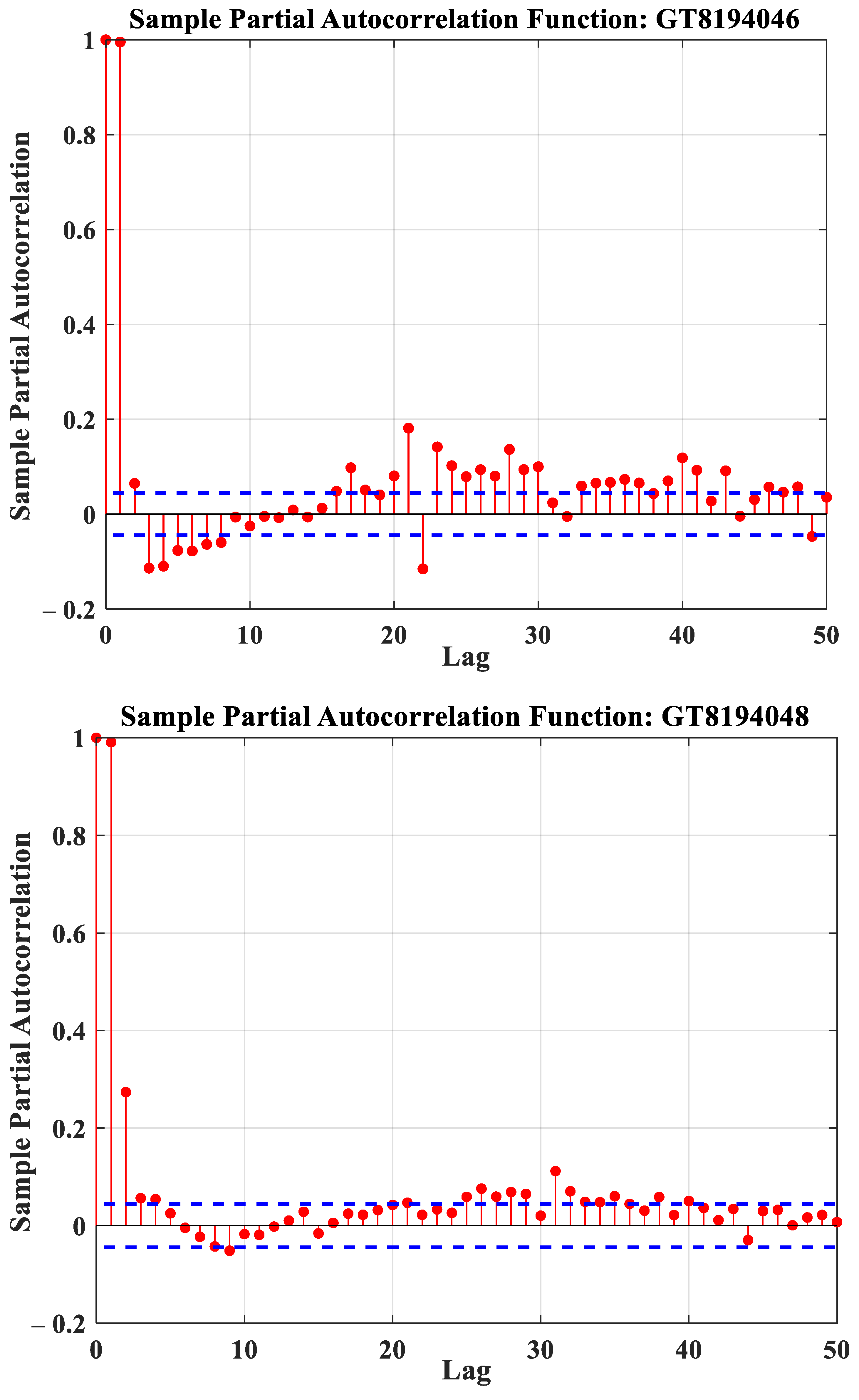
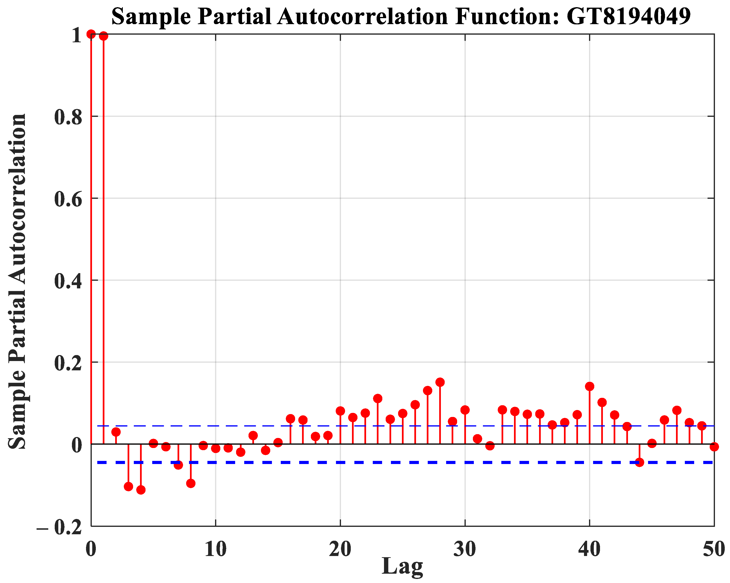
2.1.2. Selection of Input Variables
- Partial autocorrelations (PACF)
- 2.
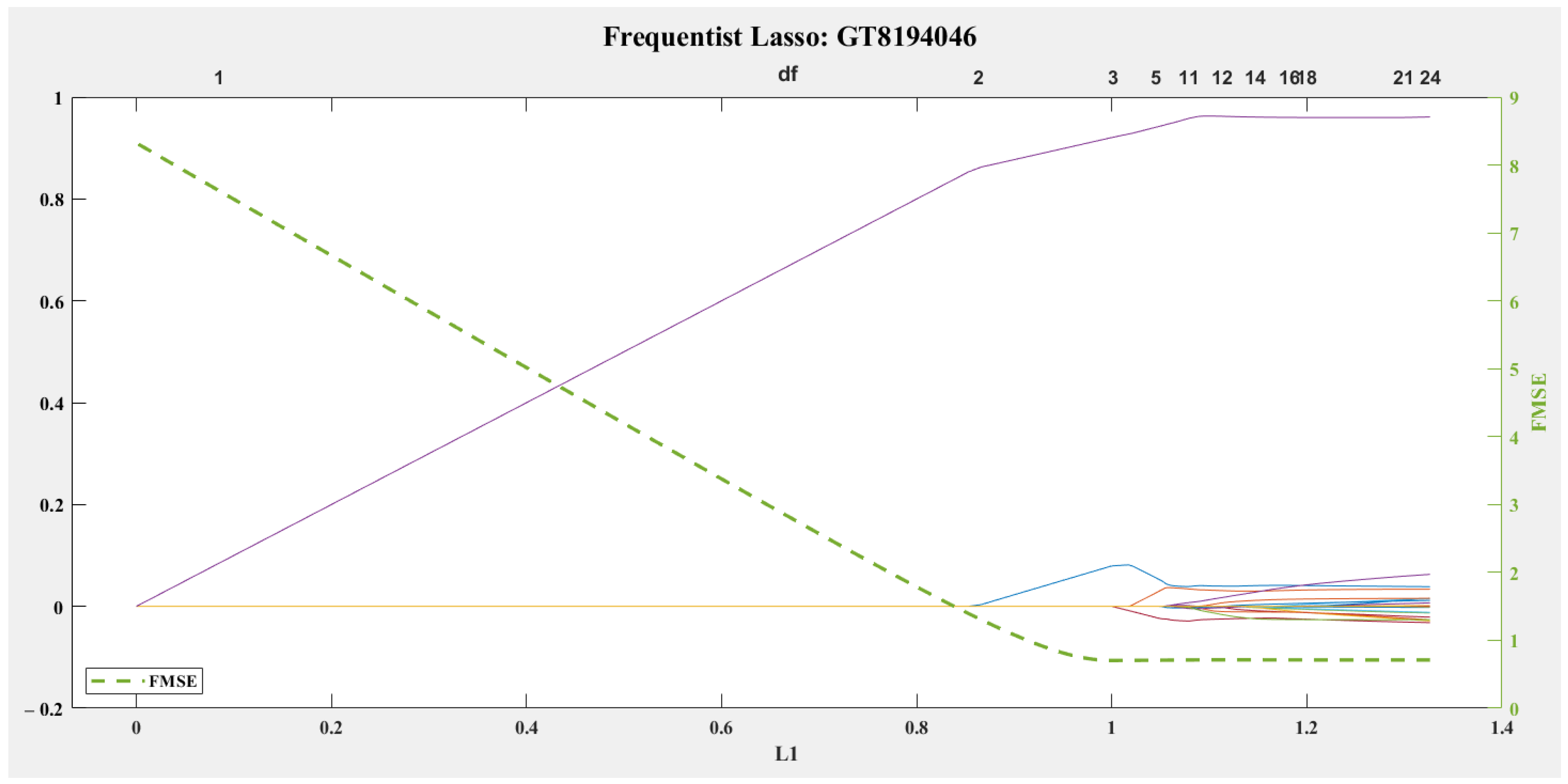
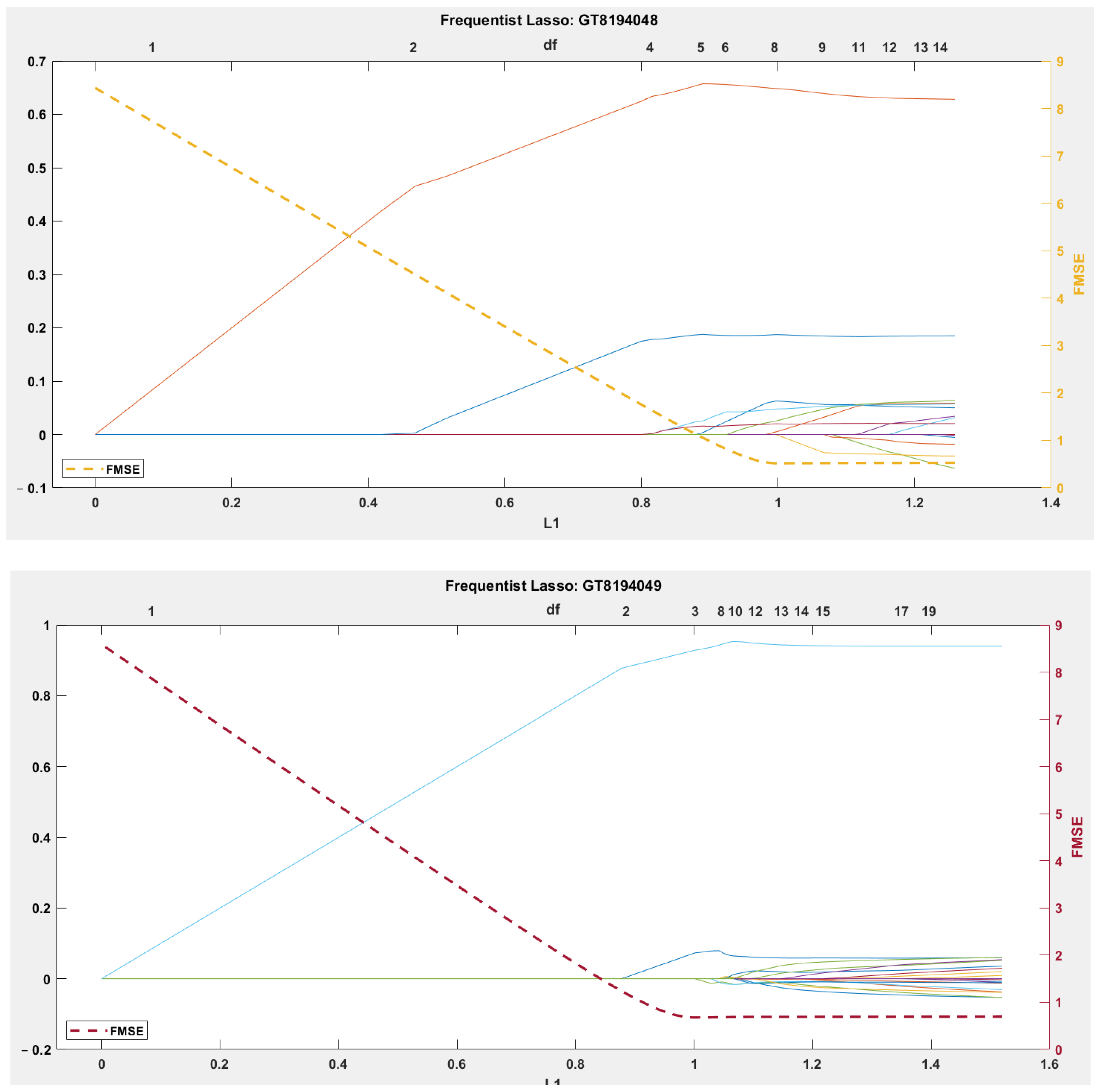
- Frequentist Lasso Regression (FLR)
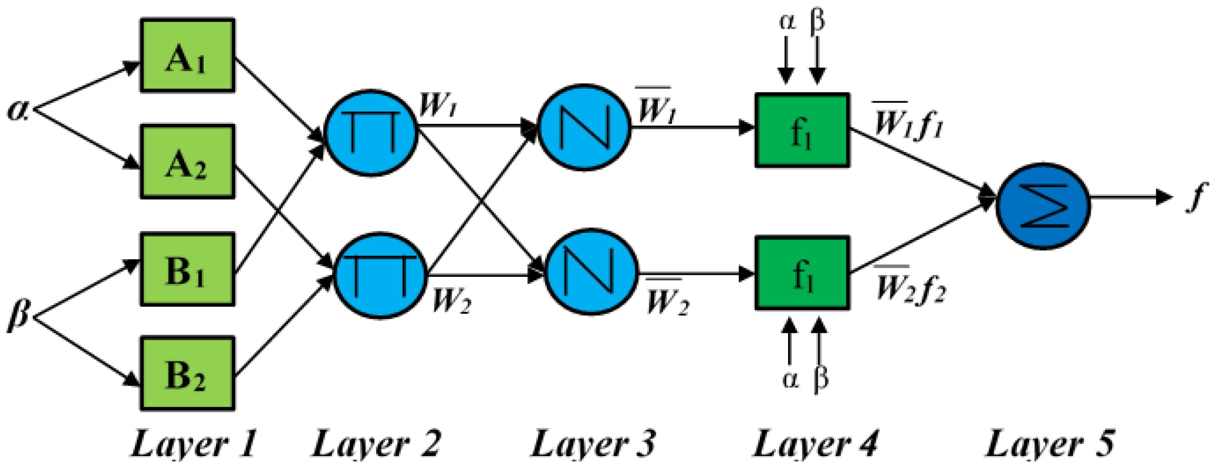
2.2. Prediction Model: Adaptive Neuro Fuzzy Inference System (ANFIS)
2.3. Algorithms to Tune ANFIS Parameters
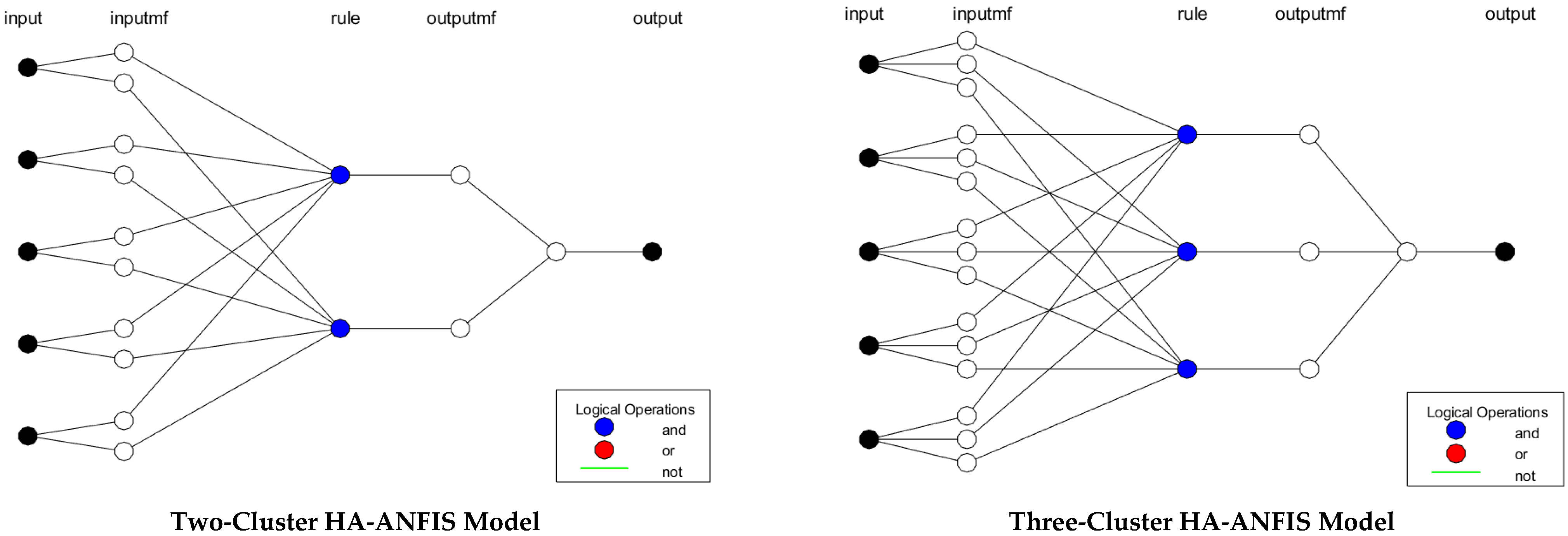
2.3.1. Hybrid Algorithm (HA)
2.3.2. Differential Evolution (DE)
2.3.3. Particle Swarm Optimization (PSO)
2.4. Developed ANFIS Models
2.5. Training of Optimized ANFIS Models
2.6. Weight Calculation
2.7. Ensemble Prediction
3. Results and Discussion
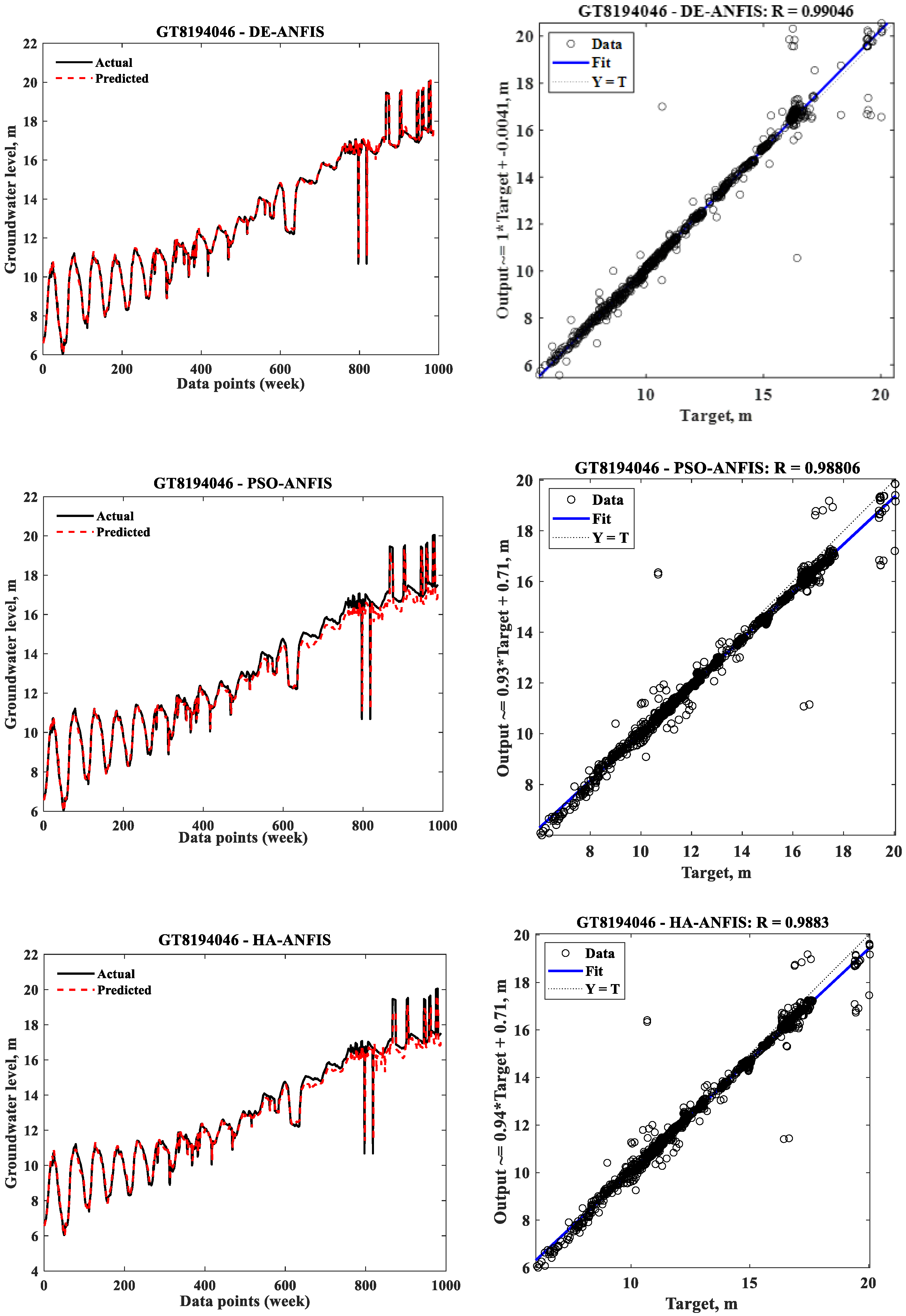
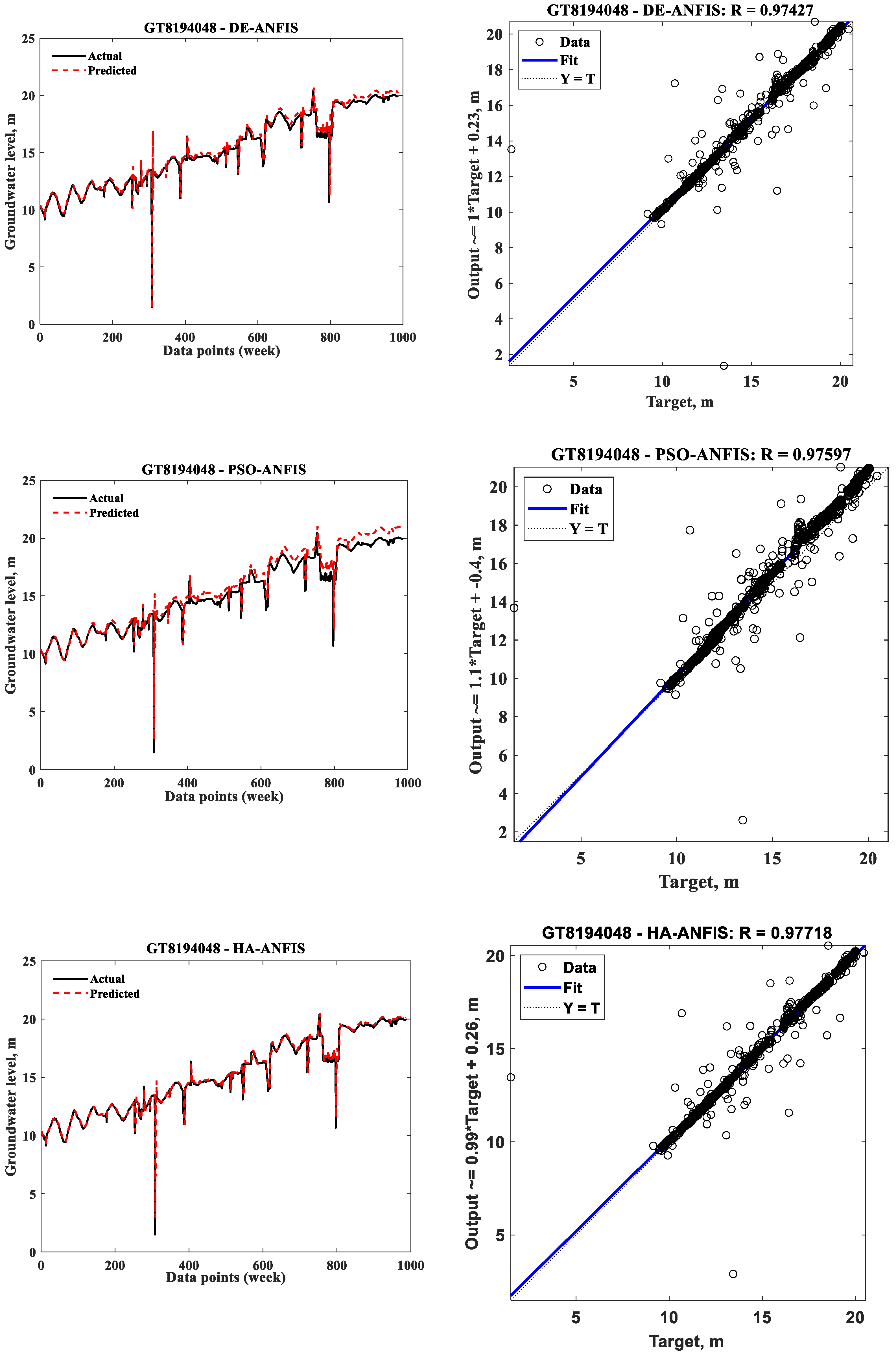
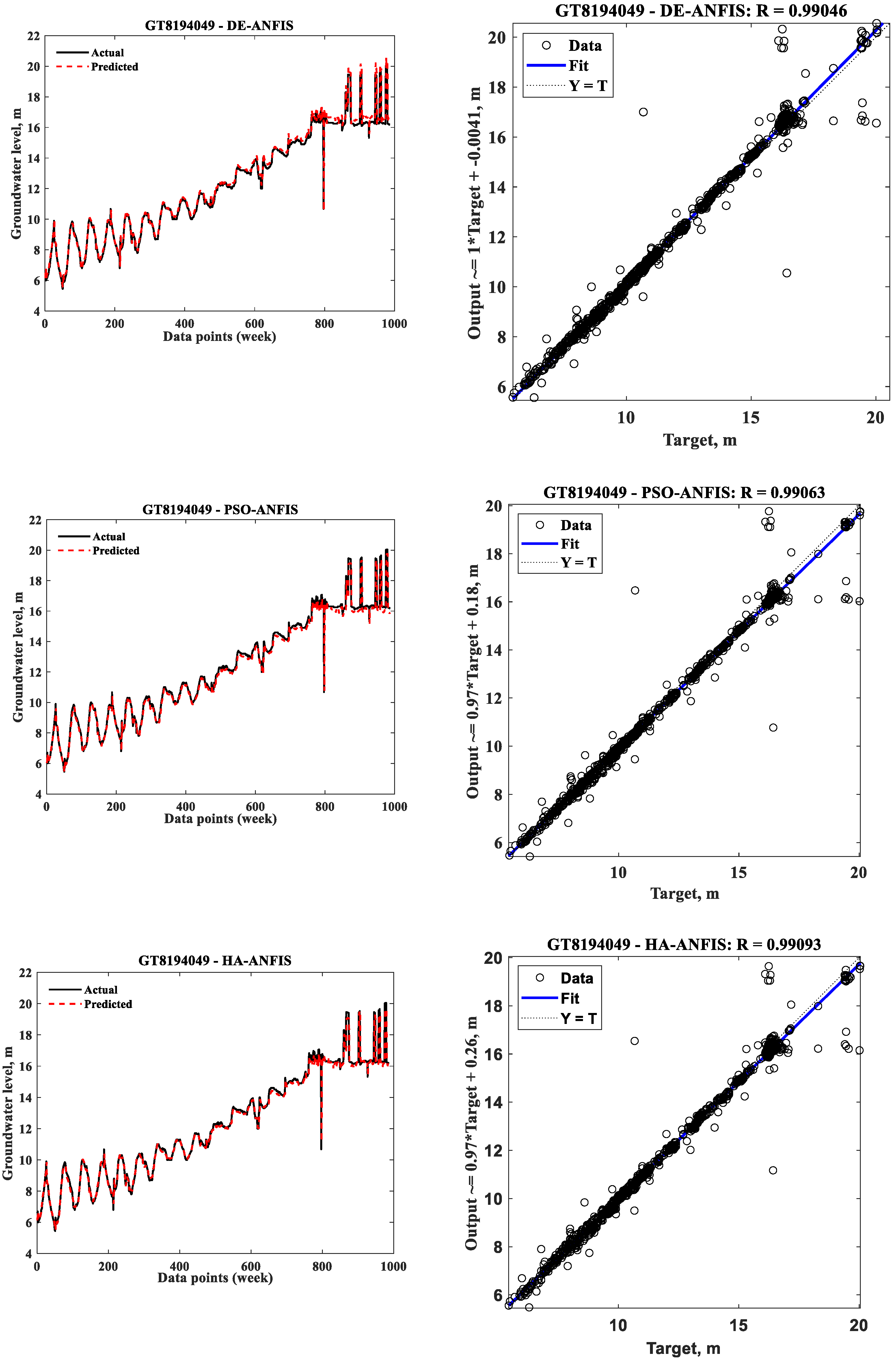
3.1. Prediction of Individual Models
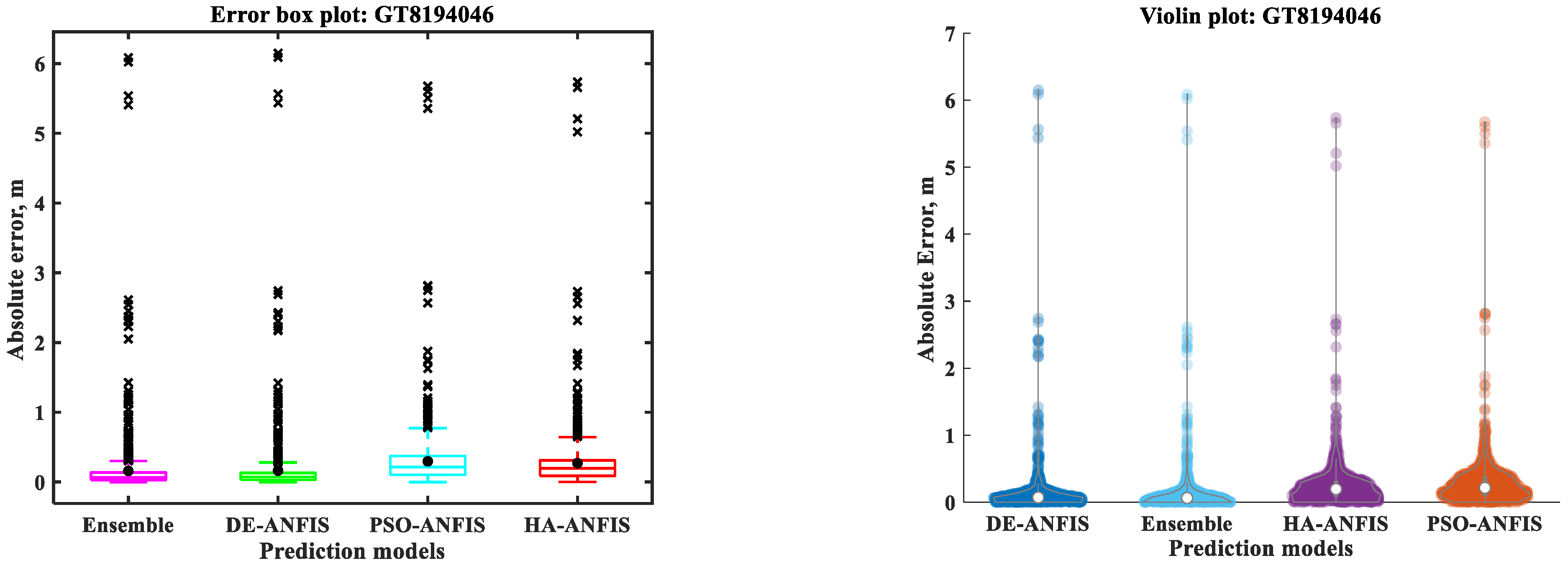
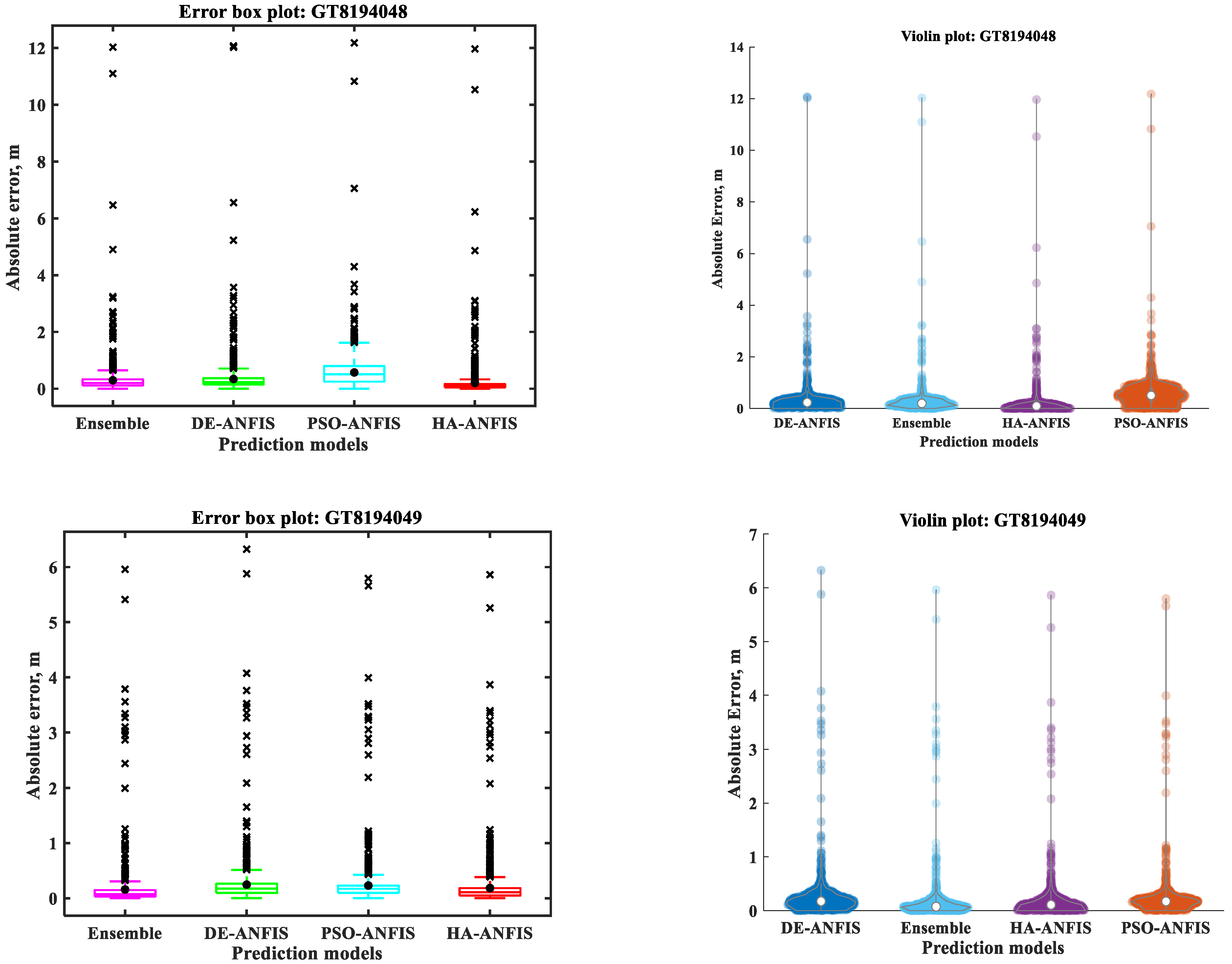
3.2. Ensemble Prediction
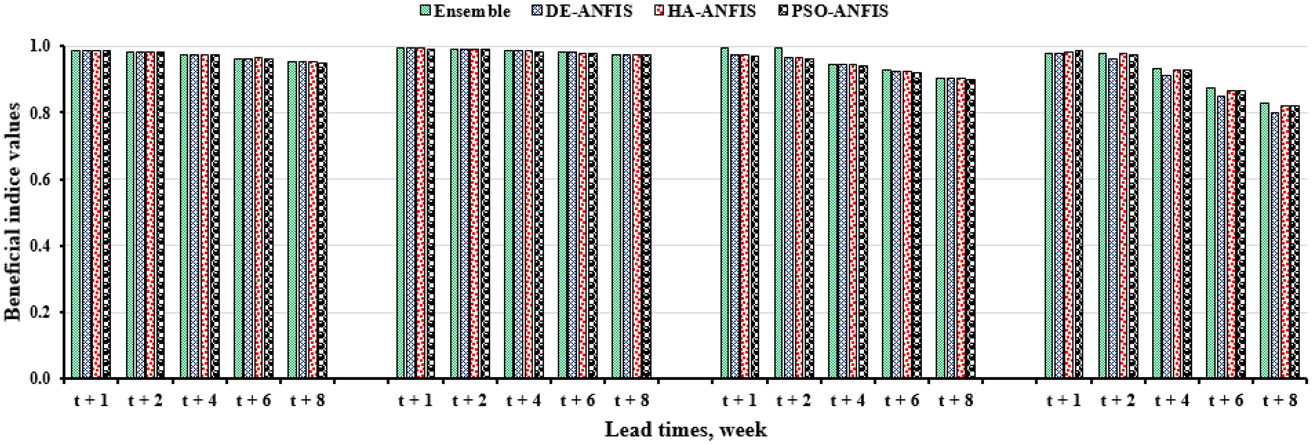
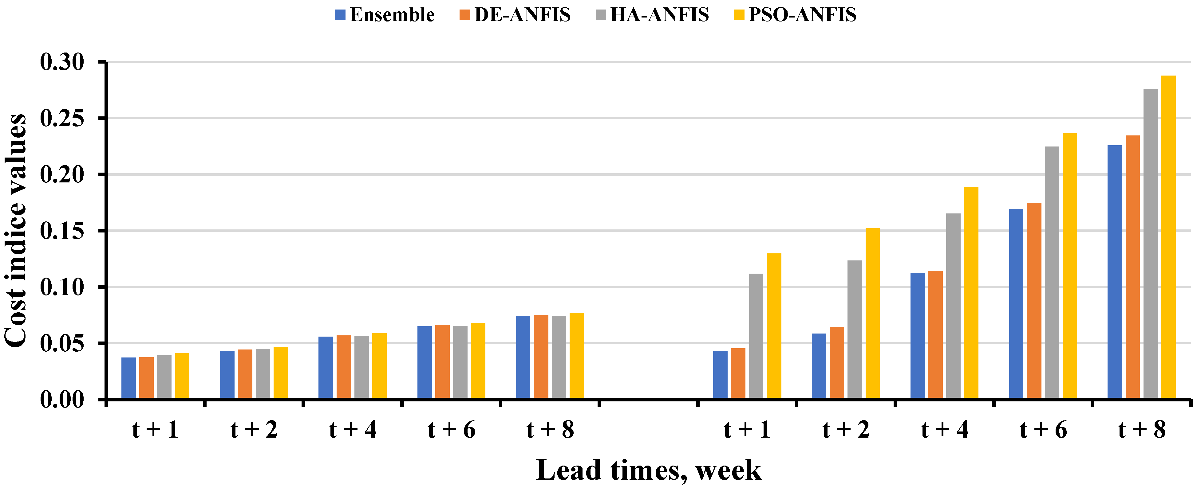
4. Performance Comparison of the Prediction Models for Forecasting 2-, 4-, 6-, and 8-Week Ahead Groundwater Level Fluctuations
5. Conclusions
Author Contributions
Funding
Institutional Review Board Statement
Informed Consent Statement
Data Availability Statement
Acknowledgments
Conflicts of Interest
Appendix A
Appendix A.1. Performance Evaluation Indexes
Appendix A.2. Ranking of the Prediction Models Using Shannon’s Entropy
References
- Wada, Y.; Bierkens, M.F.P. Sustainability of global water use: Past reconstruction and future projections. Environ. Res. Lett. 2014, 9, 104003. [Google Scholar] [CrossRef]
- Hoque, M.A.; Adhikary, S.K. Prediction of groundwater level using artificial neural network and multivariate time series models. In Proceedings of the 5th International Conference on Civil Engineering and Sustainable Development (ICCESD 2020), Khulna, Bangladesh, 7–9 February 2020; pp. 1–8. [Google Scholar]
- Doble, R.C.; Pickett, T.; Crosbie, R.S.; Morgan, L.K.; Turnadge, C.; Davies, P.J. Emulation of recharge and evapotranspiration processes in shallow groundwater systems. J. Hydrol. 2017, 555, 894–908. [Google Scholar] [CrossRef]
- Masterson, J.P.; Garabedian, S.P. Effects of sea-level rise on ground water flow in a coastal aquifer system. Groundwater 2007, 45, 209–217. [Google Scholar] [CrossRef] [PubMed]
- Park, E.; Parker, J.C. A simple model for water table fluctuations in response to precipitation. J. Hydrol. 2008, 356, 344–349. [Google Scholar] [CrossRef]
- Fahimi, F.; Yaseen, Z.M.; El-shafie, A. Application of soft computing based hybrid models in hydrological variables modeling: A comprehensive review. Theor. Appl. Climatol. 2017, 128, 875–903. [Google Scholar] [CrossRef]
- Govindaraju, R.S. Artificial neural networks in hydrology. I: Preliminary concepts. J. Hydrol. Eng. 2000, 5, 115–123. [Google Scholar] [CrossRef]
- Govindaraju, R.S. Artificial neural networks in hydrology. II: Hydrologic applications. J. Hydrol. Eng. 2000, 5, 124–137. [Google Scholar]
- Maier, H.R.; Jain, A.; Dandy, G.C.; Sudheer, K.P. Methods used for the development of neural networks for the prediction of water resource variables in river systems: Current status and future directions. Environ. Model. Softw. 2010, 25, 891–909. [Google Scholar] [CrossRef]
- Sadler, J.M.; Goodall, J.L.; Morsy, M.M.; Spencer, K. Modeling urban coastal flood severity from crowd-sourced flood reports using Poisson regression and Random Forest. J. Hydrol. 2018, 559, 43–55. [Google Scholar] [CrossRef]
- Yang, T.; Asanjan, A.A.; Welles, E.; Gao, X.; Sorooshian, S.; Liu, X. Developing reservoir monthly inflow forecasts using artificial intelligence and climate phenomenon information. Water Resour. Res. 2017, 53, 2786–2812. [Google Scholar] [CrossRef]
- Yaseen, Z.M.; El-shafie, A.; Jaafar, O.; Afan, H.A.; Sayl, K.N. Artificial intelligence based models for stream-flow forecasting: 2000–2015. J. Hydrol. 2015, 530, 829–844. [Google Scholar] [CrossRef]
- Solomatine, D.P.; Ostfeld, A. Data-driven modelling: Some past experiences and new approaches. J. Hydroinform. 2008, 10, 3–22. [Google Scholar] [CrossRef] [Green Version]
- Karandish, F.; Šimůnek, J. A comparison of numerical and machine-learning modeling of soil water content with limited input data. J. Hydrol. 2016, 543, 892–909. [Google Scholar] [CrossRef] [Green Version]
- Mohanty, S.; Jha, M.K.; Kumar, A.; Panda, D.K. Comparative evaluation of numerical model and artificial neural network for simulating groundwater flow in Kathajodi–Surua Inter-basin of Odisha, India. J. Hydrol. 2013, 495, 38–51. [Google Scholar] [CrossRef]
- Adamowski, J.; Chan, H.F. A wavelet neural network conjunction model for groundwater level forecasting. J. Hydrol. 2011, 407, 28–40. [Google Scholar] [CrossRef]
- Daliakopoulos, I.N.; Coulibaly, P.; Tsanis, I.K. Groundwater level forecasting using artificial neural networks. J. Hydrol. 2005, 309, 229–240. [Google Scholar] [CrossRef]
- Obergfell, C.; Bakker, M.; Maas, K. Identification and explanation of a change in the groundwater regime using time series analysis. Groundwater 2019, 57, 886–894. [Google Scholar] [CrossRef]
- Roshni, T.; Jha, M.K.; Deo, R.C.; Vandana, A. Development and evaluation of hybrid artificial neural network architectures for modeling spatio-temporal groundwater fluctuations in a complex aquifer system. Water Resour. Manag. 2019, 33, 2381–2397. [Google Scholar] [CrossRef]
- Feng, S.; Kang, S.; Huo, Z.; Chen, S.; Mao, X. Neural networks to simulate regional ground water levels affected by human activities. Groundwater 2008, 46, 80–90. [Google Scholar] [CrossRef]
- Guzman, S.M.; Paz, J.O.; Tagert, M.L.M. The use of NARX neural networks to forecast daily groundwater levels. Water Resour. Manag. 2017, 31, 1591–1603. [Google Scholar] [CrossRef]
- Sahoo, S.; Russo, T.A.; Elliott, J.; Foster, I. Machine learning algorithms for modeling groundwater level changes in agricultural regions of the U.S. Water Resour. Res. 2017, 53, 3878–3895. [Google Scholar] [CrossRef]
- Zhang, Z.; Zhang, Q.; Singh, V.P. Univariate streamflow forecasting using commonly used data-driven models: Literature review and case study. Hydrol. Sci. J. 2018, 63, 1091–1111. [Google Scholar] [CrossRef]
- Dong, L.; Guangxuan, L.; Qiang, F.; Mo, L.; Chunlei, L.; Abrar, F.M.; Imran, K.M.; Tianxiao, L.; Song, C. Application of particle swarm optimization and extreme learning machine forecasting models for regional groundwater depth using nonlinear prediction models as preprocessor. J. Hydrol. Eng. 2018, 23, 4018052. [Google Scholar]
- Mohanty, S.; Jha, M.K.; Raul, S.K.; Panda, R.K.; Sudheer, K.P. Using artificial neural network approach for simultaneous forecasting of weekly groundwater levels at multiple sites. Water Resour. Manag. 2015, 29, 5521–5532. [Google Scholar] [CrossRef]
- Ghorbani, M.A.; Deo, R.C.; Karimi, V.; Yaseen, Z.M.; Terzi, O. Implementation of a hybrid MLP-FFA model for water level prediction of Lake Egirdir, Turkey. Stoch. Environ. Res. Risk Assess. 2018, 32, 1683–1697. [Google Scholar] [CrossRef]
- Lee, S.; Lee, K.-K.; Yoon, H. Using artificial neural network models for groundwater level forecasting and assessment of the relative impacts of influencing factors. Hydrogeol. J. 2019, 27, 567–579. [Google Scholar] [CrossRef]
- Barzegar, R.; Fijani, E.; Asghari Moghaddam, A.; Tziritis, E. Forecasting of groundwater level fluctuations using ensemble hybrid multi-wavelet neural network-based models. Sci. Total Environ. 2017, 599–600, 20–31. [Google Scholar] [CrossRef]
- Peng, T.; Zhou, J.; Zhang, C.; Fu, W. Streamflow forecasting using empirical wavelet transform and artificial neural networks. Water 2017, 9, 406. [Google Scholar] [CrossRef] [Green Version]
- Raghavendra, S.N.; Deka, P.C. Forecasting monthly groundwater level fluctuations in coastal aquifers using hybrid Wavelet packet–Support vector regression. Cogent Eng. 2015, 2, 999414. [Google Scholar] [CrossRef]
- Gong, Y.; Wang, Z.; Xu, G.; Zhang, Z. A comparative study of groundwater level forecasting using data-driven models based on ensemble empirical mode decomposition. Water 2018, 10, 730. [Google Scholar] [CrossRef] [Green Version]
- Boubaker, S. Identification of monthly municipal water demand system based on autoregressive integrated moving average model tuned by particle swarm optimization. J. Hydroinform. 2017, 19, 261–281. [Google Scholar] [CrossRef]
- Banadkooki, F.B.; Ehteram, M.; Ahmed, A.N.; Teo, F.Y.; Fai, C.M.; Afan, H.A.; Sapitang, M.; El-Shafie, A. Enhancement of groundwater-level prediction using an integrated machine learning model optimized by whale algorithm. Nat. Resour. Res. 2020, 29, 3233–3252. [Google Scholar] [CrossRef]
- Makungo, R.; Odiyo, J.O. Estimating groundwater levels using system identification models in Nzhelele and Luvuvhu areas, Limpopo Province, South Africa. Phys. Chem. Earth 2017, 100, 44–50. [Google Scholar] [CrossRef]
- Nadiri, A.A.; Naderi, K.; Khatibi, R.; Gharekhani, M. Modelling groundwater level variations by learning from multiple models using fuzzy logic. Hydrol. Sci. J. 2019, 64, 210–226. [Google Scholar] [CrossRef]
- Nourani, V.; Mousavi, S. Spatiotemporal groundwater level modeling using hybrid artificial intelligence-meshless method. J. Hydrol. 2016, 536, 10–25. [Google Scholar] [CrossRef]
- Wen, X.; Feng, Q.; Yu, H.; Wu, J.; Si, J.; Chang, Z.; Xi, H. Wavelet and adaptive neuro-fuzzy inference system conjunction model for groundwater level predicting in a coastal aquifer. Neural Comput. Appl. 2015, 26, 1203–1215. [Google Scholar] [CrossRef]
- Zare, M.; Koch, M. Groundwater level fluctuations simulation and prediction by ANFIS- and hybrid Wavelet-ANFIS/Fuzzy C-Means (FCM) clustering models: Application to the Miandarband plain. J. Hydro-Environ. Res. 2018, 18, 63–76. [Google Scholar] [CrossRef]
- Moosavi, V.; Vafakhah, M.; Shirmohammadi, B.; Behnia, N. A wavelet-ANFIS hybrid model for groundwater level forecasting for different prediction periods. Water Resour. Manag. 2013, 27, 1301–1321. [Google Scholar] [CrossRef]
- Tang, Y.; Zang, C.; Wei, Y.; Jiang, M. Data-driven modeling of groundwater level with least-square support vector machine and spatial–temporal analysis. Geotech. Geol. Eng. 2019, 37, 1661–1670. [Google Scholar] [CrossRef]
- Wei, Z.-L.; Wang, D.-F.; Sun, H.-Y.; Yan, X. Comparison of a physical model and phenomenological model to forecast groundwater levels in a rainfall-induced deep-seated landslide. J. Hydrol. 2020, 586, 124894. [Google Scholar] [CrossRef]
- Fallah-Mehdipour, E.; Bozorg Haddad, O.; Mariño, M.A. Prediction and simulation of monthly groundwater levels by genetic programming. J. Hydro-Environ. Res. 2013, 7, 253–260. [Google Scholar] [CrossRef]
- Aguilera, H.; Guardiola-Albert, C.; Naranjo-Fernández, N.; Kohfahl, C. Towards flexible groundwater-level prediction for adaptive water management: Using Facebook’s Prophet forecasting approach. Hydrol. Sci. J. 2019, 64, 1504–1518. [Google Scholar] [CrossRef]
- Ghaseminejad, A.; Uddameri, V. Physics-inspired integrated space-time artificial neural networks for regional groundwater flow modeling. Hydrol. Earth Syst. Sci. 2020, 24, 5759–5779. [Google Scholar] [CrossRef]
- Rajaee, T.; Ebrahimi, H.; Nourani, V. A review of the artificial intelligence methods in groundwater level modeling. J. Hydrol. 2019, 572, 336–351. [Google Scholar] [CrossRef]
- Goel, T.; Haftka, R.T.; Shyy, W.; Queipo, N.V. Ensemble of surrogates, Struct. Multidiscip. Optim. 2007, 33, 199–216. [Google Scholar] [CrossRef]
- Jafari, S.A.; Mashohor, S.; Varnamkhasti, M.J. Committee neural networks with fuzzy genetic algorithm. J. Pet. Sci. Eng. 2011, 76, 217–223. [Google Scholar] [CrossRef]
- Roy, D.K.; Datta, B. Multivariate adaptive regression spline ensembles for management of multilayered coastal aquifers. J. Hydrol. Eng. 2017, 22, 4017031. [Google Scholar] [CrossRef]
- Sreekanth, J.; Datta, B. Coupled simulation-optimization model for coastal aquifer management using genetic programming-based ensemble surrogate models and multiple-realization optimization. Water Resour. Res. 2011, 47. [Google Scholar] [CrossRef] [Green Version]
- Zerpa, L.E.; Queipo, N.V.; Pintos, S.; Salager, J.-L. An optimization methodology of alkaline–surfactant–polymer flooding processes using field scale numerical simulation and multiple surrogates. J. Pet. Sci. Eng. 2005, 47, 197–208. [Google Scholar] [CrossRef]
- Shannon, C.E. A mathematical theory of communication. Bell Syst. Tech. J. 1948, 27, 379–423. [Google Scholar] [CrossRef] [Green Version]
- Zhao, K.Q.; Xuan, A.L. Set pair theory-a new theory method of non-define and its applications. Syst. Eng. 1996, 14, 18–23. [Google Scholar]
- Dempster, A.P. Upper and Lower Probabilities Induced by a Multivalued Mapping BT-Classic Works of the Dempster-Shafer Theory of Belief Functions; Yager, R.R., Liu, L., Eds.; Springer: Berlin/Heidelberg, Germany, 2008; pp. 57–72. [Google Scholar]
- Shafer, G. A mathematical theory of evidence turns 40. Int. J. Approx. Reason. 2016, 79, 7–25. [Google Scholar] [CrossRef]
- Goldberg, D.E.; Holland, J.H. Genetic algorithms and machine learning. Mach. Learn. 1988, 3, 95–99. [Google Scholar] [CrossRef]
- Shen, Z.-Q.; Kong, F.-S. Optimizing Weights by Genetic Algorithm for Neural Network Ensemble BT-Advances in Neural Networks–ISNN 2004; Yin, F.-L., Wang, J., Guo, C., Eds.; Springer: Berlin/Heidelberg, Germany, 2004; pp. 323–331. [Google Scholar]
- Roy, D.K.; Datta, B. Selection of meta-models to predict saltwater intrusion in coastal aquifers using entropy weight based decision theory. In Proceedings of the 2018 IEEE Conference on Technologies for Sustainability (SusTech), Long Beach, CA, USA, 11–13 November 2018; pp. 1–6. [Google Scholar]
- Roy, D.K.; Datta, B. An ensemble meta-modelling approach using the Dempster-Shafer theory of evidence for developing saltwater intrusion management strategies in coastal aquifers. Water Resour. Manag. 2019, 33, 775–795. [Google Scholar] [CrossRef]
- Roy, D.K.; Datta, B. Saltwater intrusion prediction in coastal aquifers utilizing a weighted-average heterogeneous ensemble of prediction models based on Dempster-Shafer theory of evidence. Hydrol. Sci. J. 2020, 65, 1555–1567. [Google Scholar] [CrossRef]
- Deb, K.; Pratap, A.; Agarwal, S.; Meyarivan, T. A fast and elitist multiobjective genetic algorithm: NSGA-II. IEEE Trans. Evol. Comput. 2002, 6, 182–197. [Google Scholar] [CrossRef] [Green Version]
- Mohanty, S.; Jha, M.K.; Kumar, A.; Sudheer, K.P. Artificial neural network modeling for groundwater level forecasting in a river island of eastern India. Water Resour. Manag. 2010, 24, 1845–1865. [Google Scholar] [CrossRef]
- Wang, X.; Liu, T.; Zheng, X.; Peng, H.; Xin, J.; Zhang, B. Short-term prediction of groundwater level using improved random forest regression with a combination of random features. Appl. Water Sci. 2018, 8, 1–12. [Google Scholar] [CrossRef] [Green Version]
- Huang, F.; Huang, J.; Jiang, S.H.; Zhou, C. Prediction of groundwater levels using evidence of chaos and support vector machine. J. Hydroinform. 2017, 19, 586–606. [Google Scholar] [CrossRef] [Green Version]
- SRDI. Upazila Land and Soil Resource Utilization Guide: Tanore, Rajshahi; SRDI: Dhaka, Bangladesh, 2000. [Google Scholar]
- SRDI. Land and Soil Statistical Appraisal Book of Bangladesh; SRDI (Soil Resource Development Institute): Dhaka, Bangladesh, 2010. [Google Scholar]
- Mathworks, Technical Documentation, Impute Missing Data Using Nearest-Neighbor Method. 2020. Available online: https://au.mathworks.com/help/bioinfo/ref/knnimpute.html (accessed on 23 April 2020).
- Troyanskaya, O.; Cantor, M.; Sherlock, G.; Brown, P.; Hastie, T.; Tibshirani, R.; Botstein, D.; Altman, R.B. Missing value estimation methods for DNA microarrays. Bioinformatics 2001, 17, 520–525. [Google Scholar] [CrossRef] [Green Version]
- Hastie, T.; Tibshirani, R.; Sherlock, G.; Eisen, M.; Brown, P.; Botstein, D. Imputing Missing Data for Gene Expression Arrays; Technical Report; Division of Biostatistics, Stanford University: Stanford, CA, USA, 1999. [Google Scholar]
- Deo, R.C.; Tiwari, M.K.; Adamowski, J.F.; Quilty, J.M. Forecasting effective drought index using a wavelet extreme learning machine (W-ELM) model. Stoch. Environ. Res. Risk Assess. 2017, 31, 1211–1240. [Google Scholar] [CrossRef]
- Mouatadid, S.; Adamowski, J.; Tiwari, M.K.; Quilty, J.M. Coupling the maximum overlap discrete wavelet transform and long short-term memory networks for irrigation flow forecasting. Agric. Water Manag. 2019, 219, 72–85. [Google Scholar] [CrossRef]
- Tibshirani, R. Regression Shrinkage and Selection via the Lasso. J. R. Stat. Soc. Ser. B 1996, 58, 267–288. [Google Scholar] [CrossRef]
- Mathworks, Technical Documentation: Zscore, Stand. z-Scores. 2020. Available online: https://au.mathworks.com/help/stats/zscore.html (accessed on 2 May 2020).
- Jang, J.-S.R.; Sun, C.T.; Mizutani, E. Neuro-Fuzzy and Soft Computing: A Computational Approach to Learning and Machine Intelligence; Prentice Hall: Upper Saddle River, NJ, USA, 1997. [Google Scholar]
- Sugeno, M.; Yasukawa, T. A fuzzy-logic-based approach to qualitative modeling. IEEE Trans. Fuzzy Syst. 1993, 1, 7. [Google Scholar] [CrossRef] [Green Version]
- Takagi, T.; Sugeno, M. Fuzzy identification of systems and its applications to modeling and control. IEEE Trans. Syst. Man. Cybern. 1985, SMC-15, 116–132. [Google Scholar] [CrossRef]
- Bezdek, J.C.; Ehrlich, R.; Full, W. FCM: The fuzzy c-means clustering algorithm. Comput. Geosci. 1984, 10, 191–203. [Google Scholar] [CrossRef]
- Jang, J.-S.R. ANFIS: Adaptive-network-based fuzzy inference system. IEEE Trans. Syst. Man. Cybern. 1993, 23, 665–685. [Google Scholar] [CrossRef]
- Werbos, P.J. Beyond Regression: New Tools for Prediction and Analysis in the Behavioral Sciences. Ph.D. Dissertation, Harvard University, Cambridge, MA, USA, 1974. [Google Scholar]
- Price, K.V. An Introduction to Differential Evolution; Corne, D., Dorigo, M., Glover, F., Eds.; New Ideas Optim., McGraw-Hill Ltd.: London, UK, 1999; pp. 79–108. [Google Scholar]
- Storn, R. Designing Digital Filters with Differential Evolution; Corne, D., Dorigo, M., Glover, F., Eds.; New Ideas Optim., McGraw-Hill Ltd.: London, UK, 1999; pp. 109–126. [Google Scholar]
- Storn, R.; Price, K. Differential evolution—A simple and efficient heuristic for global optimization over continuous spaces. J. Glob. Optim. 1997, 11, 341–359. [Google Scholar] [CrossRef]
- Fan, H.-Y.; Lampinen, J. A trigonometric mutation operation to differential evolution. J. Glob. Optim. 2003, 27, 105–129. [Google Scholar] [CrossRef]
- Das, S.; Suganthan, P.N. Differential evolution: A survey of the state-of-the-art. IEEE Trans. Evol. Comput. 2011, 15, 4–31. [Google Scholar] [CrossRef]
- Kennedy, J.; Eberhart, R. Particle swarm optimization. In Proceedings of the ICNN’95—International Conference on Neural Networks, Perth, WA, USA, 27 November–1 December 1995; Volume 4, pp. 1942–1948. [Google Scholar]
- Sun, L.; Song, X.; Chen, T. An improved convergence particle swarm optimization algorithm with random sampling of control parameters. J. Control Sci. Eng. 2019, 7478498. [Google Scholar]
- Deng, J.-L. Control problems of grey systems. Syst. Control Lett. 1982, 1, 288–294. [Google Scholar]
- Wang, Z.; Rangaiah, G.P. Application and analysis of methods for selecting an optimal solution from the Pareto-optimal front obtained by multiobjective optimization. Ind. Eng. Chem. Res. 2017, 56, 560–574. [Google Scholar] [CrossRef]
- Roy, D.K.; Datta, B. A review of surrogate models and their ensembles to develop saltwater intrusion management strategies in coastal aquifers. Earth Syst. Environ. 2018, 2, 193–211. [Google Scholar] [CrossRef]
- Wu, J.; Sun, J.; Liang, L.; Zha, Y. Determination of weights for ultimate cross efficiency using Shannon entropy. Expert Syst. Appl. 2011, 38, 5162–5165. [Google Scholar] [CrossRef]
- Li, X.; Wang, K.; Liu, L.; Xin, J.; Yang, H.; Gao, C. Application of the entropy weight and TOPSIS method in safety evaluation of coal mines. Procedia Eng. 2011, 26, 2085–2091. [Google Scholar] [CrossRef] [Green Version]
- Stone, R.J. Improved statistical procedure for the evaluation of solar radiation estimation models. Sol. Energy 1993, 51, 289–291. [Google Scholar] [CrossRef]
- Behar, O.; Khellaf, A.; Mohammedi, K. Comparison of solar radiation models and their validation under Algerian climate–The case of direct irradiance. Energy Convers. Manag. 2015, 98, 236–251. [Google Scholar] [CrossRef]
- Gueymard, C.A. A review of validation methodologies and statistical performance indicators for modeled solar radiation data: Towards a better bankability of solar projects. Renew. Sustain. Energy Rev. 2014, 39, 1024–1034. [Google Scholar] [CrossRef]


| Obs. Wells | Min | Max | Mean | Median | STD | Skewness | Kurtosis |
|---|---|---|---|---|---|---|---|
| GT8194046 | 0.91 | 20.05 | 9.49 | 9.25 | 4.41 | 0.25 | −0.78 |
| GT8194048 | 1.38 | 20.45 | 11.62 | 10.42 | 4.31 | 0.43 | −0.82 |
| GT8194049 | 0.86 | 20.05 | 8.80 | 7.90 | 4.29 | 0.50 | −0.60 |
| Observation Wells | Input Variables Combination |
|---|---|
| GT8194046 | |
| GT8194048 | |
| GT8194049 |
| Algorithms | Optimal Parameter Values | |
|---|---|---|
| DE | Maximum number of iterations: 1000 Number of populations (colony size): 100 Lower bound of scaling factor: 0.2 Upper bound of scaling factor: 0.8 Crossover probability: 0.2 | |
| PSO | Maximum number of iterations: 200 Population size (Swarm size): 100 Inertia weight: 1 Inertia weight damping ratio: 0.99 Personal learning coefficient: 1 Global learning coefficient: 2 Maximum velocity: 1 Minimum velocity: −1 | |
| HA | FIS parameters Fuzzy partition matrix exponent: 2.0 Maximum number of iterations: 1000 Minimum improvement: 1 × 10⁻⁵ | ANFIS parameters Maximum number of Epochs: 200 Error goal: 0 Initial step size: 0.01 Step size decrease rate: 0.9 Step size increase rate: 1.1 |
| ANFIS Models | GT8194046 | GT8194048 | GT8194049 | ||||||
|---|---|---|---|---|---|---|---|---|---|
| Train RMSE, m | Test RMSE, m | Training Time, min | Train RMSE, m | Test RMSE, m | Training Time, min | Train RMSE, m | Test RMSE, m | Training Time, min | |
| DE-ANFIS | 0.3565 | 0.4877 | 413 | 0.4485 | 0.7610 | 144 | 0.3453 | 0.5026 | 622 |
| PSO-ANFIS | 0.3382 | 0.5332 | 83 | 0.4389 | 0.8965 | 27 | 0.3109 | 0.4846 | 117 |
| HA-ANFIS | 0.3382 | 0.5089 | 0.60 | 0.4270 | 0.6761 | 0.36 | 0.3123 | 0.4578 | 0.45 |
| PEI | GT8194046 | GT8194048 | GT8194049 | ||||||
|---|---|---|---|---|---|---|---|---|---|
| M1 | M2 | M3 | M1 | M2 | M3 | M1 | M2 | M3 | |
| RMSE | 0.488 | 0.533 | 0.509 | 0.761 | 0.897 | 0.676 | 0.503 | 0.485 | 0.458 |
| rRMSE | 0.038 | 0.041 | 0.039 | 0.050 | 0.059 | 0.045 | 0.041 | 0.039 | 0.038 |
| R2 | 0.976 | 0.976 | 0.977 | 0.950 | 0.953 | 0.955 | 0.981 | 0.981 | 0.982 |
| MAE | 6.148 | 5.675 | 5.736 | 12072 | 12.178 | 11.966 | 6.323 | 5.794 | 5.861 |
| MAD | 0.045 | 0.130 | 0.112 | 0.105 | 0.275 | 0.155 | 0.081 | 0.066 | 0.062 |
| IOA | 0.994 | 0.992 | 0.993 | 0.985 | 0.981 | 0.988 | 0.995 | 0.995 | 0.995 |
| NS | 0.976 | 0.971 | 0.973 | 0.940 | 0.917 | 0.953 | 0.978 | 0.979 | 0.981 |
| a-10 index | 0.980 | 0.985 | 0.984 | 0.978 | 0.973 | 0.979 | 0.981 | 0.981 | 0.981 |
| PEI | GT8194046 | GT8194048 | GT8194049 | ||||||
|---|---|---|---|---|---|---|---|---|---|
| M1 | M2 | M3 | M1 | M2 | M3 | M1 | M2 | M3 | |
| U | 0.018 | 0.020 | 0.019 | 0.024 | 0.028 | 0.022 | 0.020 | 0.019 | 0.018 |
| UB | 0.004 | 0.119 | 0.063 | 0.099 | 0.284 | 0.015 | 0.105 | 0.102 | 0.025 |
| UV | 0.001 | 0.112 | 0.106 | 0.012 | 0.085 | 0.003 | 0.025 | 0.015 | 0.018 |
| UC | 0.995 | 0.769 | 0.831 | 0.888 | 0.631 | 0.982 | 0.870 | 0.883 | 0.957 |
| MBE | 0.031 | −0.184 | −0.128 | 0.241 | 0.478 | 0.083 | 0.163 | −0.155 | −0.072 |
| Tstat | 1.971 | 11.521 | 8.143 | 10.473 | 19.772 | 3.862 | 10.754 | 10.585 | 5.029 |
| U95 | 6.197 | 6.031 | 6.034 | 6.380 | 6.632 | 6.292 | 6.731 | 6.591 | 6.582 |
| GPI | 0.004 | −0.162 | −0.074 | 0.622 | 2.667 | 0.061 | 0.112 | −0.098 | −0.019 |
| Models | Weights | ||
|---|---|---|---|
| GT8194046 | GT8194048 | GT8194049 | |
| DE-ANFIS | 0.827 | 0.345 | 0.191 |
| PSO-ANFIS | 0.157 | 0.133 | 0.112 |
| HA-ANFIS | 0.017 | 0.524 | 0.697 |
| Sum of weights | 1 | 1 | 1 |
| PEI | GT8194046 | GT8194048 | GT8194049 | |||||||||
|---|---|---|---|---|---|---|---|---|---|---|---|---|
| En | DE-ANFIS | PSO-ANFIS | HA-ANFIS | En | DE-ANFIS | PSO-ANFIS | HA-ANFIS | En | DE-ANFIS | PSO-ANFIS | HA-ANFIS | |
| RMSE | 0.482 | 0.488 | 0.533 | 0.509 | 0.714 | 0.761 | 0.897 | 0.676 | 0.453 | 0.503 | 0.485 | 0.458 |
| rRMSE, % | 3.721 | 3.800 | 4.100 | 3.900 | 4.700 | 5.000 | 5.900 | 4.500 | 3.717 | 4.100 | 3.900 | 3.800 |
| R2 | 0.976 | 0.976 | 0.976 | 0.977 | 0.954 | 0.950 | 0.953 | 0.955 | 0.982 | 0.981 | 0.981 | 0.982 |
| MAE | 6.083 | 6.148 | 5.675 | 5.736 | 11.027 | 12.072 | 12.178 | 11.966 | 5.958 | 6.323 | 5.794 | 5.861 |
| MAD | 0.043 | 0.045 | 0.130 | 0.112 | 0.103 | 0.105 | 0.275 | 0.155 | 0.049 | 0.081 | 0.066 | 0.062 |
| IOA | 0.994 | 0.994 | 0.992 | 0.993 | 0.954 | 0.985 | 0.981 | 0.988 | 0.995 | 0.995 | 0.995 | 0.995 |
| NS | 0.994 | 0.976 | 0.971 | 0.973 | 0.948 | 0.940 | 0.917 | 0.953 | 0.982 | 0.978 | 0.979 | 0.981 |
| a-10 index | 0.980 | 0.980 | 0.985 | 0.984 | 0.980 | 0.978 | 0.973 | 0.979 | 0.980 | 0.981 | 0.981 | 0.981 |
| U | 0.018 | 0.018 | 0.020 | 0.019 | 0.023 | 0.024 | 0.028 | 0.022 | 0.018 | 0.020 | 0.019 | 0.018 |
| UB | 0.0002 | 0.004 | 0.119 | 0.063 | 0.082 | 0.099 | 0.284 | 0.015 | 0.003 | 0.105 | 0.102 | 0.025 |
| UV | 0.001 | 0.001 | 0.112 | 0.106 | 0.013 | 0.012 | 0.085 | 0.003 | 0.005 | 0.025 | 0.015 | 0.018 |
| UC | 0.998 | 0.995 | 0.769 | 0.831 | 0.905 | 0.888 | 0.631 | 0.982 | 0.992 | 0.870 | 0.883 | 0.957 |
| MBE | 0.007 | 0.031 | −0.184 | −0.128 | 0.205 | 0.241 | 0.478 | 0.083 | −0.025 | 0.163 | −0.155 | −0.072 |
| Tstat | 0.471 | 1.971 | 11.521 | 8.143 | 9.396 | 10.473 | 19.772 | 3.862 | 1.711 | 10.754 | 10.585 | 5.029 |
| U95 | 6.166 | 6.197 | 6.031 | 6.034 | 6.356 | 6.380 | 6.632 | 6.292 | 6.609 | 6.731 | 6.591 | 6.582 |
| GPI | 0.0002 | 0.004 | −0.162 | −0.074 | 0.398 | 0.622 | 2.667 | 0.061 | −0.002 | 0.112 | −0.098 | −0.020 |
| GT8194046 | GT8194048 | GT8194049 | ||||||
|---|---|---|---|---|---|---|---|---|
| Ranks | Models | Ranking Value | Ranks | Models | Ranking Value | Ranks | Models | Ranking Value |
| 1 | Ensemble | 0.989 | 1 | Ensemble | 0.985 | 1 | Ensemble | 0.995 |
| 2 | DE-ANFIS | 0.975 | 2 | DE-ANFIS | 0.960 | 2 | HA-ANFIS | 0.959 |
| 3 | HA-ANFIS | 0.862 | 3 | HA-ANFIS | 0.924 | 3 | PSO-ANFIS | 0.943 |
| 4 | PSO-ANFIS | 0.845 | 4 | PSO-ANFIS | 0.819 | 4 | DE-ANFIS | 0.900 |
| Models | 2-Week Ahead | 4-Week Ahead | 6-Week Ahead | 8-Week Ahead | ||||
|---|---|---|---|---|---|---|---|---|
| Ranking Value | Ranks | Ranking Value | Ranks | Ranking Value | Ranks | Ranking Value | Ranks | |
| Ensemble | 0.993 | 1 | 0.995 | 1 | 0.973 | 1 | 0.995 | 1 |
| DE-ANFIS | 0.962 | 2 | 0.979 | 2 | 0.911 | 3 | 0.978 | 2 |
| HA-ANFIS | 0.887 | 3 | 0.940 | 3 | 0.964 | 2 | 0.966 | 3 |
| PSO-ANFIS | 0.865 | 4 | 0.919 | 4 | 0.881 | 4 | 0.956 | 4 |
Publisher’s Note: MDPI stays neutral with regard to jurisdictional claims in published maps and institutional affiliations. |
© 2021 by the authors. Licensee MDPI, Basel, Switzerland. This article is an open access article distributed under the terms and conditions of the Creative Commons Attribution (CC BY) license (https://creativecommons.org/licenses/by/4.0/).
Share and Cite
Roy, D.K.; Biswas, S.K.; Mattar, M.A.; El-Shafei, A.A.; Murad, K.F.I.; Saha, K.K.; Datta, B.; Dewidar, A.Z. Groundwater Level Prediction Using a Multiple Objective Genetic Algorithm-Grey Relational Analysis Based Weighted Ensemble of ANFIS Models. Water 2021, 13, 3130. https://doi.org/10.3390/w13213130
Roy DK, Biswas SK, Mattar MA, El-Shafei AA, Murad KFI, Saha KK, Datta B, Dewidar AZ. Groundwater Level Prediction Using a Multiple Objective Genetic Algorithm-Grey Relational Analysis Based Weighted Ensemble of ANFIS Models. Water. 2021; 13(21):3130. https://doi.org/10.3390/w13213130
Chicago/Turabian StyleRoy, Dilip Kumar, Sujit Kumar Biswas, Mohamed A. Mattar, Ahmed A. El-Shafei, Khandakar Faisal Ibn Murad, Kowshik Kumar Saha, Bithin Datta, and Ahmed Z. Dewidar. 2021. "Groundwater Level Prediction Using a Multiple Objective Genetic Algorithm-Grey Relational Analysis Based Weighted Ensemble of ANFIS Models" Water 13, no. 21: 3130. https://doi.org/10.3390/w13213130