Addressing Spatial Heterogeneity in the Discrete Generalized Nash Model for Flood Routing

Abstract

River flood routing is one of the key components of hydrologic modeling and the topographic heterogeneity of rivers has great effects on it. It is beneficial to take into consideration such spatial heterogeneity, especially for hydrologic routing models. The discrete generalized Nash model (DGNM) based on the Nash cascade model has the potential to address spatial heterogeneity by replacing the equal linear reservoirs into unequal ones. However, it seems impossible to obtain the solution of this complex high order differential equation directly. Alternatively, the strict mathematical derivation is combined with the deeper conceptual interpretation of the DGNM to obtain the heterogeneous DGNM (HDGNM). In this work, the HDGNM is explicitly expressed as a linear combination of the inflows and outflows, whose weight coefficients are calculated by the heterogeneous S curve. Parameters in HDGNM can be obtained in two different ways: optimization by intelligent algorithm or estimation based on physical characteristics, thus available to perform well in both gauged and ungauged basins. The HDGNM expands the application scope, and becomes more applicable, especially in river reaches where the river slopes and cross-sections change greatly. Moreover, most traditional routing models are lumped, whereas the HDGNM can be developed to be semidistributed. The middle Hanjiang River in China is selected as a case study to test the model performance. The results show that the HDGNM outperforms the DGNM in terms of model efficiency and smaller relative errors and can be used also for ungauged basins.

1. Introduction

River flood routing is an important aspect in floodplain management, which was a subject of active research for many years. The propagation of flood waves in a channel can be represented by the Saint-Venant equations. However, no analytical solution is available for the Saint-Venant equations, the numerical or simplified hydraulic and hydrologic routing methods are usually used in practice. The detailed channel geometry information about the cross-sectional shape and the bottom slope are often required in the hydraulic models, which are difficult to obtain in some rivers [1]. Hence, the hydraulic methods may show limitations in application in these rivers. In contrast, hydrologic methods seem more appealing due to its simple calculation process and quick calculation times. Moreover, similar results were shown in some cases using the different methods of hydraulic and hydrologic [2,3]. As a result, the simplified hydrologic routing methods such as Muskingum method [4] and IUH method [5] are used more often in the study. The Muskingum method proposes the proportional relationship between the river storage and the weighted average of inflow and outflow [6]. Cunge [7] then extended the Muskingum method to be a physically based model, popularly known as the Muskingum-Cunge method, by using physical-numerical principles to calculate the routing parameters. The Muskingum and Muskingum-Cunge methods attracted extensive attention since they were proposed, and they were constantly improved and innovated in subsequent studies in some aspects, including parameter optimization and method application [8,9].

Another widely used hydrologic method for flood routing is instantaneous unit hydrograph (IUH) [5,10,11]. Although IUH proposed by Nash [12] was initially used in rainfall-runoff modeling, it can also be employed for flood routing in rivers and channels, which was done independently by Kalinin and Milyukov [13]. Since then, many models’ proposals also provided a broader idea for the application of IUH method on flood routing. Nash’s IUH can be obtained by solving the nth order differential equation of a linear system with the zero initial conditions [14]. However, zero initial conditions represent that the linear reservoirs in the Nash cascade model are empty at the initial time, or equivalently the initial river storages are empty when IUH is applied in river flow routing, which does not match the fact. To account for the influence of the initial state, Szollosi-Nagy [15] derived a discrete linear cascade model (DLCM) formulating a state-space description of the Nash cascade model in a matrix form, whereby the initial storage of the river system should be estimated separately via observability analysis [16]. Szilagyi [17] then extended this model to a sample-data system framework and made some modifications to make it more applicable [18,19]. Yan et al. [5] exactly solved the nth order differential equation of the Nash cascade model with the same nonzero initial condition and obtained the generalized Nash model (GNM) with a simpler expression, in which the initial state was directly included and should not be estimated separately anymore. To make the GNM be applied easily to the sample-data system, Yan et al. [20] further discretized its analytical expression by introducing a variable Sn-curve and obtained the discrete generalized Nash model (DGNM). The DGNM expresses the outflow as a linear combination of the old water stored in the river reach and new water from the upstream inflow. Moreover, Rodriguez-Iturbe and Rinaldo [21] developed the Geomorphological-IUH (GIUH), which provided a theoretical framework to the wide application of IUH. In their review of the hydrological theory of the hydrological response, Rinaldo and Rodriguez-Iturbe [22] showed that the probability density function of travel time in flow paths of the hydrologic is similar to the Hayami [23] solution of the Diffusive Wave Equation [24], which was an approximation of Saint-Venant equations.

Hydrologic routing approach has made great contributions to the development of conceptual hydrological models and is still a widely used approach in river flood routing. However, most hydrologic routing methods are lumped and fail to reflect the spatial heterogeneity of the river reach. In fact, the hydrological processes usually exhibit substantial spatial heterogeneity. That might be due to the spatial heterogeneity of rainfall and underlying surface. Spatial heterogeneity of a river basin increases the predicting complexity of streamflow using hydrological models [25], and is the key factor restricting but also promoting the development of hydrologic models. To better describe such spatial heterogeneity, a novel approach combining conceptual interpretation of the DGNM into mathematical derivation is proposed in this work to address the spatial heterogeneity in DGNM. In particular, in Section 2, the heterogeneous IUH and S-curve are first introduced, and then they are implemented in the DGNM based on its conceptual interpretation. Section 3 illustrates the application of the proposed model to the middle Hanjiang River in China. Section 4 is devoted to the results and discussion. Section 5 presents conclusions of this paper.

2. Methodology

2.1. Heterogeneous IUH and S-Curve

In Nash’s IUH, the watershed storage is conceptualized as a cascade of equal linear reservoirs. If the inflow I(t) = δ(t), where δ(t) is the Dirac delta function, then the downstream outflow O(t) is the instantaneous unit hydrograph u_n(t), and the outflow of each reservoir is u_i(t) (i = 1, 2, …, n). If the inflow I(t) = 1 all the time, then the downstream outflow O(t) is the corresponding S-curve S_n(t), and the outflow of each reservoir is S_i(t), which can be calculated as follows:

$$S_i(t)=1-\exp \left(\frac{-t}{K}\right){\displaystyle \sum _{j=0}^{i-1}\frac{1}{j!}{\left(\frac{t}{K}\right)}^j}$$

(1)

The storage capacity of a basin is affected by geographical features, exhibits spatial heterogeneity, and affects the flow routing process. To account for such spatial heterogeneity, Li et al. [26] deduced the IUH with different storage parameters, here we call it heterogeneous IUH (HIUH) to distinguish with Nash’ IUH:

$$u_n\left(t\right)={\displaystyle \sum _{j=1}^n\frac{K_j^{n-2}}{{\displaystyle \prod _{i=1,i\ne j}^n\left(K_j-K_i\right)}}}{e}^{-\frac{t}{K_j}}$$

(2)

where K_i is the storage parameter of the i-th reservoir. Correspondingly, the heterogeneous S-curve formed by HIUH is [26]

$$S_n\left(t\right)={\displaystyle \underset{0}{\overset{t}{\int }}{u}_n\left(t\right)dt}={\displaystyle \sum _{j=1}^n\frac{K_j^{n-1}}{{\displaystyle \prod _{i=1,i\ne j}^n\left(K_j-K_i\right)}}}\left(1-e^{-\frac{t}{K_j}}\right)$$

(3)

The HIUH is a more accurate conceptualization of the watershed storage routing and is a theoretical expansion of the Nash’s IUH. With consideration of the spatial heterogeneity in the storage routing, HIUH is especially applicable to basins with large topographic changes.

2.2. Conceptual Interpretation of the DGNM

The DGNM is developed on the basis of the Nash’s IUH, in which the river flow routing system is conceptualized as a cascade of n equal linear reservoirs, then the downstream outflow is calculated by a weighting of inflows and outflows at certain times, as expressed by the following DGNM [20]:

$$O_{t+1}={\displaystyle \sum _{j=0}^{n-1}{\displaystyle \sum _{i=0}^j\frac{{\left(-1\right)}^i}{j!}{C}_j^i\left(1-S_{n-j}\right)O_{t-i}+S_n{I}_t+\left(1-\frac{K}{\Delta t}{\displaystyle \sum _{i=1}^n{S}_i}\right)}}\Delta I_{t+1}$$

(4)

where $C_j^i$ is the combinatorial calculator, $O_{t\pm i}$ represents the downstream outflow at time $t\pm i\Delta t$;$\Delta t$ is the time interval; $I_t$ represents the upstream inflow at time t; $\Delta I_{t+1}$ represents the inflow increment during the time interval $\left[t,t+\Delta t\right]$; and $S_i$ is the abbreviation of $S_i\left(\Delta t\right)$ which is defined by Equation (1).

Equation (4) shows that the downstream outflow calculated by the DGNM is composed of three parts. The first part is the recession flow of the water stored in the channel, which is the superposition of the flow formed by the current storage of each reservoir after it is routed by the subsequent reservoirs. The second part is the outflow generated by the current inflow $I_t$ which is routed by river channel, or equivalently by a series of n cascade linear reservoirs. According to the definition of S-curve as well as the storage-discharge relation of the linear reservoir, $K{S}_i$ represents the water stored in each reservoir for a continuous unit inflow, and ${\sum }_{i=1}^{n}K{S}_i/\Delta t$ represents the ratio of water stored in the channel during the period $\Delta t$. Then, $1-{\sum }_{i=1}^{n}K{S}_i/\Delta t$ represents the ratio of water released from the channel. So, the third part $\left(1-{\sum }_{i=1}^{n}K{S}_i/\Delta t\right)\Delta I_{t+1}$ is the outflow generated by the inflow increment during the time interval $\left[t,t+\Delta t\right]$ after the channel routing. In summary, the downstream outflow is generated by the old water stored in the river channel and the new water from upstream inflow. Part of the new water flows out of the downstream section and becomes one part of the outflow, and the other part remains in the river channel to supplement the old water. The old water recedes and becomes the other component of the outflow. In such circulation, the outflow process of a river reach is formed. Through the conceptual interpretation of the DGNM, the downstream outflow is physically generated by the old water stored in the river reach and new water from the upstream inflows, and formally expressed as a linear combination of the inflows and outflows, whose weight coefficients are calculated by the S-curve, which makes possible to address the spatial heterogeneity in the DGNM by incorporating the heterogeneous S-curve.

2.3. Derivation of the Heterogeneous DGNM

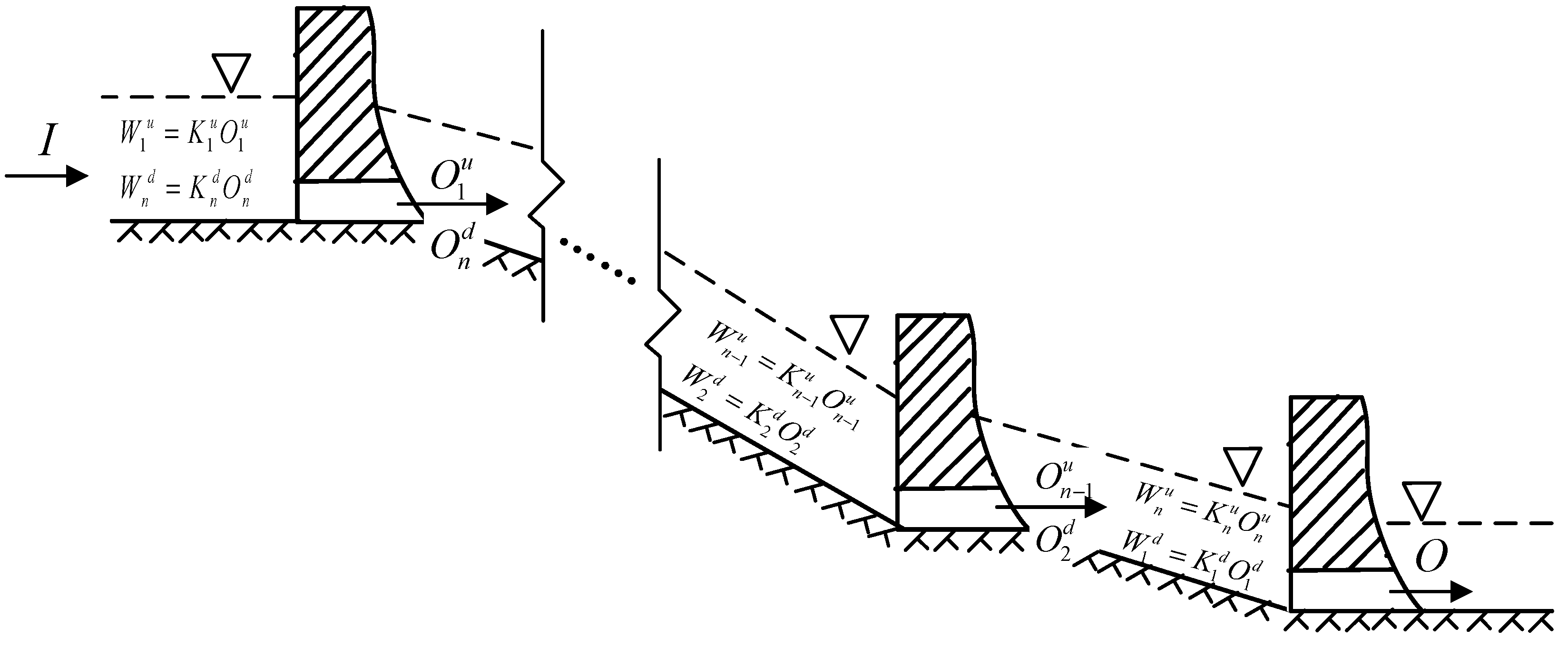
To account for the spatial heterogeneity in river flow routing, the river system is conceptualized as a cascade of unequal linear reservoirs, as shown in Figure 1. Structurally, it is similar to that of HIUH in Li et al. [26]. The main difference is that as a river flow routing approach, the heterogeneous DGNM (HDGNM) not only considers the contribution of the new water from upstream but also considers the contribution of the old water stored in river reach, which is a considerable component for river flow routing.

As illustrated in Figure 1, there are two numbering systems, named as “up-numbering system” and “down numbering system”, respectively. In the up-numbering system, reservoirs are numbered from upstream to downstream, denoted by superscript “u”. In the down-numbering system, reservoirs are numbered from downstream to upstream, denoted by superscript “d”. The outflow and storage of each reservoir are $O_i^u$ or $O_{n-i+1}^d$ and $W_i^u$ or $W_{n-i+1}^d$, respectively. The linear relationship between outflow and storage of each reservoir is given in Figure 1.

The conceptual interpretation of the DGNM shows that the downstream outflow is generated by the old water stored in the channel and the new water from upstream inflow, denoted by O^old and O^new, respectively, as

$$O_{t+1}^{old}={\displaystyle \sum _{j=0}^{n-1}{\displaystyle \sum _{i=0}^j\frac{{\left(-1\right)}^i}{j!}{C}_j^i\left(1-S_{n-j}^u\right)O_{t-i}}}$$

(5)

$$O_{t+1}^{new}=S_n^u{I}_t+\left(1-\frac{K}{\Delta t}{\displaystyle \sum _{i=1}^n{S}_i^u}\right)\Delta I_{t+1}$$

(6)

For the unequal linear cascade system, if the inflow I is a continuous unit inflow, then the outflow of each reservoir is $O_i^u=S_i^u$. The term $K_i{S}_i^u$, as interpreted in the DGNM, represents the water stored in each reservoir, and $1-{\sum }_{i=1}^n{K}_i{S}_i^u/\Delta t$ represents the ratio of water released from the channel during the period $\Delta t$. Then, $\left(1-{\sum }_{i=1}^n{K}_i{S}_i/\Delta t\right)\Delta I_{t+1}$ is the outflow generated by the inflow increment during the time interval $\left[t,t+\Delta t\right]$ after the channel routing. According to the conceptual interpretation of the DGNM, the outflow generated by the new water (upstream inflow) is composed by the responses of constant inflow $I_t$ and its increment, i.e.,

$$O_{t+1}^{new}=S_n^u{I}_t+\left(1-\frac{1}{\Delta t}{\displaystyle \sum _{i=1}^n{K}_i{S}_i^u}\right)\Delta I_{t+1}$$

(7)

The comparison between Equations (6) and (7) indicates that O^new can be obtained by replacing the storage parameter K and S-curve in Equation (6) with variable K_i and heterogeneous S-curve, respectively, in the unequal linear reservoir system. Not like O^new, K can be replaced by K_i directly. In the expression of O^old, K is not explicit in the equation, but implicit in the calculation of coefficients of S_n-j. Hence, O^old cannot be obtained by directly replacing K with K_i. For the sake of simplicity, down numbering system is used in deriving the calculation of O^old. In the down numbering system, the storage routing equation of the j-th reservoir can be obtained from the water balance equation:

$$K_j^d\frac{d{O}_j^d\left(t\right)}{dt}=O_{j+1}^d\left(t\right)-O_j^d\left(t\right)$$

(8)

Equation (8) demonstrates that the outflow of each reservoir at the current time is as follows:

$$O_1^d\left(t\right)=O\left(t\right)$$

$$O_2^d\left(t\right)=O\left(t\right)+K_1^d{O}^{\prime }\left(t\right)$$

$$O_3^d\left(t\right)=O\left(t\right)+\left(K_1^d+K_2^d\right)O^{\prime }\left(t\right)+K_1^d{K}_2^d{O}^{″}\left(t\right)$$

$$O_j^d\left(t\right)=O\left(t\right)+{\displaystyle \sum _{p=1}^{j-1}{\displaystyle \prod _{r_p>\cdots >r_1=1}^{j-1}\left(K_{r_1}^d\cdots K_{r_p}^d\right)O^{\left(p\right)}\left(t\right)}}$$

(9)

Based on the physical interpretation of the GNM [5], the recession flow of the current water storage in river channel is the superposition of the recession flow generated by the current water storage in each reservoir. According to the conception of linear reservoir, the current water storage of the j-th reservoir is $K_j^d{O}_j^d\left(t\right)$, which can be treated as an instantaneous inflow into each reservoir, then the outflow at the end of the period generated by each reservoir is $K_j^d{O}_j^d\left(t\right)u_j^d\left(\Delta t\right)$. Based on the principle of superposition, O^old is the outflow generated by the current water storage of all reservoirs, hence

$$\begin{gathered} {\mathrm{O}}_{t+1}^{old}={\displaystyle \sum _{j=1}^n{K}_j^d{O}_j^d\left(t\right)u_j^d\left(\Delta t\right)} \\ ={\displaystyle \sum _{j=1}^n{K}_j^d{u}_j^d}\left(\Delta t\right)\left[O\left(t\right)+{\displaystyle \sum _{p=1}^{j-1}{\displaystyle \prod _{r_p>\cdots >r_1=1}^{j-1}\left(K_{r_1}^d\cdots K_{r_p}^d\right)}}{O}^{\left(p\right)}\left(t\right)\right] \end{gathered}$$

(10)

The formula shows that the recession process can finally be expressed as a linear combination of 0~(n − 1) derivatives of the current time $O\left(t\right)$, which is

$$O_{t+1}^{old}={\displaystyle \sum _{p=0}^{n-1}{A}_p{O}_t^{\left(p\right)}}$$

(11)

where $A_p\left(p=0,\cdots ,n-1\right)$ is the coefficient of p-th order derivative of O(t), then we have (detailed derivation is provided in Appendix A)

$$A_p=\{\begin{array}{l}1-S_n^d,p=0\\ {\displaystyle \sum _{r_p>\cdots >r_1=1}^{n-1}\left(K_{r_1}^d\cdots K_{r_p}^d\right)\left(S_{r_p}^d-S_n^d\right),p>0}\end{array}$$

(12)

The calculation of A_p is a n-Choose-p combination problem. Define a set $A=\left(K_1^d,\cdots ,K_n^d\right)$, select p elements and multiply them by $\left(S_i^d-S_n^d\right)$ (i = p,…,n), respectively. Then, the summation of all these combinations is A_p. Though A_p is derived in the down numbering system, it still holds true for the up-numbering system because this combination problem is irrelevant to the numbering order. Hence, A_p can also be calculated by directly replacing the superscript “d” with “u” in the up-numbering system, ensuring that O^old and O^new are calculated under the same numbering system. To further discretize the term O^old in Equation (11), the derivatives of O(t) are approximated by the following backward finite difference method.

$$O_t^{\left(p\right)}=\frac{1}{\Delta t^p}{\displaystyle \sum _{i=0}^p{\left(-1\right)}^i{C}_p^i{O}_{t-i}}$$

(13)

Substituting Equations (12) and (13) into Equation (11), we obtain

$$O_{t+1}^{old}={\displaystyle \sum _{p=0}^{n-1}{\displaystyle \sum _{i=0}^p\frac{{\left(-1\right)}^i}{\Delta t^p}{C}_p^i{A}_p{O}_{t-i}}}$$

(14)

Combined with the conceptual interpretation of the DGNM, we have

$$O_{t+1}={\displaystyle \sum _{j=0}^{n-1}{\displaystyle \sum _{i=0}^j\frac{{(-1)}^i}{\Delta t^j}{C}_j^i{A}_j^{}{O}_{t-i}}}+S_n{I}_t+\left(1-\frac{1}{\Delta t}{\displaystyle \sum _{i=1}^n{K}_i{S}_i}\right)\Delta I_{t+1}$$

(15)

Equation (15) is the calculation formula of HDGNM, and it is also the discrete solution of linear cascade model with unequal reservoirs under nonzero initial conditions. Combined conceptual interpretation of the DGNM into mathematical derivation, the HIUH or heterogeneous S-curve with a consideration of the spatial heterogeneity in the storage routing, was successfully incorporated in the DGNM. Hence, the HDGNM is applicable to the river reach with large changes of cross-sections and slopes.

2.4. Parameter Estimation Method

Parameter n and K_i in HDGNM can be obtained in two different ways, one is optimized by intelligent algorithm, another is estimated on the basis of the reliable relationships between model parameters and physical characteristics.

The SCE-UA algorithm is a successfully proven method in global optimization that was originally developed at the University of Arizona [27] and was extensively used in hydrological model calibration over the past several decades. This algorithm combines complex procedures with the concepts of competition evolution, complex shuffling, and controlled random search to acquire a global optimal estimation. The main calculation steps of SCE-UA algorithm can be seen in Duan et al. [27]. Comparisons with other algorithms such as the Genetic Algorithms (GA) and Simulated Annealing (SA) suggest the SCE-UA could obtain a more robust and reliable solution especially in terms of identification and calibration problems [28]. This algorithm is thus used to optimize the model parameters. Moreover, the root mean square error (RMSE) is a measure regularly used in model performance evaluations [29], thus we selected it as the objective function.

Besides, both parameters n and K_i in HDGNM have clear physical interpretations, thus possible to determine the model parameters under insufficient observed data. Parameter n is the number of linear reservoirs or subreaches for simplicity. The storage coefficient K_i has a physical meaning of travel time through a subreach, which can be estimated as follows [30].

$$K_i=\frac{L_i}{c_i}$$

(16)

where L_i is the reach length, and c_i is the celerity, which can be calculated by

$$c_i=m{v}_i$$

(17)

where v_i is the average velocity, and m is a factor relating average velocity and celerity.

The value of m is 5/3 when applying Manning’s flow resistance formula to a rectangular channel cross section. For a channel with a wide-shallow section as in a river, the average velocity can be calculated approximately by the Manning equation [31]

$$v_i=\frac{1}{n_M}{h}_i^{\frac{2}{3}}{J}_i^{\frac{1}{2}}$$

(18)

where $n_M$ is the roughness coefficient, h is the average depth, and J is the bed slope.

3. Application

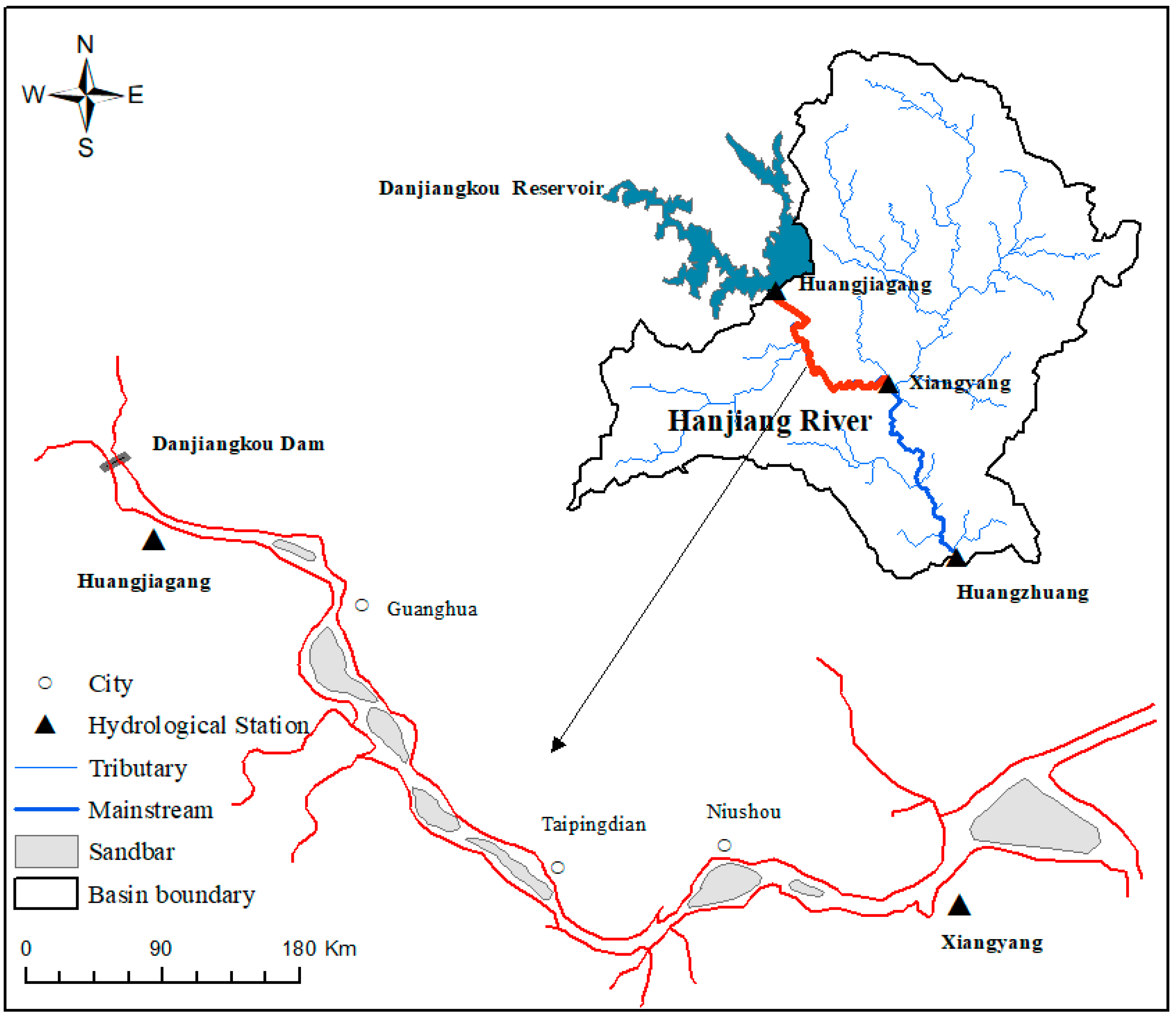
To test the applicability of the HDGNM, the river reach between gauging stations Huangjiagang and Xiangyang in the Hanjiang River of China is selected as a case study. Hanjiang River is one of the most important tributaries of the Yangtze River of China. The Danjiangkou reservoir, located on the upper Hanjiang River, is the water source of the middle route of China’s south-to-north water transfer project. Since the opening of the first phase of the middle route on 12 December 2014, the Danjiangkou reservoir has supplied more than 40 billion cubic meters of water to drier north areas in China, thereby benefiting 79 million people in Beijing, Tianjin, Hebei province, and Henan province. The studied river reach with a length of 105 km is located in the middle Hanjiang River, where the Huangjiagang hydrological station is located at 6 kms downstream of the Danjiangkou dam site and serves as the outflow control station of the Danjiangkou reservoir. The interval basin area between Huangjiagang and Xiangyang is 8044 km². The sketch map of the middle-Hanjiang River and the studied river reach are shown in Figure 2. The studied river reach is located in the hilly and plain areas, where hills, terraces, artificial narrows, and wide valleys distribute alternatively, and showing obvious lotus root node shape on the plane. The main channels in wide sections have large swings and many beaches, but become single in narrow sections, which makes a large change of the shape in the sections along the river reach, as shown in Figure 2. Based on the location of cities, the river reach can be divided into four sub-reaches [32], namely, Huangjiagang-Guanghua (H-G), Guanghua-Taipingdian (G-T), Taipingdian-Niushou (T-N), and Niushou-Xiangyang (N-X). The mean slopes of these four sub-reaches are 1.76 × 10⁻⁴, 2.76 × 10⁻⁴, 2.21 × 10⁻⁴, and 2.14 × 10⁻⁴, respectively. The channel slope of the studied river reach changes largely, especially from subreach H-G to subreach G-T. In short, the topography of the studied river reach varies greatly.

The runoff data in flood season of the Huangjiagang and Xiangyang hydrological stations from the year 1974 to 2011 were collected from the Bureau of Hydrology, Changjiang Water Resources Commission in China. Almost all hydrologic routing methods are based on the water balance equation of the river reach. A large lateral inflow would break this balance and influence the accuracy, so low proportion (less than 10% in this study) of the lateral inflows is required in selecting flood events, and the difference between the total outflow and total inflow for each event is proportionately distributed to the upstream inflow. Ten flood events fulfilling these criteria were selected to test the proposed model. The time step of the HDGNM is fixed to 3 h, thus the flood records were interpolated into a time interval of 3 h.

The selected 10 flood events were further partitioned into calibration data and validation data. The calibration data was used to calibrate the model parameters. The validation data were used to assess the out-of-sample performance. We used 8 flood events observed during the year 1975 to 2005 for calibration and the other 2 flood events happened in 2007 and 2011 for validation.

The goodness-of-fit between the computed and observed hydrographs was quantitatively and less subjectively tested using the model evaluation metrics. These metrics were used to measure the deviations of different hydrograph components, such as the peak flow rate and hydrograph. Percentage errors in computed and observed peak flow rates were usually determined using the relative error of peak discharge (E_P) which is defined as follows [33]:

$$E_P=\frac{\left|O_{p,est}^{}-O_{p.obs}^{}\right|}{O_{p.obs}^{}}\times 100\%$$

(19)

where O_p,est and O_p,obs are the estimated and observed peak discharge, respectively.

The E_P statistic was used to assess the model performance in peak flow rates, ignoring the shape of the computed and observed hydrographs. To overcome this, Nash and Sutcliffe [34] proposed a dimensionless coefficient of model efficiency (E_NS), given as:

$$E_{NS}^{}=1-\frac{{\displaystyle \sum _{t=1}^T{(O_{t,est}^{}-O_{t,obs}^{})}^2}}{{\displaystyle \sum _{t=1}^T{(O_{t,obs}^{}-{\overline{O}}_t^{})}^2}}$$

(20)

where O_t,est and O_t,obs are estimated and observed discharge at time t, respectively. ${\overline{O}}_t^{}$ represents the mean of observed discharge. The E_NS statistic provides a well-accepted measure of fit between computed and observed hydrographs, its value increasing toward unity as the fit of the simulated hydrograph progressively improves.

Moreover, Percent bias (PBIAS) is usually used in combination with Nash-Sutcliffe efficiency to evaluate the robustness of simulated data. It quantified the deviations between the simulated data and the observed data; low-magnitude values indicate an accurate model simulation, and 0.0 is the optimal value. A positive value indicates that the model underestimates the bias, while a negative value indicates that the model overestimates the bias [35]. It can be calculated as follows:

$$PBIAS=\frac{{\displaystyle \sum _{t=1}^T(O_{t,obs}^{}-O_{t,est}^{})}}{{\displaystyle \sum _{t=1}^T{(O_{t,obs}^{})}^{}}}\times 100\%$$

(21)

where $PBIAS$ is the bias of the evaluated data, expressed as a percentage.

4. Results and Discussion

The comparison between the DGNM and other models, including the widely used Muskingum method and dynamic wave model (DWM), was made in Yan et al. [20]. The results show that the DGNM can provide comparable (to DWM) or even better results (to Muskingum), thus the DGNM was selected as a performance benchmark. The SCE-UA algorithm was employed to obtain the parameters of these two models, and the results of the optimization were that n = 3, K = 3.51 h for the DGNM and n = 3, K₁ = 1.58 h, K₂ = 8.80 h, K₃ = 1.59 h for the HDGNM. The numbers of the linear reservoirs are both expected to be three in these two models. The difference lies in the storage parameter K. In the DGNM, the three linear reservoirs are equivalent, which is essentially a homogenization of the topographical differences of the subreaches. However, in the HDGNM, two of the three linear reservoirs with K₁ = 1.58 h and K₃ = 1.59 h are approximately the same, and the other one is quite different from the two with a value of 8.80 h. Therefore, the HDGNM can more objectively reflect the influence of topographical differences on the storage routing of the river channel, and thus can improve the accuracy of the flood routing.

To further test the validity of the parameter calculation from calibration, the verification experiment has also been carried out. The other 2 observed flood events in the year 2007 and 2011 were adopted to verify the calibration results. The accuracy evaluation results of these two models in calibration and validation periods were both shown in

Table 1. Accuracy evaluation results of DGNM and HDGNM.

Period	Date	DGNM			HDGNM (Optimized)			HDGNM (Estimated)
		EP (%)	ENS	PBIAS (%)	EP (%)	ENS	PBIAS (%)	EP (%)	ENS	PBIAS (%)
Calibration	Oct-1974	0.91	0.9930	0.30	4.27	0.9861	1.05	2.60	0.9905	−0.09
	Sep-1975	3.69	0.9918	−0.91	2.87	0.9950	−0.03	3.01	0.9812	−0.92
	Jul-1980	1.62	0.9043	−2.20	1.08	0.9284	−1.67	0.20	0.8406	−1.62
	Aug-1981	5.26	0.9699	−0.77	3.47	0.9747	−0.38	6.14	0.9632	−0.44
	Sep-1981	7.82	0.9655	−1.77	4.45	0.9806	−1.02	9.43	0.9363	−0.56
	Sep-1984	0.99	0.9774	−2.15	1.78	0.9860	−1.52	2.29	0.9576	−1.31
	Sep-2003	2.54	0.9655	1.45	0.77	0.9715	1.44	2.03	0.9476	1.69
	Oct-2005	8.72	0.9845	0.14	0.63	0.9963	0.26	12.20	0.9666	0.51
	Average	3.94	0.9690	−0.74	2.42	0.9773	−0.23	4.74	0.9480	−0.34
Validation	Jul-2007	0.62	0.9707	0.05	0.66	0.9775	0.06	5.11	0.9471	0.05
	Sep-2011	2.48	0.9889	−1.53	0.32	0.9928	−1.42	2.32	0.9825	−1.31
	Average	1.55	0.9798	−0.74	0.49	0.9852	−0.68	3.72	0.9648	−0.63

.

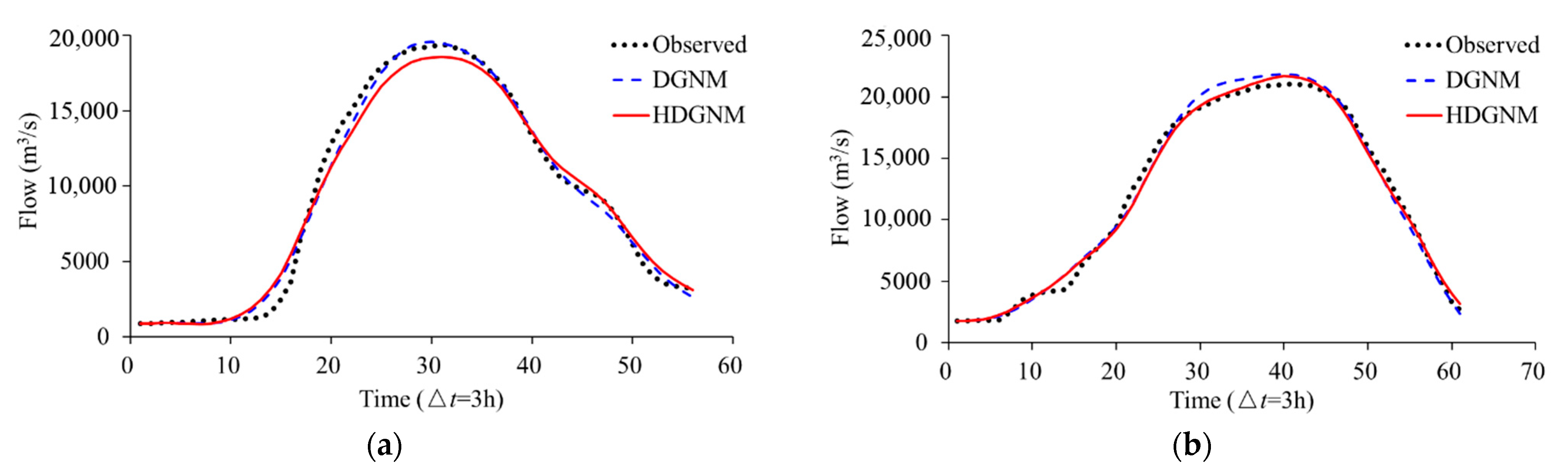
In calibration period, the average values of E_P, E_NS, and PBIAS were 3.94%, 0.9690, and −0.74% for DGNM, respectively. Compared with that of the DGNM, the HDGNM with optimized parameters made some improvements; the average value of E_P reduced to 2.42%, that of E_NS increased to 0.9773, and the average magnitude value of PBIAS was also reduced to −0.23%. The similar improvements can be found in the validation period with values from 1.55–0.49% for E_P, from 0.9798–0.9852 for E_NS, and from −0.74 to −0.68% for PBIAS, respectively. Except for the October 1974 flood event, the other 9 flood events were improved in different levels. Visual comparisons of the computed and observed hydrographs can provide a quick and simple means of assessing the performance of the proposed model, as shown in Figure 3. The HDGNM with a consideration of the topographical heterogeneity of the river reach, makes the computed hydrographs much closer to the measured hydrographs, especially near the flood peaks. The adaptability of the DGNM was increased when the spatial heterogeneity is accounted for, and thus the HDGNM is more applicable, especially in the river reaches where the river slopes and cross-sections change greatly.

In the above comparison, parameters were optimized by intelligent algorithm, which usually achieves the best accuracy. However, the optimization technique is more applicable to flood routing in gauged basins due to its requirement of large amounts of observed data [36]. In case where any measurements are not available, sufficiently long streamflow time series for parameter calibration is typically not available, leading to difficulties to predict flow characteristics [37]. One common way to deal with this problem is the regionalization of model parameters according to the physical characteristics of basins [38]. The interpretation of HDGNM parameters in terms of the physical characteristics extends the applicability of the model to ungauged basins. Both parameters n and K_i in HDGNM have clear physical interpretations, and thus can be estimated in terms of the physical characteristics including reach length, average depth, and bed slope, as shown in Equations (18–20). The reach lengths and bed slopes of four sub-reaches in this study were found in Gong [32]. Manning’s roughness coefficient of the middle-lower Hanjiang river was suggested to have values of 0.027–0.030 by Wang et al. [39]. In this study, the Manning’s roughness coefficient is set to 0.028 in each sub-reach for simplicty. Due to a lack of data about the bottom elevation along the river reach, the average depths are calculated instead by the difference between the maximum and minimum water levels. According to the observed data, the average depths at Huangjiagang and Xiangyang sections are 7.54 m and 7.49 m, respectively. We set that h = 7.50 m for each subreach finally. The details of physical characteristics as well as the parameter K_i of subreaches are listed in

Table 2. Physical characteristics of river reaches in middle-Hanjiang River.

Parameter	Interpretation	Sub-Reaches
		H-G	G-T	T-N	N-X
L	Reach Length (km)	25.59	37.63	24.00	19.13
${\mathrm{n}}_{\mathrm{M}}$	Roughness Coefficient	0.028	0.028	0.028	0.028
J	Bed Slope (10−4)	1.76	2.76	2.21	2.14
h	Average Depth (m)	7.50	7.50	7.50	7.50
K	Storage Parameter (h)	2.33	2.74	1.95	1.58

. Based on the estimated parameters, the outflow of the selected floods was calculated by Equation (15). The accuracy evaluation results were shown in Table 1 referred as HDGNM (estimated). The average values of E_P, E_N and PBIAS were 4.74%, 0.9480, and −0.34% in calibration period, and 3.72%, 0.9648, and −0.63% in validation period, respectively, meaning the estimation method is acceptable.

On the other hand, traditional routing models, such as the Muskingum model and DGNM, estimate the parameters using the basin characteristics representing the inlet and outlet of the river reach [40], therefore the simulation is limited to the outflow. By adjusting the parameter n, the HDGNM with variable parameters can estimate flood process of any section between the inlet and outlet. From this perspective, most traditional routing models are lumped whereas the HDGNM is semidistributed. Figure 4 shows an example calculated by the flood event in Oct-1974. When n is set to 1, 2, 3, and 4 in Equation (15), respectively, the flood hydrograph of each section from upstream to downstream can be easily obtained. The sections from upstream to downstream are Guanghua, Taipingdian, and Niushou in turn, and Xiangyang is the outlet section. Only the observed outflow at the outlet section was shown due to a lack of the observed data for other sections in Figure 4. In a nutshell, the HDGNM using the SCE-UA algorithm can achieve the best simulation results in gauged basins, while the estimation method based on the physical characteristics makes the HDGNM transfer well to the ungauged basins. What’s more, as a semidistributed model, the HDGNM has a potential to estimate the flood process of any section between the inlet and outlet.

5. Conclusions

This paper proposed a conceptual hydrologic flood routing approach—HDGNM, which takes into account the spatial heterogeneity in the modelling by incorporating the HIUH or S-curve into the DGNM. The spatial heterogeneity of a river reach is reflected by a series of unequal linear reservoirs. It is hard work to deduce the HDGNM under unequal linear cascade system directly. The conceptual interpretation of the components of the DGNM was employed in the process of derivation. The discharge produced by the upstream inflows was deduced by directly replacing the S-curve with heterogeneous S-curve, and the recession produced by the channel storage was obtained by the superposition of the recession process of each linear reservoir, which was calculated by the impulse response of the stored water with the help of HIUH. The outflow in the HDGNM was composed of these two parts conceptually and was formally expressed as a weight of the inflows and outflows, whose weight coefficients were calculated by the heterogeneous S-curve.

The proposed HDGNM was evaluated on a reach of the Hanjiang River in China from Huangjiagang down to Xiangyang. The slopes and cross-sections of this reach changes largely, and thus the capacity of the storage routing in each subreach is different too. Three equivalent linear reservoirs were conceptualized in the DGNM, but a significantly different linear reservoir with a much larger storage coefficient was detected from the other two reservoirs in the HDGNM. Such difference partially reflected the spatial heterogeneity of the river reach, making the HDGNM more adaptive than the DGNM. The simulation results suggest that addressing the spatial heterogeneity, the HDGNM outperforms the DGNM in terms of model efficiency and relative error. From a physical point of view, the storage coefficient K is a reservoir detention characteristic and has a physical meaning of travel time. Physically, the changes in slope and cross-sections are expected to influence travel times and distortion of the flood wave. This influence can then be reflected by the storage coefficient K. In the DGNM, all linear reservoirs have the same K, the abrupt changes of the slope and cross-sections cannot be addressed. In contrast, with different K, the HDGNM is more adaptive to these changes. Furthermore, the parameters have specific physical meanings, extending the applicability of the model to ungauged basins. By adjusting the parameter n, the HDGNM can be developed as a semidistributed model. These outcomes indicate that the model is applicable even for ungauged case studies.

References

- Arora, V.; Seglenieks, F.; Kouwen, N.; Soulis, E. Scaling aspects of river flow routing. Hydrol. Process. 2001, 15, 461–477. [Google Scholar] [CrossRef]
- Weinmann, P.E.; Laurenson, E.M. Approximate Flood Routing Methods: A Review. J. Hydraul. Div. 1979, 105, 1521–1536. [Google Scholar] [CrossRef]
- Singh, V.P.; Wang, G.-T.; Adrian, D.D. Flood routing based on diffusion wave equation using mixing cell method. Hydrol. Process. 1997, 11, 1881–1894. [Google Scholar] [CrossRef]
- McCarthy, G.T. The unit hydrograph and flood routing. In Conference of North Atlantic Division; US Army Corps of Engineers, US Engineering Office: Providence, RI, USA, 1938. [Google Scholar]
- Yan, B.; Guo, S.; Liang, J.; Sun, H. The generalized Nash model for river flow routing. J. Hydrol. 2015, 530, 79–86. [Google Scholar] [CrossRef]
- Shaw, E.M. Hydrology in Practice; TJ Press (Padstow) LTD: Cornwall, UK, 1994. [Google Scholar]
- Cunge, J.A. On the subject of a flood propagation computation method (Muskingum method). J. Hydrol. Res. 1969, 7, 205–230. [Google Scholar] [CrossRef]
- Norouzi, H.; Bazargan, J. Flood routing by linear Muskingum method using two basic floods data using particle swarm optimization (PSO) algorithm. Water Supply 2020, 20, 1897–1908. [Google Scholar] [CrossRef]
- Badfar, M.; Barati, R.; Dogan, E.; Tayfur, G. Reverse Flood Routing in Rivers Using Linear and Nonlinear Muskingum Models. J. Hydrol. Eng. 2021, 26, 04021018. [Google Scholar] [CrossRef]
- Moramarco, T.; Fan, Y.; Bras, R.L. Analytical Solution for Channel Routing with Uniform Lateral Inflow. J. Hydraul. Eng. 1999, 125, 707–713. [Google Scholar] [CrossRef]
- Todini, E. A mass conservative and water storage consistent variable parameter Muskingum-Cunge approach. Hydrol. Earth Syst. Sci. 2007, 4, 1645–1659. [Google Scholar] [CrossRef] [Green Version]
- Nash, J.E. The form of the instantaneous unit hydrograph. IAHS Publ. 1957, 45, 114–121. [Google Scholar]
- Kalinin, G.; Milyukov, P. On the computation of unsteady flow in open channels. Met. Gidrol. 1957, 10, 10–18. [Google Scholar]
- Chow, V.T.; Maidment, D.R.; Mays, L.W. Applied Hydrology; McGraw-Hill: New York, NY, USA, 1988. [Google Scholar]
- Szöllösi-Nagy, A. The discretization of the continuous linear cascade by means of state space analysis. J. Hydrol. 1982, 58, 223–236. [Google Scholar] [CrossRef]
- Szollosi-Nagy, A. Input detection by the discrete linear cascade model. J. Hydrol. 1987, 89, 353–370. [Google Scholar] [CrossRef]
- Szilagyi, J. State-space discretization of the KMN-cascade in a sample-data system framework for streamflow forecasting. J. Hydrol. Eng. 2003, 8, 339–347. [Google Scholar] [CrossRef] [Green Version]
- Szilagyi, J. Discrete state-space approximation of the continuous Kalinin–Milyukov–Nash cascade of noninteger storage elements. J. Hydrol. 2006, 328, 132–140. [Google Scholar] [CrossRef] [Green Version]
- Szilagyi, J.; Laurinyecz, P. Accounting for Backwater Effects in Flow Routing by the Discrete Linear Cascade Model. J. Hydrol. Eng. 2014, 19, 69–77. [Google Scholar] [CrossRef] [Green Version]
- Yan, B.; Huo, L.; Liang, J.; Yang, W.; Zhang, J. Discretization of the Generalized Nash Model for Flood Routing. J. Hydrol. Eng. 2019, 24, 04019029. [Google Scholar] [CrossRef]
- Rodríguez-Iturbe, I.; Valdés, J.B. The geomorphologic structure of hydrologic response. Water Resour. Res. 1979, 15, 1409–1420. [Google Scholar] [CrossRef] [Green Version]
- Rinaldo, A.; Rodriguez-Iturbe, I. Geomorphological Theory of the Hydrological Response. Hydrol. Process. 1996, 10, 803–829. [Google Scholar] [CrossRef]
- Hayami, S. On the propagation of Flood Waves. Disaster Prev. Res. Inst. Bull. 1951, 1, 1–16. [Google Scholar]
- Moussa, R.; Bocquillon, C. Criteria for the choice of flood routing methods in natural channels. J. Hydrol. 1996, 186, 1–30. [Google Scholar] [CrossRef]
- Adhikary, P.P.; Sena, D.R.; Dash, C.J.; Mandal, U.; Nanda, S.; Madhu, M.; Sahoo, D.C.; Mishra, P.K. Effect of Calibration and Validation Decisions on Streamflow Modeling for a Heterogeneous and Low Runoff–Producing River Basin in India. J. Hydrol. Eng. 2019, 24, 05019015. [Google Scholar] [CrossRef]
- Li, C.; Guo, S.; Zhang, W.; Zhang, J. Use of Nash’s IUH and DEMs to identify the parameters of an unequal-reservoir cascade IUH model. Hydrol. Process. 2008, 22, 4073–4082. [Google Scholar] [CrossRef]
- Duan, Q.; Sorooshian, S.; Gupta, V.K. Optimal use of the SCE-UA global optimization method for calibrating watershed models. J. Hydrol. 1994, 158, 265–284. [Google Scholar] [CrossRef]
- Naeini, M.R.; Analui, B.; Gupta, H.V.; Duan, Q.; Sorooshian, S. Three decades of the Shuffled Complex Evolution (SCE-UA) optimization algorithm: Review and applications. Sci. Iran. 2019, 26, 2015–2031. [Google Scholar]
- Chai, T.; Draxler, R.R. Root mean square error (RMSE) or mean absolute error (MAE)?—Arguments against avoiding RMSE in the literature. Geosci. Model Dev. 2014, 7, 1247–1250. [Google Scholar] [CrossRef] [Green Version]
- Perumal, M. Multilinear muskingum flood routing method. J. Hydrol. 1992, 133, 259–272. [Google Scholar] [CrossRef]
- Perumal, M.; Moramarco, T.; Sahoo, B. A methodology for discharge estimation and rating curve development at ungauged river sites. Water Resour. Res. 2007, 43, W02412. [Google Scholar] [CrossRef]
- Gong, G. Channel changes in the Hanjiang River below the Danjiangkou reservoir. Georg. Res. 1982, 1, 69–78. [Google Scholar]
- Green, I.R.A.; Stephenson, D. Criteria for comparison of single event models. Hydrol. Sci. J. 1986, 31, 395–411. [Google Scholar] [CrossRef] [Green Version]
- Nash, J.E.; Sutcliffe, J.V. River flow forecasting through conceptual models part I—A discussion of principles. J. Hydrol. 1970, 10, 282–290. [Google Scholar] [CrossRef]
- Moriasi, D.N.; Arnold, J.G.; Van Liew, M.W.; Bingner, R.L.; Harmel, R.D.; Veith, T.L. Model Evaluation Guidelines for Systematic Quantification of Accuracy in Watershed Simulations. Trans. ASABE 2007, 50, 885–900. [Google Scholar] [CrossRef]
- Song, X.M.; Kong, F.Z.; Zhu, Z.X. Application of muskingum routing method with variable parameters in ungauged basin. Water Sci. Eng. 2011, 20, 1–12. [Google Scholar]
- Sivapalan, M.; Takeuchi, K.; Franks, S.; Gupta, V.K.; Karambiri, H.; Lakshmi, V.; Liang, X.; Mcdonnell, J.; Mendiondo, E.M.; O’Connell, P.E.; et al. IAHS Decade on Predictions in Ungauged Basins (PUB), 2003–2012: Shaping an exciting future for the hydrological sciences. Hydrol. Sci. J. 2003, 48, 857–880. [Google Scholar] [CrossRef] [Green Version]
- Yadav, M.; Wagener, T.; Gupta, H. Regionalization of constraints on expected watershed response behavior for improved predictions in ungauged basins. Adv. Water Resour. 2007, 30, 1756–1774. [Google Scholar] [CrossRef]
- Wang, Y.; Zhang, W.; Zhao, Y.; Peng, H.; Shi, Y. Modelling water quality and quantity with the influence of inter-basin water diversion projects and cascade reservoirs in the Middle-lower Hanjiang River. J. Hydrol. 2016, 541, 1348–1362. [Google Scholar] [CrossRef]
- Yoo, C.; Lee, J.; Lee, M. Parameter Estimation of the Muskingum Channel Flood-Routing Model in Ungauged Channel Reaches. J. Hydrol. Eng. 2017, 22, 05017005. [Google Scholar] [CrossRef]
Figure 1.
Schematic of HDGNM.
Figure 2.
Sketch map of middle-Hanjiang River and studied river reach.
Figure 3.
Comparison of computed and observed hydrographs for selected 10 floods. (a) Oct-1974, (b) Sep-1975, (c) Jul-1980, (d) Aug-1981, (e) Sep-1981, (f) Sep-1984, (g) Sep-2003, (h) Oct-2005, (i) Jul-2007, and (j) Sep-2011.
Figure 4.
Flood hydrographs of sections between Huangjiagang and Xiangyang.