Hydrodynamic Evaluation of Five Influent Distribution Systems in a Cylindrical UASB Reactor Using CFD Simulations

Abstract

UASB reactors are a promising option for environmentally friendly wastewater treatment due to their reduced carbon footprint and their capacity to treat a variety of wastewater strengths, among other recognized advantages over alternative wastewater treatment systems. The Influent Distribution System (IDS) is a critical structure for generating granules in a UASB reactor since it provides the required flow hydrodynamics for their formation. Thus, the objective of this study was to evaluate and compare the efficiency of five IDS configurations to generate ideal granulation conditions using Computational Fluid Dynamics (CFD) simulations. The IDS configurations were as follows: (C1) single radial inflow, (C2) upward axial inflow, (C3) downward distributed axial inflow, and two novel configurations in the form of (C4) double opposite radial inflow and (C5) downward tangential inflow. The hydrodynamic response of configuration C1 was validated in a physical model with dynamic Froude similitude. The granulation measurement was velocity-based in the reactor reaction zone using steady-state CFD simulations. The novel IDS configuration C4 was the one that resulted in the highest granulation volume, with up to 45.5% of the potential granulation volume of the UASB reactor, in contrast to the IDS C2 that obtained the lowest granulation with only 10.8%. Results confirm that the IDS directly impacts the hydrodynamics of the reactor and that model-based design can be used to ascertain IDS configurations that better promote granulation in UASB reactors.

1. Introduction

Anaerobic biological wastewater treatment technologies generate high expectations in the field of environmental sanitation because, in addition to having the ability to treat a variety of wastewater strengths [1,2,3], they are more environmentally sustainable technologies than their aerobic counterparts [4]. Anaerobic technologies could replace or complement aerobic-based treatment systems due to the advantages they provide, including biogas recovery, low excess sludge production, low construction, and operating costs, as well as low footprint and nutrient requirements [5]. Thus, anaerobic technologies will be crucial to comply with goals 6 and 7 of the United Nations 2030 Sustainable Development Agenda [6].

The Upflow Anaerobic Sludge Blanket (UASB) reactor is one of the most remarkable high-rate anaerobic wastewater treatment technologies. The UASB, developed by Lettinga et al. [7], is recognized as the most commonly used anaerobic wastewater treatment system on the planet [8], especially in South America and South Asia [9]. The generation of granular sludge is one of the main factors that has influenced the success of the UASB reactor since its presence allows treating wastewater with high organic loads in small volume reactors [10]. The microbial aggregate (i.e., granules) constituents of the granular sludge are formed by a multispecies bacterial consortium (hydrolytic, fermentative, acetogenic, and methanogenic bacteria) in a syntrophic relationship, which form inside the reactor during its start-up stage [11]. Microorganisms tend to develop into granules as a form of protection against predators and unfavorable environmental conditions [12]. Unlike flocculant sludge, granular sludge is dense and compact, which benefits its settling properties [13]. Furthermore, the limited diffusion within the granules makes them more resistant to the presence of toxins and to process shocks [14].

Although the driving forces for the development of granules are not well understood, it is known that environmental factors (e.g., temperature, pH), chemical factors (e.g., polymers and cations), and operational factors (e.g., reactor hydrodynamic conditions, substrate, and seed characteristics) play an essential role in their development [15,16]. According to Noyola and Moreno [17], within a UASB reactor, the most critical factor for the formation of granules is the upward flow velocity, confirming the hypothesis of the selection pressure theory of Hulshoff Pol et al. [18]. This theory suggests that during the reactor start-up stage if no inoculum has been added, dispersed microbial congregations (i.e., flocs) form [11]. The selection pressure takes effect when the upward velocities wash the light and disperse sludge out, retaining only the heaviest particles within the reactor, which become organic or inorganic nuclei for granule formation. The granules increase in size up to a certain limit until part of their structure collapses, generating new growth nuclei [19]. Under conditions of low selection pressure, biomass growth occurs mainly as flocculant sludge, a low-density suspended sludge with unfavorable settling properties [20], that is easily expelled from the reactor, deteriorating the quality of the effluent.

The Influent Distribution System (IDS) is a key structure in the UASB reactor. It is responsible for properly distributing the water inflow, substrate, and nutrients so that the granulation process occurs properly [21]. The IDS is directly related to the hydrodynamics of the reactor and, therefore, to the selective pressure that it can exert on the granule growth nuclei. In addition, its configuration can favor or disfavor the formation of channeling and stagnant zones, reducing the effective volume of the reactor, increasing the required time to obtain a viable granular sludge inventory (i.e., start-up time). UASB design guidelines recommend that the IDS be composed of multiple pipes discharging the inflow to the bottom of the reactor. This configuration attempts to distribute the flow evenly, which would result in homogeneous upward flow velocities [10,22,23,24]. However, many research works underestimate the influence of IDS on the reactor start-up time and its overall efficiency. Research on UASB reactors by Yang, Wang, et al. [25], Ozgun, Ersahin, et al. [26], or Singh and Viraraghavan [27], just to mention a few cases, use IDS configurations that are far from the recommended conditions, which would affect the hydrodynamics of the reactor. Without incorporating appropriate hydrodynamic characterizations, the usefulness of the results in UASB reactor studies may be limited, as they are difficult to evaluate, compare, and apply in practice. The flow hydrodynamics of the reactor can be influenced by the reactor configuration (e.g., IDS or gas-liquid-solid separator), by the operating conditions (e.g., flow rate, flow regime), or even by environmental conditions (e.g., temperature, wind).

For this reason, special care must be taken when designing full-scale UASB reactors using extrapolated results from studies that used reactors with different hydrodynamic characteristics. This fact even applies to design guidelines, whose recommendations are based on operational experience and hydrodynamic conditions that are unlikely to be accurately met when implementing new systems. The extrapolation of data can lead to the construction of reactors with treatment efficiencies that differ from those expected, resulting in economic losses. Therefore, to conclude a full-scale reactor design, its hydrodynamic characteristics must be verified either in a pilot-scale reactor or in a laboratory-scale reactor under dynamic similitude [28,29]. However, creating and monitoring physical models is costly, time-consuming, and typically only a limited number of configurations and operational scenarios can be assessed. These limitations can be overcome by using computational fluid dynamics (CFD), which allows the simulation of reactor flow behavior under various geometric, environmental, and operating conditions. Although a validation stage is required for a CFD simulation using data from physical models, this approach significantly reduces design costs. Thus, using CFD model-based design is increasingly common in wastewater treatment [30,31,32,33,34].

CFDs have been applied in UASB reactors, especially for reactor design and hydrodynamic evaluation. Souza et al. [35] hydrodynamically characterized the settling zone in a UASB reactor using CFDs. The authors found that the recirculation patterns produced by the GLSS significantly contributed to the separation of solids from the treated flow. Similarly, Wongnoi et al. [36] modified a GLSS using a model-based design approach, obtaining a more efficient structure that reduced the premature exit of solids from the reactor. Other studies using the technique have revealed, for instance, the presence of a discontinuity in the flow within the reaction zone [37] or that the water inlet velocity directly relates to the height of the sludge layer [38]. However, there is an information gap on the relationship between IDS configurations and their potential for granule production. CFD tools can be used to determine the IDS configuration that offers the greatest benefits for developing granular sludge and reducing the start-up time in UASB reactors. Although the start-up of a reactor can be accelerated by incorporating a granular seeding from another system, its acquisition and transport are expensive, and its availability is usually limited [16]. In addition, this approach requires long periods and special care of the granules to adapt to the new operating and treatment conditions. Therefore, the best option continues to be the generation of granular sludge directly with the wastewater and under the reactor’s actual operating conditions. Finding an IDS configuration that provides the highest granulation rate at the lowest implementation, operation, and maintenance costs is a critical requirement for advancing the development of UASB reactors. This advance would better promote the expansion of this type of reactor, significantly reducing the environmental impact generated by conventional wastewater treatment systems.

This study aims to characterize and compare the flow hydrodynamics and granulation conditions produced by five IDS configurations in a cylindrical UASB reactor in its start-up stage using 3D single-phase CFD simulations. The selected IDS configurations are those commonly reported in the literature and design guidelines, i.e., single radial inflow (C1), upward axial inflow (C2), and downward distributed axial inflow (C3). The two additional configurations are opposite double radial inflow (C4) and downward tangential inflow (C5), which are novel design-based IDS configurations proposed by the authors and included herein to ascertain if they could improve the hydraulic efficiency of the reactor by increasing the granulation volume in the reaction zone.

2. Materials and Methods

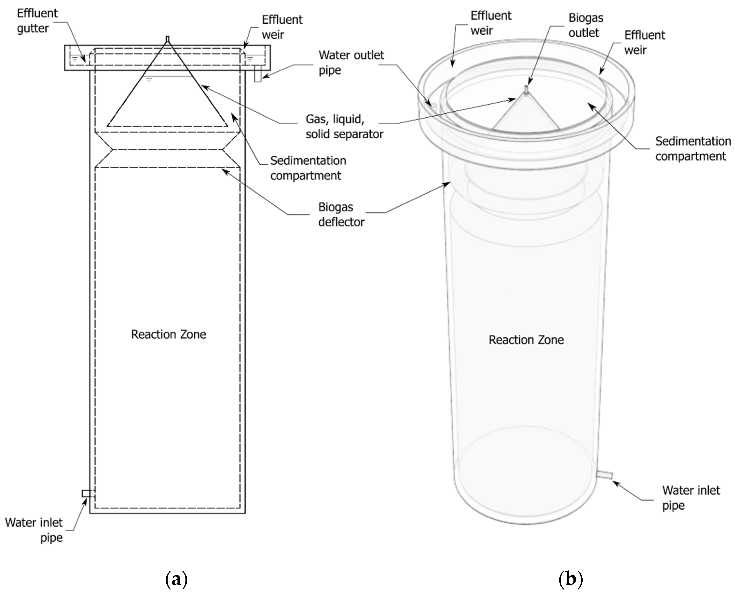
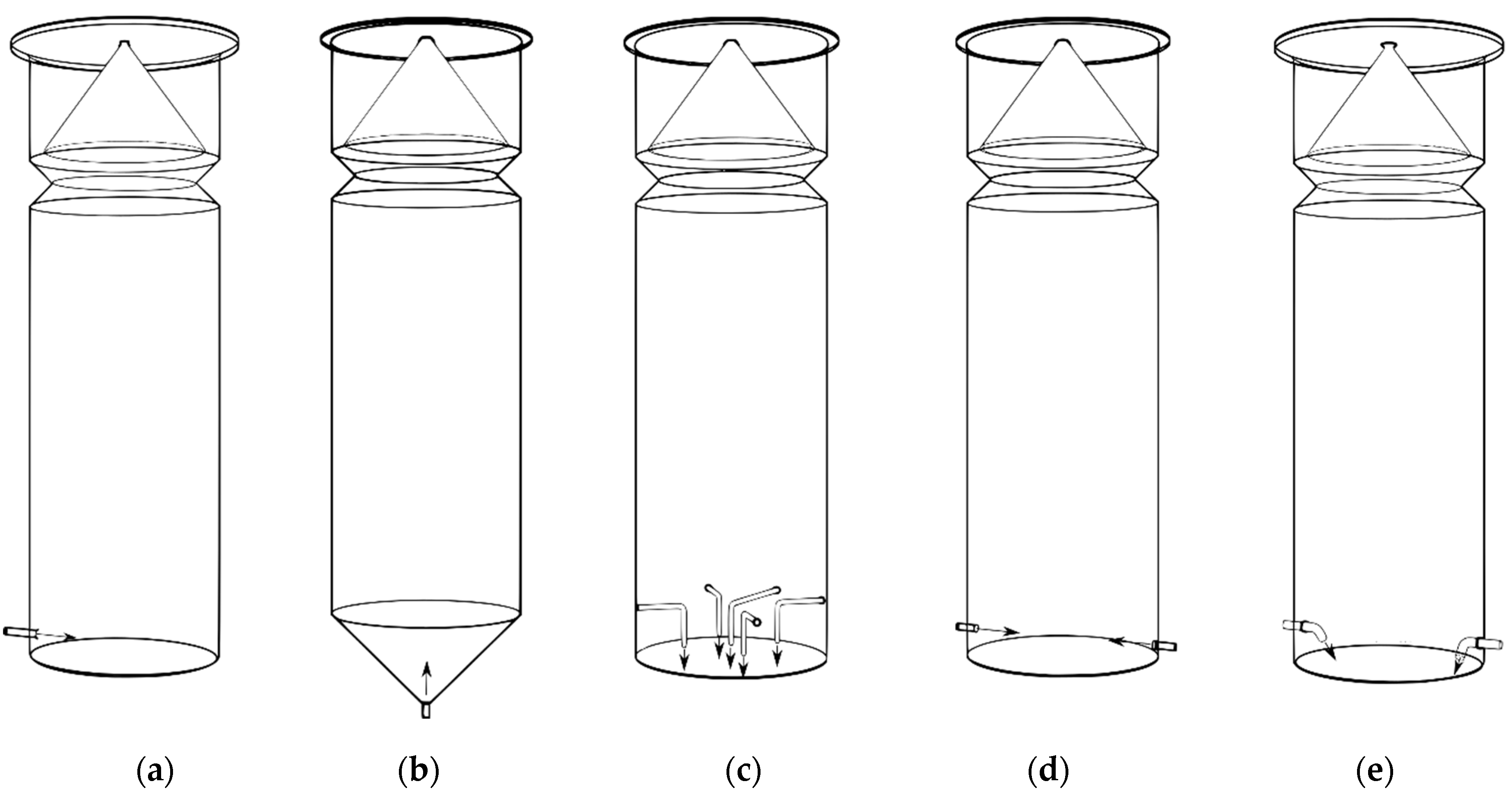
2.1. UASB Reactor

The cylindrical UASB reactor used herein was designed following the design guidelines by De Lemos Chernicharo [23] and Bressani-Ribeiro et al. [22] and is sized to treat 1 L/s of low-strength wastewater. The height and diameter of the reactor are 8.1 m and 2.5 m, respectively, providing a total effective volume of approximately 41 m³ and a hydraulic residence time (${\tau }_p$) of approximately 12 h. The reactor has a conical gas-liquid-solid separator (GLSS), a gas baffle, and an external gutter for treated water collection, as shown in Figure 1. This reactor has yet to be built as it is intended to use a model-based design approach to evaluate and optimize its IDS. Thus, the primary purpose of the reactor’s design is to evaluate the effect of five different IDS configurations on the global hydrodynamics of the reactor, which are expected to impact on the granular sludge development process. The evaluated configurations are depicted in Figure 2 and include (a) a single radial inflow configuration (C1), formed by a single lateral inlet pipe located at the bottom of the reactor, which is used in studies by Moawad et al. [39] and Singh et al. [40], (b) an upward axial inflow configuration (C2), consisting of a single inlet pipe located in the vertex of the conical base, similar to that used by Wu and Chen [41] and Das et al. [1], (c) a downward distributed inflow configuration (C3) that is formed by 5 inlet pipes pointing the water towards the bottom of the reactor. This configuration complies with UASB reactor design guidelines by De Lemos Chernicharo [23] and is applied in the study by Bastiani et al. [42]. (d) The opposite radial inflow configuration (C4), is formed by two inlet pipes pointing towards each other at the bottom of the reactor; and, (e) the tangential downward inflow configuration (C5), which is formed by two pipes ejecting water tangentially to the wall towards the bottom of the reactor at an angle of 45°. These two IDS are novel configurations proposed by the authors and were designed based on the idea that the water inlets should produce the highest turbulence in the reaction zone. This turbulence would generate an intensive mixing of substrate and nutrients with the biomass and minimize flow short-circuiting and dead zones. The turbulence must be quickly dissipated as the flow moves upward to allow the proper generation of the granular biomass. The proposed IDS designs also attempt to reduce the complexity of the operation, construction, maintenance, and use of materials. The five configurations were used in the simulations to evaluate the one that could benefit the hydrodynamics of the reactor in a better way and, therefore, its efficiency.

The global reactor’s Reynolds number (Re) is calculated using Equation (1), where $\rho$ and $\mu$ are the density $\left(998.8 \mathrm{kg}/{\mathrm{m}}^3\right)$ and dynamic viscosity of the fluid $\left(1.08\times {10}^{-3} \mathrm{kg}/\mathrm{m} \mathrm{s}\right)$, $Q$ is the flow rate of the reactor, and $D$ is the diameter of the reactor. The resulting Re is close to 450, which indicates that the overall regime of the reactor is laminar.

$$Re=\frac{4\rho Q}{\mu \pi D}$$

(1)

Equation (2) is used to estimate the jet Reynolds number (Re_j) [43] for the water inlets in each case. Where $u$ represents the velocity of the jet flow, and $D_j$ is the diameter of the water discharge pipe. The inlet jet Reynolds numbers for each case are presented in

Table 1. Jet Reynolds number of evaluated IDS configurations.

Parameter	IDS Configuration
	C1	C2	C3	C4	C5
Number of water inlets	1	1	5	2	2
Diameter of water inlet (mm)	114	114	72	72	72
Jet Reynolds number $\left(R{e}_j\right)$	10,036	10,036	3178	7945	7945

.

$$R{e}_j=\frac{\rho u{D}_j}{\mu }$$

(2)

2.2. Laboratory Scale Reactor

The geometry of the IDS configuration C1 (Figure 2a) was used to build a laboratory-scale reactor in order to validate the CFD simulations. The use of a laboratory-scale model is an approach often taken when full-scale reactor hydrodynamic data is not available. The configuration C1 was chosen because it is the most unfavorable IDS configuration among the five shown in Figure 2. This configuration generates the jet flow with the highest $R{e}_j$ among the evaluated IDS. In addition, the turbulence generated by the jet dissipates rapidly to a laminar regime as the flow moves upward after colliding the opposite wall of the reactor. The flow patterns generated by this configuration are particularly challenging for CFD simulation and are, therefore, suitable for validation purposes.

The dimensions of the laboratory-scale reactor were obtained using the dynamic similitude of Froude following the recommendations of Jamadi and Alighardashi [44]. The Froude dimensionless number was chosen since the cylindrical UASB reactor is considered an open hydraulic structure. Therefore, the forces that have the most significant influence on its hydraulic behavior are inertia and gravity [45]. The applied geometric similitude ratio was $\lambda =l_p/l_m=30.4$, obtaining a velocity and time ratio of $u_p/u_m=\sqrt{\lambda }=t_p/t_m=5.5$, where $l$ refers to the length, $t$ to the time, $u$ to the velocity. The subscripts $p$ and $m$ refer to the dimensions of the full-scale reactor and the laboratory-scale model, respectively. The laboratory-scale reactor was made of transparent LDPE with an internal diameter of 84 mm and a height of 267 mm, with an effective volume of approximately 1.45 L, as described in Cisneros et al. [28].

2.3. Tracer Tests

In order to obtain the residence time distribution (RTD) curve for the CFD validation, tracer tests were performed in the laboratory scale reactor using the stimulus-response pulse technique [46]. For the tests, the inflow in the scaled reactor was maintained at a constant rate of 12.0 ± 0.2 mL/min, obtaining a theoretical hydraulic retention time (${\tau }_m$) of approximately 2.15 h. Sodium chloride (NaCl) solution (Fisher Scientific, Loughborough, UK, CAS 7647-14-5 reagent grade) at a concentration of 1500 mg/L was employed as the tracer. The recommendations and the hardware of the automated tracer testing system presented by Cisneros et al. [28] were used to perform the tracer tests in this study. The specific conductance values were converted to NaCl concentrations by applying a calibration curve whose determination coefficient was $R^2\cong 0.99$. The tests were conducted until the recovery of the tracer reached at least 95%. All experiments were performed under laboratory conditions at a temperature of 17.5 °C ± 0.5 °C.

2.4. CFD Study

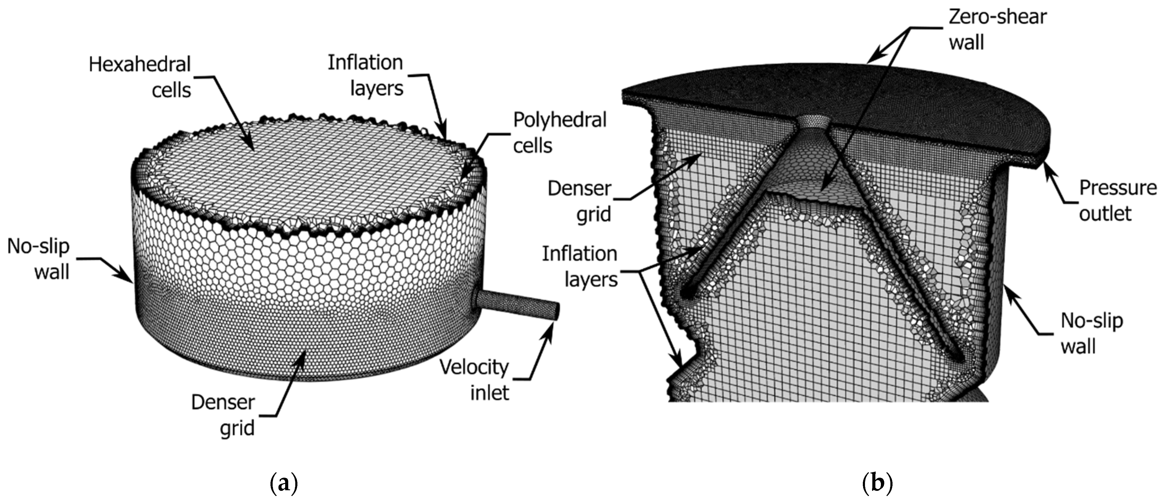
2.4.1. Domain Discretization and CFD Simulation

Fluent Meshing (ANSYS, Canonsburg, PA, USA) was used to generate poly-hexcore based unstructured grids from the 3D geometries shown in Figure 2a–e. Poly-hexcore grids combine poly prismatic elements with hexahedral elements whose interfaces are filled with polyhedral cells (Figure 3a,b). This grid type was chosen because it requires up to 40% fewer elements and speeds up the simulation convergence by 14% to obtain the same accuracy as alternative grid types [47]. Grid densities were intentionally increased in the water inlet and outlet zones and where flow separation occurs (i.e., GLSS base and gas baffle) using proximity and curvature functions, as seen in Figure 3a,b. Since the flow separation from the reactor walls can have a relevant effect on the overall hydrodynamics of the reactor [48], the viscous sublayer was resolved in the CFD simulations. Thus, inflation layers were included in the reactor walls to maintain a dimensionless wall distance magnitude $y^{+}~1$. The enhanced wall treatment option was enabled to maintain a $y^{+}$ insensitive wall treatment for the $\epsilon$-based turbulence model.

Single-phase, isothermal CFD simulations were performed using Fluent 19.5 (ANSYS, Canonsburg, PA, USA). Only the liquid phase was simulated in this study since it adequately represents the flow within the reactor during its start-up stage, as mentioned in Section 1. Understanding how different IDS configurations affect the hydraulic behavior of the reactor during this stage is critical for generating the conditions for improving granular sludge production. The simulated liquid was assumed to be incompressible and had Newtonian behavior with a density of 998.8 kg/m³ and a dynamic viscosity of 1.08 × 10⁻³ kg/m∙s. These conditions are considered realistic, assuming that the concentration of suspended solids during the start-up stage of a UASB reactor treating low-concentration wastewater is in the order of 30 mg/L. According to Vesvikar and Al-Dahhan [49], these characteristics provide a good approximation for anaerobic reactor modeling purposes. The boundary conditions for the simulations are detailed in

Table 2. CFD boundary conditions.

Boundary	Type	Unit	IDS Configuration
			C1 and C2	C3	C4 and C5
Water inlet	Velocity inlet	m/s	0.095	0.048	0.12
Water outlet	Pressure outlet	Pa	0	0	0
Reactor wall	No-slip wall	-	-	-	-
GLSS wall	No-slip wall	-	-	-	-
Water surface	Zero-shear wall	-	-	-	-

.

The pressure-velocity coupling for the numerical solution was performed as per the Semi-Implicit Method for Pressure Linked Equations (SIMPLE) [50]. The least-squares cell-based scheme was applied to calculate gradients, scalar values on cell faces, and velocity derivatives. This scheme provides substantial computational savings while maintaining high precision in the results [51]. The second-order upwind scheme was used for the spatial discretization to obtain greater accuracy in the results. The convergence of the simulations was judged based on monitoring the residuals and solution imbalances until reaching a value lower than 10 × 10⁻⁶. Velocity and pressure checkpoints were also included as local monitors for convergence evaluation. The simulations were run on a 6-core 2.9 GHz 64 GB Xeon workstation.

The Grid Convergence Index (GCI) [52] was used to obtain the discretization error of the CFD simulation. The GCI method involves running simulations on successively smaller grids to determine the error band of how far the calculated value of a quantity of interest is from its asymptotic value when using a hypothetical zero-space grid, which is estimated using Richardson’s extrapolation technique [53]. The Peclet number (Pe), the hydraulic residence time (HRT), and the peak of the RTD curve $E{\left(\theta \right)}_{peak}$ were employed as global performance parameters. The simulated flow velocity $\left(v\right)$ in the middle of the reactor, at 0.5 m from the bottom, was also used as a local performance parameter for the grid convergence study. A discretization error < 5% was considered adequate for this study to obtain representative results of the reactor’s behavior at a reasonable computational cost.

2.4.2. Governing Equations

The flow was solved using the mass and moment conservation equations presented in Equations (3) and (4).

$$\nabla ·\overrightarrow{v}=0$$

(3)

$$\frac{\partial }{\partial t}\left(\rho \overrightarrow{v}\right)+\nabla ·\left(\rho \overrightarrow{v}\overrightarrow{v}\right)=-\nabla p+\nabla ·\left(\stackrel{=}{\tau }\right)+\rho \overrightarrow{g}$$

(4)

$$\stackrel{=}{\tau }=\mu \left(\nabla \overrightarrow{v}+\nabla {\overrightarrow{v}}^T\right)$$

(5)

where $p$ is the static pressure, $\stackrel{=}{\tau }$ the shear stress tensor (Equation (5)), $\overrightarrow{g}$ the gravitational acceleration vector, $\overrightarrow{v}$ the fluid velocity vector, and $t$ the time.

In order to reduce the computational cost to describe the turbulent flow within the UASB reactor as accurately as possible, the performance of two RANS turbulence closure models was tested. The realizable k-epsilon model and the SST k-omega model were chosen due to their high performance to simulate the free-flow region and the possible incidence of boundary layers in the global hydrodynamics of the reactor. The performance of these turbulence models to reproduce the RTD curve from the laboratory scale reactor was verified using the Nash–Sutcliffe efficiency index (see Section 2.5).

• Realizable k-epsilon Model

The realizable k-epsilon model [54] is a robust, low computational cost, semi-empirical model that can be used to simulate a wide range of turbulent flows. It offers better performance than the standard version to solve rotating flows, boundary layer flows, and free flows with jets and mixing layers [51]. The transport equation to estimate the turbulence kinetic energy $\left(k\right)$ is shown in Equation (6). This model overcomes a deficiency of the standard model by solving the round jet anomaly by using a modified equation to estimate the turbulent dissipation rate $\left(\epsilon \right)$ (Equation (7)).

$$\frac{\partial }{\partial t}\left(\rho k\right)+\frac{\partial }{\partial x_j}\left(\rho k{u}_j\right)=\frac{\partial }{\partial x_j}\left[\left(\mu +\frac{{\mu }_t}{{\sigma }_k}\right)\frac{\partial k}{\partial x_j}\right]+G_k+G_b-\rho \epsilon$$

(6)

$$\frac{\partial }{\partial t}\left(\rho \epsilon \right)+\frac{\partial }{\partial x_j}\left(\rho \epsilon u_j\right)=\frac{\partial }{\partial x_j}\left[\left(\mu +\frac{{\mu }_t}{{\sigma }_{\epsilon }}\right)\frac{\partial \epsilon }{\partial x_j}\right]+\rho C_{1}S\epsilon -\rho C_2\frac{{\epsilon }^2}{k+\sqrt{\nu \epsilon }}+C_{1\epsilon }\frac{\epsilon }{k}{C}_{3\epsilon }{G}_b$$

(7)

where $u_j$ is the velocity component in the corresponding direction, ${\mu }_t$ represents eddy viscosity, $G_k$ and $G_b$ are the turbulence kinetic energy generation due to mean velocity gradients and buoyancy, respectively. $C_{1\epsilon }$, $C_{2\epsilon }$, $C_{3\epsilon }$ are constants of the model. ${\sigma }_k$ and ${\sigma }_{\epsilon }$ are the turbulent Prandtl numbers for $k$ and $\epsilon$, respectively. $S$ represents the modulus of the mean rate-of-strain tensor.

• SST k-omega Model

The Shear-Stress Transport (SST) k-omega model developed by Menter [55] is a turbulence closure model that combines the excellent performance of the omega and epsilon-based models in the viscous sublayer and in the free-flow region, respectively, using a blend function [51]. The transport equations that describe the turbulence kinetic energy (k) and the specific dissipation rate ($\omega$) are presented in Equations (8) and (9), respectively. In these equations $G_{\omega }$ is the generation of $\omega$, $Y_k$ and $Y_{\omega }$ represent the turbulence dissipation terms for $k$ and $\omega$, $D_{\omega }$ the cross-diffusion term and, ${\Gamma }_k$ and ${\Gamma }_{\omega }$ the effective diffusivity [53].

$$\frac{\partial }{\partial t}\left(\rho k\right)+\frac{\partial }{\partial x_i}\left(\rho k{u}_i\right)=\frac{\partial }{\partial x_j}\left({\Gamma }_k\frac{\partial k}{\partial x_j}\right)+G_k-Y_k$$

(8)

$$\frac{\partial }{\partial t}\left(\rho \omega \right)+\frac{\partial }{\partial x_i}\left(\rho \omega u_i\right)=\frac{\partial }{\partial x_j}\left({\Gamma }_{\omega }\frac{\partial \omega }{\partial x_j}\right)+G_{\omega }-Y_{\omega }+D_{\omega }$$

(9)

The blend function (Equation (10)) depends on the distance to the next surface $y$ (Equations (11)) and the positive portion of the cross-diffusion term $D_{\omega }^{+}$ (Equation (12)). This function modifies the Prandtl numbers ${\sigma }_k$ and ${\sigma }_{\omega }$ (Equations (13) and (14)) and thus the effective diffusivity ${\Gamma }_k$ and ${\Gamma }_{\omega }$ (Equations (15) and (16)).

$$F_1=tanh\left({\varphi }_1^4\right)$$

(10)

$${\varphi }_1=min\left[max\left(\frac{\sqrt{k}}{0.09\omega y},\frac{500\mu }{\rho y^2\omega }\right),\frac{4\rho k}{{\sigma }_{\omega ,2}{D}_{\omega }^{+}{y}^2}\right]$$

(11)

$$D_{\omega }^{+}=max\left[2\rho \frac{1}{{\sigma }_{\omega ,2}}\frac{1}{\omega }\frac{\partial k}{\partial x_j}\frac{\partial \omega }{\partial x_j},{10}^{-10}\right]$$

(12)

$${\sigma }_k=\frac{1 }{\frac{F_1}{{\sigma }_{k,1}}+\frac{1-F_1}{{\sigma }_{k,2}}}$$

(13)

$${\sigma }_{\omega }=\frac{1 }{\frac{F_1}{{\sigma }_{\omega ,1}}+\frac{1-F_1}{{\sigma }_{\omega ,2}}}$$

(14)

$${\Gamma }_k=\mu +\frac{{\mu }_t}{{\sigma }_k}$$

(15)

$${\Gamma }_{\omega }=\mu +\frac{{\mu }_t}{{\sigma }_{\omega }}$$

(16)

The eddy-viscosity is limited during the calculation of the turbulent shear stress (Equation (17)), where ${\alpha }^{*}$ is the low-Reynolds number correction coefficient, and $F_2$ is given by Equations (18) and (19) [51].

$${\mu }_t=\frac{\rho k}{\omega }\frac{1}{max\left[\frac{1}{{\alpha }^{*}},\frac{S{F}_2}{a_1\omega }\right]}$$

(17)

$$F_2=tanh\left({\mathsf{\Phi }}_2^2\right)$$

(18)

$${\mathsf{\Phi }}_2=max\left[2\frac{\sqrt{k}}{0.09\omega y},\frac{500\mu }{\rho y^2\omega }\right]$$

(19)

2.4.3. Species Transport

The stimulus-response pulse technique [46] was used to obtain the RTD curves employed to characterize the different IDS configurations’ influence on the UASB reactor’s hydrodynamics. During the CFD simulations, 1500 mg/L of a tracer with a density of 1002 kg/m³ was injected into the reactor inlet for 120 s. Equation (20) presents the convection-diffusion expression employed to estimate $Y$ (i.e., the tracer local mass fraction). In this equation, $R$ represents the species production net rate through chemical reaction, and $\overrightarrow{J}$ is the tracer flux diffusion due to concentration and temperature gradients [51].

$$\frac{\partial }{\partial t}\left(\rho Y\right)+\nabla ·\left(\rho \overrightarrow{v}Y\right)=-\nabla ·\overrightarrow{J}+R+S$$

(20)

The mass diffusion expression is presented in Equation (21), where $D_m$ is the mass diffusion coefficient in the mixture, $D_T$ is the thermal diffusion coefficient, and $S{c}_t$ is the turbulent Schmidt number [51].

$$\overrightarrow{J}=-\left(\rho D_m+\frac{{\mu }_t}{S{c}_t}\right)\nabla Y-D_T\frac{\nabla T}{T}$$

(21)

2.5. Characterization Variables

In order to determine the hydraulic characteristics of the reactor with the different IDS configurations, the following characterization variables were estimated. The Morrill Dispersion Index $\left(MDI\right)$ (Equation (22)) was used to measure the dispersion of the tracer within the reactor [56]. It is computed by relating the 90 percentile $\left(P_{90}\right)$ to the 10 percentile $\left(P_{10}\right)$ of the cumulative tracer curve. The Morrill volumetric efficiency $\left(V_e\right)$ (Equation (23)) was employed to estimate the portion of the reactor volume that is actually being used [56]. The Short-Circuiting Index $\left(SCI\right)$ (Equation (24)), measures the mixing efficiency in a reactor, which can be affected by channeling, back mixing, or stagnant zones [57]. In Equation (24), $t_i$ represents the time in which the tracer is detected for the first time at the reactor outlet when generating the RTD curve; $\tau$ represents the theoretical hydraulic residence time of the full-scale reactor $\left({\tau }_p\right)$ or the laboratory scale (${\tau }_m$). The dead volume $(V_d)$ (Equation (25)) indicates the portion of the reactor volume that is not operational, due to poor flow distribution [58]. Moreover, in Equation (25), $\overline{t}$ is equal to the average normalized retention time of the reactor. The granulation volume fraction $(V_{gr})$ (Equation (26)) is estimated to determine the portion of the reactor’s reaction zone that meets the granulation criteria (i.e., where the upward flow velocities are between 0.5 and 6 m/h) [23]. Where, $V_g$ represents the volume of granulation calculated by adding the cells’ volumes in the reaction zone of the CFD simulation that meet the granulation criteria. $V_R$ is the volume of the reaction zone.

The goodness of fit between the simulated RTD curves and those obtained from the tracer tests was estimated using the Nash-Sutcliffe efficiency $\left(NSE\right)$ index. The $NSE$ index can vary between $-\infty$ and 1, resulting in 1 when the fit between curves is perfect. Equation (27) was used to calculate the $NSE$ index, where $C_{Ot}$ is the concentration of the tracer at time $t$ measured in the physical model. $\overline{C_O}$ is the average concentration of the tracer during the entire test in the physical model and $C_{St}$ is the concentration of the tracer at time $t$ from the CFD simulation.

$$MDI=\frac{P_{90}}{P_{10}}$$

(22)

$$V_e=\frac{1}{MDI}$$

(23)

$$SCI=\frac{t_i}{\tau }$$

(24)

$$V_d=(1-\frac{\overline{t}}{\tau })\times 100$$

(25)

$$V_{gr}=\frac{V_g}{V_R}\times 100$$

(26)

$$NSE=1-\frac{{\sum }^{ }{\left(C_{Ot}-C_{St}\right)}^2}{{\sum }^{ }{\left(C_{Ot}-\overline{C_O}\right)}^2}$$

(27)

3. Results and Discussion

3.1. Grid Convergence Analysis

The IDS configuration C1 (Figure 2a) was selected to perform the grid convergence analysis. Three different quality grids were generated for this analysis: a coarse quality grid with 1,281,435 cells, a medium grid with 2,796,190, and a fine grid with 6,165,642 cells. The element size refinement ratios between the coarse and medium grid and between the medium and fine grid were approximately 1.3. For the transient simulation, time steps of 0.25, 0.20, and 0.15 s were used for the coarse, medium, and fine grids, respectively, to keep the Courant number below 0.8. The grids had average skewness values ranging from 0.03 to 0.06 (

Table 3. Grid quality and performance parameters.

Grid Quality	Grid			Performance Parameters
	Average Cell Size (m)	Refinement Ratio	Average Skewness	Pe	E(θ)peak	HRT	$\mathit{v}$
Fine	0.019	1.3	0.03	8.02	0.853	653.82	0.0069
Medium	0.024	1.3	0.04	7.97	0.850	654.53	0.0070
Coarse	0.032		0.06	7.55	0.822	659.56	0.0079
			RE	8.02	0.853	653.71	0.0069

Note: Pe—Peclet number; E(θ)_peak—tracer dimensionless concentration peak; HRT—hydraulic residence time (min); $v$—local flow velocity (m/s); RE—Richardson extrapolation.

), indicating that the poly-hexcore based grid provides exceptional quality [51] for CFD simulation. The performance parameters shown in this table became asymptotic as the size of the grid cell decreased, approaching Richardson’s extrapolation values, which is a sign of monotonic convergence.

The local flow velocity is the performance parameter that generates the highest GCI values for all cases, with a maximum of 16.62% for the coarse grid (

Table 4. Grid convergence index.

Grid Quality	GCI (%)
	Pe	E(θ)peak	HRT	$\mathit{v}$
Fine	0.117	0.031	0.021	0.129
Medium	0.951	0.380	0.156	1.495
Coarse	7.540	4.482	1.118	16.624
ARC	1.007	1.003	0.999	0.990

Note: Pe—Peclet number; E(θ)_peak—tracer dimensionless concentration peak; HRT—hydraulic residence time; $v$—local flow velocity (m/s); ARC—asymptotic range of convergence (unitless).

). On the global performance parameters, the calculation of the Peclet number is the one that produces the highest GCIs, with a maximum GCI of 7.54% for the coarse mesh. On the other hand, the HRT is the parameter with the lowest incidence on the GCI values with a maximum of 1.12% for the coarse grid and 0.02% for the fine grid. All performance parameters in the evaluated grids reached an Asymptotic Range of Convergence $\left(ARC\right)$ value of approximately 1. The medium-quality grid was chosen to perform the rest of the simulations in this study because it offered the quality required to estimate the performance parameters with an error within the expected range (see Section 2.4.1) at the lowest computational cost.

Since the IDS configuration C1 has the most unfavorable conditions for CFD simulation (due to its complex flow patterns and high jet Reynolds number), the discretization errors of the remaining IDS configurations are assumed to be less than those obtained in Table 4.

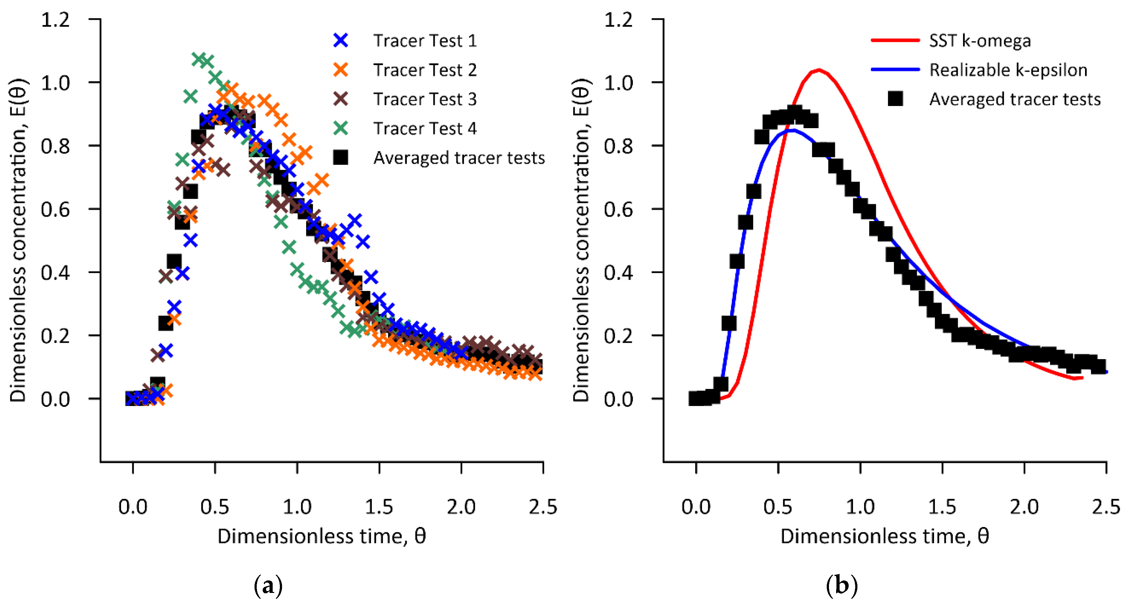
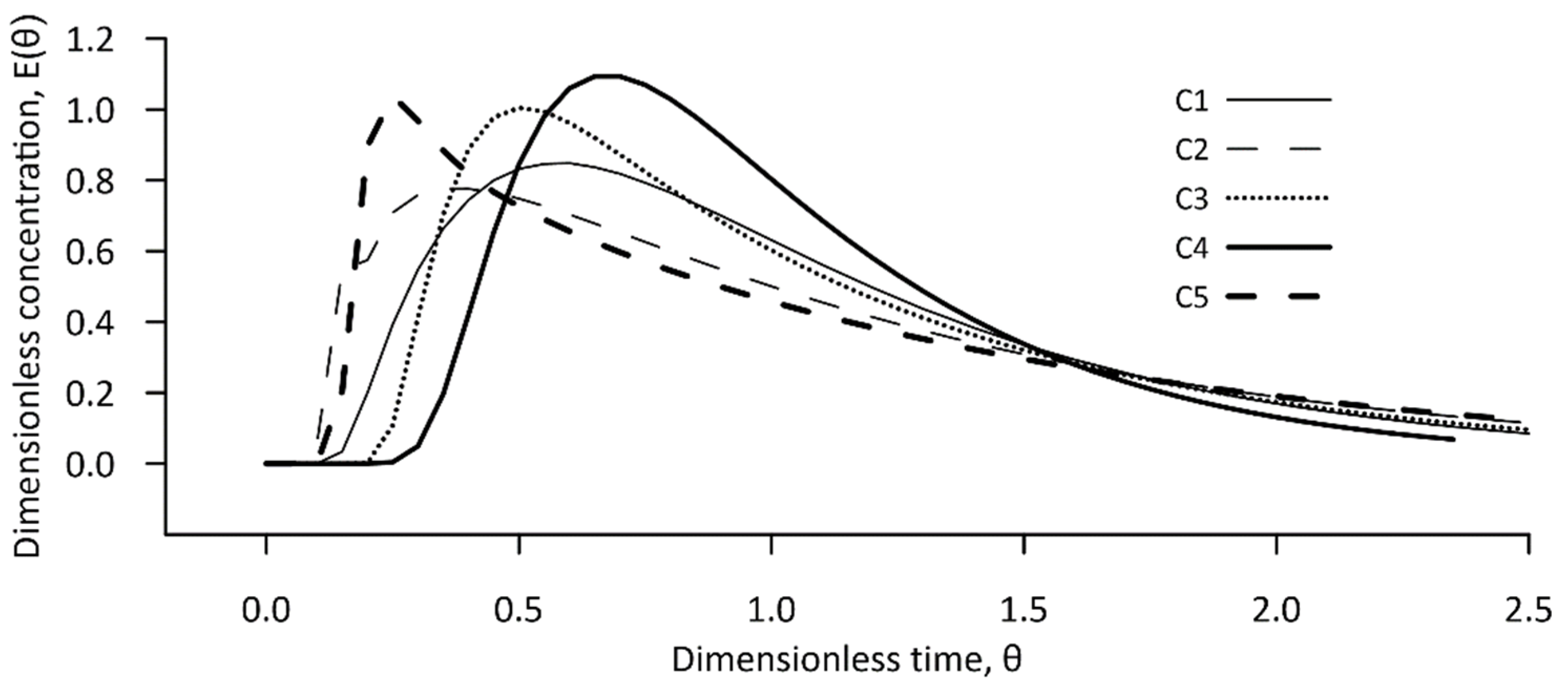
3.2. Tracer Test and Selection of the Turbulence Model

Four tracer tests were conducted to characterize the hydrodynamic behavior of the UASB reactor using a hydraulically scaled physical model (laboratory-scale reactor). The RTD curves resulting from these tests are presented in Figure 4a. Despite the data dispersion among the obtained RTD curves, their shapes resemble the response of a tank reactor with dead zones and channeling, which is the expected response of a UASB reactor [59]. The dispersion of data among the four tracer tests can be attributed to flow instabilities in the reactor due to dead zones, channeling, and short-circuiting. Although the geometry of the reactor has a relevant impact on these effects, the greatest impact is produced by inlet jet flow, which, being an inherently turbulent structure [60] chaotically influences the surrounding region [28].

An averaged RTD curve of the four tracer tests (Figure 4a) was calculated to obtain a representative RTD curve of the behavior of the UASB reactor flow. The averaged RTD curve shows a fast tracer output and a tracer peak $E{\left(\theta \right)}_{peak}=0.91\pm 0.04$ at $\theta \cong 0.60$ evidencing the presence of flow short-circuiting [46]. Larger deviations on the tracer measurements from the mean were found at $\theta \cong 1.25$ reaching a magnitude close to $0.14$. The averaged RTD curve was also used to validate the performance of the turbulence models used in this study. The degree of similarity of the CFD simulated RTD curves and the tracer averaged RTD curve are $NSE=0.98$ for the realizable k-epsilon model and $NSE=0.68$ for the SST k-omega model. A value $NSE=1$ indicates that the CFD simulation perfectly represents the global hydrodynamic behavior of the reactor. Therefore, the high $NSE$ obtained by the epsilon-based turbulence model suggests that it is appropriate to use it in this characterization study. Figure 4b confirms that the fit of the RTD curve generated by the realizable k-epsilon model to the averaged RTD curve of the tracer tests is better than that generated by the SST k-omega model. The fit weakens only in two small regions of the curve, near its peak at $\theta \cong 0.60$ and $\theta \cong 1.50$, where the slope of the averaged RTD curve changes abruptly. These minor shortcomings do not invalidate the excellent prediction of the realizable k-epsilon model. Thus, this model was used through the rest of the simulations in this study.

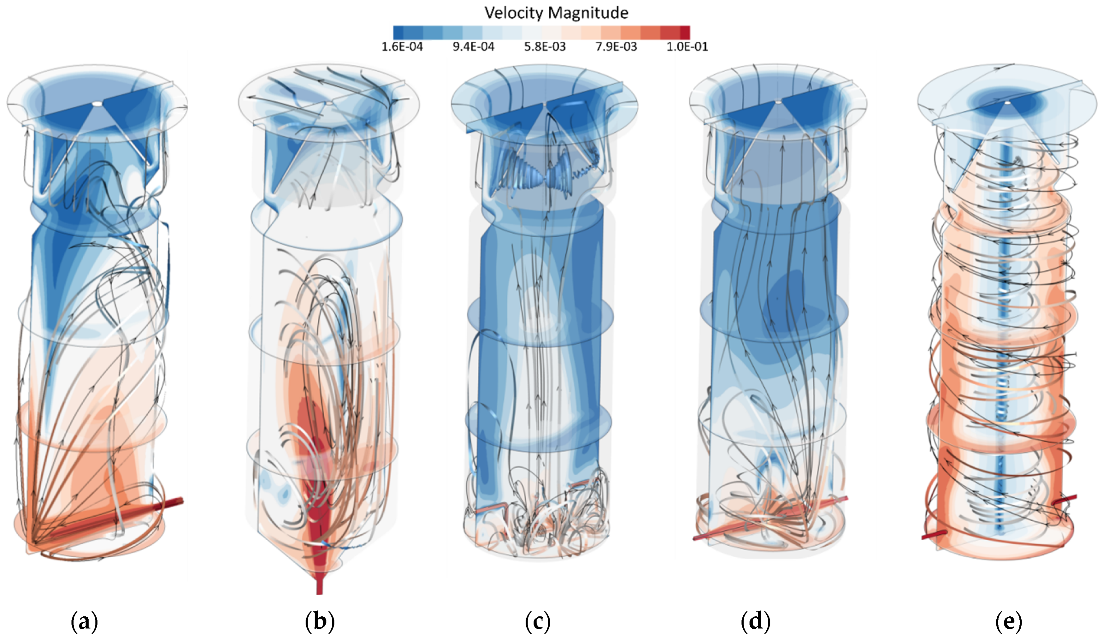
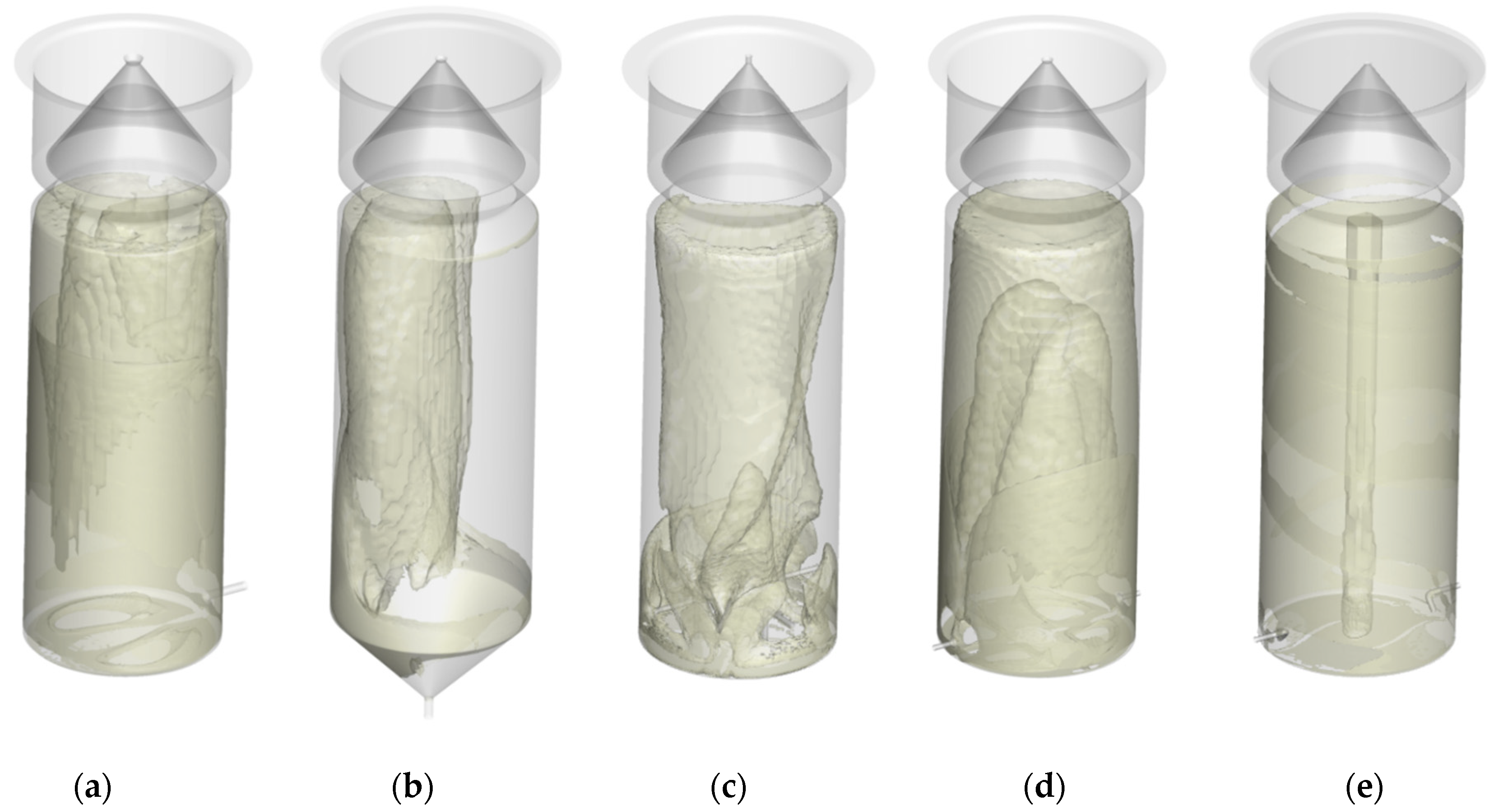
3.3. IDS Performance

Five CFD simulations were conducted to characterize the hydrodynamics of a cylindrical UASB reactor with different IDS configurations (C1 to C5). One of the most important parameter was the velocity distribution in the reactor’s reaction zone (Figure 5a–e). This zone is crucial for granule formation, as it provides the necessary shear force to remove the lighter particles from the growth nuclei (see Section 1).

The velocity contours of IDS C1 (Figure 5a) show a marked jet flow reaching the wall opposite the flow inlet. The jet flow rapidly dissipates its energy during this path, as the jet velocity decreases by approximately 84%. The flow patterns depicted in the figure as ribbons show that a broad circular pattern is formed, occupying a large volume of the reactor’s reaction zone. Similarly, the velocity contours of the IDS C2 (Figure 5b) show a rapidly dissipating jet flow pattern. The indicator ribbons show that the flow lines develop in ascending and descending circular patterns until the flow finally exits the reactor. Figure 5c shows that IDS C3 allows a relevant energy dissipation at the bottom of the reactor, forming fairly compact circular patterns compared to the cases previously analyzed. In this configuration, a clear upward flow pattern is found in the central zone of the reactor, which confirms the reasons why this IDS is recommended on the design guidelines [10,22,23,24]. Figure 5d shows the flow velocity distribution of IDS C4. In this case, a high dissipation of energy in the central zone of the bottom of the reactor is produced. As in IDS C3, a clear upward flow pattern is generated, indicating that this configuration may be suitable for an effective granulation process. The jet flows generated by the water outlets in the IDS C5 dissipate rapidly upon hitting the bottom of the reactor, forming a very complex upward and downward spiral flow pattern (Figure 5e). Very low flow velocity zones appear in the reactor (shown in blue in Figure 5a–e), especially inside and above the GLSS, which could be considered stagnant zones. These zones will negatively affect the effective volume of the reactor.

The granulation zone of a UASB reactor (i.e., the zone where the recommended upward flow velocities for the granulation process are met) is neither uniform nor compact since the flow patterns that form it depend significantly on the IDS configuration. Using CFD tools, it is possible to determine the granulation zone and estimate its volume. In theory, the larger the granulation volume, the greater the potential to form granules and, therefore, the shorter the reactor start-up stage. Thus, it is possible to establish the most favorable IDS configuration for the granulation process to occur.

Figure 6a–e shows the granulation volumes generated by the IDS configurations (C1–C5). The granulation volume produced by IDS C1 (Figure 6a) shows that the potential granule production zone is located near the wall opposite the flow inlet, with a $V_{gr}=11.8\%$. A granulation volume with a relatively similar magnitude $\left(V_{gr}=10.8\%\right)$ is formed by the IDS C2 (Figure 6b). Although in both cases it is seen that the granulation volume is reduced, both IDS configurations are commonly used in operational UASB reactors [1,41,61,62]. Low granulation in these regions could explain the long periods of time required in the start-up stage of the UASB reactor that are reported frequently [16,23]. Moreover, the IDS configuration C2 is used in previous works reporting hydraulic and treatment efficiencies [36,63]. However, the configuration recommended by the UASB reactor design guidelines (IDS C3), with a $V_{gr}=37.2\%$, has a marked superiority to form a greater granulation volume (Figure 6c) than the C1 and C2 IDS configurations. Nevertheless, the novel IDS configuration C4 generates the highest granulation volume of all the evaluated IDS (Figure 6d), $V_{gr}=45.5\%$, which is 22.4% higher than that of the configuration IDS C3. Furthermore, the flow pattern produced by IDS C5 generates the concentrated granulation volume in the middle of the reactor shown in Figure 6e with a $V_{gr}=21.4\%$.

Based on the MDI (

Table 5. Hydrodynamic characterization of UASB with different IDS configurations.

IDS Configuration	MDI	${\mathit{V}}_{\mathit{e}}(\%)$	Pe	SCI	${\mathit{V}}_{\mathit{d}}(\%)$
C1	4.71	21.23	7.96	0.11	7.8
C2	7.08	14.12	6.56	0.06	14.2
C3	4.37	22.88	7.97	0.17	6.8
C4	3.20	31.23	10.50	0.21	0.8
C5	7.65	13.07	6.31	0.10	16.4

Note: MDI—Morrill Dispersion Index; V_e—Morrill volumetric efficiency; Pe—Peclet number; SCI—Short-Circuiting Index; V_d—dead volume.

), the IDS C5 has the lowest Morrill volumetric efficiency, with $V_e=13.07\%$, followed closely by IDS C2, with $V_e=14.12\%$, while the highest is IDS C4 with $V_e=31.23\%$. These results indicate that IDS C4 is the one that produces a response in the reactor flow that most resembles a plug flow. The lowest $SCI$ is generated by IDS C2 with $0.06$ (Table 5), which indicates that the tracer leaves the reactor prematurely due to the presence of flow short-circuiting. This phenomenon is understandable due to the opposite location of the water inlet and outlet in this configuration. IDS C4 produced a $SCI=0.21$, the highest among of all IDS systems analyzed, suggesting that the tracer mixing in the reactor is much more intense, which brings the tracer exit time closer to the theoretical hydraulic retention time of the reactor. IDS C2 and C5 have the highest $V_d$ with $14.2\%$ and $16.4\%,$ respectively (Table 5). In IDS C5, the base of the reactor acts as a restriction for the movement of the fluid when it leaves the distribution pipes, creating a rebound effect that limits the mixing of the tracer in the lower area, which avoids that an important fraction of the reactor works properly. The lowest $V_d$ is held by IDS C3 and C4 with $6.8\%$ and $0.8\%$, respectively. IDS C4 shows a considerable improvement in the use of the volume within the reactor that will have an additional benefit to produce granular sludge and probably for the overall efficiency of the reactor. In Table 5, the darkest highlight represents the most advantageous values and the lightest the most disadvantageous values.

The RTD curves generated by the CFD simulations are presented in Figure 7. The shape of these curves confirms the results shown in Table 4. A rapid tracer exit occurs especially for IDS C2 and C5, reaching $E{\left(\theta \right)}_{peak}\cong 0.78$ at $\theta \cong 0.40$ and $E{\left(\theta \right)}_{peak}=1.04$ at $\theta \cong 0.25$, respectively, indicating the presence of stagnant zones and short-circuiting [46]. As a result of these flow limitations, both IDS configurations would produce a faulty reactor mix that could significantly affect the efficiency of the reactor treatment by affecting the proper distribution of nutrients and substrate to the granular biomass. Flow short-circuiting occurs in IDS configurations C1, C3, and C4, to a lesser extent, which shows that mixing is much more efficient in these three configurations. IDS C3 and C4 generate better flows than the rest of the studied IDS, with IDS C3 reaching $E{\left(\theta \right)}_{peak}\cong 1.0$ at $\theta \cong 0.50$ and IDS C4 $E{\left(\theta \right)}_{peak}\cong 1.09$ at $\theta \cong 0.70$.

The results indicate the superiority of IDS C3 to conduct the granulation process compared to conventional IDS. However, IDS C4 generates 22.4% more granulation volume within the reaction zone. The reactor volumetric efficiency increases by 36.5%, the flow short-circuiting is reduced by 19.8%, and the reactor dead volume is reduced by 88.2% compared to IDS C3. Although this novel configuration needs to be tested in the field, it appears to be a promising IDS configuration. In addition to the benefits regarding the hydrodynamic behavior of the flow, its implementation would be simpler and cheaper since it consists of only two external pipes. Using external pipes to inject the water into the rector would considerably reduce the blockages that occasionally occur in the water inlet pipes in IDS C3 [23], minimizing the costs of operation and maintenance of the reactor.

4. Conclusions

CFD simulations performed on a cylindrical UASB reactor confirm that the IDS configuration directly impacts the hydrodynamics of the reactor and its hydraulic efficiency. The IDS configurations simple radial inflow (C1), upward axial inflow (C2), downward distributed inflow (C3), opposite radial inflow (C4), and downward tangential inflow (C5) were evaluated in this study to determine their influence on the granulation volume of the reactor. The realizable k-epsilon model was used as a turbulence closure model in the CFD simulation after a validation process on a physical model with Froude dynamic similitude. The validation process obtained a $NSE=0.98$ indicating the high representativeness of the CFD model. Results indicate that the most unfavorable IDS configurations for granulation are IDS C2 and C5, with a relative granulation volume of 13.07% and 14.12%, respectively. The most favourable IDS configurations are C3 and C4, with a relative granulation volume of 31.23% and 22.88%, respectively. IDS C4 has a granulation volume 22.4% greater than the recommendation of the design guidelines for UASB reactors (IDS C3). This improvement in the granulation volume suggests that IDS C4 can reduce rector start-up time and possibly increase its treatment efficiency. Further studies could help analyze whether the gradual formation of granules during the reactor start-up stage can affect the granulation volume of CFD simulations by modifying the flow patterns within the UASB reactor with different IDS configurations.

References

1. Das, S.; Sarkar, S.; Chaudhari, S. Modification of UASB Reactor by Using CFD Simulations for Enhanced Treatment of Municipal Sewage. Water Sci. Technol. 2017, 77, 766–776. [Google Scholar] [CrossRef]
2. Das, S.; Chaudhari, S. Effect of Reactor Configuration on Performance during Anaerobic Treatment of Low Strength Wastewater. Environ. Technol. 2015, 36, 2312–2318. [Google Scholar] [CrossRef] [PubMed]
3. Singh, K.S.; Harada, H.; Viraraghavan, T. Low-Strength Wastewater Treatment by a UASB Reactor. Bioresour. Technol. 1996, 55, 187–194. [Google Scholar] [CrossRef]
4. Karim, K.; Varma, R.; Vesvikar, M.; Al-Dahhan, M.H. Flow Pattern Visualization of a Simulated Digester. Water Res. 2004, 38, 3659–3670. [Google Scholar] [CrossRef]
5. Von Sperling, M.; de Lemos Chernicharo, C. Biological Wastewater Treatment in Warm Climate Regions; IWA Publishing: London, UK, 2017; ISBN 978-1-78040-273-4. [Google Scholar]
6. UN DESA. Transforming Our World: The 2030 Agenda for Sustainable Development; United Nations Department of Economic and Social Affairs: New York, NY, USA, 2016. [Google Scholar]
7. Lettinga, G.; van Velsen, A.F.M.; Hobma, S.W.; de Zeeuw, W.; Klapwijk, A. Use of the Upflow Sludge Blanket (USB) Reactor Concept for Biological Wastewater Treatment, Especially for Anaerobic Treatment. Biotechnol. Bioeng. 1980, 22, 699–734. [Google Scholar] [CrossRef]
8. Latif, M.A.; Ghufran, R.; Wahid, Z.A.; Ahmad, A. Integrated Application of Upflow Anaerobic Sludge Blanket Reactor for the Treatment of Wastewaters. Water Res. 2011, 45, 4683–4699. [Google Scholar] [CrossRef]
9. De Lemos Chernicharo, C.A.; van Lier, J.B.; Noyola, A.; Ribeiro, T.B. Anaerobic Sewage Treatment: State of the Art, Constraints and Challenges. Rev. Environ. Sci. Biotechnol. 2015, 14, 649–679. [Google Scholar] [CrossRef]
10. Lettinga, G.; Pol, L.W.H. UASB-Process Design for Various Types of Wastewaters. Water Sci. Technol. 1991, 24, 87–107. [Google Scholar] [CrossRef]
11. Liu, Y.; Xu, H.-L.; Yang, S.-F.; Tay, J.-H. Mechanisms and Models for Anaerobic Granulation in Upflow Anaerobic Sludge Blanket Reactor. Water Res. 2003, 37, 661–673. [Google Scholar] [CrossRef]
12. Tay, J.-H.; Tay, S.T.-L.; Liu, Y.; Show, K.Y.; Ivanov, V. Biogranulation Technologies for Wastewater Treatment: Microbial Granules; Elsevier: Amsterdam, The Netherlands, 2006; ISBN 978-0-08-047608-7. [Google Scholar]
13. Batstone, D.J.; Keller, J. Variation of Bulk Properties of Anaerobic Granules with Wastewater Type. Water Res. 2001, 35, 1723–1729. [Google Scholar] [CrossRef]
14. Chang, Y.-J.; Nishio, N.; Nagai, S. Characteristics of Granular Methanogenic Sludge Grown on Phenol Synthetic Medium and Methanogenic Fermentation of Phenolic Wastewater in a UASB Reactor. J. Ferment. Bioeng. 1995, 79, 348–353. [Google Scholar] [CrossRef]
15. Hulshoff Pol, L.W.; de Castro Lopes, S.I.; Lettinga, G.; Lens, P.N.L. Anaerobic Sludge Granulation. Water Res. 2004, 38, 1376–1389. [Google Scholar] [CrossRef] [PubMed]
16. Show, K.-Y.; Yan, Y.; Yao, H.; Guo, H.; Li, T.; Show, D.-Y.; Chang, J.-S.; Lee, D.-J. Anaerobic Granulation: A Review of Granulation Hypotheses, Bioreactor Designs and Emerging Green Applications. Bioresour. Technol. 2020, 300, 122751. [Google Scholar] [CrossRef]
17. Noyola, A.; Moreno, G. Granule Production from Raw Waste Activated Sludge. Water Sci. Technol. 1994, 30, 339–346. [Google Scholar] [CrossRef]
18. Hulshoff Pol, L.W.; de Zeeuw, W.J.; Velzeboer, C.T.M.; Lettinga, G. Granulation in UASB-Reactors. Water Sci. Technol. 1983, 15, 291–304. [Google Scholar] [CrossRef]
19. Hulshoff Pol, L.W.; Heijnekamp, K.; Lettinga, G. The Selection Pressure as A Driving Force Behind The Granulation of Anaerobic Sludge. In Granular Anaerobic Sludge: Microbiology and Technology; Kluwer Wageningen: Alphen an den Rijn, The Netherlands, 1988; pp. 153–161. [Google Scholar]
20. McSwain, B.S.; Irvine, R.L.; Hausner, M.; Wilderer, P.A. Composition and Distribution of Extracellular Polymeric Substances in Aerobic Flocs and Granular Sludge. Appl. Environ. Microbiol. 2005, 71, 1051–1057. [Google Scholar] [CrossRef] [Green Version]
21. Hoffmann, R.A.; Garcia, M.L.; Veskivar, M.; Karim, K.; Al-Dahhan, M.H.; Angenent, L.T. Effect of Shear on Performance and Microbial Ecology of Continuously Stirred Anaerobic Digesters Treating Animal Manure. Biotechnol. Bioeng. 2008, 100, 38–48. [Google Scholar] [CrossRef] [PubMed]
22. Bressani-Ribeiro, T.; Chernicharo, C.A.L.; Lobato, L.C.S.; Neves, P.N.P. Design of UASB Reactors for Sewage Treatment. In Anaerobic Reactors for Sewage Treatment: Design, Construction, and Operation; Chernicharo, C.A.L., Bressani-Ribeiro, T., Eds.; IWA Publishing: London, UK, 2019. [Google Scholar]
23. De Lemos Chernicharo, C.A. Anaerobic Reactors; IWA publishing: London, UK, 2017. [Google Scholar]
24. Van Lier, J.B.; Vashi, A.; Van Der Lubbe, J.; Heffernan, B. Anaerobic Sewage Treatment using UASB Reactors: Engineering and Operational Aspects. In Environmental Anaerobic Technology; Imperial College Press: London, UK, 2010; pp. 59–89. ISBN 978-1-84816-542-7. [Google Scholar]
25. Yang, G.; Wang, J.; Zhang, H.; Jia, H.; Zhang, Y.; Gao, F. Applying Bio-Electric Field of Microbial Fuel Cell-Upflow Anaerobic Sludge Blanket Reactor Catalyzed Blast Furnace Dusting Ash for Promoting Anaerobic Digestion. Water Res. 2019, 149, 215–224. [Google Scholar] [CrossRef] [PubMed]
26. Ozgun, H.; Ersahin, M.E.; Zhou, Z.; Tao, Y.; Spanjers, H.; van Lier, J.B. Comparative Evaluation of the Sludge Characteristics along the Height of Upflow Anaerobic Sludge Blanket Coupled Ultrafiltration Systems. Biomass Bioenergy 2019, 125, 114–122. [Google Scholar] [CrossRef]
27. Singh, K.S.; Viraraghavan, T. Start-up and Operation of UASB Reactors at 20 °C for Municipal Wastewater Treatment. J. Ferment. Bioeng. 1998, 85, 609–614. [Google Scholar] [CrossRef]
28. Cisneros, J.F.; Pelaez-Samaniego, M.R.; Pinos, V.; Nopens, I.; Alvarado, A. Development of an Automated Tracer Testing System for UASB Laboratory-Scale Reactors. Water 2021, 13, 1821. [Google Scholar] [CrossRef]
29. Morgan-Sagastume, J.M.; Jiménez, B.; Noyola, A. Tracer Studies in a Laboratory and Pilot Scale UASB Reactor. Environ. Technol. 1997, 18, 817–825. [Google Scholar] [CrossRef]
30. Laurent, J.; Samstag, R.W.; Ducoste, J.M.; Griborio, A.; Nopens, I.; Batstone, D.J.; Wicks, J.D.; Saunders, S.; Potier, O. A Protocol for the Use of Computational Fluid Dynamics as a Supportive Tool for Wastewater Treatment Plant Modelling. Water Sci. Technol. 2014, 70, 1575–1584. [Google Scholar] [CrossRef]
31. Samstag, R.W.; Ducoste, J.J.; Griborio, A.; Nopens, I.; Batstone, D.J.; Wicks, J.D.; Saunders, S.; Wicklein, E.A.; Kenny, G.; Laurent, J. CFD for Wastewater Treatment: An Overview. Water Sci. Technol. 2016, 74, 549–563. [Google Scholar] [CrossRef] [PubMed]
32. Alvarado, A.; Vesvikar, M.; Cisneros, J.F.; Maere, T.; Goethals, P.; Nopens, I. CFD Study to Determine the Optimal Configuration of Aerators in a Full-Scale Waste Stabilization Pond. Water Res. 2013, 47, 4528–4537. [Google Scholar] [CrossRef] [PubMed]
33. Amaral, A.; Gillot, S.; Garrido-Baserba, M.; Filali, A.; Karpinska, A.M.; Plósz, B.G.; De Groot, C.; Bellandi, G.; Nopens, I.; Takács, I.; et al. Modelling Gas–Liquid Mass Transfer in Wastewater Treatment: When Current Knowledge Needs to Encounter Engineering Practice and Vice Versa. Water Sci. Technol. 2019, 80, 607–619. [Google Scholar] [CrossRef] [PubMed] [Green Version]
34. Tobo, Y.M.; Rehman, U.; Bartacek, J.; Nopens, I. Partial Integration of ADM1 into CFD: Understanding the Impact of Diffusion on Anaerobic Digestion Mixing. Water Sci. Technol. 2020, 81, 1658–1667. [Google Scholar] [CrossRef]
35. Souza, C.L.; Chernicharo, C.A.L.; Aquino, S.F. Quantification of Dissolved Methane in UASB Reactors Treating Domestic Wastewater under Different Operating Conditions. Water Sci. Technol. 2011, 64, 2259–2264. [Google Scholar] [CrossRef]
36. Wongnoi, R.; Songkasiri, W.; Phalakornkule, C. Influence of a Three-Phase Separator Configuration on the Performance of an Upflow Anaerobic Sludge Bed Reactor Treating Wastewater from a Fruit-Canning Factory. Water Environ. Res. 2007, 79, 199–207. [Google Scholar]
37. Kundu, P.; Mishra, I. CFD Modelling of an Uasb Reactor for Biogas Production from Industrial Waste/Domestic Sewage. In Recent Advances in Bioenergy Research; Sardar Swaran Singh National Institute of Renewable Energy: Kapurthala, India, 2013; Volume I, pp. 176–193. ISBN 978-81-927097-0-3. [Google Scholar]
38. Koerich, D.M.; Rosa, L.M. Optimization of Bioreactor Operating Conditions Using Computational Fluid Dynamics Techniques. Can. J. Chem. Eng. 2016, 95, 199–204. [Google Scholar] [CrossRef]
39. Moawad, A.; Mahmoud, U.F.; El-Khateeb, M.A.; El-Molla, E. Coupling of Sequencing Batch Reactor and UASB Reactor for Domestic Wastewater Treatment. Desalination 2009, 242, 325–335. [Google Scholar] [CrossRef]
40. Singh, K.S.; Viraraghavan, T.; Bhattacharyya, D. Sludge Blanket Height and Flow Pattern in UASB Reactors: Temperature Effects. J. Environ. Eng. 2006, 132, 895–900. [Google Scholar] [CrossRef]
41. Wu, B.; Chen, S. CFD Simulation of Non-Newtonian Fluid Flow in Anaerobic Digesters. Biotechnol. Bioeng. 2008, 99, 700–711. [Google Scholar] [CrossRef]
42. Bastiani, C.D.; Alba, J.L.; Mazzarotto, G.T.; de Farias Neto, S.R.; Reynolds, A.; Kennedy, D.; Beal, L.L. Three-Phase Hydrodynamic Simulation and Experimental Validation of an Upflow Anaerobic Sludge Blanket Reactor. Comput. Math. Appl. 2021, 83, 95–110. [Google Scholar] [CrossRef]
43. Revill, B.K. Chapter 9—Jet mixing. In Mixing in the Process Industries; Harnby, N., Edwards, M.F., Nienow, A.W., Eds.; Butterworth-Heinemann: Oxford, UK, 1992; pp. 159–183. ISBN 978-0-7506-3760-2. [Google Scholar]
44. Jamadi, M.H.; Alighardashi, A. Application of Froude Dynamic Similitude in Anaerobic Baffled Reactors to Prediction of Hydrodynamic Characteristics of a Prototype Reactor Using a Model Reactor. Water Sci. Eng. 2017, 10, 53–58. [Google Scholar] [CrossRef]
45. Streeter, V.; Wylie, B.; Bedford, K.W. Fluid Mechanics, 9th ed.; McGraw Hill Education: New York, NY, USA, 2010; ISBN 978-0-07-070140-3. [Google Scholar]
46. Levenspiel, O. Chemical Reaction Engineering, 3rd ed.; Wiley: New York, NY, USA, 1998; ISBN 978-0-471-25424-9. [Google Scholar]
47. Zore, K.; Caridi, D.; Lockley, I. Fast and Accurate Prediction of Vehicle Aerodynamics Using ANSYS Mosaic Mesh; SAE International: Warrendale, PA, USA, 2020. [Google Scholar]
48. Shi, W.; Wang, D.; Atlar, M.; Seo, K.-C. Flow Separation Impacts on the Hydrodynamic Performance Analysis of a Marine Current Turbine Using CFD. Proc. Inst. Mech. Eng. Part J. Power Energy 2013, 227, 833–846. [Google Scholar] [CrossRef]
49. Vesvikar, M.S.; Al-Dahhan, M. Flow Pattern Visualization in a Mimic Anaerobic Digester Using CFD. Biotechnol. Bioeng. 2005, 89, 719–732. [Google Scholar] [CrossRef] [PubMed]
50. Patankar, S.V.; Spalding, D.B. Paper 5—A Calculation Procedure for Heat, Mass and Momentum Transfer in Three-Dimensional Parabolic Flows. In Numerical Prediction of Flow, Heat Transfer, Turbulence and Combustion; Patankar, S.V., Pollard, A., Singhal, A.K., Vanka, S.P., Eds.; Pergamon: Oxford, UK, 1983; pp. 54–73. ISBN 978-0-08-030937-8. [Google Scholar]
51. Ansys, I. ANSYS Fluent Theory Guide; Release 19.1; ANSYS Inc.: Canonsburg, PA, USA, 2018. [Google Scholar]
52. Celik, I.B.; Ghia, U.; Roache, P.J.; Freitas, C.J. Procedure for Estimation and Reporting of Uncertainty Due to Discretization in CFD Applications. J. Fluids Eng. 2008, 130. [Google Scholar] [CrossRef] [Green Version]
53. Richardson, L.F.; Glazebrook, R.T. IX. The Approximate Arithmetical Solution by Finite Differences of Physical Problems Involving Differential Equations, with an Application to the Stresses in a Masonry Dam. Philos. Trans. R. Soc. Lond. Ser. Contain. Pap. Math. Phys. Character 1911, 210, 307–357. [Google Scholar] [CrossRef] [Green Version]
54. Shih, T.-H.L. A New K-Epsilon Eddy Viscosity Model for High Reynolds Number Turbulent Flows: Model Development and Validation. NASA Sti/Recon Tech. Rep. N 1994, 95, 11442. [Google Scholar]
55. Menter, F.R. Two-Equation Eddy-Viscosity Turbulence Models for Engineering Applications. AIAA J. 1994, 32, 1598–1605. [Google Scholar] [CrossRef] [Green Version]
56. Morrill, A.B.; Dean, J.B.; Orton, J.W.; Ellms, J.W. Sedimentation Basin Research and Design [with Discussion]. J. Am. Water Works Assoc. 1932, 24, 1442–1463. [Google Scholar] [CrossRef]
57. Metcalf & Eddy; Abu-Orf, M.; Bowden, G.; Burton, F.L.; Pfrang, W.; Stensel, H.D.; Tchobanoglous, G.; Tsuchihashi, R.; AECOM. Wastewater Engineering: Treatment and Resource Recovery; McGraw-Hill Education: New York, NY, USA, 2013; ISBN 978-0-07-340118-8. [Google Scholar]
58. Sarathai, Y.; Koottatep, T.; Morel, A. Hydraulic Characteristics of an Anaerobic Baffled Reactor as Onsite Wastewater Treatment System. J. Environ. Sci. 2010, 22, 1319–1326. [Google Scholar] [CrossRef]
59. Pérez Montiel, J.I.; Galindo Montero, A.; Ramírez-Muñoz, J. Comparison of Different Methods for Evaluating the Hydraulics of a Pilot-Scale Upflow Anaerobic Sludge Blanket Reactor. Environ. Process. 2019, 6, 25–41. [Google Scholar] [CrossRef]
60. Versteeg, H.K.; Malalasekera, W. An Introduction to Computational Fluid Dynamics: The Finite Volume Method; Pearson Education: London, UK, 2007. [Google Scholar]
61. Hattori, A.; Kreutz, C.; Freire, F.; Passig, F.; Querne de Carvalho, K. Análise Das Características Hidrodinâmicas Em Reator Do Tipo UASB Em Diferentes Condições Operacionais Verificando a Influência Da Geração de Biogás; ABES/Fenasan: São Paulo, Brazil, 2017. [Google Scholar]
62. Martínez-Santacruz, C.Y.; Herrera-López, D.; Gutiérrez-Hernández, R.F.; Bello-Mendoza, R.; Martínez-Santacruz, C.Y.; Herrera-López, D.; Gutiérrez-Hernández, R.F.; Bello-Mendoza, R. Tratamiento de Agua Residual Doméstica Mediante Un Reactor RAFA y Una Celda Microbiana de Combustible. Rev. Int. Contam. Ambient. 2016, 32, 267–279. [Google Scholar] [CrossRef] [Green Version]
63. Wang, X.; Ding, J.; Guo, W.-Q.; Ren, N.-Q. A Hydrodynamics–Reaction Kinetics Coupled Model for Evaluating Bioreactors Derived from CFD Simulation. Bioresour. Technol. 2010, 101, 9749–9757. [Google Scholar] [CrossRef] [PubMed]
Figure 1. Components of the UASB reactor with IDS configuration C1. (a) Cross-section view; (b) 3D view.
Water 13 03141 g001
Figure 2. IDS configurations evaluated with CFD. (a) Single radial inflow (C1); (b) upward axial inflow (C2); (c) downward distributed axial inflow (C3). (d) Opposite double radial inflow (C4); (e) downward tangential inflow (C5).
Water 13 03141 g002
Figure 3. Grid details and boundary conditions: (a) water inlet zone, (b) GLSS and water outlet zone.
Water 13 03141 g003
Figure 4. RTD curves: (a) RTD curves obtained from the tracer test in the laboratory-scale reactor, (b) comparison of simulated RTD curves with that obtained from the laboratory-scale reactor.
Water 13 03141 g004
Figure 5. CFD flow path lines and velocity contours for different IDS configurations. (a) C1; (b) C2; (c) C3; (d) C4; (e) C5.
Water 13 03141 g005
Figure 6. Granulation volume in pale yellow. (a) Case 1; (b) Case 2; (c) Case 3; (d) Case 4; (e) Case 5.
Water 13 03141 g006
Figure 7. Comparison of RTD curves for IDS configurations C1–C5.
Water 13 03141 g007