Estimating Regional Evapotranspiration Using a Satellite-Based Wind Speed Avoiding Priestley–Taylor Approach

Abstract

Wind speed (u) is a significant constraint in the evapotranspiration modeling over the highly heterogeneous regional surface due to its high temporal-spatial variation. In this study, a satellite-based Wind Speed Avoiding Priestley–Taylor (WAPT) algorithm was proposed to estimate the regional actual evapotranspiration by employing a u-independent theoretical trapezoidal space to determine the pixel Priestley–Taylor (PT) parameter Φ. The WAPT model was comprehensively evaluated with hydro-meteorological observations in the arid Heihe River Basin in northwestern China. The results show that the WAPT model can provide reliable latent heat flux estimations with the root-mean-square error (RMSE) of 46.0 W/m² across 2013–2018 for 5 long-term observation stations and the RMSE of 49.6 W/m² in the growing season in 2012 for 21 stations with intensive observations. The estimation by WAPT has a higher precision in the vegetation growing season than in the non-growing season. The estimation by WAPT has a closer agreement with the ground observations for vegetation-covered surfaces (e.g., corn and wetland) than that for dry sites (e.g., Gobi, desert, and desert steppe).

1. Introduction

Terrestrial latent heat flux (LE) is an important component of the land surface water cycle and land surface–atmosphere energy exchange [1,2,3,4]. Accurate estimates of actual LE are of great significance for drought monitoring, climate change detection, and water resource management, especially in arid and semi-arid areas where water scarcity is the main factor restricting sustainable economic development [5,6]. Remote sensing is regarded as the most effective means to efficiently capture regional or global surface evapotranspiration due to its characteristics of fast and large-area observation. Many remote sensing models have been proposed to simulate terrestrial LE based on constraints on water vapor transport and energy balance constraints [2,3,4,7], such as SEBAL [8], SEBS [9], METRIC [10], TSEB model [11], Gc-TSEB [12], MOD16 [2], feature space methods [13,14,15,16,17]. Those models have been proven successful for certain weather conditions, underlying surfaces, etc. [3,4,18,19,20].

Above all, the feature space model, which employs the triangle or trapezoidal relationship between land surface temperature (T_L) and vegetation index (VI) to represent the constraints of soil available water on LE, is widely accepted. The feature space to estimate LE was introduced by Jiang et al. [21,22] with the scatter diagram of T_L and vegetation index containing a full range of soil water content and fractional vegetation cover to linear fitting the triangle space with the advantages of no auxiliary atmospheric or ground data. Later, researchers found that dry and wet edges in the empirical triangle space may not be exactly determined if the study area does not include a full range of vegetation coverage. Thus, theoretical trapezoidal methods are proposed, such as Moran et al., who proposed a surface temperature and air temperature difference (T_L − T_a) vs. the soil-adjusted VI trapezoid employing the energy balance theory and latter to estimate LE by means of Penman–Monteith equation [23]. Wang et al. simplified the idea of T_L − T_a/VI trapezoid to T_L/VI trapezoid, and proposed an iterative algorithm for quantifying the shape of the T_L/VI trapezoid [24]. Long and Singh developed a two-source trapezoidal model (TTME) for LE estimates, which determined the theoretical dry boundary of the trapezoid with the surface energy balance theory and simplified the theoretical wet boundary with air temperature [25]. Sun proposed a Two-source Model for estimating the Evaporative Fraction (TMEF) model based on a theoretical trapezoid method coupling with Priestly–Taylor formula [17]. Yang and Shang proposed a hybrid dual-source scheme and trapezoid framework-based ET model (HTEM) based on the theoretical trapezoidal space, which produced better sensible and latent flux estimates than other models [16]. Later on, a trapezoid framework with a simple atmospheric boundary layer model (ABL) without ancillary air temperature observations is used to improve LE estimations in HTEM model [26]. Theoretical trapezoidal methods can circumvent the dependence on underlying surface characteristics and can be expected to be applicable in a wider range, such as extremely arid or wet areas with a small variation range of soil wetness and fractional vegetation coverage [3,24,27].

Unfortunately, those theoretical methods rely on meteorological inputs when calculating theoretical dry and wet edges of the trapezoidal space [15,16,17,24,28,29,30], while some variables, especially the wind speed (u), is highly spatio-temporally variable. It is pointed out that a 10% perturbation of u can cause a 5% to 10% difference in LE estimates [16,25,29]. However, high-quality grid u data are difficult to obtain [28,30,31,32]. As such, the quality of LE models based on theoretical trapezoidal space may be worse over heterogeneous surfaces. To overcome this weakness, it is important to develop the actual LE models with u-independent trapezoidal space [30].

The Priestley–Taylor (PT) formula [33] has been proven to be an efficient and accurate method for estimating potential evapotranspiration [34,35,36]. Li et al. evaluated six potential evapotranspiration models for estimating crop potential evapotranspiration in arid northwest China [37], which indicated that the PT model has the highest accuracy in simulating crop potential evapotranspiration among the models. Compared with other models, the PT formula is based on the energy balance principle, and its physical parameters (such as net radiation flux and soil heat flux) can be easily obtained by remote sensing methods. Furthermore, to transform potential LE into actual LE, the PT coefficient Φ determined by remote sensing methods is very suitable to use as a medium [22,35,38,39]. However, the satellite-based PT method that combines Φ with theoretical trapezoidal space requires the estimation of the aerodynamic resistance (calculated based on wind speed). To the authors’ knowledge, there is no satellite-based PT model considering the u-independent theoretical trapezoidal space. Meanwhile, it is not clear about the effectiveness of the u-avoiding model for highly heterogeneous underlying surfaces in different seasons.

The objective of this paper is to develop a robust physical satellite-based Wind Avoiding Priestley–Taylor algorithm (WAPT) based on a u-independent theoretical T_L— fractional vegetation cover (fc) trapezoidal to improve the applicability to the complex underlying surface and validate the WAPT model performance with in situ fluxes on the complex underlying surface in all seasons. Section 2 describes the study area and data used in the present study. Section 3 presents the theoretical background and detailed descriptions of WAPT model. The results and discussions of the comparison between the WATP and observation data are given in Section 4 and Section 5. Summaries and conclusions are presented in Section 6.

2. Study Area and Data

2.1. Study Area

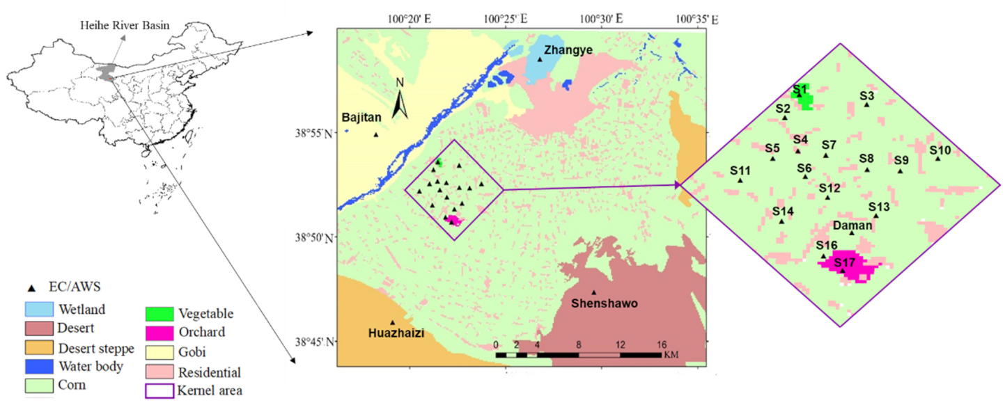
The study area is located in a desert-oasis area in the middle reaches of the Heihe River Basin (HRB) in northwestern China, as shown in Figure 1. The area has a dry continental climate with an average annual air temperature of 8.5 °C (the temperature of 21.1 °C during June to August, the temperature of −6.8 °C during December to February) and mean annual precipitation of 100–250 mm (with a large portion concentrated in summer) during the period of 2012–2018. The altitude in this area ranges between 1360 and 2400 m, and the annual potential evaporation of the study area varies between 1200 mm and 1800 mm. The land cover is complex in the area, with the central part covered by croplands, wetlands and residential areas, and the marginal area covered by the Gobi, desert steppe and sandy deserts.

The Heihe integrated observatory network was established in the study area in 2012 [40,41], and it includes short-term intensive observations and long-term regular observations. The intensive observations were conducted at 21 sites during the Multi-Scale Observation Experiment on Evapotranspiration over Heterogeneous Land Surfaces (HiWATER-MUSOEXE), and long-term observations were conducted continuously at 5 sites which consist the hydro-meteorological observation network (shown in Figure 1).

2.2. Field Measurements

The Heihe integrated observatory network, which is referred to as the Heihe Watershed Allied Telemetry Experimental Research (HiWATER, website: http://hiwater.westgis.ac.cn/, accessed on 22 February 2020), is consisted of two nested test matrices, i.e., one large experimental area (30 × 30 km) and one kernel experimental area (5.5 × 5.5 km), as shown in Figure 1. In this study, the intensive observations from 21 eddy-covariance (EC)/automatic weather stations (AWS) (S1–S17, Daman, Wetland, Huazhaizi, Shenshawo, Bajitan) in the growing season (from May 2012 to September 2012) and the long-term continuous observations from 5 stations (Daman, Wetland, Huazhaizi, Shenshawo, Bajitan) in growing and non-growing seasons (from May 2012 to December 2018) were applied (

Table 1. Information about the stations in the middle reaches of HRB.

Site	Elevation (m)	Land Cover	Time Period (Year/Month/Day)	Long-Term Observations	Underlying Surface
S1	1552.8	vegetable	2012/6/10–2012/9/17	without	vegetation
S2	1559.1	corn	2012/5/3–2012/9/21	without	vegetation
S3	1543.1	corn	2012/6/3–2012/9/18	without	vegetation
S4	1561.9	residential	2012/5/10–2012/9/17	without	——
S5	1567.7	corn	2012/6/4–2012/9/18	without	vegetation
S6	1563.0	corn	2012/5/9–2012/9/21	without	vegetation
S7	1556.4	corn	2012/5/28–2012/9/18	without	vegetation
S8	1550.1	corn	2012/5/14–2012/9/21	without	vegetation
S9	1543.3	corn	2012/6/4–2012/9/17	without	vegetation
S10	1534.7	corn	2012/6/1–2012/9/17	without	vegetation
S11	1575.7	corn	2012/6/2–2012/9/18	without	vegetation
S12	1559.3	corn	2012/5/10–2012/9/21	without	vegetation
S13	1550.7	corn	2012/5/6–2012/9/20	without	vegetation
S14	1570.2	corn	2012/5/6–2012/9/21	without	vegetation
S16	1564.3	corn	2012/6/1–2012/9/17	without	vegetation
S17	1559.6	orchard	2012/5/12–2012/9/17	without	vegetation
Daman	1556.1	corn	2012/5/10–2018/12/31	with	vegetation
Shenshawo	1594.0	desert	2012/6/1–2018/12/31	with	non-vegetation
Huazhaizi	1731.0	desert steppe	2012/6/2–2018/12/31	with	non-vegetation
Bajitan	1562.0	Gobi desert	2012/5/13–2018/12/31	with	non-vegetation
Zhangye	1460.0	wetland	2012/6/25–2018/12/31	with	vegetation

Note: Without represents the observation experiment of the site belonging to intensive observational experiments (HiWATER-MUSOEXE). With represents the observation experiment of the site belonging to intensive observational experiments and long-term observational experiments. Vegetation represents the underlying surface of the site belonging to vegetable, orchard, wetland, or corn. Non-vegetation represents the underlying surface of the site belonging to Gobi, desert steppe, or desert. —— represents the underlying surface of the site not belonging to vegetation or non-vegetation underlying surfaces.

). The 21 AWS/EC stations were located in eight types of land covers (i.e., vegetable, orchard, wetland, corn, residential, desert, desert steppe, Gobi). S1, S4, and S17 are located in vegetable fields, residential areas and orchards, respectively. The land covers of Shenshawo, Huazhaizi, Bajitan, and Zhangye are Gobi, desert steppe, desert, and wetland, respectively. The remaining sites (Daman, S2, S3, S5–16) are located in the cornfield.

Several atmospheric observation data were used in this study, including air pressure, air temperature (T_a), relative humidity (RH), precipitation, soil temperature, soil moisture, upward and downward longwave radiation, upward and downward shortwave radiation, net radiation (Rn), soil heat flux from heat-plates. These variables were measured every 10 min. In order to obtain gridded spatial data of 30 m by 30 m resolution, T_a, RH, and air pressure (from meteorological station) were interpolated through the Inverse Distance Weighted (IDW) method [42]. Soil heat flux (G) was calculated by the Plate Cal method [43], which required the heat-plates flux and the change in heat storage. Soil temperatures (depth of 2 cm and 4 cm), soil moisture (depth of 2 cm and 4 cm), and the porosity were used for calculating the change of heat storage. Due to the lack of soil texture data in Zhangye, Huazhaizi, and S4 stations, the change of heat storage was not calculated in these stations.

The originally measured latent heat flux data were processed by Eddypro software with an interval of 30 min. The data processing included the elimination of outlier, lay time correction, frequency response correction, ultrasonic virtual temperature correction, coordinate rotation, and density fluctuation correction. All the originally measured latent heat flux data have been dealt with Bowen Ratio-Energy Balance (BREB) method [44]. Note that both the latent heat flux data and meteorological data used in present study are observed at 12 AM so as to match the satellite overpassing time.

2.3. Satellite Data

Eight ASTER and forty LANDSAT-8 OLI images without cloud contamination were used (

Table 2. Nearly cloud-free Aster and LANDSAT scene imagery used in this study.

Satellite	Year	Month/Day
Aster	2012	2012/6/15 2012/6/24 2012/7/10 2012/8/2 2012/8/11 2012/8/18 2012/8/27 2012/9/3
LANDSAT	2013	2013/4/16 2013/7/21 2013/10/9 2013/11/10 2013/12/12 2013/12/28
	2014	2014/1/13 2014/2/14 2014/3/2 2014/3/18 2014/7/24 2014/8/9 2014/9/26
	2015	2015/4/22 2015/8/28 2015/9/13 2015/9/29 2015/10/15 2015/12/2
	2016	2016/3/7 2016/4/24 2016/6/27 2016/7/29 2016/9/15 2016/10/1 2016/10/17 2016/11/2 2016/12/4
	2017	2017/1/5 2017/3/26 2017/7/16 2017/11/5 2017/11/21 2017/12/7
	2018	2018/1/8 2018/2/25 2018/9/21 2018/10/7 2018/10/23 2018/11/24

). The overpassing time of ASTER and LANDSAT-8 OLI are between 12:10 and 12:20 (local time) and between 11:55 and 12:00 (local time), respectively. The spatial resolutions of ASTER L1B product and LANDSAT-8 OLI product (level 1 and level 2) are 90 m and 30 m, respectively. The LANDSAT images were obtained along path 133 and row 33, and the ASTER and LANDSAT data were downloaded from the United States Geological Survey (USGS) Earth Resources Observation and Science Center (website: http://glovis.usgs.gov/, accessed on 2 September 2020).

For LANDSAT8 satellite, we calculated Normalized Difference Vegetation Index (NDVI) with band 4 and band 5. Albedo (α) was computed using the algorithm of Liang [45]. Land surface emissivity (ε) was calculated with the algorithm of Sobrino [46]. EVI was calculated with the algorithm of Liu [47]. T_L was calculated using a single-channel (TIRS10) algorithm (JM-SC) [48]. The atmospheric water vapor content (the key parameter in JM-SC) was obtained through the NASA website (https://atmcorr.gsfc.nasa.gov/, accessed on 11 September 2020).

For the Aster satellite, we calculated NDVI with band 2 and band 3. EVI was calculated with the two-band method proposed by Jiang [49]. T_L and ε were estimated using the temperature–emissivity separation algorithm [50]. Albedo (α) was computed using the algorithm of Liang [45].

3. Methods

3.1. WAPT Framework

The Wind-Avoiding Priestley-Taylor algorithm (WAPT) estimates evapotranspiration based on the Priestley-Taylor formula given by [33]:

$$\mathrm{LE}=\Phi \left(\frac{\Delta }{\Delta +\gamma }\right)\left(Rn-G\right)$$

(1)

where LE is the latent heat flux (W/m²); Rn is the surface net radiation (W/m²), calculated with Allen’s method [10]; G is the soil heat flux (W/m²), calculated as a fraction of Rn with Bastiaanssen’s method [51]; γ is the psychrometric constant (kPa/°C); Δ is the slope of saturated vapor pressure versus air temperature (kPa/°C); Φ is the Priestley and Taylor coefficient, which is primarily regulated by the available soil water. Note that the Φ varies from 0 to 1.26, indicating the variation of the actual LE according to the water content of the underlying surface. In this paper, we employed a wind-avoiding trapezoidal space (Figure 2) to simulate the Φ value for any pixel with a given f_c value based on a two-stage linear interpolation method as the following equation [52].

$$\Phi =\frac{\left(T_{L,max}-T_L\right)}{\left(T_{L,max}-T_{L,min}\right)}({\Phi }_{max}-{\Phi }_{min})+{\Phi }_{min}$$

(2)

T_L,max and T_L,min are the maximum and minimum land surface temperatures on the dry and wet edges with the fractional vegetation cover (fc), respectively. Φ_max was set to be 1.26 at the wet edge [13,33]. Φ at point D was set to 0, and Φ at point B was set to 0.1, as the epidermal cuticle transpiration still exists under extreme drought conditions [52,53]. Φ_min can be linearly interpolated between Φ value at point B and D.

3.2. Calculating the Pixel-by-Pixel Φ Value

Wang et al. proposed a robust method to calculate the physically extreme T_L based on energy balance and radiation budget [30,54].

$$T_{L,A}=\frac{\left[r_{ac,A}{R}_{nc,A}/\rho C_P\right]\mathsf{\gamma }\left(1+r_{cm }/r_{ac,A}\right)-\mathrm{VPD}}{\Delta +\mathsf{\gamma }\left(1+r_{cm }/r_{ac,A}\right)}+T_a$$

(3)

$$T_{L,B}=\frac{\left[r_{ac,B}{R}_{nc,B}/\rho C_P\right]\mathsf{\gamma }\left(1+r_{cx }/r_{ac,B}\right)-\mathrm{VPD}}{\Delta +\mathsf{\gamma }\left(1+r_{cx }/r_{ac,B}\right)}+T_a$$

(4)

$$T_{L,C}=\frac{\left[r_{as,C}{R}_{ns,C}\left(1-G_{f,C}\right)/\rho C_P\right]\mathsf{\gamma }-\mathrm{VPD}}{\Delta +\mathsf{\gamma }}+T_a$$

(5)

$$T_{L,D}=r_{as,D}{R}_{ns,D}\left(1-G_{f,D}\right)/\rho C_P+T_a$$

(6)

where subscripts c and s represent the vegetation and soil components hereafter, respectively; subscripts A, B, C, and D represent the values at the four vertices plotted in Figure 2; G_f denotes the ratios of G to R_n; $G_{f,C}$ and $G_{f,D}$ were set to 0.25 and 0.3, respectively; r_cm and r_cx were the minimum and maximum canopy resistances (set to 12.5 s/m and 625 s/m, respectively); r_ac,A, r_ac,B, r_as,C, and r_as,D are the aerodynamic resistances (s/m) at points A, B, C and D, respectively; Δ is the slope of saturated vapor pressure to air temperature (kPa/°C); γ is the psychrometric constant (kPa/°C); VPD is the vapor pressure deficit of the air (kPa); $\rho$ is the air density (kg/m³);$C_P$ is the air specific heat at constant pressure (1004 J/K/kg).

Here, we further modified the calculation of the extreme temperatures to u-avoiding by employing an assumption of no turbulent heat exchange occurring in the vertical direction at the well-watered edge under given meteorological conditions, i.e., the neutral atmospheric conditions of well-watered edge on the basis of the Monin–Obukhov Similarity theory [55]. We can deduce that T_L,A = T_L,C = T_a from the assumption. Then we can calculate the r_ac,B, and r_as,D from neutral atmospheric conditions (i.e., r_ac0 and r_as0) according to Equations (7) and (8) without employing u as input when the T_L,A and T_L,C are known. In practice, we employed the averaged T_a of well-watered landscapes as T_L,A and T_L,C, r_ac,A (or r_as,C) was estimated by r_ac0 (or r_as0) with u independent function f(φ_mc, φ_hc) (or f(φ_ms, φ_hs)).

$$\left\{\begin{array}{c}{r}_{ac,B}=r_{ac0}\times f\left({\phi }_{mc,B},{\phi }_{hc,B}\right)\\ f\left({\phi }_{mc,B},{\phi }_{hc,B}\right)=\left(1-\frac{{\phi }_{mc,B}}{\frac{z-d}{z_{omc,B}}}\right)\left(1-\frac{{\phi }_{hc,B}}{\frac{z-d}{z_{ohc,B}}}\right)\end{array}\right.$$

(7)

$$\left\{\begin{array}{c}{r}_{as,D}=r_{as0}\times f\left({\phi }_{ms,D},{\phi }_{hs,D}\right)\\ f\left({\phi }_{ms,D},{\phi }_{hs,D}\right)=\left(1-\frac{{\phi }_{ms,D}}{\frac{z-d}{z_{oms,D}}}\right)\left(1-\frac{{\phi }_{hs,D}}{\frac{z-d}{z_{ohs,D}}}\right)\end{array}\right.$$

(8)

where φ_hc,B and φ_hs,D are the stability functions for heat at point B and D, it was calculated with Paulson’s method [56], respectively; φ_mc,B and φ_ms,D are the stability functions for momentum at point B and D, it was calculated with Webb’s method [57], respectively; z is meteorological observation height (set to 2 m); d is the zero-displacement height (m) (equal to 2/3 h), and h is the vegetation height (m); z_omc,B and z_oms,D are the roughness length for momentum transfer at point B and D, z_omc,B is set to 1/8 h and z_oms,D is set to 0.005 m [10]; z_ohc,B and z_ohs,D are the roughness length for heat transfer at point B and D.

The procedure for calculating T_L,B and T_L,D on a pixel basis is divided into six major steps:

(1) calculate the initial r_ac,B and r_as,D by assuming f(φ_mc,B, φ_hc,B) = 0 and f(φ_ms,D, φ_hs,D) = 0, i.e., the r_ac0 and r_as0 by means of Equations (9) and (10), respectively.

$$r_{ac0}=\frac{\mathrm{VPD}\rho C_P}{\mathsf{\gamma }{R}_{nc,A}}-r_{cm }$$

(9)

$$r_{as0}=\frac{\mathrm{VPD}\rho C_P}{\mathsf{\gamma }{R}_{ns,C}}$$

(10)

where R_nc,A and R_ns,C can be calculated by:

$$R_{nc,A}=\left(1-{\alpha }_{c,A}\right)R_d+\epsilon {\epsilon }_a\sigma T_a^4-\epsilon \sigma T_{c,A}^4$$

(11)

$$R_{ns,C}=\left(1-{\alpha }_{s,C}\right)R_d+\epsilon {\epsilon }_a\sigma T_a^4-\epsilon \sigma T_{s,C}^4$$

(12)

where α_c,A and α_s,C represent albedos (dimensionless) of vegetation and bare soil, respectively; α_c,A is fixed as 0.2, as the corn area makes more than half of the total study area and the albedo of corn is 0.2 [58]; α_s,C = (α − α_c,A fc)/(1 − fc); R_d is the downward shortwave radiation (W/m²), calculated with Allen’s method [10]; ε is the land surface emissivity (dimensionless) [46]; ε_a is the atmospheric emissivity (dimensionless) and is calculated by the method from Brutsaert [59]; and σ is the Boltzmann constant.

(2) calculate sensible heat flux H_c,B (=0.9R_nc,B) and H_s,D (=R_ns,D(1 − G_f,D));

(3) calculate Monin-Obukhov length L_c,B and L_s,D. L_c,B and L_s,D define the stability conditions of the atmosphere for vegetation and bare soil, respectively, i.e., when L_c,B < 0, the atmospheric condition for vegetable is unstable, and when L_c,B > 0, the atmospheric condition for vegetable is stable. L_c,B and L_s,D are given by Choudhury’s method [60] as:

$$L_{c,B}=\frac{-\rho C_P{U}_{c,B}^{\ast }{}^3{T}_a}{\mathrm{kg}{H}_{c,B}}$$

(13)

$$L_{s,D}=\frac{-\rho C_P{U}_{s,D}^{\ast }{}^3{T}_a}{\mathrm{kg}{H}_{s,D}}$$

(14)

where $\mathrm{g}$ = 9.8 m/s²; $U_{c,B}^{\ast }$ and $U_{s,D}^{\ast }$ are the friction wind speed of the canopy surface and soil surface, which can be calculated by:

$$U_{c,B}^{\ast }=\frac{H_{c,B}}{\rho C_p\frac{(T_{r,B}-T_a)k}{ln\left(\frac{z-d}{z_{ohc,B}}\right)-{\phi }_{hc,B}\left(\frac{z-d}{L_{c,B}}\right)+{\phi }_{hc,B}\left(\frac{z_{ohc,B}}{L_{c,B}}\right)}}$$

(15)

$$U_{s,D}^{\ast }=\frac{H_{s,D}}{\rho C_p\frac{(T_{r,D}-T_a)k}{ln\left(\frac{z-d}{z_{ohs,D}}\right)-{\phi }_{hs,D}\left(\frac{z-d}{L_{s,D}}\right)}}$$

(16)

(4) calculate z_ohc,B (=z_omc,B/exp($k{B}_{c,B}^{-1}$)) and z_ohs,D (=z_oms,D/exp($k{B}_{s,D}^{-1}$)) with $k{B}_{c,B}^{-1}$ and $k{B}_{s,D}^{-1}$ given by the Brutsaert’s method [59] and Massman’s method [61] as:

$$k{B}_{c,B}^{-1}=\frac{\mathrm{k}{C}_d}{4\left(1-e^{-n/2}\right)U_x{C}_t}$$

(17)

$$k{B}_{s,D}^{-1}=2.46{\left(Re\right)}^{1/4}-2$$

(18)

where C_d is the drag coefficient of the foliage elements, set to 0.2 [9]; C_t is the heat transfer coefficient of the leaf, and U_x is a function of non-dimensional drag area density; Re is the roughness Reynolds number (=z_oms,D $U_{s,D}^{\ast }$/v, with v being the kinematic viscosity of the air).

(5) calculate φ_mc,B, φ_ms,D, φ_hc,B and φ_hs,D;

For stable atmospheric conditions at vegetable (L_c,B > 0):

$$\left\{\begin{array}{c}{\phi }_{mc,B}=-5\left(z-z_{omc,B}\right)/L_{mc,B}\\ {\phi }_{hc,B}=-5\left(z-z_{ohc,B}\right)/L_{mc,B}\end{array}\right.$$

(19)

For stable atmospheric conditions at bare soil (L_s,D > 0):

$$\left\{\begin{array}{c}{\phi }_{ms,D}=-5\left(z-z_{oms,D}\right)/L_{ms,D}\\ {\phi }_{hs,D}=-5\left(z-z_{ohs,D}\right)/L_{ms,D}\end{array}\right.$$

(20)

For instable atmospheric conditions at vegetable (L_c,B < 0):

$$\left\{\begin{array}{c}{\phi }_{mc,B}=2\ln \left(\frac{1+x_{c,B}}{2}\right)+\ln \left(\frac{1+x_{c,B}{}^2}{2}\right)-2ta{n}^{-1}\left(x_{c,B}\right)+\pi /2\\ {\phi }_{hc,B}=2\ln \left(\frac{1+x_{c,B}}{2}\right)\end{array}\right.$$

(21)

For instable atmospheric conditions at bare soil (L_s,D < 0):

$$\left\{\begin{array}{c}{\phi }_{ms,D}=2\ln \left(\frac{1+x_{s,D}}{2}\right)+\ln \left(\frac{1+x_{s,D}{}^2}{2}\right)-2ta{n}^{-1}\left(x_{s,D}\right)+\pi /2\\ {\phi }_{hs,D}=2\ln \left(\frac{1+x_{s,D}}{2}\right)\end{array}\right.$$

(22)

where $x_{c,B}={\left[1-\frac{16\left(z-d\right)}{L_{c,B}}\right]}^{1/4}$ and $x_{s,D}={\left[1-\frac{16\left(z-d\right)}{L_{s,D}}\right]}^{1/4}$.

(6) iteratively calculate T_L,B and T_L,D in Equations (4) and (6), R_nc,B and R_ns,D in Equations (11) and (12), H_c,B and H_s,D in step (2), L_c,B and L_s,D in Equations (13) and (14), $U_{c,\mathrm{B}}^{\ast }$ and $U_{s,D}^{\ast }$ in Equations (15) and (16), $k{B}_{c,B}^{-1}$ and $k{B}_{s,D}^{-1}$ in Equations (17) and (18), φ_mc,B, φ_ms,D, φ_hc,B and φ_hs,D in Equations (19)–(22), f(φ_hc,B, φ_mc,B) and f(φ_hs,D, φ_ms,D) in Equations (7) and (8), r_ac,B and r_as,D in Equations (7) and (8), until the r_ac,B and r_as,D are stable, i.e., the difference between two adjacent iterations are less than five percent. Normally, the stability can be satisfied within 10 iterations.

4. Results

4.1. WAPT Model Performance in Four Seasons

The performance of the WAPT model was evaluated with three indicators in this study, i.e., the mean bias error (MBE), root-mean-square error (RMSE), and correlation coefficient (r²) [62]. We first evaluated input variables (Rn and G) during the long-term observation period from 2013 to 2018 using LANDSAT images from 40 dates against the five land covers tower observations. The results are shown in

Table 3. Performance of Rn, G, and LE from the WAPT model during long-term observation periods from 2013 to 2018.

	Rn					G					LE
LUCC	Observed Average (W/m2)	Estimated Average (W/m2)	r2	RMSE (W/m2)	MBE (W/m2)	Observed Average (W/m2)	Estimated Average (W/m2)	r2	RMSE (W/m2)	MBE (W/m2)	Observed Average (W/m2)	Estimated Average (W/M2)	r2	RMSE (W/m2)	MBE (W/m2)
Wetland	435.4	443.8	0.97	31.8	14.0	——	——	——	——	——	277.1	300.7	0.96	49.6	24.2
Corn	371.3	378.6	0.97	33.0	15.7	41.3	42.1	0.27	31.6	15.8	196.1	236.9	0.95	49.8	7.0
Desert steppe	359.2	332.4	0.96	33.5	−25.7	56.3	53.6	0.62	27.0	−7.5	57.7	71.4	0.53	31.7	−6.3
Gobi	334.9	318.8	0.99	14.1	−6.6	57.1	51.8	0.87	21.2	−5.6	65.8	84.3	0.76	43.8	22.8
Desert	345.6	355.9	0.97	27.2	14.2	58.3	58.0	0.89	20.4	−0.5	49.1	66.0	0.77	53.9	41.7
Overall	380.1	365.5	0.96	30.8	3.4	51.2	51.7	0.54	26.7	1.3	150.6	153.8	0.95	46.0	14.0

and Figure 3.

The Rn calculated with WAPT obtained reliable overall accuracy, and it was consistent with the observation (r² of 0.96, Figure 3 and Table 3). The overall RMSE and MBE were 30.8 W/m² and 3.4 W/m², respectively. Simultaneously, its performance varied with landscapes where the Rn was overestimated at wetland, corn, and desert sites (MBE of 14.0 W/m², 15.7 W/m², and 14.2 W/m², respectively). Compared with others, Rn estimation at desert steppe had a larger error with MBE of –25.7 W/m² and RMSE of 33.5 W/m² (Table 3).

There was a relatively large difference between estimated G and observed values (Figure 3). Due to lack of soil porosity measurement, the accuracy of estimated G was only evaluated at sites with corn, desert, desert steppe, and Gobi. The accuracy of G had an overall MBE of 1.3 W/m², RMSE of 26.7 W/m², and r² of 0.54 (Table 3).

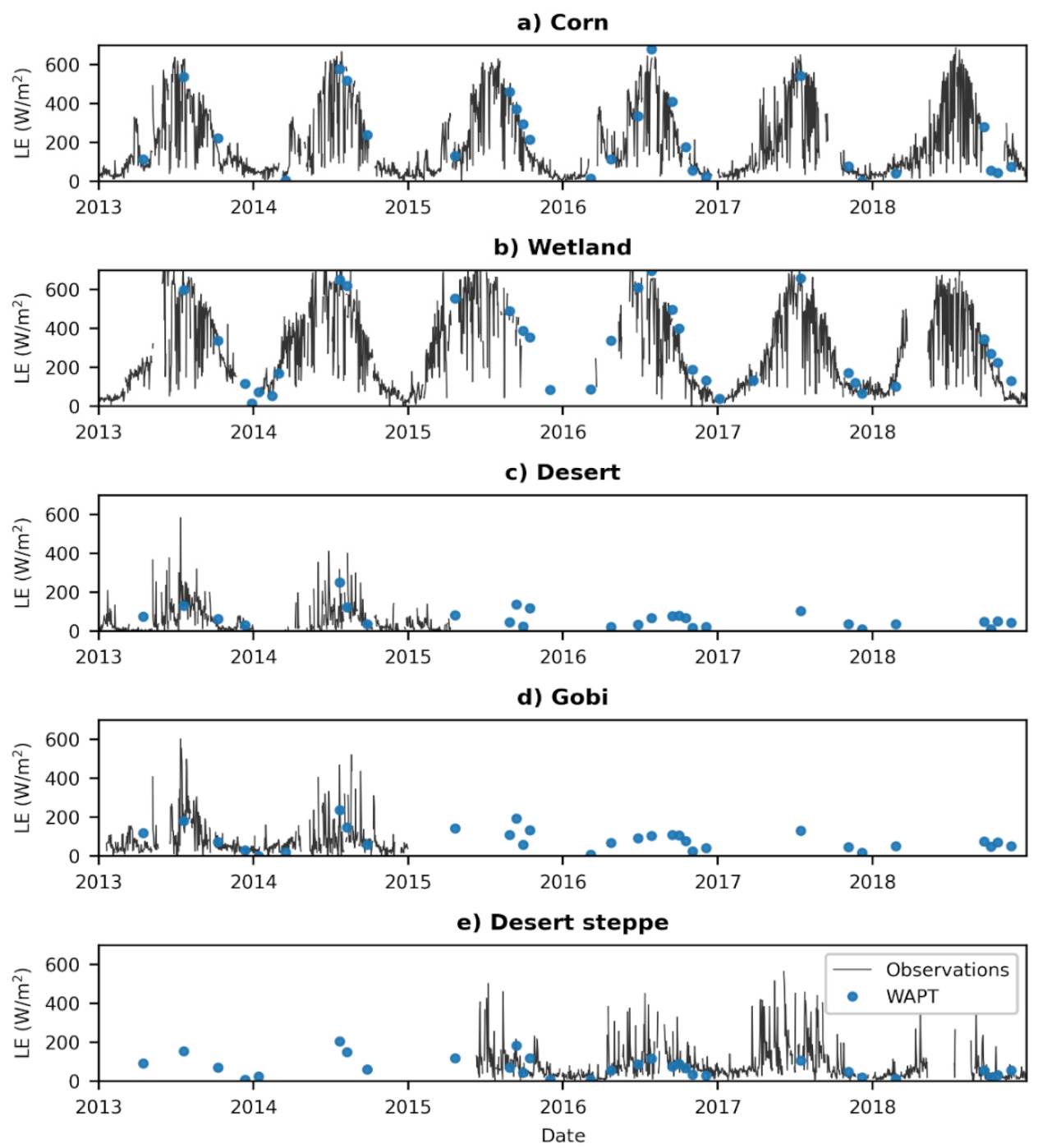
The LE estimates with WAPT model have an overall accuracy with r² of 0.95, RMSE of 46.0 W/m², and MBE of 14.0 W/m² during the long-term observation period. The accuracy presented significant seasonal variation. It had the highest precision in summer (from June to August) and the lowest precision in winter (from December to February). In summer, the WAPT model had r² of 0.96 and RMSE of 45.9 W/m² (

Table 4. Statistics of the modeling LE accuracies in four seasons during 2013–2018, with summer from June to August, autumn from September to November, winter from December to February, and spring from March to May.

Model	Precision Index	Winter	Spring	Summer	Autumn
WAPT	r2	0.36	0.50	0.96	0.91
	MBE	−20.2	16.9	9.7	29.4
	RMSE	37.9	44.2	45.9	49.5

). The WAPT model had underestimated LE values (MBE of −20.2 W/m²) in winter (Figure 4 and Table 4). The WAPT model overestimated the LE in autumn and spring, with MBE of 29.4 and 16.9 W/m², respectively (Figure 4 and Table 4), and had similar RMSE values in autumn and spring, with 49.5 and 44.2 W/m², respectively.

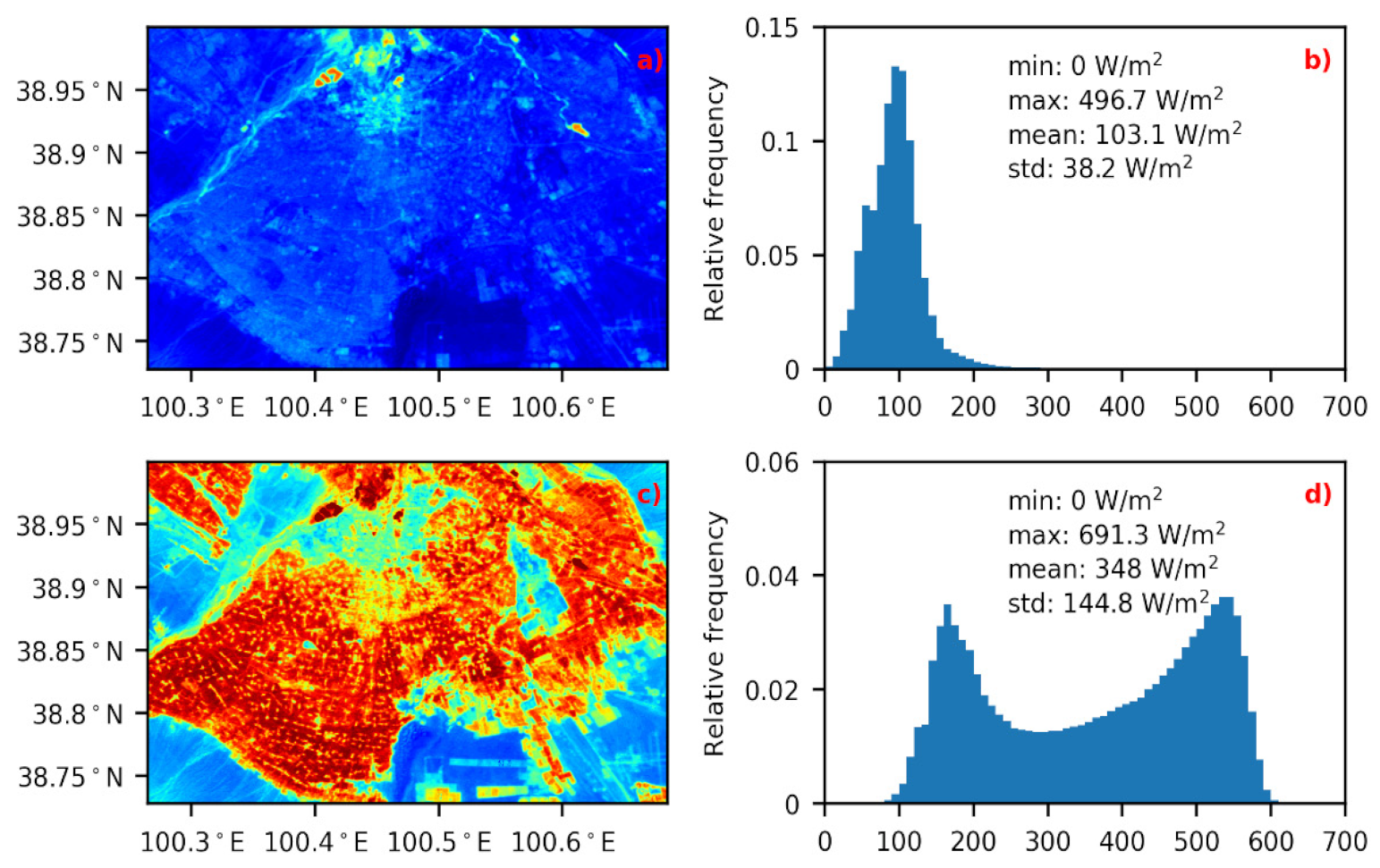
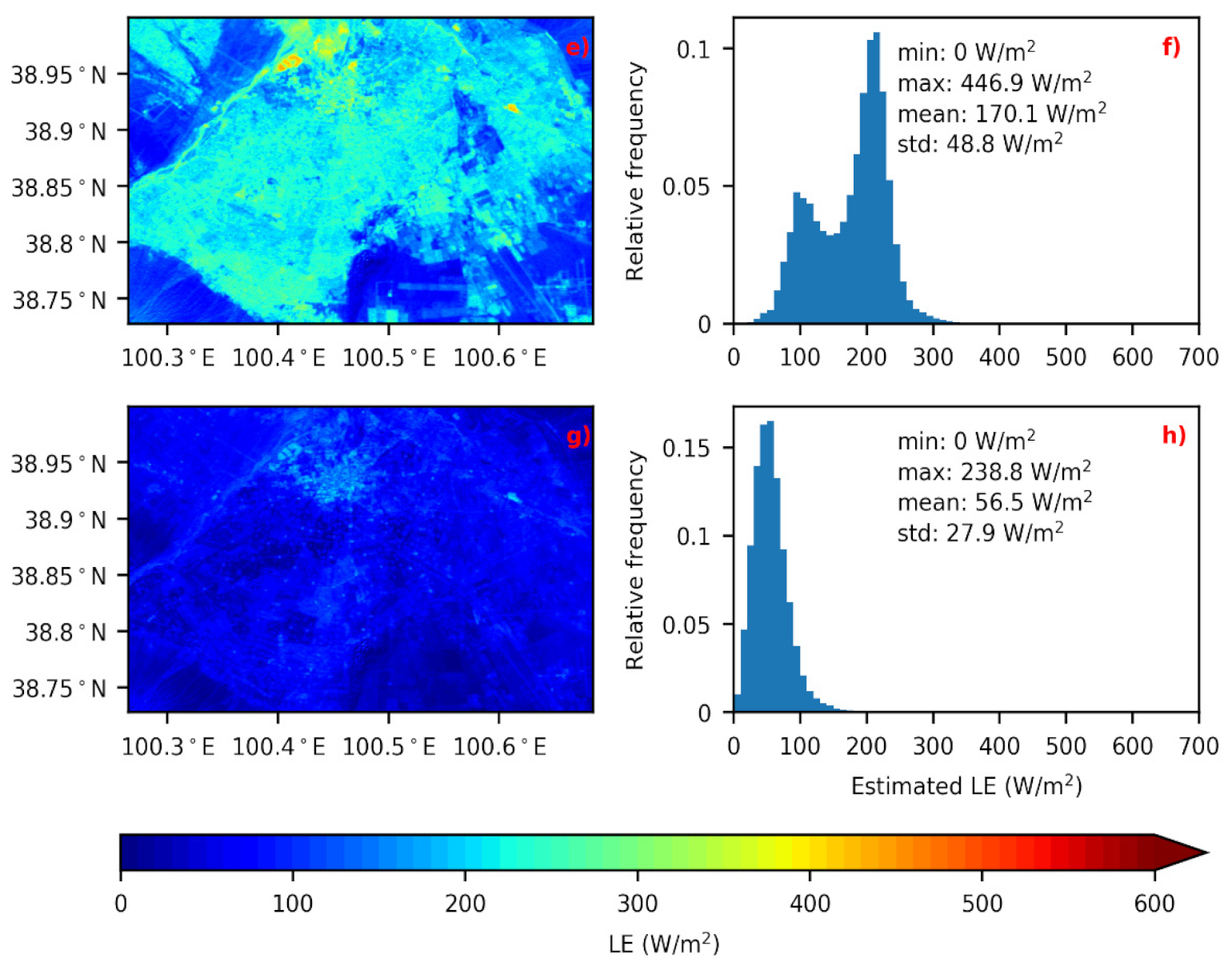
Figure 5 shows the spatial distribution of LE estimates with the WAPT model and their relative frequency distributions in four seasons (averaging over the period 2013–2018). The LE values in four seasons varied greatly. All the underlying surfaces had the highest LE value in summer and the lowest LE value in winter, but the seasonal difference in LE value was larger in vegetated underlying surfaces (e.g., cropland) than non-vegetable underlying surfaces (e.g., desert, desert steppe).

In summer, although the precipitation was sparse, irrigation water was relatively abundant for the cropland during the growing season. Therefore, the cropland (e.g., corn land cover type) had a high LE value ranging from 400 to 500 W/m². For the desert and Gobi, LE was typically around 150 W/m². The relative frequency of LE estimates in the WAPT model explicitly showed the spatial mean value of 348.0 W/m². With the crop harvested, the LE in cropland sharply declined nearly 200 W/m². The LE value in the arid underlying surface, such as desert, was approximately 100 W/m² (Figure 5e,f). Vegetation and non-vegetation underlying surfaces are difficult to be distinguished in the spatial map of spring and winter (Figure 5a,g). The mean spatial LE value was 103.1 W/m² in spring (Figure 5a,b). The mean spatial LE value was much lower in winter than that in spring (56.5 versus 103.1 W/m²), as the temperature rises, and the snow stored in the previous winter melts in spring (more available water for LE consumption) [6].

The LE values on all underlying surfaces had a seasonal variation due to the seasonal change in radiation and different air temperature. It is worth noting that the difference between summer and winter LE values in farmland was larger (more than 400 W/m²) than the arid underlying surface (less than 200 W/m²), which can be attributed to the water supply difference between vegetation and non-vegetation underlying surfaces, such as soil moisture has a higher value in farmland than the desert station in the growing season due to irrigation [63].

4.2. WAPT Model Performance over High Heterogeneous Land Surfaces

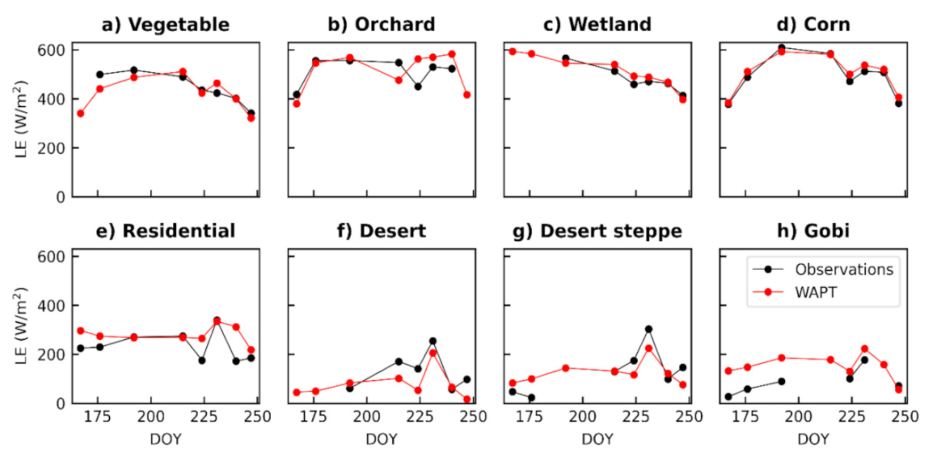
The LE from WAPT was further compared with HiWATER-MUSOEXE-12 observations from May to September in 2012. The comparison between the estimates of LE and flux tower measurements is shown in

Table 5. Statistics of the modeling LE accuracies during months 6–9 in 2012.

LUCC	Observed Average (W/m2)	WAPT
		Estimated Average (W/m2)	r2	RMSE (W/m2)	MBE (W/m2)
Residential	233.8	250.8	0.18	53.0	17.0
Desert	106.1	94.8	0.56	53.4	−6.9
Desert steppe	131.8	122.5	0.56	61.6	−2.8
Gobi	87.3	127.3	0.39	54.9	33.1
Vegetable	443.8	391.6	0.84	51.7	−43.9
Orchard	511.3	479.7	0.48	56.1	8.7
Wetland	480.6	504.9	0.75	25.1	0.9
Corn	489.4	479.8	0.73	48.3	−12.2
Overall	418.5	413.8	0.90	49.6	−9.4

. The accuracy of LE estimates with the WAPT model varied greatly for different underlying surfaces. Overall, the WAPT model behaved better for the land surface with vegetation coverage (i.e., wetland, corn, vegetable, and orchard) than for non-vegetation surfaces (i.e., desert, desert steppe and Gobi).

For sites of vegetation underlying surfaces, the WAPT model agreed well with corresponding ground observations (Table 5 and Figure 6). The RMSE of WAPT model was 25.1 and 48.3 W/m² for wetland and corn sites, respectively. However, the WAPT had a slightly worse precision for vegetable and orchard sites than for wetland and corn sites, with the higher RMSE (51.7 and 56.1 W/m²) value. It may be attributed to a lower land surface temperature precision for vegetable and orchard sites. Furthermore, the WAPT model captured the trends of LE variations for wetland, corn, and vegetable sites through 8 days in 2012 during the whole growing season (Figure 6a,c,d).

For non-vegetation sites (desert, desert steppe, and Gobi), the WAPT model had a lower precision than for vegetation sites, with higher RMSE (53.4, 61.6, and 54.9 W/m² for desert, desert steppe, and Gobi, respectively) and MBE (−26.9, −12.8, and 33.1 W/m² for desert, desert steppe, and Gobi, respectively). Observed LE values for non-vegetation sites (unaffected by human activities, such as irrigations) had a significant fluctuation during months 6–9 in 2012 (Figure 6f–h), as a result of the effective precipitation two days before DOY 231. The proposed WAPT model can simulate the temporal fluctuation of LE for these three non-vegetation sites (desert, desert steppe, and Gobi).

We further compared the accuracy among several remote sensing evapotranspiration models for different underlying surfaces in the literature, and the results are summarized in

Table 6. Comparison of LE (W/m²) estimation accuracies with different models for different surfaces in the midstream of HRB.

References	Model/Method	Images (Dates)	Model Performance (RMSE W/m2)
			Vegetation Underlying (Cropland, Wetland Vegetable, Orchard)	Non-Vegetation (Desert Steppe, Gobi, Desert)	Whole Precision (All Surfaces)
[31]	TD-TSEB n	Landsat (June–September 2012)	cropland: 89.8		89.8
[28]	OSML n	ASTER (July–August 2012)	cropland: 45.0		67.0
[54]	WiTSEB n	ASTER (June–September 2012)	cropland: 56.4 wetland: 76.6 vegetable: 115.1 orchard: 35.6	desert steppe: 118.7 Gobi: 66.7 desert: 95.0	68.6
[64]	RSLE n	MODIS and ASTER (Jun–September 2012)	cropland: 73.6 wetland: 79.8 vegetable: 73.6 orchard: 239.6	Gobi: 68.0 desert: 105.6	144.2
[65]	SEBS u	ASTER (May–September 2012)	cropland: 54.0 b wetland: 72.0 b vegetable: 98.0 b orchard: 25.0 b	desert steppe: 55.0 b Gobi: 58.0 b desert: 39.0 b	64.0
[36]	ATI-PT u	MODIS (Jun–September 2012)	cropland: 51.1 vegetable: 13.9	Gobi: 40.4 desert: 43.4	37.2 m
	SM-PT u		cropland: 42.4 vegetable: 23.6	Gobi: 28.5 desert: 18.2	28.2 m
	VPD-PT u		cropland: 44.5 vegetable: 19.1	Gobi: 38.2 desert: 43.1	36.2 m
[66]	Shuttleworth–Wallace + Bayesian u		cropland: 80.7		80.7

Note: Superscripts u and n represent the u-dependent and u-independent models, respectively. Superscript b indicated that the observed LE is corrected via the Bowen ratio method. Superscript m indicates that the RMSE value presented here is a mean value for different underlying surfaces.

. The comparison shows that the WAPT model provide acceptable accuracy compared with other models. The RMSE of LE for crop and wetland underlying surfaces with different methods was between 42.4 and 89.8 W/m², and the median was 64.2 W/m². Wherein, u-independent models included TD-TSEB [31], OSML [28], WiTSEB [54], and RSLE [64], which provided the RMSE between 45.0 and 89.8 W/m². The WAPT model had a lower RMSE for cropland and wetland (48.3 and 25.1 W/m², respectively). The RMSE of LE for orchard and vegetable surfaces via different methods varied largely between 13.9 and 239.6 W/m²; it may be attributed to the different assumptions in their models. The WAPT model showed a relatively lower RMSE for orchard and vegetable sites than other u-independent models. The RMSE of LE for non-vegetation surfaces with different methods varied largely between 18.2 and 118.7 W/m², with a median of 49.2 W/m². Wherein, WiTSEB [54] and RSLE [64] provided the RMSE varying between 66.7 and 118.7 W/m². The WAPT model had a lower RMSE varying between 53.4 and 61.6 W/m² (for desert, desert steppe, and Gobi).

4.3. Sensitivity Analysis

The inputs of WAPT model include the following parameters: (1) measured meteorological data at the stations: T_a, RH; (2) remote sensing data: T_L, albedo, land surface emissivity, and EVI; (3) momentum rough length of soil (z_oms,D) and vegetation (z_omc,B). Because z_omc,B is set as 1/8 h in this paper, and h is mostly insensitive to LE estimations in trapezoid framework based models (e.g., TTME, HTEM and TMEF), so this paper only investigates parameter z_oms,D. The sensitivity (S) of LE to a parameter (i) is defined as:

$$S_i=\frac{{\mathrm{LE}}_{\pm }-{\mathrm{LE}}_0}{{\mathrm{LE}}_0}\times 100\%$$

(23)

where ${\mathrm{LE}}_0$ is the averaged LE estimated by actual input parameters, ${\mathrm{LE}}_{\pm }$ is the average LE of LANDSAT and ASTER images in the study area estimated by the input parameter i, where ${\mathrm{LE}}_{+}$ or ${\mathrm{LE}}_{-}$ means the LE estimates is increased or decreased with respect to the actual inputs. The perturbations of T_L and T_a are specified as [−4 K, 4 K], with a variation step of 0.5 K. Perturbations of the other variables were specified as [−20%, 20%], with a variation step of 5%.

The WAPT model was the most sensitive to T_a and T_L, which were positively and negatively correlated with LE values, respectively (Figure 7a). A 4 K decrease (increase) in T_a led to a 46.2% decrease (51.2% increase) in LE estimates. A 4 K decrease in T_L resulted in a 40.0% increase in LE estimates, whereas the equal increase (4 K) caused a 34.0% decrease.

RH and z_oms,D were negatively and positively correlated with WAPT LE results, respectively (Figure 7b). The perturbation of LE was nearly 5% when the RH changed by 20%. The perturbation of LE was very small (0.2%) when a 20% change was applied to the z_oms,D in the WAPT model. It suggests that the effect of z_oms,D on the WAPT LE values can be overlooked.

For the WAPT model, the LE value had a negative correlation with the albedo and EVI but had a positive correlation with the land surface emissivity (Figure 7c). A relative change of −20% (20%) perturbation in albedo and EVI caused perturbations of 2.6% (−2.6%) and −3.3% (3.3%) of LE, respectively. The land surface emissivity had a larger influence on LE results, with a −8.3% decrease or 8.7% increase in LE estimates (when the land surface emissivity increased or decreased 20%, respectively).

5. Discussions

5.1. Comparison of WAPT Model and Other u-Independent Models over Seasons

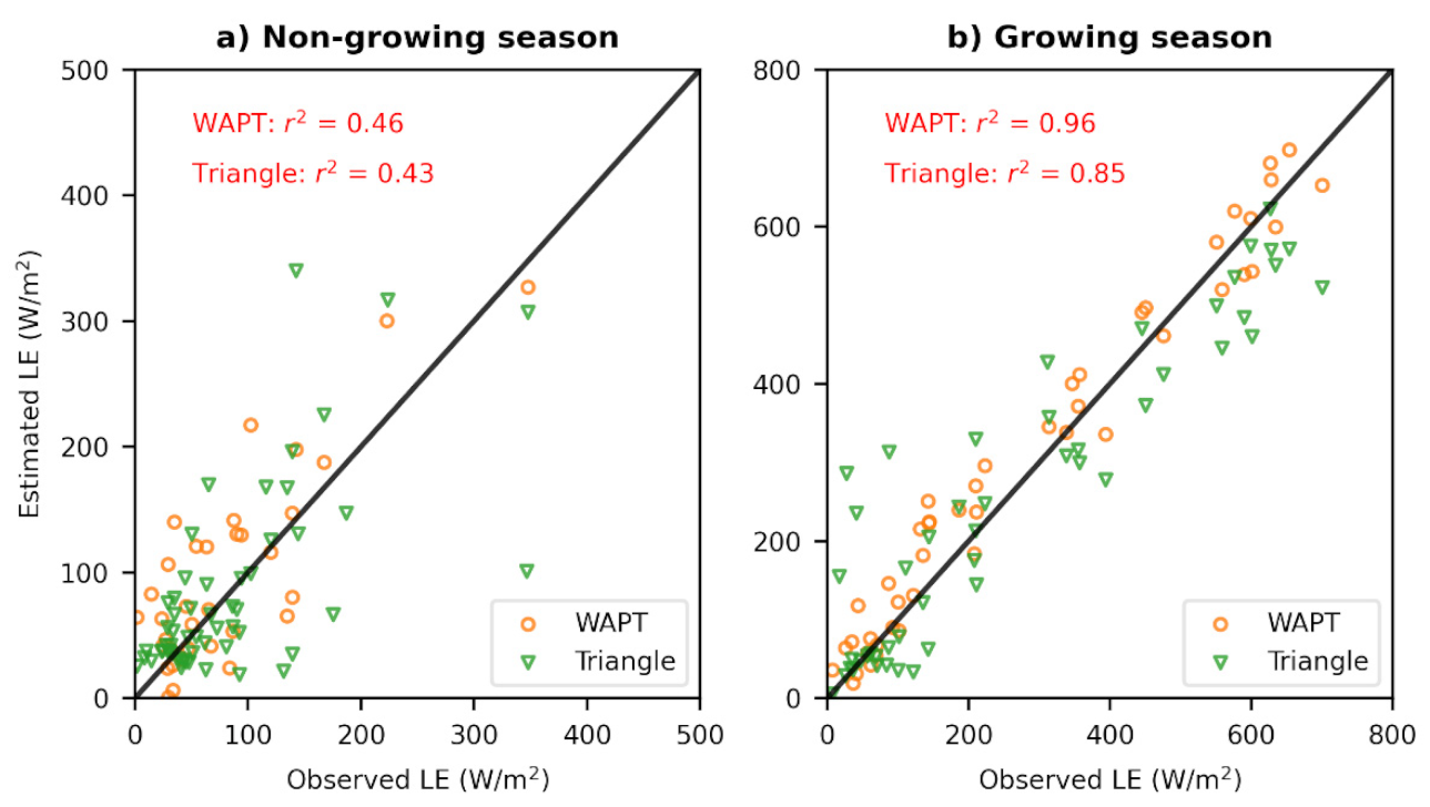
The triangle model [22] is a u-independent model which has been widely used in previous studies [38,67,68,69,70,71]. In this section, the WAPT is compared with the triangle model over growing seasons (May to October) and non-growing seasons (November to April) during 2013–2018.

The WAPT performed well in the growing season but underestimated LE in the non-growing season, while the triangle model had a contrasting performance (overestimated LE in the non-growing season). For the WAPT model, the estimated LE values over the growing season were closer to the observed data in comparison with those in the non-growing season (Figure 8). Similarly, the performance of WAPT model in the growing season was better. Some other studies [72,73] also show that models behave better in the growing season.

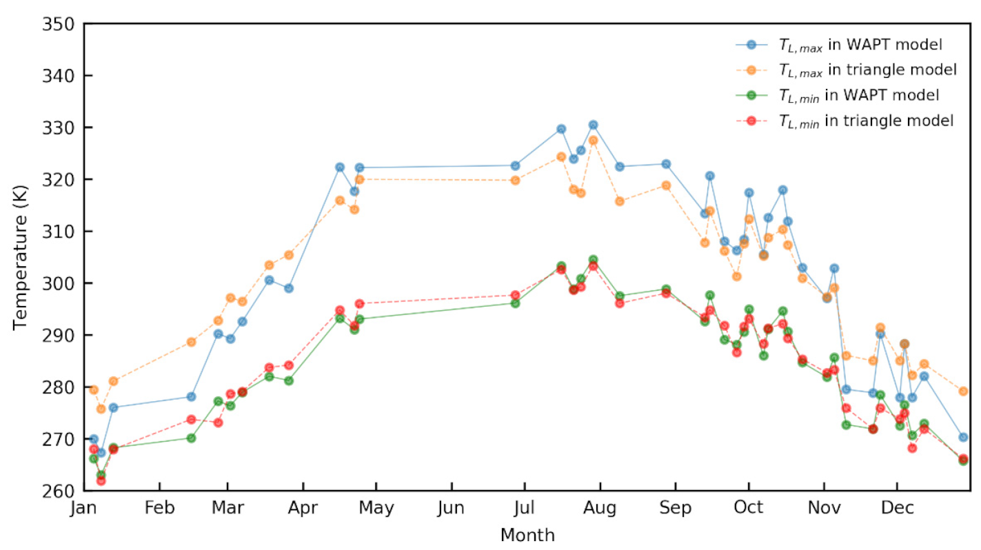
The difference between implementing WAPT and the triangle model was the procedure of constructing the feature space. Therefore, it is necessary to assess the feature space (T_L,max and T_L,min) constructed by two models. The spatial mean results of T_L,max and T_L,min from satellite images in 40 days are presented in Figure 9. Both values of T_L,max and T_L,min from the two models were high in the growing season and low in the non-growing season, but a larger fluctuation was found in T_L,max (ranges from 265 to 340 K) compared with T_L,min (ranges from 260 to 300 K). The T_L,min difference between the two models was smaller than the T_L,max. The T_L,max of WAPT model was larger than the triangle model (4.4 K larger on average in 40 days) in the growing season, but it was smaller than the triangle model (3.7 K lower on average in 40 days) in the non-growing season (Figure 9).

For the triangle model, the T_L,max and T_L,min values are determined empirically based on satellite images [21]. Therefore, the triangle model cannot capture the actual T_L,max and T_L,min values accurately due to dry/wet pixels (dry pixels are located in desert, desert steppe and Gobi landcovers in the image, wet pixels are located in wetland, corn, vegetable, orchard landcovers in the image) ratios and vegetation coverage [3,18]. A small percentage of arid underlying surfaces was in the image while vegetation underlying surfaces occupied a vast majority area in summer (such as dates 27 June, 10 July, 17 July, and 9 August). Thus, the T_L,max may be underestimated due to lacking a sufficient amount of dry pixels from the image. In winter, a small vegetation fraction range was found from the images due to the crop harvest (such as dates 5 January, 10 November, and 2 December). It caused a relatively high T_L,max value estimated from the triangle model.

For the WAPT model, the T_L,max and T_L,min values on the dry and wet edges can be determined on a pixel basis, and it is not affected by the ratio of wet/dry pixels in the image which is required with the triangle method. However, the WAPT model was very sensitive to T_L (Figure 7a). T_L was calculated from the J-M algorithm using LANDSAT-8 satellite data. In this paper, the WAPT model underestimated LE in winter. It can be attributed to the overestimated T_L in winter. This phenomenon was also found in some studies using the J-M algorithm in cold environments (air temperature lower than −5 °C) [74,75,76].

5.2. WAPT Model Performance over Vegetation and Non-Vegetation Surfaces

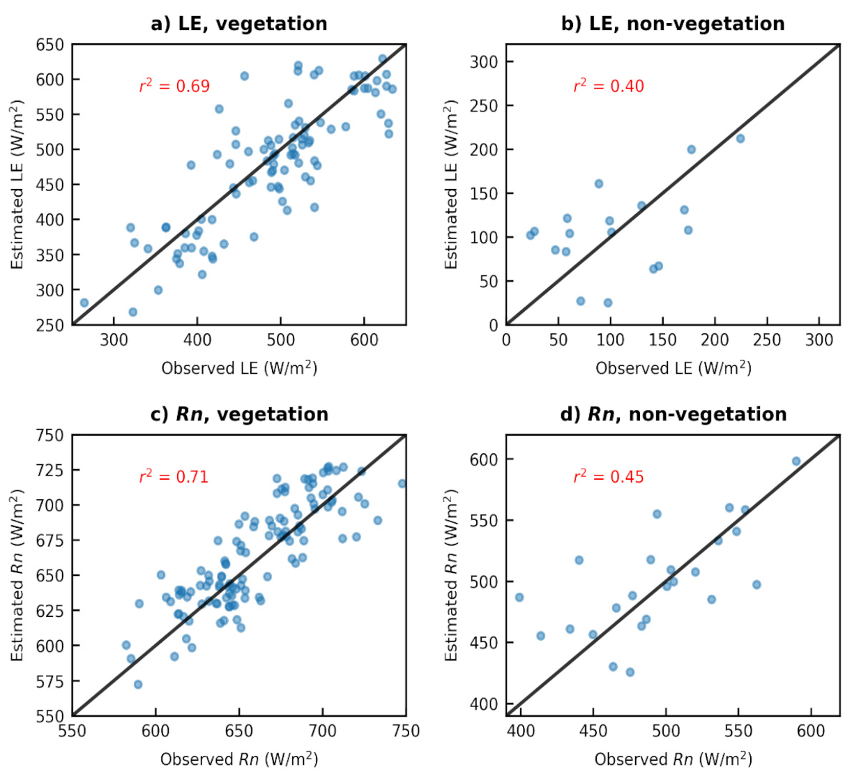
WAPT performed better on vegetation surfaces than non-vegetation surfaces during the growing season in 2012, as shown in Figure 10a,b. This phenomenon is consistent with other u-independent models (e.g., WiTSEB [54], RSLE [64]). The primary reason is the difference in the accuracy of net radiation estimations between vegetation and non-vegetation surfaces (Figure 10c,d). Furthermore, the WAPT LE precision between these two types of underlying surfaces was also affected by setting air temperature as wet edge and using BREB method to verify originally measured latent heat flux data.

The air temperature in different surfaces differed, with the higher T_a in arid underlying surfaces. For the wet area, it is common to use air temperature as the wet edge (T_L,min) [16,17,25]. For the arid surfaces, some researchers pointed out that it is not appropriate to set the air temperature for the wet edge as T_a in arid area, which may overestimate LE value [16,19]. With the higher air temperature in the arid area, the larger wet edge is generated, causing a relatively higher $\Phi$ (and LE value) for the arid area. In this study, air temperature T_a acts as the wet edge in the WAPT model, MBE of the LE with WAPT in the non-vegetation surface was 6.7 W/m², which means a slight overestimation from the WAPT model.

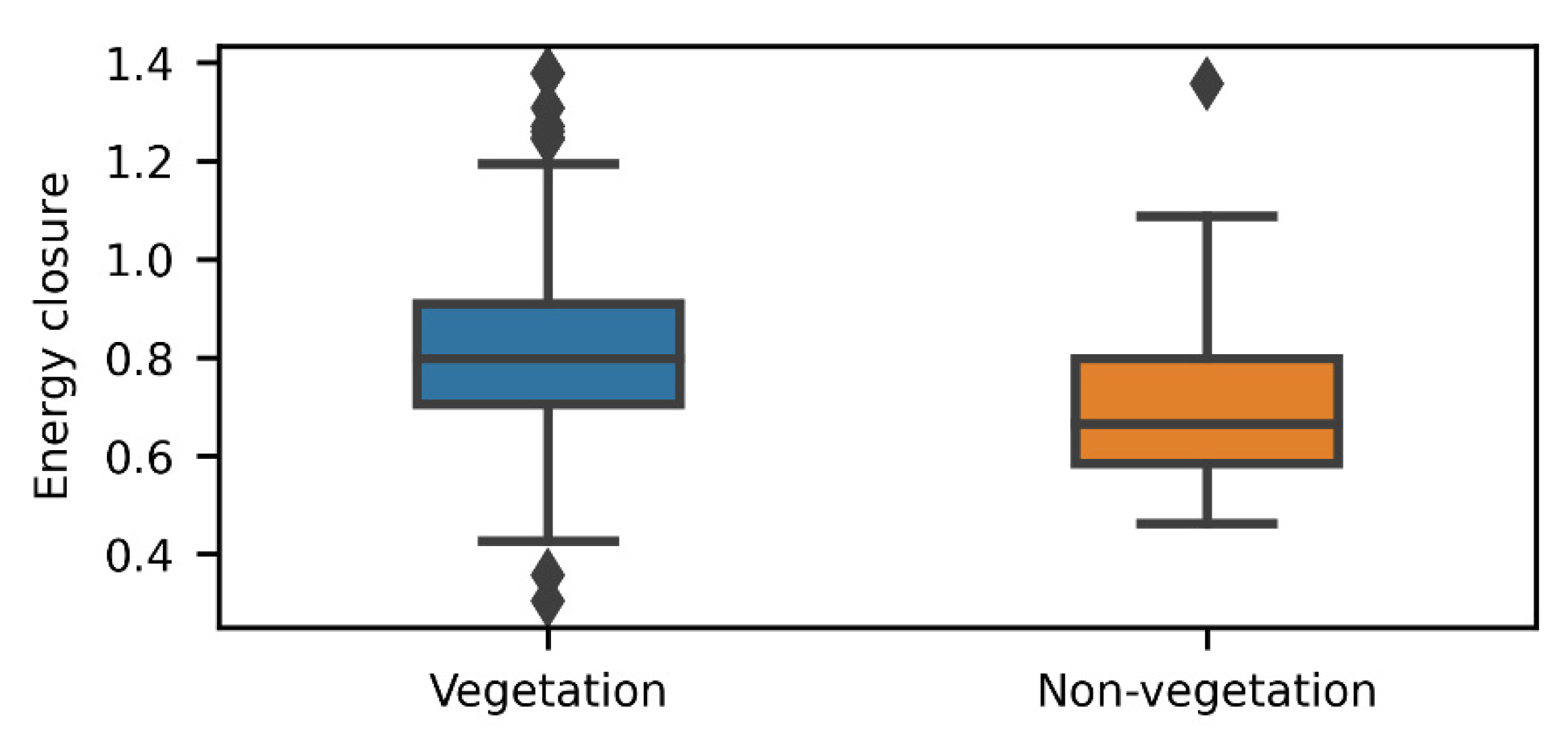
The originally measured data was dealt with BREB method, however, the energy closure was different over vegetation and non-vegetation underlying surfaces, it will involve different uncertainty and error to the observed data that directly compared with WAPT model. In this paper, through the boxplot of energy closure on vegetation and non-vegetation underlying surfaces (Figure 11), we can find that the medians of energy closure in the vegetation and non-vegetation underlying surfaces were 0.8 and 0.67, respectively. The observed data through BREB method in the non-vegetation surface had a higher uncertainty and error. Then, it may be attributed to the lower LE accuracy in the non-vegetation surface for the WAPT model compared with the observed data.

5.3. Advantages and Disadvantages of WAPT Model

There are several merits of the WAPT model. Firstly, information on u is not required in the WAPT model. The data requirement of WAPT can readily be met by involving other routinely observed meteorological variables (T_a, RH, and air pressure) and remotely sensed parameters (T_L, $\epsilon$, NDVI and Albedo). In most one-source and two-source models, e.g., SEBAL [51], SEBS [9], and TSEB [11], u is an indispensable model input. Compared with these models, the WAPT model avoiding u would make it more suitable for the operability of mapping field latent fluxes and real-time. Secondly, the WAPT model adopts theoretical trapezoidal feature space, with its dry/wet edges determined on grid basis theoretically, so the precision of LE estimates is not affected by the satellite image size or cloud contamination.

The WAPT model also has limitations. The region along the middle reaches of the HRB is a composition of oasis and desert ecosystem, where well-irrigated farmlands are strongly affected by heat advection from the surrounding arid area. However, most one-source and two-source models, e.g., SEBAL, TTME, and TMEF, do not consider advection, either the WAPT model. In addition, the LE estimates in the WAPT are sensitive to T_a and T_L, and the errors in either T_a or T_L can reduce the accuracy of LE estimation.

6. Conclusions

To reduce the dependence on wind speed due to its high temporal and spatial variation, a Wind Avoiding Priestley–Taylor (WAPT) algorithm was proposed by employing a u-independent T_L − fc trapezoid space. The WAPT was applied to the arid area in the midstream of HRB during a long-term temporal period (2013–2018). Overall, the performance of WAPT is comparable to other published studies. Temporally, the long-term comparison indicates that the precision of WAPT has a seasonal variation. WAPT had a higher r² value in the growing season (0.96) than in the non-growing season (0.46). Spatially, WAPT had a higher precision in the vegetation surface (r² = 0.69) than the non-vegetation surface (r² = 0.40). The sensitivity analysis suggests that the WAPT model is most sensitive to T_a and T_L but insensitive to other parameters (such as RH, z_oms,D, albedo and EVI).

This study suggests that the WAPT is promising and can be used to estimate regional surface latent flux over heterogeneous surfaces in arid area. In the future work, we will validated the WAPT model in various ecosystems, and some parameters (such as α_c,A) in WAPT model would be calibrated in different physiographic conditions to furtherly improve the model performance.

References

- Miralles, D.G.; Holmes, T.R.H.; De Jeu, R.A.M.; Gash, J.H.; Meesters, A.G.C.A.; Dolman, A.J. Global land-surface evaporation estimated from satellite-based observations. Hydrol. Earth Syst. Sci. 2011, 15, 453–469. [Google Scholar] [CrossRef] [Green Version]
- Mu, Q.; Zhao, M.; Running, S.W. Improvements to a MODIS global terrestrial evapotranspiration algorithm. Remote Sens. Environ. 2011, 115, 1781–1800. [Google Scholar] [CrossRef]
- Wang, K.; Dickinson, R.E. A review of global terrestrial evapotranspiration: Observation, modeling, climatology, and climatic variability. Rev. Geophys. 2012, 50, 1–54. [Google Scholar] [CrossRef]
- Zhang, K.; Kimball, J.S.; Running, S.W. A review of remote sensing based actual evapotranspiration estimation. WIREs Water 2016, 3, 834–853. [Google Scholar] [CrossRef]
- Wang, H.; Li, X.; Xiao, J.; Ma, M. Evapotranspiration components and water use efficiency from desert to alpine ecosystems in drylands. Agric. For. Meteorol. 2021, 298–299, 108283. [Google Scholar] [CrossRef]
- Chen, Y.; Wang, S.; Ren, Z.; Huang, J.; Wang, X.; Liu, S.; Deng, H.; Lin, W. Increased evapotranspiration from land cover changes intensified water crisis in an arid river basin in northwest China. J. Hydrol. 2019, 574, 383–397. [Google Scholar] [CrossRef]
- Kalma, J.D.; McVicar, T.R.; McCabe, M.F. Estimating land surface evaporation: A review of methods using remotely sensed surface temperature data. Surv. Geophys. 2008, 29, 421–469. [Google Scholar] [CrossRef]
- Bastiaanssen, W.G.M.; Pelgrum, H.; Wang, J.; Ma, Y.; Moreno, J.F. A remote sensing surface energy balance algorithm for land (SEBAL) 2. Validation. J. Hydrol. 1998, 212–213, 213–229. [Google Scholar] [CrossRef]
- Su, Z. The Surface Energy Balance System (SEBS) for estimation of turbulent heat fluxes. Hydrol. Earth Syst. Sci. 2002, 6, 85–99. [Google Scholar] [CrossRef]
- Allen, R.G.; Tasumi, M.; Morse, A.; Trezza, R.; Wright, J.L.; Bastiaanssen, W.; Kramber, W.; Lorite, I.; Robison, C.W. Satellite-Based Energy Balance for Mapping Evapotranspiration with Internalized Calibration (METRIC)—Applications. J. Irrig. Drain. Eng. 2007, 133, 395–406. [Google Scholar] [CrossRef]
- Norman, J.M.; Kustas, W.P.; Humes, K.S. Source approach for estimating soil and vegetation energy fluxes in observations of directional radiometric surface temperature. Agric. For. Meteorol. 1995, 77, 263–293. [Google Scholar] [CrossRef]
- Gan, G.; Gao, Y. Estimating time series of land surface energy fluxes using optimized two source energy balance schemes: Model formulation, calibration, and validation. Agric. For. Meteorol. 2015, 208, 62–75. [Google Scholar] [CrossRef]
- Long, D.; Singh, V.P.; Scanlon, B.R. Deriving theoretical boundaries to address scale dependencies of triangle models for evapotranspiration estimation. J. Geophys. Res. Atmos. 2012, 117, D05113. [Google Scholar] [CrossRef]
- Long, D.; Singh, V.P. A modified surface energy balance algorithm for land (M-SEBAL) based on a trapezoidal framework. Water Resour. Res. 2012, 48, W02528. [Google Scholar] [CrossRef]
- Feng, J.; Wang, Z. A satellite-based energy balance algorithm with reference dry and wet limits. Int. J. Remote Sens. 2013, 34, 2925–2946. [Google Scholar] [CrossRef]
- Yang, Y.; Shang, S. A hybrid dual-source scheme and trapezoid framework–based evapotranspiration model (HTEM) using satellite images: Algorithm and model test. J. Geophys. Res. Atmos. 2013, 118, 2284–2300. [Google Scholar] [CrossRef]
- Sun, H. A two-source model for estimating evaporative fraction (TMEF) coupling Priestley-Taylor formula and two-stage trapezoid. Remote Sens. 2016, 8, 248. [Google Scholar] [CrossRef] [Green Version]
- Li, Z.-L.; Tang, R.; Wan, Z.; Bi, Y.; Zhou, C.; Tang, B.; Yan, G.; Zhang, X. A Review of Current Methodologies for Regional Evapotranspiration Estimation from Remotely Sensed Data. Sensors 2009, 9, 3801–3853. [Google Scholar] [CrossRef] [PubMed] [Green Version]
- Petropoulos, G.; Carlson, T.N.; Wooster, M.J.; Islam, S. A review of Ts/VI remote sensing based methods for the retrieval of land surface energy fluxes and soil surface moisture. Prog. Phys. Geogr. 2009, 33, 224–250. [Google Scholar] [CrossRef] [Green Version]
- Kustas, W.P.; Norman, J.M. A two-source approach for estimating turbulent fluxes using multiple angle thermal infrared observations. Water Resour. Res. 1997, 33, 1495–1508. [Google Scholar] [CrossRef]
- Jiang, L.; Islam, S. A methodology for estimation of surface evapotranspiration over large areas using remote sensing observations. Geophys. Res. Lett. 1999, 26, 2773–2776. [Google Scholar] [CrossRef] [Green Version]
- Jiang, L.; Islam, S. Estimation of surface evaporation map over southern Great Plains using remote sensing data. Water Resour. Res. 2001, 37, 329–340. [Google Scholar] [CrossRef] [Green Version]
- Moran, M.S.; Clarke, T.R.; Inoue, Y.; Vidal, A. Estimating crop water deficit using the relation between surface-air temperature and spectral vegetation index. Remote Sens. Environ. 1994, 49, 246–263. [Google Scholar] [CrossRef]
- Wang, W.; Huang, D.; Wang, X.-G.; Liu, Y.-R.; Zhou, F. Estimation of soil moisture using trapezoidal relationship between remotely sensed land surface temperature and vegetation index. Hydrol. Earth Syst. Sci. 2011, 15, 1699–1712. [Google Scholar] [CrossRef] [Green Version]
- Long, D.; Singh, V.P. A Two-source Trapezoid Model for Evapotranspiration (TTME) from satellite imagery. Remote Sens. Environ. 2012, 121, 370–388. [Google Scholar] [CrossRef]
- Yu, B.; Shang, S.; Zhu, W.; Gentine, P.; Cheng, Y. Mapping daily evapotranspiration over a large irrigation district from MODIS data using a novel hybrid dual-source coupling model. Agric. For. Meteorol. 2019, 276–277, 107612. [Google Scholar] [CrossRef]
- Sun, H.; Wang, Y.; Liu, W.; Yuan, S.; Nie, R. Comparison of three theoretical methods for determining dry and wet edges of the LST/FVC space: Revisit of method physics. Remote Sens. 2017, 9, 528. [Google Scholar] [CrossRef] [Green Version]
- Yang, Y.; Qiu, J.; Su, H.; Bai, Q.; Liu, S.; Li, L.; Yu, Y.; Huang, Y. A One-Source Approach for Estimating Land Surface Heat Fluxes Using Remotely Sensed Land Surface Temperature. Remote Sens. 2017, 9, 43. [Google Scholar] [CrossRef] [Green Version]
- Zhao, W.L.; Xiong, Y.J.; Paw U, K.T.; Gentine, P.; Chen, B.; Qiu, G.Y. Uncertainty caused by resistances in evapotranspiration. Hydrol. Earth Syst. Sci. Discuss. 2019, 1–41. [Google Scholar] [CrossRef]
- Wang, X.; Kang, Q.; Chen, X.; Fu, Q.; Wang, P. A Temperature-Domain SEBAL Model Based on a Wind Speed-Independent Theoretical Trapezoidal Space Between Fractional Vegetation Coverage and Land Surface Temperature. IEEE Geosci. Remote Sens. Lett. 2021, 18, 756–760. [Google Scholar] [CrossRef]
- Yao, Y.; Liang, S.; Yu, J.; Chen, J.; Liu, S.; Lin, Y.; Fisher, J.B.; McVicar, T.R.; Cheng, J.; Jia, K.; et al. A simple temperature domain two-source model for estimating agricultural field surface energy fluxes from Landsat images. J. Geophys. Res. Atmos. 2017, 122, 5211–5236. [Google Scholar] [CrossRef]
- Hao, Y.; Baik, J.; Choi, M. Developing a soil water index-based Priestley–Taylor algorithm for estimating evapotranspiration over East Asia and Australia. Agric. For. Meteorol. 2019, 279, 107760. [Google Scholar] [CrossRef]
- Priestley, C.H.B.; Taylor, R.J. On the Assessment of Surface Heat Flux and Evaporation Using Large-Scale Parameters. Mon. Weather Rev. 1972, 100, 81–92. [Google Scholar] [CrossRef]
- Jin, Y.; Randerson, J.T.; Goulden, M.L. Continental-scale net radiation and evapotranspiration estimated using MODIS satellite observations. Remote Sens. Environ. 2011, 115, 2302–2319. [Google Scholar] [CrossRef] [Green Version]
- Fisher, J.B.; Tu, K.P.; Baldocchi, D.D. Global estimates of the land-atmosphere water flux based on monthly AVHRR and ISLSCP-II data, validated at 16 FLUXNET sites. Remote Sens. Environ. 2008, 112, 901–919. [Google Scholar] [CrossRef]
- Yao, Y.; Liang, S.; Yu, J.; Zhao, S.; Lin, Y.; Jia, K.; Zhang, X.; Cheng, J.; Xie, X.; Sun, L.; et al. Differences in estimating terrestrial water flux from three satellite-based Priestley-Taylor algorithms. Int. J. Appl. Earth Obs. Geoinf. 2017, 56, 1–12. [Google Scholar] [CrossRef]
- Li, S.; Kang, S.; Zhang, L.; Zhang, J.; Du, T.; Tong, L.; Ding, R. Evaluation of six potential evapotranspiration models for estimating crop potential and actual evapotranspiration in arid regions. J. Hydrol. 2016, 543, 450–461. [Google Scholar] [CrossRef]
- Tang, R.; Li, Z.L.; Tang, B. An application of the Ts-VI triangle method with enhanced edges determination for evapotranspiration estimation from MODIS data in arid and semi-arid regions: Implementation and validation. Remote Sens. Environ. 2010, 114, 540–551. [Google Scholar] [CrossRef]
- Yao, Y.; Liang, S.; Cheng, J.; Liu, S.; Fisher, J.B.; Zhang, X.; Jia, K.; Zhao, X.; Qin, Q.; Zhao, B.; et al. MODIS-driven estimation of terrestrial latent heat flux in China based on a modified Priestley–Taylor algorithm. Agric. For. Meteorol. 2013, 171–172, 187–202. [Google Scholar] [CrossRef]
- Liu, S.; Li, X.; Xu, Z.; Che, T.; Xiao, Q.; Ma, M.; Liu, Q.; Jin, R.; Guo, J.; Wang, L.; et al. The Heihe Integrated Observatory Network: A Basin-Scale Land Surface Processes Observatory in China. Vadose Zo. J. 2018, 17, 180072. [Google Scholar] [CrossRef]
- Li, X.; Cheng, G.; Liu, S.; Xiao, Q.; Ma, M.; Jin, R.; Che, T.; Liu, Q.; Wang, W.; Qi, Y.; et al. Heihe watershed allied telemetry experimental research (HiWater) scientific objectives and experimental design. Bull. Am. Meteorol. Soc. 2013, 94, 1145–1160. [Google Scholar] [CrossRef]
- Shepard, D. A two-dimensional interpolation function for irregularly-spaced data. In Proceedings of the 1968 23rd ACM National Conference, New York, NY, USA, 27–29 August 1968; Volume 23, pp. 517–524. [Google Scholar] [CrossRef]
- Liebethal, C.; Huwe, B.; Foken, T. Sensitivity analysis for two ground heat flux calculation approaches. Agric. For. Meteorol. 2005, 132, 253–262. [Google Scholar] [CrossRef]
- Malek, E.; Bingham, G.E. Comparison of the bowen ratio-energy balance and the water balance methods for the measurement of evapotranspiration. J. Hydrol. 1993, 146, 209–220. [Google Scholar] [CrossRef]
- Liang, S.; Shuey, C.J.; Russ, A.L.; Fang, H.; Chen, M.; Walthall, C.L.; Daughtry, C.S.T.; Hunt, R. Narrowband to broadband conversions of land surface albedo: II. Validation. Remote Sens. Environ. 2003, 84, 25–41. [Google Scholar] [CrossRef]
- Sobrino, J.A.; Jiménez-Muñoz, J.C.; Sòria, G.; Romaguera, M.; Guanter, L.; Moreno, J.; Plaza, A.; Martínez, P. Land surface emissivity retrieval from different VNIR and TIR sensors. IEEE Trans. Geosci. Remote Sens. 2008, 46, 316–327. [Google Scholar] [CrossRef]
- Liu, H.Q.; Huete, A. Feedback based modification of the NDVI to minimize canopy background and atmospheric noise. IEEE Trans. Geosci. Remote Sens. 1995, 33, 457–465. [Google Scholar] [CrossRef]
- Jimenez-Munoz, J.C.; Sobrino, J.A.; Skokovic, D.; Mattar, C.; Cristobal, J. Land surface temperature retrieval methods from landsat-8 thermal infrared sensor data. IEEE Geosci. Remote Sens. Lett. 2014, 11, 1840–1843. [Google Scholar] [CrossRef]
- Jiang, Z.; Huete, A.R.; Didan, K.; Miura, T. Development of a two-band enhanced vegetation index without a blue band. Remote Sens. Environ. 2008, 112, 3833–3845. [Google Scholar] [CrossRef]
- Li, H.; Sun, D.; Yu, Y.; Wang, H.; Liu, Y.; Liu, Q.; Du, Y.; Wang, H.; Cao, B. Evaluation of the VIIRS and MODIS LST products in an arid area of Northwest China. Remote Sens. Environ. 2014, 142, 111–121. [Google Scholar] [CrossRef] [Green Version]
- Bastiaanssen, W.G.M. SEBAL-based sensible and latent heat fluxes in the irrigated Gediz Basin, Turkey. J. Hydrol. 2000, 229, 87–100. [Google Scholar] [CrossRef]
- Wang, X.; Wang, W.; Jiang, Y. Combining the trapezoidal relationship between land surface temperature and vegetation index with the Priestley-Taylor equation to estimate evapotranspiration. IAHS-AISH Proc. Rep. 2015, 368, 379–384. [Google Scholar] [CrossRef] [Green Version]
- Sinclair, T.R.; Ludlow, M.M. Influence of Soil Water Supply on the Plant Water Balance of Four Tropical Grain Legumes. Funct. Plant Biol. 1986, 13, 329–341. [Google Scholar] [CrossRef]
- Wang, X.G.; Kang, Q.; Chen, X.H.; Wang, W.; Fu, Q.H. Wind Speed-Independent Two-Source Energy Balance Model Based on a Theoretical Trapezoidal Relationship between Land Surface Temperature and Fractional Vegetation Cover for Evapotranspiration Estimation. Adv. Meteorol. 2020, 2020, 6364531. [Google Scholar] [CrossRef]
- Brutsaert, W. Aspects of bulk atmospheric boundary layer similarity under free-convective conditions. Rev. Geophys. 1999, 37, 439–451. [Google Scholar] [CrossRef]
- Paulson, C.A. The Mathematical Representation of Wind Speed and Temperature Profiles in the Unstable Atmospheric Surface Layer. J. Appl. Meteorol. 1970, 9, 857–861. [Google Scholar] [CrossRef]
- Webb, E.K. Profile relationships: The log-linear range, and extension to strong stability. Q. J. R. Meteorol. Soc. 1970, 96, 67–90. [Google Scholar] [CrossRef]
- Sánchez, J.M.; Kustas, W.P.; Caselles, V.; Anderson, M.C. Modelling surface energy fluxes over maize using a two-source patch model and radiometric soil and canopy temperature observations. Remote Sens. Environ. 2008, 112, 1130–1143. [Google Scholar] [CrossRef]
- Brutsaert, W. Evaporation into the Atmosphere: Theory, History and Applications; Springer Science & Business Media: Berlin, Germany, 2013. [Google Scholar]
- Choudhury, B.J.; Ahmed, N.U.; Idso, S.B.; Reginato, R.J.; Daughtry, C.S.T. Relations between evaporation coefficients and vegetation indices studied by model simulations. Remote Sens. Environ. 1994, 50, 1–17. [Google Scholar] [CrossRef]
- Massman, W.J. A model study of kBH−1 for vegetated surfaces using ‘localized near-field’ Lagrangian theory. J. Hydrol. 1999, 223, 27–43. [Google Scholar] [CrossRef]
- Ma, Y.; Liu, S.; Zhang, F.; Zhou, J.; Jia, Z.; Song, L. Estimations of Regional Surface Energy Fluxes Over Heterogeneous Oasis–Desert Surfaces in the Middle Reaches of the Heihe River During HiWATER-MUSOEXE. IEEE Geosci. Remote Sens. Lett. 2015, 12, 671–675. [Google Scholar] [CrossRef]
- Xu, Z.; Liu, S.; Zhu, Z.; Zhou, J.; Shi, W.; Xu, T.; Yang, X.; Zhang, Y.; He, X. Exploring evapotranspiration changes in a typical endorheic basin through the integrated observatory network. Agric. For. Meteorol. 2020, 290, 108010. [Google Scholar] [CrossRef]
- Pan, X.; Liu, Y.; Fan, X. Satellite Retrieval of Surface Evapotranspiration with Nonparametric Approach: Accuracy Assessment over a Semiarid Region. Adv. Meteorol. 2016, 2016, 1584316. [Google Scholar] [CrossRef] [Green Version]
- Li, Y.; Huang, C.; Hou, J.; Gu, J.; Zhu, G.; Li, X. Mapping daily evapotranspiration based on spatiotemporal fusion of ASTER and MODIS images over irrigated agricultural areas in the Heihe River Basin, Northwest China. Agric. For. Meteorol. 2017, 244–245, 82–97. [Google Scholar] [CrossRef]
- Zhu, G.F.; Li, X.; Su, Y.H.; Zhang, K.; Bai, Y.; Ma, J.Z.; Li, C.B.; Hu, X.L.; He, J.H. Simultaneously assimilating multivariate data sets into the two-source evapotranspiration model by Bayesian approach: Application to spring maize in an arid region of northwestern China. Geosci. Model Dev. 2014, 7, 1467–1482. [Google Scholar] [CrossRef] [Green Version]
- Carlson, T. An Overview of the “Triangle Method” for Estimating Surface Evapotranspiration and Soil Moisture from Satellite Imagery. Sensors 2007, 7, 1612–1629. [Google Scholar] [CrossRef] [Green Version]
- Minacapilli, M.; Consoli, S.; Vanella, D.; Ciraolo, G.; Motisi, A. A time domain triangle method approach to estimate actual evapotranspiration: Application in a Mediterranean region using MODIS and MSG-SEVIRI products. Remote Sens. Environ. 2016, 174, 10–23. [Google Scholar] [CrossRef]
- Venturini, V.; Bisht, G.; Islam, S.; Jiang, L. Comparison of evaporative fractions estimated from AVHRR and MODIS sensors over South Florida. Remote Sens. Environ. 2004, 93, 77–86. [Google Scholar] [CrossRef]
- Batra, N.; Islam, S.; Venturini, V.; Bisht, G.; Jiang, L. Estimation and comparison of evapotranspiration from MODIS and AVHRR sensors for clear sky days over the Southern Great Plains. Remote Sens. Environ. 2006, 103, 1–15. [Google Scholar] [CrossRef]
- Lian, J.; Huang, M. Comparison of three remote sensing based models to estimate evapotranspiration in an oasis-desert region. Agric. Water Manag. 2016, 165, 153–162. [Google Scholar] [CrossRef]
- Xiong, Y.J.; Zhao, S.H.; Tian, F.; Qiu, G.Y. An evapotranspiration product for arid regions based on the three-temperature model and thermal remote sensing. J. Hydrol. 2015, 530, 392–404. [Google Scholar] [CrossRef]
- Tong, Y.; Wang, P.; Li, X.-Y.; Wang, L.; Wu, X.; Shi, F.; Bai, Y.; Li, E.; Wang, J.; Wang, Y. Seasonality of the Transpiration Fraction and Its Controls Across Typical Ecosystems Within the Heihe River Basin. J. Geophys. Res. Atmos. 2019, 124, 1277–1291. [Google Scholar] [CrossRef] [Green Version]
- García-Santos, V.; Cuxart, J.; Martínez-Villagrasa, D.; Jiménez, M.; Simó, G. Comparison of Three Methods for Estimating Land Surface Temperature from Landsat 8-TIRS Sensor Data. Remote Sens. 2018, 10, 1450. [Google Scholar] [CrossRef] [Green Version]
- Zhang, Z.; He, G.; Wang, M.; Long, T.; Wang, G.; Zhang, X. Validation of the generalized single-channel algorithm using Landsat 8 imagery and SURFRAD ground measurements. Remote Sens. Lett. 2016, 7, 810–816. [Google Scholar] [CrossRef]
- Yu, X.; Guo, X.; Wu, Z. Land Surface Temperature Retrieval from Landsat 8 TIRS—Comparison between Radiative Transfer Equation-Based Method, Split Window Algorithm and Single Channel Method. Remote Sens. 2014, 6, 9829–9852. [Google Scholar] [CrossRef] [Green Version]
Figure 1.
The distribution of 21 observation sites and the land use classifications over two nested experimental areas along the middle reaches of Heihe River Basin (HRB) in northwestern China. The 30 × 30 km experimental area is bounded by black lines, and the 5.5 × 5.5 km kernel experimental area is bounded by purple lines. The site names and descriptions are provided in Table 1.
Figure 2.
ABCD represents trapezoidal space framework. Colored circles represent pixels from satellite images with varying fc and TL. Points A and C represent conditions without water stress in full vegetation and bare soil, respectively. Points B and D represent conditions with extreme water stress in full vegetation and bare soil, respectively. Line AC and BD are the wet and dry edges in trapezoidal space, respectively.
Figure 3.
Comparisons of the observed and estimated results in five sites (wetland (Zhangye), corn (Daman), Desert steppe (Huazhaizi), Gobi (Bajitan), Desert (Shenshawo)) during long-term observation periods from 2013 to 2018. (a) Rn; (b) G; (c) LE from the WAPT model.
Figure 4.
Variations of estimated LE with the WAPT model over different landcovers compared with observed data: (a) corn (Daman); (b) wetland (Zhangye); (c) Desert (Shenshawo); (d) Gobi (Bajitan), and (e) Desert steppe (Huazhaizi). The blue points represent estimated LE from the WAPT model. The black lines are the observed LE during 2013–2018.
Figure 5.
Spatial distributions of LE estimates from the WAPT model in four seasons. The results were averaged over the years 2013–2018. The left panels are the maps of LE estimates, respectively, for spring (from March to May) (a), summer (from June to August) (c), autumn (from September to November) (e), and winter (from December to February) (g). The right panels are the corresponding pixel distributions of LE estimates, spring (b), summer (d), autumn (f), and winter (h), respectively. Spatial minimum (min), maximum (max), mean, and standard deviation (std) of the LE estimates are given.
Figure 6.
Performance of the WAPT model in 8 days (DOY167, DOY176, DOY192, DOY215, DOY224, DOY231, DOY240, DOY247) during months 6–9 in 2012 for vegetable (a), orchard (b), wetland (c), corn (d), residential (e), desert (f), desert steppe (g) and Gobi (h), respectively. The observations and the WAPT model results are presented with black and red lines, respectively.
Figure 7.
Relative changes caused by input variables for the WAPT model: (a) land surface temperature and air temperature; (b) relative humidity and zoms,D; (c) albedo, land emissivity and EVI.
Figure 8.
Estimated LE from WAPT and triangle models compared with observed flux during years 2013–2018: non-growing season (November to April) (a) and growing season (May to October) (b).
Figure 9.
Maximum/minimum temperatures on dry/wet edges from WAPT and triangle models during long-term observation periods from 2013 to 2018.
Figure 10.
Estimated LE and Rn from WAPT model compared with observations on vegetation (wetland and corn) (a,c) and non-vegetation (desert, desert steppe, Gobi) (b,d) surfaces during June to September in 2012.
Figure 11.
The boxplots of energy closure on vegetation and non-vegetation surfaces from WAPT model during June to September in 2012.