
Spatiotemporal Variations of Reference Evapotranspiration and Its Determining Climatic Factors in the Taihang Mountains, China

1
Key Laboratory of Water Cycle and Related Land Surface Processes, Institute of Geographical Sciences and Natural Resources Research, Chinese Academy of Sciences, Beijing 100101, China
2
University of the Chinese Academy of Sciences, Beijing 100049, China
3
Key Laboratory of City Cluster Environmental Safety and Green Development, Institute of Environmental and Ecological Engineering, Guangdong University of Technology, Guangzhou 510006, China
*
Author to whom correspondence should be addressed.
Water 2021, 13(21), 3145; https://doi.org/10.3390/w13213145
Submission received: 21 August 2021
/
Revised: 6 October 2021
/
Accepted: 27 October 2021
/
Published: 8 November 2021
(This article belongs to the Section Hydrology)
Abstract
:Reference evapotranspiration (ETo) is an effective measure of atmospheric water demand of the land surface. In-depth investigations of the relationship between ETo and primary climatic factors can facilitate the adaptable agriculture and optimize water management, especially in the ecologically fragile Taihang Mountains (THM). This work assessed the spatiotemporal dynamics of ETo and its driving climatic factors from 1973 to 2016 in THM. Results showed: (1) Annual ETo slightly increased during 1973–2016; relative humidity (RH) decreased more slowly, the temperature increased more rapidly, and wind speed (WS) decreased more rapidly at higher elevation than those at lower elevations; (2) two breakpoints occurred in ETo series at 1990 and 1997, and an “evaporation paradox” existed in 1973–1990; (3) ETo at higher elevations had greater sensitivity to changes in RH and lower sensitivity to changes in Tmax and WS. Sensitivity of ETo to minimum air temperature (Tmin) at middle elevations was lowest among three elevation bands; (4) RH and sunshine duration (SD) were the dominant climatic factors of ETo for most periods and stations. This study helps us understand the impact of climate change on ETo in mountainous areas and confirms reference evapotranspiration in high-elevation areas is particularly sensitive to climate change.

1. Introduction
Against a backdrop of global change, climate change has become an indisputable fact, affecting the components of the eco-hydrological process to a great extent, especially evapotranspiration (ET) [1,2,3,4,5]. Evapotranspiration links the water cycle (evaporation), energy cycle (latent heat flux), and carbon cycle (transpiration-photosynthesis trade-off) [6,7]. Moreover, it is the predominant variable needed for agricultural water management (irrigation so that the amount of water applied is approximately equal to the atmospheric demand for evapotranspiration) [8,9]. Reference evapotranspiration (ETo) is a type of potential ET, expressed as “the rate of evapotranspiration from a hypothetical grass reference crop with an assumed crop height of 0.12 m, a fixed surface resistance of 70 s·m−1 and an albedo of 0.23” [8]. It can reflect the evaporative power of the atmosphere and indicate the dry-wet conditions of a specific region differing from actual ET and potential ET. Calculating ETo commonly is the first step to estimate actual ET of crop. Then ETo multiplies by the water stress coefficient and adjusting Kc for all kinds of other stresses and environmental constraints to generate actual ET [8]. ETo is independent of crop type, crop development and management practices and only influenced by climatic factors. But it can be indirectly affected by the vegetation growth condition that alters the surface friction. ETo has been widely used to quantify water loss in a region, calculate crop actual evapotranspiration, and prepare input data for hydrological models [10,11]. Understanding of the characteristics of ETo, particularly the spatial-temporal variability, is the initial step in scientifically managing agricultural activities. Exploring the impacts of climatic variables on ETo, especially the relative contribution of climatic variables, may further assist in fully understanding the evolution of ETo and providing basic reference for agricultural management.
Theoretically, water removed from the atmosphere will increase under a warmer climate [12], but pan evaporation at various temporal scales and in numerous regions around the world indicate the opposite [13,14,15]. This antinomy is widely known as the “evaporation paradox” [16], but many consequent efforts to explain the linkage between reference evapotranspiration and climatic variables have reached no consensus among different regional studies. Goyal [1] pointed out that the increase in temperature caused the increase in evapotranspiration in the arid zone of Rajasthan (India). However, for Spain, relative humidity (RH), wind speed, and the maximum temperature had more potent effects on ETo than sunshine duration (SD) and minimum temperature [17]. Irmak et al. [18] reported that ETo was most sensitive to vapor pressure deficit in Nebraska, California, Missouri, and Texas. Similar conclusions were also reached in the studies of the entirety of China [19,20] and the Yangtze River Basin [21], where ETo had the highest sensitivity to the changes in vapor pressure deficit or RH. However, She et al. [22] and Zheng and Wang [23] found that the variation in solar radiation highly affected the ETo in the middle reaches of the Yellow River Basin and southern China, respectively. Wind speed was considered as the most influential factor influencing the changes in the ETo of southwest China [24] and in some semiarid areas [25] or windy areas [26] of the world. Therefore, the response of ETo to climatic variables varies spatially [23] among different climate zones [24].
It has been well documented that mountainous and highland regions are sensitive and vulnerable to climate change [27,28,29,30]. For instance, a study by Roderick and Farquhar [31] indicated that warming in elevated areas appeared to be more pronounced than the average globally during 1950–1993. Consequently, an in-depth investigation of mountainous ETo and its climatic driving factors in the context of climate change could be utilized as an early climate change detection tool [32]. However, preexisting studies mostly assessed the dynamic responses of ETo to the climate change along horizontal gradients (i.e., longitude and latitude), and few considered vertical gradients (i.e., elevation). If they did, they primarily focused on the site scale (i.e., meteorological stations, e.g., Xu et al. [33]; Li et al. [34]; Zhang et al. [35]) or the strip level using multiyear average ETo (i.e., belt transect, e.g., McVicar et al. [36]), rather than the regional scale based on the nonmonotonic-trend ETo. Such deficiency loses temporally explicit and spatially explicit (i.e., horizontal and vertical) information on the sensitivity of ETo to various climatic factors as well as the underlying causes of ETo shifts (She et al. [22]; Fan and Thomas [37]). Therefore, a time series analysis of the sensitivity and contributions of ETo that simultaneously considers elevation is needed to garner new insights into the causes of changing ETo.
The Taihang Mountains (THM), as a natural ecological barrier, protect the Beijing-Tianjin-Hebei region from upwind sandstorms and compose the most critical groundwater recharge area of the North China Plain, one of the granaries in China [38]. However, the excessive exploitation of groundwater, intensification of floods and drought [39,40], and severe water and soil loss in this area have primarily reduced the quality of human life and agricultural yields of the piedmont plain of the THM and the North China Plain. Furthermore, the economic development in this region compromises the deteriorated ecosystem. As demonstrated by statistics, 1.5 million people sank into poverty in the Yanshan-Taihang Mountain contiguous destitute area in 1994, and this area was the aim of a targeted poverty alleviation strategy [41,42]. To reverse this unbalanced human-nature relationship, the Chinese government initiated the Taihang Mountain Afforestation Project in 1993 [43], which covers 110 counties of Shanxi, Hebei, Henan, and Beijing Municipality [44]. Insight into the climate-driven mechanism of ETo can provide a scientific basis for water management of ecological projects and aid in developing climate-smart agriculture.
The objectives of this study are to: (1) Analyze the spatiotemporal changes in annual ETo and climatic factors in the THM during 1973–2016 using the Penman-Monteith equation (FAO56-PM) and Mann-Kendall trend test with trend-free prewhitening (TFPW MK); (2) detect the change point(s) of annual ETo time series with the “breakpoint” R package; (3) assess the spatiotemporal patterns of the sensitivity of ETo to variations in climatic factors, simultaneously considering altitudinal gradients, based on the sensitivity coefficient approach; and (4) identify the dominant climatic drivers of ETo during different periods using stepwise multiple linear regression.
2. Materials and Methods
2.1. Study Area
The Taihang Mountains (34°36′~40°47′ N, 110°42′~116°34′ E) are an essential boundary of the Loess Plateau and the North China Plain [44], as well as the ecological security shelters for Beijing-Tianjin-Hebei urban agglomeration (Figure 1). They cover an area of 128,000 km2. The average elevation of the THM is 1000~1500 m and decreases from the northwest to the southeast throughout the region. The eastern piedmont plain of the THM is the Haihe River Plain, which is a production base of wheat, maize, and cotton in China. There are 78 vegetation communities, including 7 needle-leaf forest trees, 15 broad-leaf forest trees, 16 shrubs, 10 steppes, 9 meadows and 21 crops [45]. Vegetation condition in THM gradually improved in the recent decades, the improved area occupied the whole THM 93.5% [46]. The average annual precipitation of the entire region is approximately 511 mm (during1973~2016), and intensive rainfall occurs from June to September due to the temperate continental monsoon climate. The average annual daily temperature is 11.1 °C (during 1973~2016).
2.2. Data Acquisition
In this study, the daily meteorological data of 12 stations (Table 1) in the THM were collected from the China Meteorological Data Service Center (CMDC) (http://data.cma.cn/, accessed on 1 October 2021), including daily maximum temperature (Tmax, °C), daily minimum temperature (Tmin, °C), wind speed at 10 m (WS10, m·s−1), sunshine duration (SD, h), mean relative humidity (RH, %), and daily precipitation (p, mm). These stations were established by the provincial (regional and municipal) meteorological bureaus who raised funds by themselves and sought local fiscal investment to support this meteorological observation project. These automatic weather stations measure air temperature, humidity, air pressure, and radiation six times every minute, measure wind speed and wind direction one time every second, and measure precipitation and sunshine duration one time every minute [47]. These raw observations then are processed by a series of statistics methods in the automatic meteorological network to generate daily data. These daily meteorological data are collected and are authorized to CMDC, and it shares these data to scientific researchers and governors. There are two reasons that 1973 was selected as the start year rather than a year in the 1950s or 1960s: (1) The observations at 33.3% of the stations (i.e., 4 of the 12 stations) began in 1956, and SD at Mengjin station was continuously recorded since 1964; and (2) no available data were recorded at Changzhi station before 1973, a deficiency that may weaken the ability of the resultant spatial interpolation to represent the climate conditions of the central southern subalpine area. Moreover, the few remaining missing or unreliable data (0.11%), as judged from quality control information provided by the CMDC, were replaced by the average values of observations on the same day from the neighboring stations.
Elevation data used in all the following calculation steps, including spatial interpolation of meteorological elements and ETo estimation, were obtained from SRTM DEM (Shuttle Radar Topographic Mission Topography Digital elevation model) with 30 m × 30 m spatial resolution. This DEM was downloaded from EarthExplorer of USGS (https://earthexplorer.usgs.gov/, accessed on 1 October 2021) and resampled to 1 × 1 km cell size in ArcGIS 10.2 to ensure uniform spatial resolution for the following calculation and analysis.
To further alleviate the low-representativeness problem of few stations in the central and northern part of THM, meteorological observations collected from more than 2400 stations of China was applied to spatially interpolate the gridded form data using ANUSPLIN [48]. Subsequent surface calculation and analysis were all based on the regional extraction from those gridded data in ArcGIS 10.2 and MATLAB R2019a.
2.3. Analysis Methods
2.3.1. ETo Estimation
The Penman-Monteith equation [8], the sole FAO-endorsed method for determining ETo, had excellent behavior in estimating ETo over a wide range of locations and climates worldwide [5,17,22,49,50,51,52,53]. Its estimation procedure has three advantages. First, FAO56-PM obviates the need for local calibration and can be used globally due to its incorporation of the biological and physical processes from cropped surfaces [54]. Second, FAO56-PM is operational and straightforward because the generation of ETo requires only routine meteorological data. Third, FAO56-PM exhibits stable performance, unlike the pan evapotranspiration method, which is susceptible to microclimates [8]. The detailed calculation process of FAO56-PM can be found in Allen et al. [8].
where ETo is the monthly reference crop evapotranspiration (mm·day−1); Rn is the net radiation on the crop surface (MJ·m−2 day−1); G is the soil heat flux (MJ·m−2·day−1); T is the mean daily air temperature (°C), for standardization, T = (Tmax + Tmin)/2; WS is the wind speed at 2 m (m·s−1) and can be calculated using a logarithmic wind speed profile, WS = 4.87∙WS10/ln(678 − 5.42); es is the saturation vapor pressure (kPa); ea is the actual vapor pressure (kPa), is the curve slope of saturated vapor pressure versus air temperature (kPa °C−1); and is the psychrometric constant. Equation (1) was implemented using 0.01° × 0.01° gridded monthly average meteorological data, which were the spatially interpolated results of a thin plate smoothing spline model [48]. In this study, we focused on the climatic variables direct recorded by automatic weather observation instruments, and their relationship with ETo.
2.3.2. Mann–Kendall Test with Trend-Free Prewhitening
The rank-based nonparametric Mann–Kendall test [55,56] (MK) was utilized to identify the monotonic trends of annual ETo, each climatic factor, and sensitivity coefficients (Section 2.3.4). This approach serves as a detector of a statistically significant trend in a time series without any assumption that sample data obey the Gaussian distribution. In addition, the standardized MK statistic Z is formulated as follows:
where is the statistic S of the MK test. A positive value means that there is an increasing tendency; in contrast, a negative value indicates that there is a decreasing tendency in the given time series. For the two-tailed test at a confidence level , the null hypothesis of no trend is rejected if .
where is the estimated magnitude of the slope of the identified trend.
To curb the impact of serial correlation on the original MK test, the trend-free prewhitening (TFPW) approach is recommended to remove the lag-one autoregressive component from the time series before employing the MK test [57,58]. Under the assumption that a time series can be characterized by a linear trend and a lag-one autoregressive component, the TFPW processes a series with the following three procedures (i.e., detrending (Equation (4)), prewhitening (Equation (5)), and blending series (Equation (6))):
where is the lag-1 serial correlation coefficient of the detrended series ; is the residual series after applying the TFPW; and is the blended series formed by and the identified trend . The original MK test is applied to the blended series to assess the significance of the trend. The optimized assessment is strongly advocated by hydrometeorologists and practitioners to detect the trend of hydrological and meteorological parameters [34,50,59].
2.3.3. Multiple Breakpoint Detection
Changes in climatic factors can reverse sustained decreasing or increasing trends or produce step changes in annual ETo [22,60]. In this study, breakpoint detection was conducted using the “breakpoint” statistical package in R [61] (Version 1.2) based on the cross-entropy method. Mathematically, the multiple breakpoints searching problem can be considered a combinatorial maximization problem of the log-likelihood function defined in Equation (7).
where is the ETo time series , here, ; L is the length of the series, here ; is the number of breakpoints; is the locations of the change-points, , is the position of the rightmost element of the n-th segment; and and are the mean and variance, respectively, of the observations within the n-th segment when all variances are the same, , where . First, the starting values for the number and the positions of the change-points are obtained by a sequential change-point detection algorithm or specified in advance. Next, the resulting vector, which serves as the parameters of the cross-entropy model, is used to simulate the change-point positions with the truncated normal distribution or four-parameter beta distribution continually until the preset stopping criterion is met. Then, the most insignificant change-points are removed according to the results of a t-test, and the number and positions of the change points are updated. Eventually, all selected change-points are significant.
2.3.4. Sensitivity Coefficient Approach
To determine the sensitivity of ETo to the perturbations of different climatic factors, a practical and straightforward sensitivity coefficient approach was applied in our study, which was developed by McCuen [62] and Beven [63]. The sensitivity coefficient denoted by Equation (8) was derived from the partial derivative of ETo concerning one of the five climatic factors and then transformed into the nondimensional form [62]. Consequently, the sensitivity coefficient method facilitates comparison among the sensitivities of ETo associated with different climatic variables, which have different dimensions [53].
where is the sensitivity coefficient of the meteorological factor . Here, . is the change in ETo induced by the variation in climatic factor, .
A positive indicates that ETo and the meteorological factor simultaneously increase or decrease when the other climatic factors are held constant. Otherwise, they have an inverse relationship. A greater indicates that the given factor has a relatively greater effect on ETo.
2.3.5. Multiple Regression
The multiple regression techniques allow for the separation of the influences of several competing variables on one dependent variable [52,64,65]. Therefore, to investigate the relative importance of various climatic factors to ETo, stepwise multiple linear regression was used to establish the multiple regression equation (Equation (9)) of ETo with climate factors as explanatory variables.
The model onset contains only the constant term. The forward selection was performed to add the candidate variables into the model, as the corresponding significance level was less than 0.05. Later, each explanatory variable is backward eliminated once the p-value of the variable between the remaining variables is higher than 0.1. Multicollinearity is checked by the variance inflation factor [65].
where is the standardized value of ETo; is the standardized value of the climatic factor; is the regression coefficient of the climatic factor; is the number of climatic factors, here, ; and is the constant term. According to the regression coefficients, the relative contribution can be derived from the following formula (Han et al., 2018):
where is the relative contribution of to ETo, which presents the ability of to explain ETo; and is the absolute value of the resulting regression coefficient .
3. Results
3.1. Spatial Distribution of ETo Trend and Each Climatic Factor Trend
3.1.1. Along Horizontal Gradients
The spatial distribution of the mean annual ETo plotted in Figure 2 was estimated by the FAO-56 PM equation using the monthly meteorological gridded data from 1973 to 2016. The mean annual ETo gradually increased from the western highland to the eastern plain across the whole THM, ranging from 617.9 to 1081.1 mm. Accordingly, the lowest value was observed at Wutaishan station (715.1 mm), and the highest ETo occurred at Yuncheng station (1135.1 mm) (Table 1).
Figure 3 shows the spatial distribution of ETo trend and the major climatic factors trends. The annual ETo exhibited an upward trend in most of the study area, except for the northeast part and southwest part, which showed downward trends (Figure 3a). Moreover, Figure 4 details the trends and change rates of ETo and climatic factors at 12 stations from 1973 to 2016. Increasing trends were discovered at half of the stations (i.e., 6 of the total stations (12)), with 2 stations (i.e., Wutaishan and Yuxian) of them reaching 0.001 significance level.
Trends of the five climatic factors displayed distinct zonal patterns (Figure 3b–f). RH in the north and southwest regions showed positive trends, while the central and southeastern plain areas exhibited negative trends (Figure 3b). Although SD exhibited a decreasing trend across almost the entire THM, a patchy appearance with increasing trend was found in the western region (Figure 3c). The overall increasing trend of Tmax across the whole THM bore a superficial resemblance to a topographic map of THM with a low Z value in the eastern plain and high Z value in the western highland (Figure 3d). Increasing trends of Tmin were detected throughout the whole area (Figure 3e). WS exhibited an obvious zonal pattern with growing trends in the central part of the north region and the south region. In contrast the decreasing trends of WS could be found in the southernmost and northernmost regions (Figure 3f). For the 12 meteorological stations, decreasing trends of RH were found at 91.7% of the stations (i.e., 11 of all (12) stations) and 58.3% of the stations (i.e., 7 stations) exhibited a significant decreasing trend (p < 0.05) (Figure 4b). SD significantly decreased at two-thirds of the stations (i.e., 8 stations, including 58.3% (7), p < 0.001 and 1 station, p < 0.05) (Figure 4c). Increasing trends of Tmax occurred at all the stations, with 58.8% of all stations (i.e., 7 stations) passing the 0.001 significance level and 2 stations giving the 0.05 significance level (Figure 4d). Tmin increased significantly at all the stations (p < 0.001), except Yushe station with insignificant increasing trend (Figure 4e). The decreasing WS was found at 58.3% of all the stations (i.e., 7 stations), of which 6 stations (i.e., half of all the stations) were statistically significant (p < 0.05) (Figure 4f).
3.1.2. Along Vertical Gradients
Figure 5 displays the changes (including absolute change rate and Z value) of ETo and each climatic factor along the elevation gradients. The absolute change rate of ETo did not monotonously increase or decrease as elevation increased but had different relationships with elevations below 700 m and above 700 m. Below 700 m, absolute change rate of ETo decreased as elevation increased but increased as elevation rose above 700 m (Figure 5a). Moreover, annual ETo increased above 700 m, even significantly above 2250 m (p < 0.05). However, annual ETo below 700 m insignificantly decreased. Over the whole elevation range, annual RH significantly reduced (p < 0.05), except for an insignificant falling at 2500–2750 m (Figure 5b). With increasing elevation, the amplitude of decreasing RH decreased. Annual SD increased above 1750 m but dropped below 1750 m (Figure 5c). Moreover, annual SD above 2000 m and below 1250 m significantly changed (p < 0.05). Concerning the relationship between the change rate of SD and elevation, the negative relationship turned to a positive relationship at 1500–1750 m. Annual Tmax increased over the whole elevation range and significantly increased above 200 m (p < 0.05) (Figure 5d). The absolute change rate of Tmax increased as elevation increased. Annual Tmin increased dramatically over the whole elevation range (p < 0.01) (Figure 5e). The absolute change rate of Tmin decreased as elevation increased. Annual WS decreased over the entire elevation range, but the significance level had no prominent vertical feature (Figure 5f). The absolute change rate of WS increased as the elevation increased.
3.2. Shifts of ETo during 1973–2016
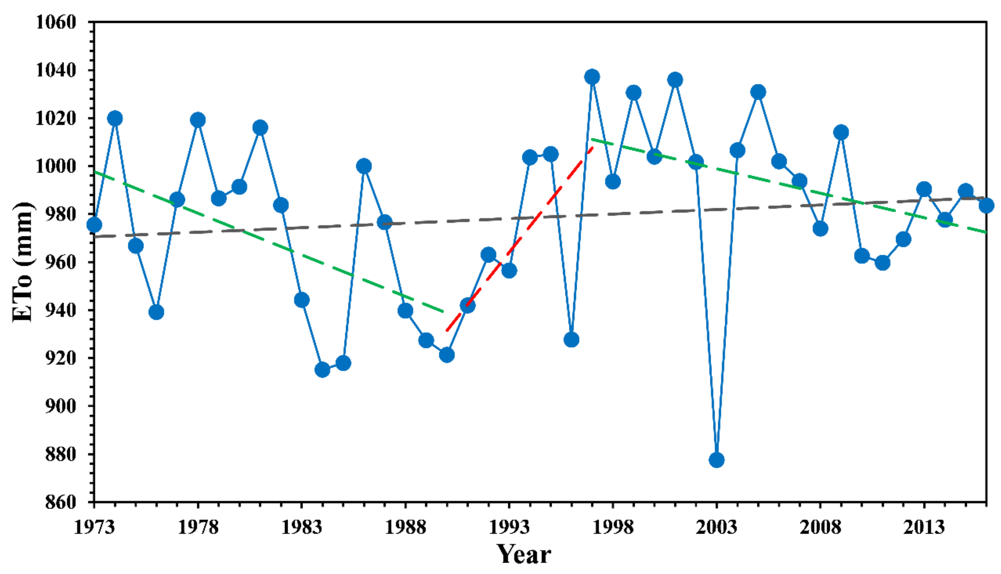
The results of breakpoint detection for ETo time series are shown in Figure 6. ETo did not monotonously decrease or increase during 1973–2016, and there were apparent breakpoints in 1990 and 1997. According to these two time points, the study period from 1973 to 2016 (WP) was divided into three subperiods: 1973–1990 (P1), 1990–1997 (P2), and 1997–2016 (P3). Then, the ETo trend and each climatic factor trend during every time period were examined by TFPW MK test (Figure 7). During the three subperiods, annual ETo first considerably decreased (p < 0.01), then insignificantly increased, and finally significantly decreased (p < 0.05). The effects of the significant decreasing trends in the first and third subperiods were counteracted by the increasing trend in the second subperiod, resulting in an overall slight increasing trend with an average rate of 0.302 mm yr−1 for WP.
Before explaining why ETo shifted during 1973–2016 (Section 3.4), we computed the trends of the underlying climatic driving factors of the whole area during each period (Figure 7). For WP, RH, SD, and WS all showed significant decreasing trends (p < 0.001) at rates of −0.089% yr−1, −0.019 h yr−1, and −0.007 m s−1 yr−1, respectively. Tmax and Tmin displayed significant increasing trends (p < 0.001) of 0.033 °C·yr−1 and 0.045 °C·yr−1, respectively. RH insignificantly increased (0.038% yr−1) during P1 but turned to continuously decrease during the following subperiods (P2: −0.614%·yr−1; P3: −0.022%·yr−1). SD fell in all subperiods, with the only P3 reaching the 0.001 significance level. Tmax during P1 (0.007 °C·yr−1) and P2 (0.094 °C·yr−1) insignificantly increased but insignificantly decreased (−0.028 °C·yr−1) during P3. For all subperiods, Tmin continuously climbed at rates of 0.039 °C·yr−1, 0.086 °C yr−1, and 0.002 °C yr−1, respectively. WS significantly (p < 0.001) decreased (−0.033 m s−1·yr−1) during P1, while it displayed insignificant increasing trends during P2 (0.041 m·s−1·yr−1) and P3 (0.002 m·s−1·yr−1).
3.3. Spatiotemporal Changes of Sensitivity Coefficients
3.3.1. Along Horizontal Gradients
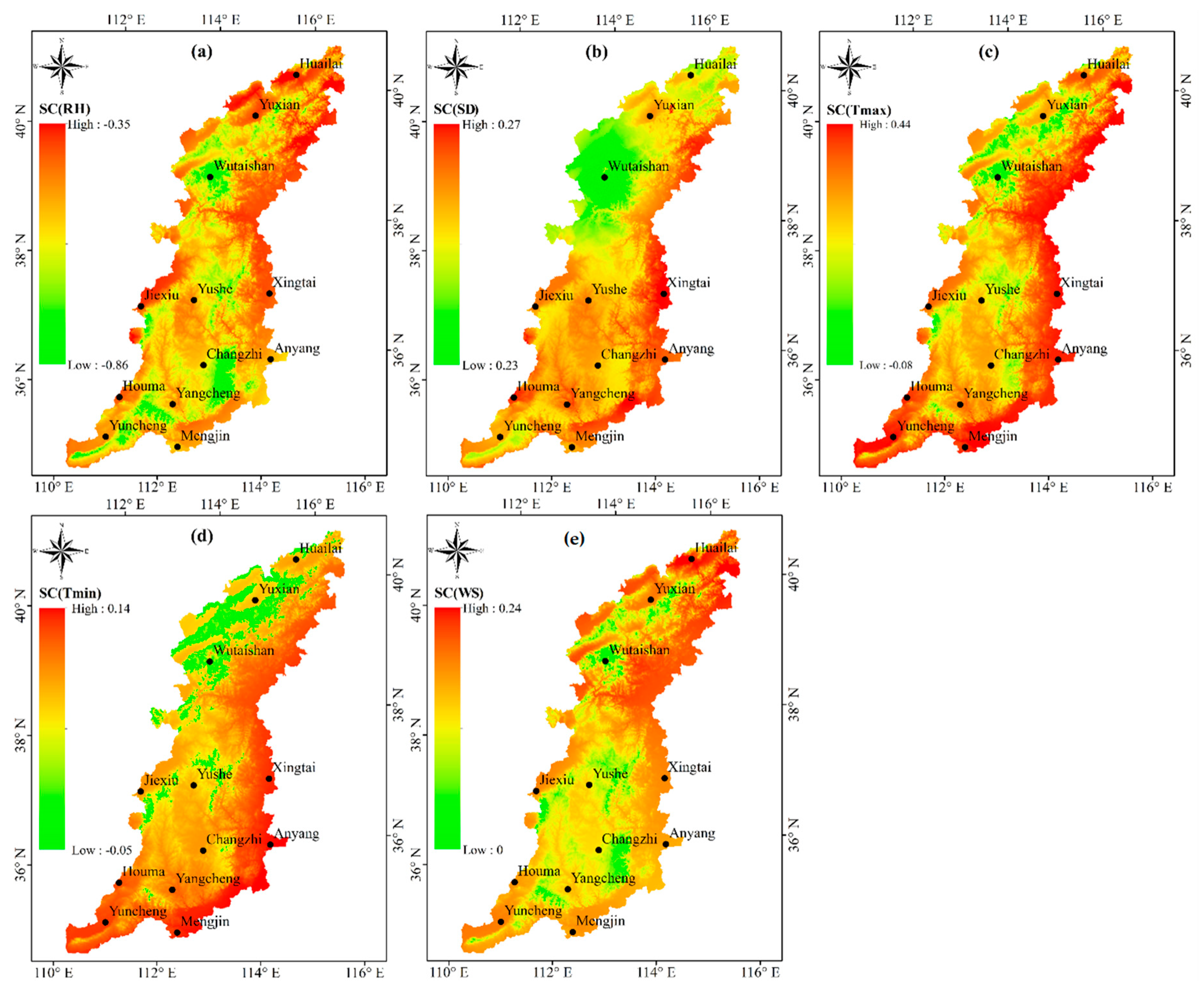
Figure 8 presents the 44-year average sensitivity coefficient of each climatic factor in THM. The sensitivity coefficient of RH (SC(RH), 0.177) was the highest, followed by those of Tmax (SC(Tmax, 0.134), SD (SC(SD), 0.087), WS (SC(WS), 0.065), and the sensitivity coefficient of Tmin (SC(Tmin), 0.026). Nevertheless, SC(RH) was the only sensitivity coefficient with a value below zero across the whole THM, which indicates that an increase in RH would result in a reduction in ETo (Figure 8a). Meanwhile, low values of the SC(RH) were mainly distributed in the north-central and south-central regions, which means ETo had greater sensitivity to the variation in RH in these regions than that in the other region. As seen in Figure 8b, positive SC(SD) was spread throughout the THM, which means that an increase in SD would lead to an increase in ETo. Low values of the SC(SD) were highly concentrated in the northwest region and the nearby region of Wutaishan station. Compared with the SC(RH) and SC(SD), negative and positive SC(Tmax) both can be found in Figure 8c. The SC(Tmax) negative values were gathered in the northwest, and the SC(Tmax) was higher in the eastern plain than that in the western highland. A similar spatial pattern illustrated in the SC(Tmin) map (Figure 8d), the SC(Tmin) in the eastern plain had a higher value than that in the western highland. SC(WS) across the THM was always positive, and the northeast had higher values than the value in the central-north and central-south regions (Figure 8e).
The trends of the sensitivity coefficients of the five climatic factors displayed pronounced differences in horizontal spatial distribution over the past 44 years (Figure 9). The SC(RH) increased markedly for the whole THM but decreased in the south-central area (Figure 9a). Decreasing trends of SC(SD) were found at most THM areas except the northwestern and a small area in the southwest with increasing trends (Figure 9b). The SC(Tmax) experienced an upward trend in the vast west region but declined in the eastern boundary region (Figure 9c). The SC(Tmin) decreased in the northwest region near Yuxian and Wutaishan stations but increased in the remaining areas in THM (Figure 9d). The sensitivity of annual ETo to the changes in WS was strengthened over almost the whole THM, except the southwest region around Yuncheng station, where the SC(WS) slightly decreased (Figure 9e).
3.3.2. Along Vertical Gradients
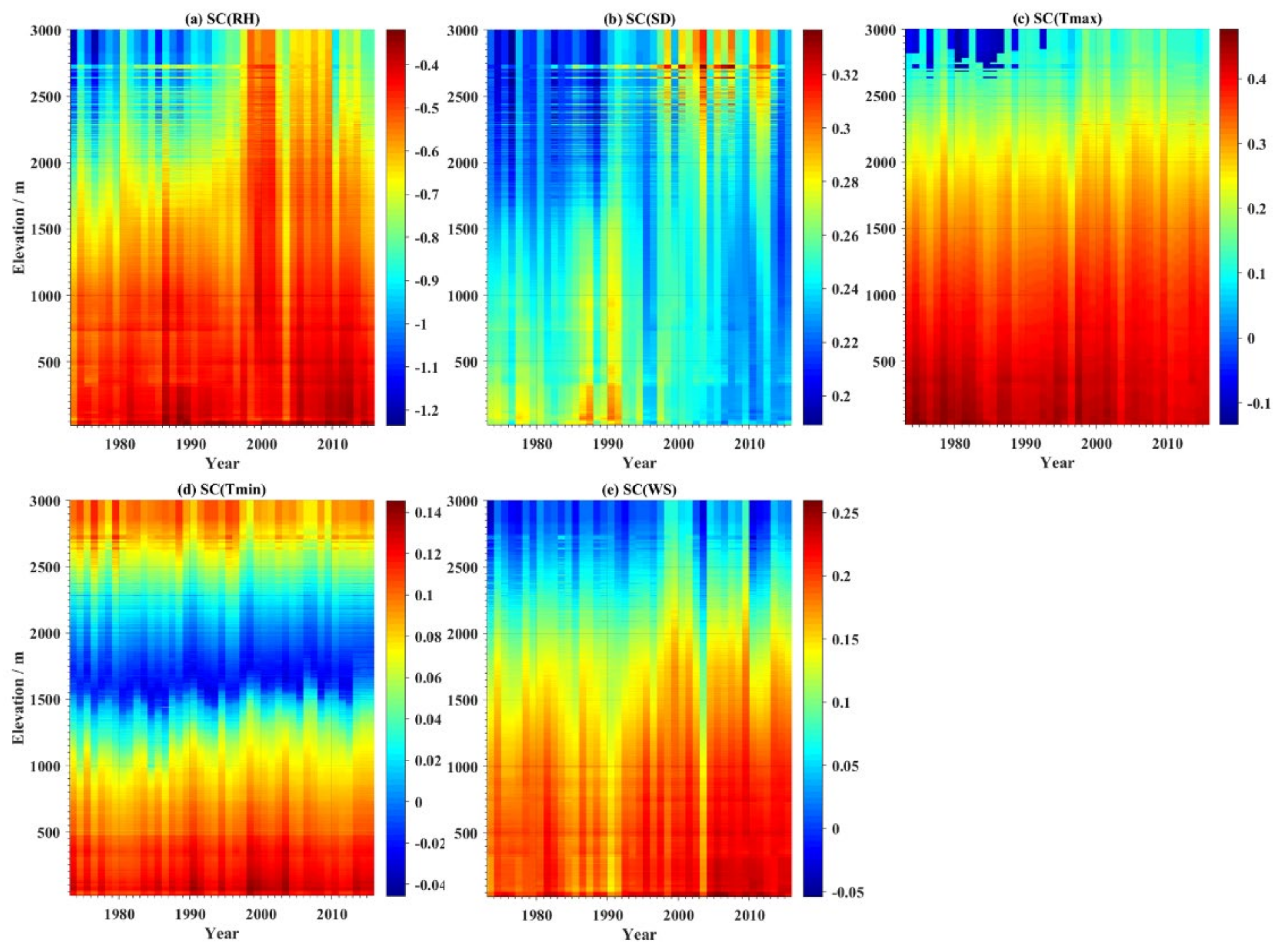
To depict the temporal evolution of sensitivity at different vertical gradients, a Hovmöller diagram [66] was drawn with years along the abscissa and elevation gradients along the ordinate (Figure 10). Moreover, we classified the elevation ranges of the THM into three bands: 0–1250 m (i.e., low elevations), 1250–2250 m (i.e., middle elevations), and 2250–3000 m (i.e., high elevations) to assist the following interpretation of the results and discussion (Section 4.2). The sensitivity coefficient of each climatic factor in the different altitudinal gradients exhibited evident temporal variations. For SC(RH) above low elevations, there was a turning point in approximately 1997, and the peak value was reached in that year (Figure 10a). It is noteworthy that the SC(RH) was negative in this altitude band in 1997, which means that the sensitivity of ETo to the variation in RH was the lowest in that year. At low elevations, the SC(RH) maintained a low absolute value and evolved stably over time. In contrast to the SC(RH), the SC(SD) did not show a prominent vertical spatial feature, and temporal vibrations existed at all elevations bands (Figure 10b). At high elevations, the SC(SD) moved with an undulating curve from 1973 to 2016. At low elevations, the SC(SD) increased in volatility approximately before 1986 but then decreased. Figure 10c shows an apparent altitudinal pattern in SC(Tmax). The annual ETo at higher elevations had lower sensitivity to changes in Tmax, and this vertical distribution did not markedly change with time. However, sporadic negative SC(Tmax) can be found at high elevations. A visually vertical pattern in the SC(Tmin) is presented in Figure 10d; the low-sensitivity belt formed at middle elevations cut the continuous high-sensitivity band. The SC(WS) at middle and high elevations was lower than that at the low elevations over the whole study period (Figure 10e). At the middle elevations, SC(WS) temporally proceeded in a wave shape, where ridges occurred in approximately 1981 and 1999, and troughs occurred in around 1990 and 2012.
3.4. Dominant Factors of ETo in Different Periods
Table 2 shows the regression coefficients derived from a multiple linear model and relative contributions of different climatic factors to ETo for THM during each period. In all periods, the regression coefficients of RH were negative, suggesting that RH was inversely correlated to ETo. However, in contrast with the regression coefficients of RH, all of the regression coefficients of SD, Tmax, and WS were positive, meaning that an increase in ETo occurred if one of the three factors increased in any period. In terms of the relative contributions, Tmin ranked last out of all the influencing factors of ETo, indicating that Tmin was the least important to ETo compared with the other four climatic factors. During WP, RH was the most important for ETo trend, followed by SD, WS, Tmax, and Tmin. The decreasing SD and WS should have led to a decrease in ETo, with relative contributions of 24.64% and 20.60%, respectively. However, the decrease in RH and the increases in Tmax, and Tmin led to a slight increase in ETo, with relative contributions of 30.08%, 13.24%, and 11.43%, respectively. During P1, the increasing Tmax and Tmin should have caused an increase in ETo, with relative contributions of 11.19% and 2.38%, respectively. However, the increasing RH and the decreasing SD and WS caused a significant reduction in ETo, with relative contributions of 26.02%, 40.55%, and 19.85%, respectively. During P2, the decreasing SD and the increasing Tmin should have resulted in a decrease in ETo with relative contributions of 18.25% and 3.69%, respectively. However, the decrease in RH and the increases in Tmax and WS resulted in a considerable increase in ETo, with relative contributions of 7.28%, 56.89%, and 13.87%, respectively. During P3, the decreasing RH and the increasing Tmin and WS should have caused an increase in ETo, with relative contributions of 21.66%, 2.07%, and 17.24%, respectively. However, the decreases in SD and Tmax caused a significant reduction in ETo, with relative contributions of 42.15% and 16.88%, respectively.
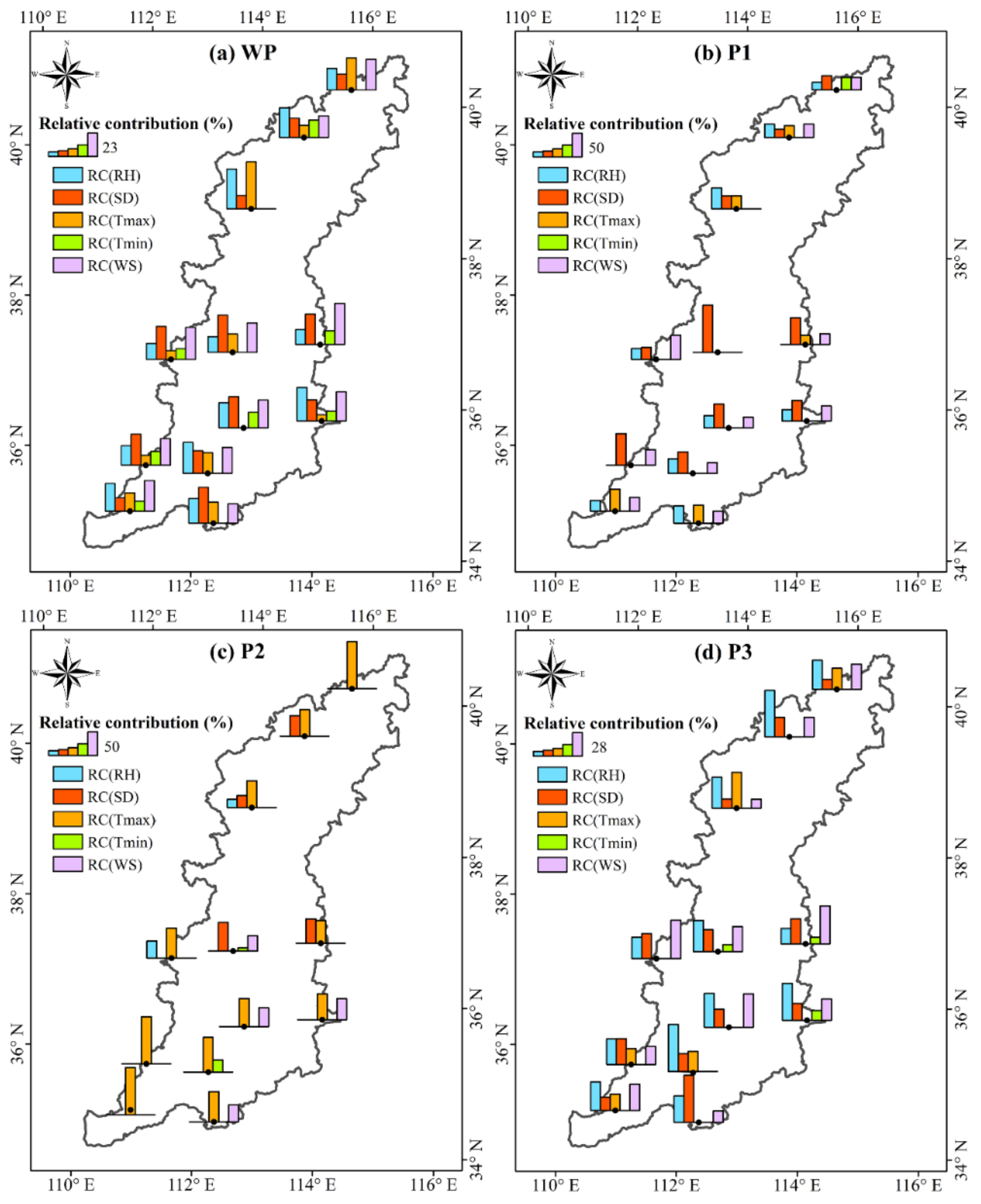
To know how and with what magnitudes the importance of climatic factors to ETo vary in space and time, the relative contributions of all the climatic factors to ETo at the 12 stations were calculated using stepwise multiple regression, yielding Figure 11. During WP, the increasing WS mainly controlled the rising trend of the ETo series at Xingtai station, which is in the eastern region (Figure 11a). For the 6 stations (i.e., 50% of the total stations) located in the south part, RH, WS, and SD had higher relative contributions than temperature (including Tmax and Tmin). Moreover, WS and SD were the most critical factors for ETo at 3 stations (i.e., 25% of all the stations; Jiexiu, Yushe, and Xingtai) of the central region (Figure 9b). During P1, ETo at half of the stations (i.e., 6 stations) located in the central southern area was mainly impacted by SD. Moreover, SD was the only climatic factor that affected the ETo of Yushe station (Figure 11c). During P2, the annual ETo of approximately all the stations (i.e., 91.7% of the stations; 11 stations) were primarily influenced by Tmax, but WS was also critical to ETo for 33.3% of the total stations (i.e., 4 stations) in the eastern area. During P3, RH was the most crucial factor in 2 stations (i.e., Huailai and Yuxian) in the northern area (Figure 11e). Closely resembling WP, WS, RH, and SD were the first three contributors to ETo for the 5 stations (i.e., 41.7% of all the stations) located in the middle southern area. However, SD and RH made the most enormous contribution to ETo of Mengjin station (i.e., 8.3% of all the stations) in the southernmost area.
4. Discussion
4.1. Changes of ETo and Climatic Factors
The distribution of annual ETo showed a strong spatial gradient in the THM during the 44-year period, with the highest value in the western highland and the lowest value in the eastern hilly land and plain. Meanwhile, we found distinct spatial differences of ETo trends in the THM from 1973 to 2016. ETo in the northeast part neighboring Beijing exhibited a decreasing trend, which agreed with the findings of Han et al. [67] and Shan et al. [5]. In addition, ETo in the western part of the THM exhibited pronounced growth, which was also found in the similar regions, e.g., the eastern region of the Loess Plateau [34] and the middle reaches of the Yellow River Basin [22,68]. Moreover, in accordance with the findings of Wang et al. [69], air temperature exhibited a significant (p < 0.001) increasing trend in the THM from 1973–2016. According to the observations of Fan et al. [53], climatic variability combined with anthropogenic emissions of greenhouse gases caused increases in Tmax (0.02 °C yr−1) and Tmin (0.037 °C yr−1) in China during 1956–2016. The rates of the increases in Tmax (0.033 °C yr−1) and Tmin (0.045 °C yr−1) from our observations indicated that the warming rate of the THM was 1.5 times greater than the national average rate. The augmentation of Tmax may be explained by the increased absorption of solar radiation during the daytime, and enhancement of Tmin is possibly due to the reduced nocturnal cloud cover [70,71]. The dramatic decrease in WS (stilling) has been found to prevail throughout the world [72] and was also found in the THM. Locally, the increase in the underlying surface roughness due to the enhancement of vegetation coverage [73,74] must be the cause of the decrease in WS [75] under the implementation of the Beijing-Tianjin Dust Storms Source Control Project and Afforestation in Taihang Mountains Project. The solar dimming caused by the increase in cloud cover can also contribute to the decreased SD [31]. In addition, aggregated aerosols and pollution could be a plausible explanation [76,77], considering the rapid economic development of the vicinal Beijing-Tianjin-Hebei metropolitans [78].
Climatic conditions change markedly with elevation, and the trend of temperature was always considered as a preferred examiner of climate change [30,79]. Consistent with the conclusion of Pepin et al. [30], the rate of warming is amplified with elevation because the increasing rate of Tmax (0.0034 °C·yr−1·m−1) with increasing elevation was approximately twice as great as the decreasing rate of Tmin (−0.0019 °C·yr−1·m−1) with increasing elevation. “Climate change” means more than “global warming”, and changes in the other climatic factor also impact ETo. In this study, WS was found to decline more rapidly at higher elevations than lower elevations. This phenomenon can also be found in mountainous regions of Switzerland and central China [80] and even at the scale of the entirety of China [81]. In addition, a lower absolute decreasing rate of RH at higher elevation implies the air there becoming drier more slowly than that at lower elevation. Compared with other Chinese regions with middle or low elevations, the Tibetan Plateau also got drier more slowly [53]. Although change rates of temperature, WS and RH all showed an elevation-dependent feature, the change rate of SD did not show a clear. Impacted by the combination of changes in all the climatic factors, no clear elevational gradient was found in the change rate of ETo.
4.2. Sensitivity of ETo to Variations in Climatic Factors
Sensitivity analysis showed that regional average ETo was most sensitive to the changes in RH, and similar conclusions were also drawn by studies of other regions, e.g., the Yangtze River Basin [21], Yellow River Basin [51], Haihe River basin [82] of China, the coastal region of Iran [83] and Spain [17]. The higher sensitivity of ETo to the variation in Tmax than to the variation in Tmin could be explained by the fact that daytime ET makes up a larger portion of the total ET than nocturnal ET. In essence, daily ET cycles are driven by the available energy, and maximum energy (solar radiation) is commonly measured in the daytime when Tmax is also recorded [17]. Tmin is recorded at night when less ET is generated. Differing from most semiarid and semi-humid regions of China, ETo of the THM exhibited the second highest sensitivity to the variation in Tmax, not to the variation in SD [23,49]. Meanwhile, the increasing trend of the sensitivity coefficients of all climatic factors, excluding SD, indicates that ETo became more sensitive to the climate change in the THM.
As discussed above, the sensitivity of ETo to climatic factors is known to vary spatially among climate zones [23,53,78]. Here, we also should notice that elevation strongly impacts climatic condition, thereby affecting ETo and its sensitivity to climatic factors [79]. However, the vertical pattern of sensitivity of ETo was seldom discussed. One of the main findings of our study is that an obvious vertical zonal pattern existed in the sensitivity coefficients of all the climatic factors, except SC(SD) with equal value (0.24) among the three elevation bands. Moreover, the SC(SD) at every elevation band irregularly varied with time in THM. The possible reason is that SD was also affected by slope and aspect [33,36,79] besides elevation. In this study, higher elevations had higher SC(RH) (i.e., −0.47 at low elevations, −0.58 at middle elevations and −0.74 at high elevations). This result is consistent with the study of the Qilian Mountains of northwestern China [79]. Meanwhile, ETo at high elevations was most sensitive to the change in RH (0.74). However, there are some differences between the results of Yang et al. [79] and our results that SC(WS) increased as elevation increased in the Qilian Mountains but decreased as elevation increased in THM. The data Yang et al. [79] used were from five in situ stations located in a small catchment with an area of 23.1 km2, but meteorological data in this study were collected from national meteorological stations. The relationship between sensitivity of ETo and elevation may be influenced by data source. In agreement with the findings of Xu et al. [33] and Liu et al. [20], SC(Tmax) in THM showed a similar negative linear relationship with elevation. However, SC(Tmin) formed a low-value (0.013) belt at middle elevations of THM, and the SC(Tmin) at low and high elevations were 0.091 and 0.044, respectively. This is inconsistent with the results for the Jing River Basin [33] that SC(Tmin) and elevation were linear negative correlated. The sensitivity study of Xu et al. [33] was conducted at site level, but this study was conducted at region level. Difference in level may impact the sensitivity of ETo. In this study, along with the time axis, the SC(RH) and SC(WS) at high elevations exhibited a greater amplitude of variation than those at low altitudes. The unstable temporal evolution of these factors in the THM confirmed the volatility of mountainous hydrometeorology.
4.3. Changes of Dominant Factors of ETo
Several recent studies demonstrated that the (relative or actual) contributions of different climatic factors changed with time rather than staying constant [22,33,37,67]. Before exploring the temporal patterns of the relative contributions, the rationality of dividing the average climatic period based on breakpoints needs to be verified. The results of the breakpoint detection indicated that ETo of the THM shifted in 1990 and 1997, instead of monotonously increasing from 1973 to 2016. The two inflection points presented here coincide with the conclusions in Han et al. [67] and She et al. [22], which also reported that the change in ETo showed an abrupt change in approximately the years of 1990 and 1997 at nearby regions. Nevertheless, these results are different from the results of change-points detection of Wang et al. (2018), who found that the ETo series mutated in 1982, which may be due to the inability of the small basin to adequately reflect the hydrometeorological conditions of the whole THM. An additional eye inspection of the series confirmed a remarkable difference between the ETo trends before and after each time point.
According to the differences between ETo trend and each climatic factor trend, we can know that ETo did not keep pace with the climatic factors in the THM, which indicates that the combined effect of the five climatic factors changed ETo trend. For all the periods (including the whole study period and three subperiods), Tmin had the least impact on annual ETo in the THM, which is coincident with the results of Li et al. [34]. Moreover, we found that the “evaporation paradox” phenomenon in the first warming subperiod was covered by the 44-year long-term overall increasing ETo series. Why did the contradiction occur during the period of 1973–1990? There are three reasons for this: (1) The decrease in SD played a considerable role (40.55%) to the decrease in ETo of this subperiod; (2) the decrease in wind speed restrained the transfer of vapor from the leaf surface of crops to the atmosphere [8]; and (3) the wetter the air (i.e., higher RH), the lower the vapor pressure and the smaller the difference between the vapor pressure of ambient air and that of air inside the stoma, resulting in a reduction in ETo [34]. In our study, we also found that SD was the dominate factor of the decreasing ETo both during the first subperiod (1973–1990) and the third subperiod (1997–2016). These results are consistent with the findings of She et al. [22] for the middle reaches of the Yellow River Basin, located in the southwest of the THM, but disagree with the findings of Han et al. [67] for the Jing-Jin-Ji region, located in the northeast of the THM, which may be induced by the spatial differences. However, the increasing Tmax became the largest contributor to the increase in ETo of the second time period (1990–1997). Irmak et al. (2006) explained that since saturation vapor pressure is an exponential function of temperature and ETo is a linear function of the vapor pressure deficit, a fairly large increase in ETo is expected for an increase in temperature in the semiarid environments.
5. Conclusions
Temporal and spatial trends of ETo and its determining climatic factors were evaluated based on the data from 12 meteorological stations of the THM during 1973–2016, utilizing TFPW MK, the breakpoint detection method, sensitivity coefficient approach, and multiple stepwise regression. Over the whole THM, annual ETo increased in the extensive area, except the northeast part and southwest part. In addition, regional average ETo shifted in 1990 and 1997, and an “evaporation paradox” occurred in 1973–1990. For the whole study period, ETo was most sensitive to the variations in RH and Tmax. ETo was becoming more sensitive to the variations in RH, Tmin, and WS. Besides conventional horizontal gradients, the vertical gradients of change rate of various climatic factors and sensitivity of ETo were also researched. Viewed from vertical direction, the higher the elevation, the slower the decreasing rate of RH, the rapider the increasing rate of temperature, and the rapider the decreasing rate of WS. However, ETo at higher elevation had higher sensitivity to RH and lower sensitivity to WS and Tmax. ETo at middle elevations had the lowest sensitivity to Tmin among three elevation bands. For the climatic reason of changes in ETo of different periods, RH and SD governed the increasing ETo of the whole period and the decreasing ETo of two subperiods (i.e., 1973–1990 and 1997–2016). However, Tmax and SD exerted the most influence on the increasing ETo of 1990–1997. In the future, the relationship ETo with saturation vapor pressure deficit needs to be investigated due to its important role to ETo.
Our study confirmed that ETo at high elevations markedly responded to the climate change, with more variations than that at lower elevations. The results of this study can serve as a reference for hydrometeorology research in other mountainous areas; nevertheless, the irregular temporal rainfall intensification should receive more attention.
Author Contributions
T.K. analyzed the data and wrote the manuscript. Z.L. collected data, processed data and drew the figure. Y.G. supervised, review and edit this paper. All authors have read and agreed to the published version of the manuscript.
Funding
This research was funded by [National Key Project for Basic Research] grant number [2015CB452705] and [National Key Project for Research and Development] grant number [2016YFC0501605].
Institutional Review Board Statement
Not applicable.
Informed Consent Statement
Not applicable.
Data Availability Statement
Not applicable.
Acknowledgments
Our research was jointly funded by the National Key Project for Basic Research (973) (2015CB452705) and the National Key Project for Research and Development (2016YFC0501605). We thank the anonymous reviewers and the Editor for their suggestions, which substantially improved the manuscript.
Conflicts of Interest
The authors declare no conflict of interest.
References
- Goyal, R. Sensitivity of evapotranspiration to global warming: A case study of arid zone of Rajasthan (India). Agric. Water Manag. 2004, 69, 1–11. [Google Scholar] [CrossRef]
- Kingston, D.G.; Todd, M.C.; Taylor, R.G.; Thompson, J.R.; Arnell, N.W. Uncertainty in the estimation of potential evapotranspiration under climate change. Geophys. Res. Lett. 2009, 36, 6. [Google Scholar] [CrossRef] [Green Version]
- Laghari, A.N.; Vanham, D.; Rauch, W. To what extent does climate change result in a shift in Alpine hydrology? A case study in the Austrian Alps. Hydrol. Sci. J. 2011, 57, 103–117. [Google Scholar] [CrossRef]
- Saadi, S.; Todorovic, M.; Tanasijevic, L.; Pereira, L.S.; Pizzigalli, C.; Lionello, P. Climate change and Mediterranean agriculture: Impacts on winter wheat and tomato crop evapotranspiration, irrigation requirements and yield. Agric. Water Manag. 2015, 147, 103–115. [Google Scholar] [CrossRef]
- Shan, N.; Shi, Z.; Yang, X.; Gao, J.; Cai, D. Spatiotemporal trends of reference evapotranspiration and its driving factors in the Beijing–Tianjin Sand Source Control Project Region, China. Agric. For. Meteorol. 2015, 200, 322–333. [Google Scholar] [CrossRef]
- Monteith, J.L. Evaporation and environment. In Symposia of the Society for Experimental Biology; Cambridge University Press (CUP): Cambridge, MA, USA, 1965. [Google Scholar]
- Fisher, J.B.; Melton, F.; Middleton, E.; Hain, C.; Anderson, M.; Allen, R.; McCabe, M.F.; Hook, S.; Baldocchi, D.; Townsend, P.A.; et al. The future of evapotranspiration: Global requirements for ecosystem functioning, carbon and climate feedbacks, agricultural management, and water resources. Water Resour. Res. 2017, 53, 2618–2626. [Google Scholar] [CrossRef]
- Allen, R.G.; Pereira, L.S.; Raes, D.; Smith, M. Crop Evapotranspiration-Guideline for Computing Crop Water Requirement-FAO Irrigation and Drainage Paper 56; Food and Agriculture Organisation: Rome, Italy, 1998; Volume 300, p. D05109. [Google Scholar]
- Anderson, M.C.; Kustas, W.P.; Norman, J.M.; Hain, C.R.; Mecikalski, J.R.; Schultz, L.; González-Dugo, M.P.; Cammalleri, C.; D’Urso, G.; Pimstein, A.; et al. Mapping daily evapotranspiration at field to continental scales using geostationary and polar orbiting satellite imagery. Hydrol. Earth Syst. Sci. 2011, 15, 223–239. [Google Scholar] [CrossRef] [Green Version]
- Li, Z.; Zheng, F.-L.; Liu, W. Spatiotemporal characteristics of reference evapotranspiration during 1961–2009 and its projected changes during 2011–2099 on the Loess Plateau of China. Agric. For. Meteorol. 2012, 154, 147–155. [Google Scholar] [CrossRef]
- Aouissi, J.; Benabdallah, S.; Chabaâne, Z.L.; Cudennec, C. Evaluation of potential evapotranspiration assessment methods for hydrological modelling with SWAT—Application in data-scarce rural Tunisia. Agric. Water Manag. 2016, 174, 39–51. [Google Scholar] [CrossRef]
- Stocker, T.; Qin, D.; Plattner, G.; Tignor, M.; Allen, S.; Boschung, J.; Nauels, A.; Xia, Y.; Bex, V.; Midgley, P. IPCC, 2013: Summary for Policymakers in Climate Change 2013: The Physical Science Basis, Contribution of Working Group I to the Fifth Assessment Report of the Intergovernmental Panel on Climate Change; Cambridge University Press: Cambridge, MA, USA, 2013. [Google Scholar]
- Peterson, T.C.; Golubev, V.S.; Groisman, P. Evaporation losing its strength. Nature 1995, 377, 687–688. [Google Scholar] [CrossRef]
- Rayner, D.P. Wind Run Changes: The Dominant Factor Affecting Pan Evaporation Trends in Australia. J. Clim. 2007, 20, 3379–3394. [Google Scholar] [CrossRef]
- Cong, Z.T.; Yang, D.W.; Ni, G.H. Does evaporation paradox exist in China? Hydrol. Earth Syst. Sci. 2009, 13, 357–366. [Google Scholar] [CrossRef] [Green Version]
- Brutsaert, W.; Parlange, M. Hydrologic cycle explains the evaporation paradox. Nature 1998, 396, 30. [Google Scholar] [CrossRef]
- Vicente-Serrano, S.M.; Azorin-Molina, C.; Sanchez-Lorenzo, A.; Revuelto, J.; Morán-Tejeda, E.; Lopez-Moreno, I.; Espejo, F. Sensitivity of reference evapotranspiration to changes in meteorological parameters in Spain (1961–2011). Water Resour. Res. 2014, 50, 8458–8480. [Google Scholar] [CrossRef] [Green Version]
- Irmak, S.; Payero, J.O.; Martin, D.L.; Irmak, A.; Howell, T.A. Sensitivity Analyses and Sensitivity Coefficients of Standardized Daily ASCE-Penman-Monteith Equation. J. Irrig. Drain. Eng. 2006, 132, 564–578. [Google Scholar] [CrossRef]
- Yin, Y.; Wu, S.; Chen, G.; Dai, E. Attribution analyses of potential evapotranspiration changes in China since the 1960s. Theor. Appl. Clim. 2010, 101, 19–28. [Google Scholar] [CrossRef]
- Liu, C.; Zhang, D.; Liu, X.; Zhao, C. Spatial and temporal change in the potential evapotranspiration sensitivity to meteorological factors in China (1960–2007). J. Geogr. Sci. 2012, 22, 3–14. [Google Scholar] [CrossRef]
- Gong, L.; Xu, C.-Y.; Chen, D.; Halldin, S.; Chen, Y.D. Sensitivity of the Penman–Monteith reference evapotranspiration to key climatic variables in the Changjiang (Yangtze River) basin. J. Hydrol. 2006, 329, 620–629. [Google Scholar] [CrossRef]
- She, D.; Xia, J.; Zhang, Y. Changes in reference evapotranspiration and its driving factors in the middle reaches of Yellow River Basin, China. Sci. Total Environ. 2017, 607–608, 1151–1162. [Google Scholar] [CrossRef]
- Zheng, C.; Wang, Q. Spatiotemporal pattern of the global sensitivity of the reference evapotranspiration to climatic variables in recent five decades over China. Stoch. Environ. Res. Risk Assess. 2015, 29, 1937–1947. [Google Scholar] [CrossRef]
- Liu, T.; Li, L.; Lai, J.; Liu, C.; Zhuang, W. Reference evapotranspiration change and its sensitivity to climate variables in southwest China. Theor. Appl. Clim. 2016, 125, 499–508. [Google Scholar] [CrossRef]
- Tabari, H.; Marofi, S.; Aeini, A.; Hosseinzadehtalaei, P.; Mohammadi, K. Trend analysis of reference evapotranspiration in the western half of Iran. Agric. For. Meteorol. 2011, 151, 128–136. [Google Scholar] [CrossRef]
- Martínez-Cob, A.; Tejero-Juste, M. A wind-based qualitative calibration of the Hargreaves ET0 estimation equation in semiarid regions. Agric. Water Manag. 2004, 64, 251–264. [Google Scholar] [CrossRef] [Green Version]
- Messerli, B.; Ives, J.D. Mountains of the World: A Global Priority; The Parthenon Publishing Group: New York, NY, USA, 1997. [Google Scholar]
- Viviroli, D.; Archer, D.R.; Buytaert, W.; Fowler, H.J.; Greenwood, G.B.; Hamlet, A.F.; Huang, Y.; Koboltschnig, G.; Litaor, M.I.; López-Moreno, J.I.; et al. Climate change and mountain water resources: Overview and recommendations for research, management and policy. Hydrol. Earth Syst. Sci. 2011, 15, 471–504. [Google Scholar] [CrossRef] [Green Version]
- Krishnaswamy, J.; John, R.; Joseph, S. Consistent response of vegetation dynamics to recent climate change in tropical mountain regions. Glob. Chang. Biol. 2014, 20, 203–215. [Google Scholar] [CrossRef]
- Pepin, N.; Bradley, R.S.; Diaz, H.F.; Baraer, M.; Caceres, E.B.; Forsythe, N.; Fowler, H.; Greenwood, G.; Hashmi, M.Z.; Liu, X.D.; et al. Elevation-dependent warming in mountain regions of the world. Nat. Clim. Chang. 2015, 5, 424–430. [Google Scholar] [CrossRef] [Green Version]
- Roderick, M.L.; Farquhar, G.D. The Cause of Decreased Pan Evaporation over the Past 50 Years. Science 2002, 298, 1410–1411. [Google Scholar] [CrossRef] [PubMed]
- Giorgi, F.; Hurrell, J.W.; Marinucci, M.R.; Beniston, M. Elevation dependency of the surface climate change signal: A model study. J. Clim. 1997, 10, 288–296. [Google Scholar] [CrossRef] [Green Version]
- Xu, L.; Shi, Z.; Wang, Y.; Zhang, S.; Chu, X.; Yu, P.; Xiong, W.; Zuo, H.; Wang, Y. Spatiotemporal variation and driving forces of reference evapotranspiration in Jing River Basin, northwest China. Hydrol. Process. 2015, 29, 4846–4862. [Google Scholar] [CrossRef]
- Li, C.; Wu, P.; Li, X.; Zhou, T.; Sun, S.; Wang, Y.; Luan, X.; Yu, X. Spatial and temporal evolution of climatic factors and its impacts on potential evapotranspiration in Loess Plateau of Northern Shaanxi, China. Sci. Total Environ. 2017, 589, 165–172. [Google Scholar] [CrossRef]
- Zhang, X.; Wang, L.; Chen, D. How does temporal trend of reference evapotranspiration over the Tibetan Plateau change with elevation? Int. J. Clim. 2019, 39, 2295–2305. [Google Scholar] [CrossRef]
- McVicar, T.R.; Van Niel, T.; Li, L.; Hutchinson, M.F.; Mu, X.; Liu, Z. Spatially distributing monthly reference evapotranspiration and pan evaporation considering topographic influences. J. Hydrol. 2007, 338, 196–220. [Google Scholar] [CrossRef]
- Fan, Z.-X.; Thomas, A. Decadal changes of reference crop evapotranspiration attribution: Spatial and temporal variability over China 1960–2011. J. Hydrol. 2018, 560, 461–470. [Google Scholar] [CrossRef]
- Sakakibara, K.; Tsujimura, M.; Song, X.; Zhang, J. Spatiotemporal variation of the surface water effect on the groundwater recharge in a low-precipitation region: Application of the multi-tracer approach to the Taihang Mountains, North China. J. Hydrol. 2017, 545, 132–144. [Google Scholar] [CrossRef]
- Yang, Y.; Watanabe, M.; Sakura, Y.; Changyuan, T.; Hayashi, S. Groundwater-table and recharge changes in the Piedmont region of Taihang Mountain in Gaocheng City and its relation to agricultural water use. Water SA 2002, 28, 171–178. [Google Scholar] [CrossRef] [Green Version]
- Cai, Q.; Liu, Y. Climatic response of Chinese pine and PDSI variability in the middle Taihang Mountains, north China since 1873. Trees 2013, 27, 419–427. [Google Scholar] [CrossRef]
- Editorial Committee of Yearbook of China’s Poverty Alleviation and Development (CPAD). The Yearbook of China’s Poverty Alleviation and Development; Unity Press: Beijing, China, 2015. [Google Scholar]
- Liu, Y.; Liu, J.-L.; Zhou, Y. Spatio-temporal patterns of rural poverty in China and targeted poverty alleviation strategies. J. Rural Stud. 2017, 52, 66–75. [Google Scholar] [CrossRef]
- Li, W. Degradation and restoration of forest ecosystems in China. For. Ecol. Manag. 2004, 201, 33–41. [Google Scholar] [CrossRef]
- Yang, X.; Yan, D.; Liu, C. Natural Regeneration of Trees in Three Types of Afforested Stands in the Taihang Mountains, China. PLoS ONE 2014, 9, e108744. [Google Scholar] [CrossRef]
- Geng, S.; Shi, P.; Song, M.; Zong, N.; Zu, J.; Zhu, W. Diversity of vegetation composition enhances ecosystem stability along elevational gradients in the Taihang Mountains, China. Ecol. Indic. 2019, 104, 594–603. [Google Scholar] [CrossRef]
- Li, W.; Tan, M. NDVI variation tendency under different slopes in Taihang Mountain. Zhongguo Shengtai Nongye Xuebao/Chin. J. Eco-Agric. 2017, 25, 509–519. [Google Scholar]
- China Meteorological Administration (CMA). Automatic Climatic Station Requirements Specification; China Meteorological Administration Integrated Observation Division, China Methodological Press: Beijing, China, 2014. [Google Scholar]
- Hutchinson, M.F. Interpolating mean rainfall using thin plate smoothing splines. Int. J. Geogr. Inf. Syst. 1995, 9, 385–403. [Google Scholar] [CrossRef]
- Zhang, X.; Kang, S.; Zhang, L.; Liu, J. Spatial variation of climatology monthly crop reference evapotranspiration and sensitivity coefficients in Shiyang river basin of northwest China. Agric. Water Manag. 2010, 97, 1506–1516. [Google Scholar] [CrossRef]
- Shadmani, M.; Marofi, S.; Roknian, M. Trend Analysis in Reference Evapotranspiration Using Mann-Kendall and Spearman’s Rho Tests in Arid Regions of Iran. Water Resour. Manag. 2012, 26, 211–224. [Google Scholar] [CrossRef] [Green Version]
- Wang, W.; Shao, Q.; Peng, S.; Xing, W.; Yang, T.; Luo, Y.; Yong, B.; Xu, J. Reference evapotranspiration change and the causes across the Yellow River Basin during 1957–2008 and their spatial and seasonal differences. Water Resour. Res. 2012, 48, 5. [Google Scholar] [CrossRef]
- Wang, W.; Xing, W.; Shao, Q.; Yu, Z.; Peng, S.; Yang, T.; Yong, B.; Taylor, J.; Singh, V.P. Changes in reference evapotranspiration across the Tibetan Plateau: Observations and future projections based on statistical downscaling. J. Geophys. Res. Atmos. 2013, 118, 4049–4068. [Google Scholar] [CrossRef]
- Fan, J.; Wu, L.; Zhang, F.; Xiang, Y.; Zheng, J. Climate change effects on reference crop evapotranspiration across different climatic zones of China during 1956–2015. J. Hydrol. 2016, 542, 923–937. [Google Scholar] [CrossRef]
- Gao, Z.; He, J.; Dong, K.; Li, X. Trends in reference evapotranspiration and their causative factors in the West Liao River basin, China. Agric. For. Meteorol. 2017, 232, 106–117. [Google Scholar] [CrossRef]
- Mann, H.B. Nonparametric Tests Against Trend. Econometrica 1945, 13, 245–259. [Google Scholar] [CrossRef]
- Kendall, M.G. Rank Correlation Methods; Charles Griffin: London, UK, 1975. [Google Scholar]
- Von Storch, H. Misuses of statistical analysis in climate research. In Analysis of Climate Variability: Applications of Statistical Techniques; Springer: Berlin, Germany, 1999. [Google Scholar]
- Yue, S.; Pilon, P.; Phinney, B.; Cavadias, G. The influence of autocorrelation on the ability to detect trend in hydrological series. Hydrol. Process. 2002, 16, 1807–1829. [Google Scholar] [CrossRef]
- Aziz, O.I.A.; Burn, D.H. Trends and variability in the hydrological regime of the Mackenzie River Basin. J. Hydrol. 2006, 319, 282–294. [Google Scholar] [CrossRef]
- Sun, S.; Chen, H.; Wang, G.; Li, J.; Mu, M.; Yan, G.; Xu, B.; Huang, J.; Wang, J.; Zhang, F.; et al. Shift in potential evapotranspiration and its implications for dryness/wetness over Southwest China. J. Geophys. Res. Atmos. 2016, 121, 9342–9355. [Google Scholar] [CrossRef] [Green Version]
- Priyadarshana, W.J.R.M.; Sofronov, G. Breakpoint: An R Package for Multiple Break-Point Detection via the Cross-Entropy Method. R Package Version 1.2. 2016. Available online: https://CRAN.R-project.org/package=breakpoint (accessed on 27 October 2021).
- McCuen, R.H. A sensitivity and error analysis CF procedures used for estimating evaporation. J. Am. Water Resour. Assoc. 1974, 10, 486–497. [Google Scholar] [CrossRef]
- Beven, K. A sensitivity analysis of the Penman-Monteith actual evapotranspiration estimates. J. Hydrol. 1979, 44, 169–190. [Google Scholar] [CrossRef]
- Haan, C.T. Statistical Methods in Hydrology; The Iowa State University Press: Iowa City, IA, USA, 1997. [Google Scholar]
- Clow, D. Changes in the Timing of Snowmelt and Streamflow in Colorado: A Response to Recent Warming. J. Clim. 2010, 23, 2293–2306. [Google Scholar] [CrossRef]
- Hovmöller, E. The trough-and-ridge diagram. Tellus 1949, 1, 62–66. [Google Scholar] [CrossRef]
- Han, J.; Wang, J.; Zhao, Y.; Wang, Q.; Zhang, B.; Li, H.; Zhai, J. Spatio-temporal variation of potential evapotranspiration and climatic drivers in the Jing-Jin-Ji region, North China. Agric. For. Meteorol. 2018, 256, 75–83. [Google Scholar] [CrossRef]
- Liu, Q.; Yang, Z.; Cui, B.; Sun, T. The temporal trends of reference evapotranspiration and its sensitivity to key meteorological variables in the Yellow River Basin, China. Hydrol. Process. 2010, 24, 2171–2181. [Google Scholar] [CrossRef]
- Wang, J.; Gao, Y.; Wang, S. Assessing the response of runoff to climate change and human activities for a typical basin in the Northern Taihang Mountain, China. J. Earth Syst. Sci. 2018, 127, 37. [Google Scholar] [CrossRef] [Green Version]
- Duan, A.; Wu, G. Change of cloud amount and the climate warming on the Tibetan Plateau. Geophys. Res. Lett. 2006, 33, 217–234. [Google Scholar] [CrossRef]
- Liu, X.; Yin, Z.-Y.; Shao, X.; Qin, N. Temporal trends and variability of daily maximum and minimum, extreme temperature events, and growing season length over the eastern and central Tibetan Plateau during 1961–2003. J. Geophys. Res. Space Phys. 2006, 111, D19. [Google Scholar] [CrossRef] [Green Version]
- Roderick, M.; Rotstayn, L.; Farquhar, G.; Hobbins, M. On the attribution of changing pan evaporation. Geophys. Res. Lett. 2007, 34, 251–270. [Google Scholar] [CrossRef] [Green Version]
- Jiang, C.; Zhang, H.; Tang, Z.; Labzovskii, L. Evaluating the coupling effects of climate variability and vegetation restoration on ecosystems of the Loess Plateau, China. Land Use Policy 2017, 69, 134–148. [Google Scholar] [CrossRef]
- Xu, G.; Zhang, J.; Li, P.; Li, Z.; Lu, K.; Wang, X.; Wang, F.; Cheng, Y.; Wang, B. Vegetation restoration projects and their influence on runoff and sediment in China. Ecol. Indic. 2018, 95, 233–241. [Google Scholar] [CrossRef]
- Vautard, R.; Cattiaux, J.; Yiou, P.; Thépaut, J.-N.; Ciais, P. Northern Hemisphere atmospheric stilling partly attributed to an increase in surface roughness. Nat. Geosci. 2010, 3, 756–761. [Google Scholar] [CrossRef]
- Streets, D.G.; Yu, C.; Wu, Y.; Chin, M.; Zhao, Z.; Hayasaka, T.; Shi, G. Aerosol trends over China, 1980–2000. Atmos. Res. 2008, 88, 174–182. [Google Scholar] [CrossRef]
- Ning, T.; Li, Z.; Liu, W.; Han, X. Evolution of potential evapotranspiration in the northern Loess Plateau of China: Recent trends and climatic drivers. Int. J. Clim. 2016, 36, 4019–4028. [Google Scholar] [CrossRef]
- Liu, C.; Liu, X.; Zheng, H.; Zeng, Y. Change of the solar radiation and its causes in the Haihe River Basin and surrounding areas. J. Geogr. Sci. 2010, 20, 569–580. [Google Scholar] [CrossRef]
- Yang, Y.; Chen, R.; Song, Y.; Han, C.; Liu, J.; Liu, Z. Sensitivity of potential evapotranspiration to meteorological factors and their elevational gradients in the Qilian Mountains, northwestern China. J. Hydrol. 2019, 568, 147–159. [Google Scholar] [CrossRef]
- McVicar, T.R.; Van Niel, T.G.; Roderick, M.L.; Li, L.T.; Mo, X.G.; Zimmermann, N.E.; Schmatz, D.R. Observational evidence from two mountainous regions that near-surface wind speeds are declining more rapidly at higher elevations than lower elevations: 1960–2006. Geophys. Res. Lett. 2010, 37, 6. [Google Scholar] [CrossRef] [Green Version]
- Lin, C.; Yang, K.; Qin, J.; Fu, R. Observed Coherent Trends of Surface and Upper-Air Wind Speed over China since 1960. J. Clim. 2013, 26, 2891–2903. [Google Scholar] [CrossRef] [Green Version]
- Wang, W.; Peng, S.; Yang, T.; Shao, Q.; Xu, J.; Xing, W. Spatial and Temporal Characteristics of Reference Evapotranspiration Trends in the Haihe River Basin, China. J. Hydrol. Eng. 2011, 16, 239–252. [Google Scholar] [CrossRef]
- Mosaedi, A.; Sough, M.G.; Sadeghi, S.-H.; Mooshakhian, Y.; Bannayan, M. Sensitivity analysis of monthly reference crop evapotranspiration trends in Iran: A qualitative approach. Theor. Appl. Clim. 2017, 128, 857–873. [Google Scholar] [CrossRef]
Figure 1.
Meteorological stations and elevation patterns in the THM and peripheral regions.

Figure 2.
The spatial distribution of 44-year annual average ETo in the THM.

Figure 3.
Z values of the TFPW MK trend test of ETo and climatic factors during 1973–2016. (a) ETo, (b) RH, (c) SD, (d) Tmax, (e) Tmin, (f) WS.
Figure 3.
Z values of the TFPW MK trend test of ETo and climatic factors during 1973–2016. (a) ETo, (b) RH, (c) SD, (d) Tmax, (e) Tmin, (f) WS.

Figure 4.
Z values and change rates (β) of climatic factors at 12 meteorological stations and the whole THM during 1973–2016: (a) ETo; (b) RH;(c) SD; (d) Tmax; (e) Tmin; (f) WS.
Figure 4.
Z values and change rates (β) of climatic factors at 12 meteorological stations and the whole THM during 1973–2016: (a) ETo; (b) RH;(c) SD; (d) Tmax; (e) Tmin; (f) WS.

Figure 5.
Variations in change rate of ETo (a) and each climatic factor (b–f) along elevation (i.e., at 18 elevation bands) in THM. The mean absolute change rate (blue line) and Z value (yellow line) at each elevation band are shown. Trend lines of best fit are presented by gray dashed lines, with equations of fit provided on each plot.

Figure 6.
Variation in annual ETo and change-points in the ETo series during 1973–2016. (The gray dashed line represents the trend of ETo during the whole study period. The red and green dashed lines represent the upward trends and downward trends of ETo during the subperiods, respectively).
Figure 6.
Variation in annual ETo and change-points in the ETo series during 1973–2016. (The gray dashed line represents the trend of ETo during the whole study period. The red and green dashed lines represent the upward trends and downward trends of ETo during the subperiods, respectively).

Figure 7.
Z values and change rates (β) of climatic factors for the whole THM during different periods (a) ETo; (b) RH;(c) SD; (d) Tmax;(e) Tmin; (f) WS during 1973–2016 (WP), 1973–1990 (P1), 1990–1997 (P2), and 1997–2016 (P3).
Figure 7.
Z values and change rates (β) of climatic factors for the whole THM during different periods (a) ETo; (b) RH;(c) SD; (d) Tmax;(e) Tmin; (f) WS during 1973–2016 (WP), 1973–1990 (P1), 1990–1997 (P2), and 1997–2016 (P3).

Figure 8.
The spatial distributions of the sensitivity coefficients of climatic factors during 1973–2016. (a) SC(RH), (b) SC(SD), (c) SC(Tmax), (d) SC(Tmin), (e) SC(WS).
Figure 8.
The spatial distributions of the sensitivity coefficients of climatic factors during 1973–2016. (a) SC(RH), (b) SC(SD), (c) SC(Tmax), (d) SC(Tmin), (e) SC(WS).

Figure 9.
Z values of TFPW MK trend tests of the sensitivity coefficients of climatic factors during 1973–2016. (a) SC(RH), (b) SC(SD), (c) SC(Tmax), (d) SC(Tmin), (e) SC(WS).
Figure 9.
Z values of TFPW MK trend tests of the sensitivity coefficients of climatic factors during 1973–2016. (a) SC(RH), (b) SC(SD), (c) SC(Tmax), (d) SC(Tmin), (e) SC(WS).

Figure 10.
The changes in the sensitivity coefficients of the five climatic factors along the elevation gradients across the THM during 1973–2016. (a) SC(RH), (b) SC(SD), (c) SC(Tmax), (d) SC(Tmin), (e) SC(WS).
Figure 10.
The changes in the sensitivity coefficients of the five climatic factors along the elevation gradients across the THM during 1973–2016. (a) SC(RH), (b) SC(SD), (c) SC(Tmax), (d) SC(Tmin), (e) SC(WS).

Figure 11.
Relative contributions of the climatic driving factors to ETo during the whole study period and the three subperiods, (a) WP, (b) P1, (c) P2, and (d) P3 in the THM.
Figure 11.
Relative contributions of the climatic driving factors to ETo during the whole study period and the three subperiods, (a) WP, (b) P1, (c) P2, and (d) P3 in the THM.


Table 1.
Basic information for the meteorological stations in the THM.
| Code of Station | Name of Station | Latitude | Longitude | Elevation | ETo |
|---|---|---|---|---|---|
| (dec.deg.) | (dec.deg.) | (m.a.s.l) | (mm) | ||
| 53588 | Wutaishan | 38.95 | 113.52 | 2208.3 | 715.1 |
| 53593 | Yuxian | 39.83 | 114.57 | 910.2 | 965.8 |
| 53787 | Yushe | 37.07 | 112.98 | 1041.4 | 932.2 |
| 53798 | Xingtai | 37.07 | 114.50 | 77.3 | 1027.5 |
| 53863 | Jiexiu | 37.03 | 111.92 | 743.9 | 997.8 |
| 53882 | Changzhi | 36.05 | 113.07 | 991.8 | 990.0 |
| 53898 | Anyang | 36.05 | 114.40 | 62.9 | 1022.4 |
| 53959 | Yuncheng | 35.05 | 111.05 | 365.0 | 1135.1 |
| 53963 | Houma | 35.65 | 111.37 | 433.8 | 1007.6 |
| 53975 | Yangcheng | 35.48 | 112.40 | 659.5 | 1013.3 |
| 54405 | Huailai | 40.40 | 115.50 | 536.8 | 1119.6 |
| 57071 | Mengjin | 34.82 | 112.43 | 333.3 | 1097.1 |
Table 2.
Multiple linear regression coefficients (ai) and relative contributions (RC(Xi)) of climatic factors to ETo for the whole THM during different periods.
Table 2.
Multiple linear regression coefficients (ai) and relative contributions (RC(Xi)) of climatic factors to ETo for the whole THM during different periods.
| Period | RH | SD | Tmax | Tmin | WS | Influence Degree Sort (Greatest to Least) | |
|---|---|---|---|---|---|---|---|
| WP | ai | −0.181 | 0.148 | 0.079 | 0.069 | 0.124 | RH, SD, WS, Tmax, Tmin |
| RC(Xi) (%) | 30.08 | 24.64 | 13.24 | 11.43 | 20.60 | ||
| P1 | ai | −0.122 | 0.191 | 0.053 | 0.011 | 0.093 | SD, RH, WS, Tmax, Tmin |
| RC(Xi) (%) | 26.02 | 40.55 | 11.19 | 2.38 | 19.85 | ||
| P2 | ai | −0.028 | 0.069 | 0.217 | −0.014 | 0.053 | Tmax, SD, WS, RH, Tmin |
| RC(Xi) (%) | 7.28 | 18.25 | 56.89 | 3.69 | 13.87 | ||
| P3 | ai | −0.091 | 0.177 | 0.071 | 0.009 | 0.072 | SD, RH, WS, Tmax, Tmin |
| RC(Xi) (%) | 21.66 | 42.15 | 16.88 | 2.07 | 17.24 |
Publisher’s Note: MDPI stays neutral with regard to jurisdictional claims in published maps and institutional affiliations. |
© 2021 by the authors. Licensee MDPI, Basel, Switzerland. This article is an open access article distributed under the terms and conditions of the Creative Commons Attribution (CC BY) license (https://creativecommons.org/licenses/by/4.0/).
Share and Cite
MDPI and ACS Style
Kang, T.; Li, Z.; Gao, Y. Spatiotemporal Variations of Reference Evapotranspiration and Its Determining Climatic Factors in the Taihang Mountains, China. Water 2021, 13, 3145. https://doi.org/10.3390/w13213145
AMA Style
Kang T, Li Z, Gao Y. Spatiotemporal Variations of Reference Evapotranspiration and Its Determining Climatic Factors in the Taihang Mountains, China. Water. 2021; 13(21):3145. https://doi.org/10.3390/w13213145
Chicago/Turabian StyleKang, Tingting, Zeng Li, and Yanchun Gao. 2021. "Spatiotemporal Variations of Reference Evapotranspiration and Its Determining Climatic Factors in the Taihang Mountains, China" Water 13, no. 21: 3145. https://doi.org/10.3390/w13213145
Note that from the first issue of 2016, this journal uses article numbers instead of page numbers. See further details here.