Improving GPR Imaging of the Buried Water Utility Infrastructure by Integrating the Multidimensional Nonlinear Data Decomposition Technique into the Edge Detection

Abstract

Although ground-penetrating radar (GPR) is effective to detect shallow-buried objects, it still needs more effort for the application to investigate a buried water utility infrastructure. Edge detection is a well-known image processing technique that may improve the resolution of GPR images. In this study, we briefly review the theory of edge detection and discuss several popular edge detectors as examples, and then apply an enhanced edge detecting method to GPR data processing. This method integrates the multidimensional ensemble empirical mode decomposition (MDEEMD) algorithm into standard edge detecting filters. MDEEMD is implemented mainly for data reconstruction to increase the signal-to-noise ratio before edge detecting. A quantitative marginal spectrum analysis is employed to support the data reconstruction and facilitate the final data interpretation. The results of the numerical model study followed by a field example suggest that the MDEEMD edge detector is a competent method for processing and interpreting GPR data of a buried hot spring well, which cannot be efficiently handled by conventional techniques. Moreover, the proposed method should be readily considered a vital tool for processing other kinds of buried water utility infrastructures.

1. Introduction

The maintenance of buried water utility infrastructure is a major issue for water companies. Due to the material deterioration over time and occasional accidents, a routine inspection of buried assets is required. This task requires the aid of nondestructive and noninvasive techniques, and ground-penetrating radar (GPR) is one of the methods of this kind [1]. It is common knowledge that detecting accuracy is vital to the investigation of a buried water infrastructure. A variety of data processing techniques have been proposed to improve the accuracy of GPR imaging [2,3,4,5,6]. Edge detection is a technique formerly used by computer engineers in the analysis of images to outline the essential information of the data [7,8,9]. In the years since the edge detection technique was proposed in the 1970s [10,11], it was once considered only an alternative image segmentation technique, but now it has become a major field of study within image processing. In the geophysics community, a former edge detection approach, the analytic signal technique, can be traced back to Nabighian (1972) [12]. This method and its modifications have been favored by geophysicists as signal enhancement techniques in potential field data processing [13,14,15,16,17]. Over the last few decades, a variety of edge detection operators (edge detectors) have been introduced to geophysicists. Most of them are based on the concepts of derivatives [18,19,20,21], gradients [22,23], Laplacian (finding the zero crossings) [24,25,26], and the like. Different from the above standard methods, some alternative edge detectors developed from other approaches are equally effective as the standard methods and are also useful for evaluating new edge detectors. These alternative detectors are in conjunction with tilt angle [27], wavelet transformation [28,29,30], and image reconstruction [31,32], among others.

While so many edge detectors are available, no single method can provide all of the needs for the image analysis, and specific flaws are noted in each of the algorithms. Well-known cases are as follows: the curvature gravity gradient tensor technique [23] has trouble with both positive and negative anomalies [33] and has the problem of simultaneously displaying large and small amplitude edges [34]; the vertical derivative, total horizontal derivative, and the combination of the two methods are difficult to clearly display the edges of deeper anomalies [35]. Other detectors, such as the analytic signal and local wavenumber techniques, are sensitive to gridding and noise [36]. Despite the fact that some limitations exist, edge detection is still an emerging approach for geophysicists to sketch subsurface structures from field data. It is commonly believed that edge detection would clearly reveal the complicated target boundary and improve the delineation of geological structures if the methodology is modified and performed appropriately [16,17,19,21,25,36]. Therefore, the improvement of the edge detection approach has drawn the attention of geophysicists reviewing how the detecting procedure and algorithms are not as efficient as they expected in some situations. With this motivation, the suggested research topics involve the suppression of noise, the speed of computation, the accuracy of edge determination, and the auxiliary methods on data reconstruction. Although various new methods and modifications are proposed in processing geophysical data, most techniques are for the potential field data [33,36,37,38]. In recent years, some efforts have been made to extend edge detection to other subjects in geophysics, particularly in reflection methods. For example, Manzi et al. [39] applied an attribute extraction edge detector to define fault architectures in 3D seismic data; Ashraf et al. [40] used the famous edge detecting Sobel filter to 3D seismic data processing. Similar to the seismic method, Zheng et al. [41] used singular value decomposition with the cross-correlation edge detector to analyze GPR data. The above contributions indicate that with appropriate modifications, edge detectors are applicable to areas other than the potential field, and the performance should be promising. However, more endeavors are still required for its application to reflection data because it has been pointed out that the reflection data, GPR in particular, are orientation dependent, which are less than ideal when dealing with ordinary algorithms, and novel efficient methodologies [42,43,44] are required. To this end, we propose a data processing scheme that integrates multidimensional ensemble empirical mode decomposition (MDEEMD) into the edge detector for GPR data processing and interpretation. Because the analysis of MDEEMD is based on the local characteristic time scale of the data [45], its application to GPR data should be pertinent. In this study, MDEEMD acts as a pre-detecting filter for noise suppression, and the subsequent data reconstruction with quantitative marginal spectrum analysis is an auxiliary method for data interpretation. In addition to the theoretical investigation, numerical model studies are performed to test the logical process of our analysis. Finally, we present a successful case study of detecting a buried hot spring well to show the robustness of the proposed methodology in the investigation of the buried water utility infrastructure.

2. Materials and Methods

The brief review of the existing popular edge detectors for image processing and geophysical data analysis in the introduction section indicates the possible improvements and integration of the current algorithms. Our proposed approach is mainly to incorporate the MDEEMD technique into the edge detectors to upgrade the performance of derivative detectors which include the first-order derivative (gradient), second-order derivative (Laplacian), and Canny (gradient with Gaussian filter). Before introducing the MDEEMD detectors, we first examine the derivative detectors that are categorized as conventional edge detectors.

2.1. Conventional Edge Detectors

There are various algorithms in each one of the conventional edge detectors, some of which are based on a similar idea, although different kernel functions are used to improve the efficiency of the algorithm. In the following section, we introduce edge detectors using different kernel functions to implement the gradient or Laplacian. For an image to be processed, the gradient method finds the image edges by searching for the local maximum and minimum of first derivatives along horizontal and vertical pixels in an image. In contrast to the gradient, the Laplacian method spots the local zero crossings of second derivatives.

2.1.1. Roberts Detector

In common algorithms, the gradient estimates horizontal and vertical components of the gradient vector, as well as the magnitude and direction. Roberts [46] proposed an efficient way to obtain a reasonable 3D description of solid objects from the edge information in a photograph. It is one of the first edge detectors which does so by computing the diagonal edge gradients and is therefore called a “cross operator”. The Roberts kernel functions X and Y used to convolve with the image are

$$\mathrm{X} =\left[\begin{array}{cc}1& 0\\ 0& -1\end{array}\right] \mathrm{and} \mathrm{Y} =\left[\begin{array}{cc}0& 1\\ -1& 0\end{array}\right]$$

(1)

Each of the two kernel functions can be applied separately to the input image in two perpendicular orientations. For a pixel at the point $\left(\mathrm{i}, \mathrm{j}\right)$ in an image, where i, j indicate coordinates, the Roberts gradient operator will give emphasis to changes of the image intensity in a diagonal direction by calculating the differences at the interpolated point $\left(\mathrm{i}+1/2, \mathrm{j}+1/2\right)$ rather than the point $\left(\mathrm{i}, \mathrm{j}\right)$ where a pixel is located in the image. This method is simple and fast in computation, but the result could be fluctuating.

2.1.2. Sobel Detector

To improve the Roberts method, an isotropic $3\times 3$ Sobel operator is proposed [47]. The operator uses two $3\times 3$ kernels, X and Y, indicated below to convolve with the original image to calculate approximations of the derivatives:

$$\mathrm{X} =\left[\begin{array}{ccc}-1& 0& +1\\ -2& 0& +2\\ -1& 0& +1\end{array}\right] \mathrm{and} \mathrm{Y} =\left[\begin{array}{ccc}-1& -2& -1\\ 0& 0& 0\\ +1& +2& +1\end{array}\right]$$

(2)

In practice, if X is for horizontal derivatives and Y for vertical derivatives, then the gradient will be calculated exactly on the pixel position of the image. The Sobel operator also gives more weight to the neighboring pixels, which will smooth the data (Gaussian smoothing). An interesting attribute of the Sobel operator is the separability, for example:

$$\left[\begin{array}{ccc}-1& 0& +1\\ -2& 0& +2\\ -1& 0& +1\end{array}\right]=\left[\begin{array}{c}-1\\ -2\\ -1\end{array}\right] \times \left[\begin{array}{ccc}1& 0& -1\end{array}\right] \mathrm{or} = \left[\begin{array}{c}1\\ 2\\ 1\end{array}\right] \times \left[\begin{array}{ccc}-1& 0& +1\end{array}\right]$$

(3)

therefore, it reduces the computation cost. However, by giving more weight to the neighboring pixels, the Sobel operator may yield a fragmentary image if the signal-to-noise ratio (SNR) of the data is low.

2.1.3. Prewitt Detector

If the Sobel operator is modified to not place more weight on the pixels that are adjacent to the center point of the operator, it is called the Prewitt operator [48]:

$$\mathrm{X} =\left[\begin{array}{ccc}-1& 0& +1\\ -1& 0& +1\\ -1& 0& +1\end{array}\right] \mathrm{and} \mathrm{Y} =\left[\begin{array}{ccc}-1& -1& -1\\ 0& 0& 0\\ +1& +1& +1\end{array}\right]$$

(4)

Like the Sobel operator, the Prewitt operator can be separated into two one-dimensional operators

$$\left[\begin{array}{ccc}-1& 0& +1\\ -1& 0& +1\\ -1& 0& +1\end{array}\right]=\left[\begin{array}{c}1\\ 1\\ 1\end{array}\right] \times \left[\begin{array}{ccc}-1& 0& +1\end{array}\right]$$

(5)

Note that the column vector is a unit vector; it reduces the computation cost further than the Sobel operator, but the result could be rather coarse.

2.1.4. Canny Detector (Central Difference and Intermediate Difference)

Noise is one major factor that could affect the edge detection results. The Canny detector [49] is an essential achievement to remove the noise and to avoid a spurious response. In this approach, several elongated Sobel operators are used at each pixel to smooth the image in the first step. The size of the operator will affect the performance of noise removing and edge localization, usually a $5\times 5$ Sobel operator is acceptable. The next step is to find the magnitude and direction of the gradient at each pixel. To get rid of spurious responses, the pixels that do not lie in significant edges are eliminated (nonmaximum suppression) in the third step. The fourth step is to refine the edges after the nonmaximum suppression. The Canny detector uses the double threshold algorithm to determine the possible edge points which are not significant. The principle of double threshold is to set two threshold values empirically. If the gradient value is higher than the high threshold, the edge pixel is a strong edge pixel. If the gradient value is between the high threshold and the low threshold, it is a weak edge pixel. The edge pixel will be eliminated if the gradient value is below the low threshold. The last step is to further refine the edges by hysteresis analysis to remove the weak edge pixels which are not connected to strong edge pixels [49,50,51].

When computing the gradient magnitude and orientation, the approximation of derivatives can usually be obtained by using three finite-difference forms, i.e., the forward difference scheme, central difference scheme, and backward difference (intermediate difference) scheme. The default finite-difference form in the Canny detector is the forward difference scheme.

2.1.5. Laplacian (Zero-Crossing) Detector

The above edge detectors are gradient based. Another popular approach is using the Laplacian operator. To find the edge of the target, we first perform the derivative to find the gradient of the image, where zero-crossings on the gradient curve indicate edges. However, zero-crossings may not easily be determined on the gradient curve. Therefore, a second derivative is followed to enhance edge signals by converting zero-crossings into more pronounced peaks. The edges are then determined by comparing second derivative peaks with a preset threshold. The Laplacian operator is a second derivative in practice, so the second derivative edge detecting method is alternatively called the Laplacian detector or the zero-crossing detector.

2.1.6. Laplacian of Gaussian Detector

The Laplacian operator finds the divergence of the gradient on the image to sharpen the edges further, but it also enhances noise. To suppress the noise, a Gaussian smoothing filter is used before applying the Laplacian to the image. The combination of Gaussian functions and the Laplacian is called the Laplacian of Gaussian (LoG) [52,53]. A common equation briefly describing the LoG algorithm is

$$\mathrm{LoG}\left(\mathrm{x}, \mathrm{y}\right) = -\frac{1}{{\mathsf{\pi }\mathsf{\sigma }}^4} \left[1-\frac{{\mathrm{x}}^2+{ \mathrm{y}}^2}{2{\mathsf{\sigma }}^2}\right]{ \mathrm{e}}^{-\frac{{\mathrm{x}}^2+{ \mathrm{y}}^2}{2{\mathsf{\sigma }}^2}}$$

(6)

The approximate discrete Laplacian kernel functions used to convolve with the image are

$$\left[\begin{array}{ccc}0& \pm 1& 0\\ \pm 1& \pm 4& \pm 1\\ 0& \pm 1& 0\end{array}\right]$$

Note that the reverse signs are used between the operator’s center point and its neighboring points. It is called the negative Laplacian when the center point is negative, and the positive Laplacian when it is positive.

2.2. MDEEMD Edge Detector

The success of conventional edge detectors usually depends on the SNR, particularly the derivative-based detectors [38,54]. In image edge detection, a pre-detecting filter is useful for finding a better detection result. The standard operation is to apply a noise-removing filter to convolve with the image. This procedure is carried out in the Canny edge detector, in which the Gaussian filter is performed to smooth the image [49] for suppressing the noise before the gradient calculation. Despite this strategy being effective when applied to many cases, it may have difficulties in obtaining high accuracy in detecting complicated edges because of the computation cost [25]. Furthermore, one major problem that has not been widely discussed in the literature is the artifacts generated by the convolution. The fidelity of conventional linear filters is limited by the uncertainty principle and needs negative frequencies and spurious harmonics to express nonlinear signal deformations [45,55], all of which may cause artifacts in the output. We therefore propose to incorporate MDEEMD, a nonlinear filter, into the edge detection operator to cope with the aforementioned problem, increase the accuracy of edge detection, and result in less fragmentary edge maps.

2.2.1. MDEEMD Filter

MDEEMD is a geophysical version [56] of the original multidimensional ensemble empirical mode decomposition (MEEMD) method, which is a multidimensional data-driven nonlinear data decomposition technique proposed by Wu et al. [57]. MDEEMD has been successfully applied to process two-dimensional (2D) geophysical data [56]; however, for reflection data, such as seismic or GPR sections, MDEEMD is insufficient because those data are not real 2D grid data. The reflection section is usually irregular in record length and sample interval, which indicate the sample numbers along the time and distance axes are unequal, and therefore this situation hinders the multidimensional decomposition. Moreover, a reflection section is an ensemble of independent traces, and the variables along the time and distance axes of a section are incomparable [58]; therefore, the decomposition results may not support the final 2D combination even if the sample numbers along the time and distance axes are the same. To deal with these problems, Chen and Jeng [45] modified the MDEEMD algorithm to make it possible for the GPR data processing and successfully applied it to a GPR survey in a difficult terrain [59]. Compared with other GPR data processing techniques, this novel approach is not Fourier based, so there are no artifacts produced in the decomposition and filtering [60]. In addition, the decomposition is also multiscale adaptive, therefore it is not necessary to assume the comparability of scales in different directions of operation, which makes the scale- and local-dependent geometrical information (descriptors) more accurate and easier to access [45]. To illustrate the approach, we briefly describe the development of MDEEMD from the fundamental one-dimensional empirical mode decomposition (EMD) method [55] as follows.

Based on the common perception of a signal, the EMD method assumes that any data sensed by human beings are composed of a finite number of amplitude and frequency modulated oscillatory mode functions called intrinsic mode functions (IMFs) and a residue (background variation). Subsequent studies indicate that EMD has an effect as a dyadic filter bank [61,62]. Therefore, the IMFs and residue are oscillatory functions of different scales (modes) constrained by the EMD dyadic filter bank through a systematic way of extraction called “sifting” [55]. The procedure begins with a cubic spline method to generate the upper and lower envelopes encompassing all of the data to be analyzed. The first component h₁, not an IMF usually, is the difference between the data and m₁, the mean of the two envelopes. If h₁ is not an IMF, the sifting process continues until the first IMF is obtained. The residue of the first IMF is saved to generate the next IMF. Apparently, the number of IMFs depends on the stoppage criteria of sifting, which is by carrying out a Cauchy type of convergence test [55,57] conventionally. The more stringent the stoppage criterion that is applied; the greater the number of IMFs generated. In practice, the stoppage criteria and the number of IMFs are determined experimentally to avoid the resulting IMFs approaching harmonic functions lacking physical meaning [45]. The original EMD sifting algorithm is workable but has the mode mixing problem, i.e., an IMF may contain signals of different scales or a signal exists in different IMFs [63]. To alleviate this difficulty, a newer method, ensemble empirical mode decomposition (EEMD), was proposed by Wu and Huang [62]. EEMD is a noise-assisted method which repeatedly adds different white noises to the data before sifting in order to provide reference scales uniformly in the whole time–frequency domain. Each level’s IMF of the data is then obtained by taking the mean of the corresponding white noise-added IMFs ensemble. In principle, if the number of the ensemble members is sufficiently large, the noise effect of the added noises will be canceled out by each other, and the result is only to bring in a relatively uniform reference scale distribution for EMD to ease the mode mixing problem. The EEMD technique is crucial in pre-edge detection filtering because the physical meaning of each obtained IMFs will be strengthened [64] and the reconstructed data will be more accurate.

The method described above is one-dimensional. Since we are dealing with the edge detection of 2D data, a multidimensional decomposition technique, MDEEMD, is required. To simplify the description of the algorithm, we assume a regularized $\mathrm{m}\times \mathrm{n}$ dataset D(t) to be processed where m is the scale of vertical data and n is that of horizontal data. In other words, the dataset is an ensemble of n data strings (traces) and each string has m samples (data points). If we call the dataset D(t) a profile, the realization of MDEEMD in this 2D dataset can be summarized as the following procedure:

(a)

Vertical decomposition: Decompose each data string of D(t) by performing EEMD to generate i first-order IMFs, then collect IMFs of the same level from each data string to constitute a profile of that level. This step will yield i first-order IMF profiles ${\displaystyle \sum }_{\mathrm{i}=1}^{\mathrm{i}}\mathrm{IMF} \mathrm{i}\left(\mathrm{t}\right)$ of different levels and a residue profile $\mathrm{IMF}\left(\mathrm{i}+1\right)$, i.e.,

$$\mathrm{D}={{\displaystyle \sum }}_{\mathrm{i}=1}^{\mathrm{i}}\mathrm{IMF} \mathrm{i}\left(\mathrm{t}\right) + \mathrm{IMF}\left(\mathrm{i}+1\right)\left(\mathrm{t}\right)$$

(7)

for a regularized decomposition, the number of the first-order IMF profiles is regularized to i, then the residual profile $\mathrm{IMF} \left(\mathrm{i}+1\right)\left(\mathrm{t}\right)$ is deleted or integrated into the last IMF profile.

(b)

Horizontal decomposition: Decompose each first-order IMF profile obtained in (a) horizontally and regularize to j second-order IMF profiles, i.e.,

$$\mathrm{IMF} \mathrm{i}\left(\mathrm{t}\right) = {{\displaystyle \sum }}_{\mathrm{j}=1}^{\mathrm{j}}{\mathrm{P}}_{\mathrm{i},\mathrm{j}}$$

(8)

then $\mathrm{j}\times \mathrm{i}$ second-order IMF profiles ${ \mathrm{P}}_{\mathrm{i},\mathrm{j}}$ are obtained:

$$\mathrm{D}={{\displaystyle \sum }}_{\mathrm{i}=1}^{\mathrm{i}}\mathrm{IMF} \mathrm{i}\left(\mathrm{t}\right) = {{\displaystyle \sum }}_{\mathrm{i}=1}^{\mathrm{i}}{{\displaystyle \sum }}_{\mathrm{j}=1}^{\mathrm{j}}{\mathrm{P}}_{\mathrm{i}, \mathrm{j}}$$

(9)

Here, “second-order” indicates performing EEMD twice.

(c)

2D combination of modes: Perform the comparable minimal scale combination principle, which combines the second-order IMF profiles having comparable minimal scales to yield a single 2D IMF profile ${\mathrm{G}}_{\mathrm{N}}$ representing the true feature of the data in that level, i.e.,

$${\mathrm{G}}_{\mathrm{N}}={{\displaystyle \sum }}_{\mathrm{i}=\mathrm{N}}^{\mathrm{i}}{\mathrm{P}}_{\mathrm{i}, \mathrm{N}}+{{\displaystyle \sum }}_{\mathrm{j}=\mathrm{N}+1}^{\mathrm{j}}{\mathrm{P}}_{\mathrm{N}, \mathrm{j}}$$

(10)

Details of the comparable minimal scale combination principle can be found in Wu et al. [57] and Chen and Jeng [45,56]. In brief, this strategy is to collect the second-order IMF profiles of the same scale or with minimal scale difference and combine those to give a true 2D IMF profile. For example, the first row and the first column in the 2D presentation of $\mathrm{j}\times \mathrm{i}$ second-order IMF profiles are the comparable minimal scale components to be combined.

The above discussion can be understood better by comparing it with the wavelet decomposition. Although MDEEMD is mathematically different from the wavelet analysis, the dyadic IMF profiles decomposed from the original data (image) constitute a hierarchical configuration which is akin to the structure of multiresolution analysis (MRA) in wavelet decomposition for image compression and noise removal [30,65]. From this point of view, MDEEMD may suggest a new idea of assisting edge detection with advantages at least similar to those obtained in wavelet methods.

2.2.2. MDEEMD Data Reconstruction

There are different aims of data reconstruction, such as reducing the processing redundancy, recovering the missing data, or decreasing visible artifacts [66,67,68]. Because MDEEMD acts as a pre-detecting filter to improve the SNR of the data, the reconstructed profile should demonstrate a better target signal for the subsequent edge detection. As noted earlier, our data may be irregular in record length and sample interval; therefore, we adopt the technique (demonstrated by Chen and Jeng [45]) which regulates the IMFs’ numbers in each direction of decomposition at the beginning and results in a manageable number of multidimensional IMF profiles. To minimize the computation cost and prevent the decomposed IMFs from approaching harmonic functions that are short of practical physical meaning, the number of IMF components for the field data is usually regularized to an acceptable value empirically. For example, the most expected IMFs number of a standard geophysical data string is between 9 and 12, which is approximately the logarithm of the data number N to the base 2 [55,62]. Based on the most significant components regulation technique proposed by Chen and Jeng [45], the number of IMF components is regularized to 7 due to the practical computation. As a result, a set of $7\times 7$ detailed profiles obtained from MDEEMD is enough for performing the comparable minimal scale combination to attain true 2D IMF profiles for data reconstruction.

Conventionally, the selection of the most informative IMFs for data reconstruction relies on visual inspection [69]. To improve the selection method, we employ the Hilbert–Huang spectrogram as a tool for quantitative analysis. Furthermore, the negative frequency and spurious harmonics are not required to imitate waveform deformations in this method; therefore, the data feature can be captured better in the Hilbert–Huang spectrogram than those with conventional analysis methods [60,70,71]. To emphasize the data feature in the spectrogram, the Hilbert–Huang spectrogram is further compressed into the marginal spectrum $\mathrm{m}\left(\mathsf{\omega }\right)$ that signifies the total energy contribution of each frequency $\mathsf{\omega }$ over the entire time span T [55],

$$\mathrm{m}\left(\mathsf{\omega }\right) = {{\displaystyle \int }}_0^{\mathrm{T}}\mathrm{H}\left(\mathsf{\omega }, \mathrm{t}\right) \mathrm{dt}$$

(11)

where $\mathrm{H}\left(\mathsf{\omega }, \mathrm{t}\right)$ indicates the Hilbert amplitude spectrum. For reflection data, the marginal spectrum of a profile $\mathrm{M}\left(\mathsf{\omega }\right)$ with N traces can be expressed as

$$\mathrm{M}\left(\mathsf{\omega }\right) = {{\displaystyle \sum }}_{\mathrm{n}=1}^{\mathrm{N}}{{\displaystyle \int }}_0^{\mathrm{T}}\mathrm{H}\left(\mathsf{\omega }, \mathrm{t}\right) \mathrm{dt}$$

(12)

where n is the trace number [59].

With the aid of the marginal spectrum, the most informative IMFs for data reconstruction are determined by examining the marginal spectrum of each of the IMFs. The IMFs with physical meaning and their marginal spectrum showing energy concentrated around the center frequency of the GPR system will be selected for data reconstruction.

The following synthetic modeling and field data processing to corroborate the proposed method are primarily implemented with the aid of the computing software Matlab (a product of the MathWorks, Inc., Natick, MA, USA). Therefore, a few edge detectors are renamed in the figures in order to be more specific and consistent with the software calculating details. Explanations are also provided in the figure captions to avoid confusion.

3. Modeling and Field Data

Before applying the proposed methodology to the field data, we present two simulation models to test its efficacy. The results of edge detecting with and without the MDEEMD processing are compared.

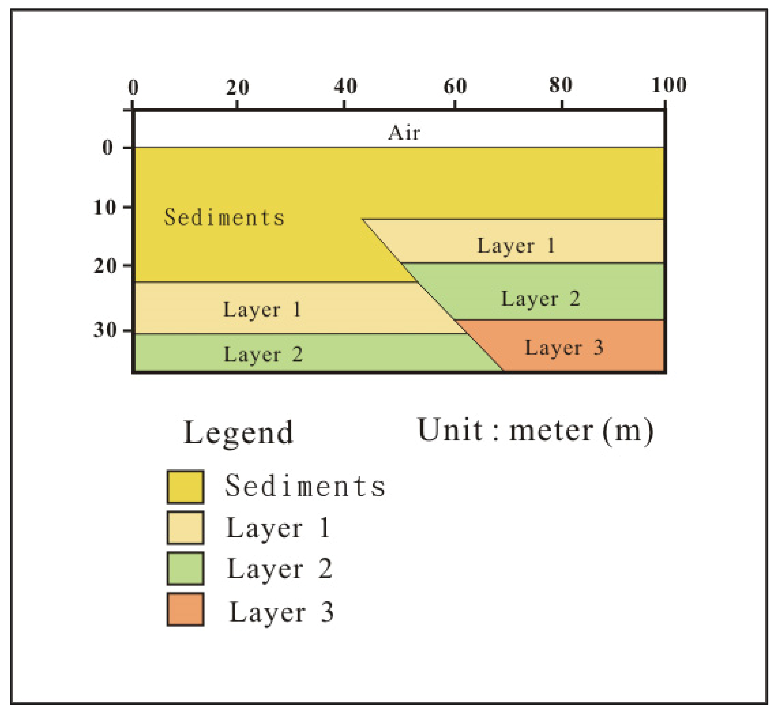
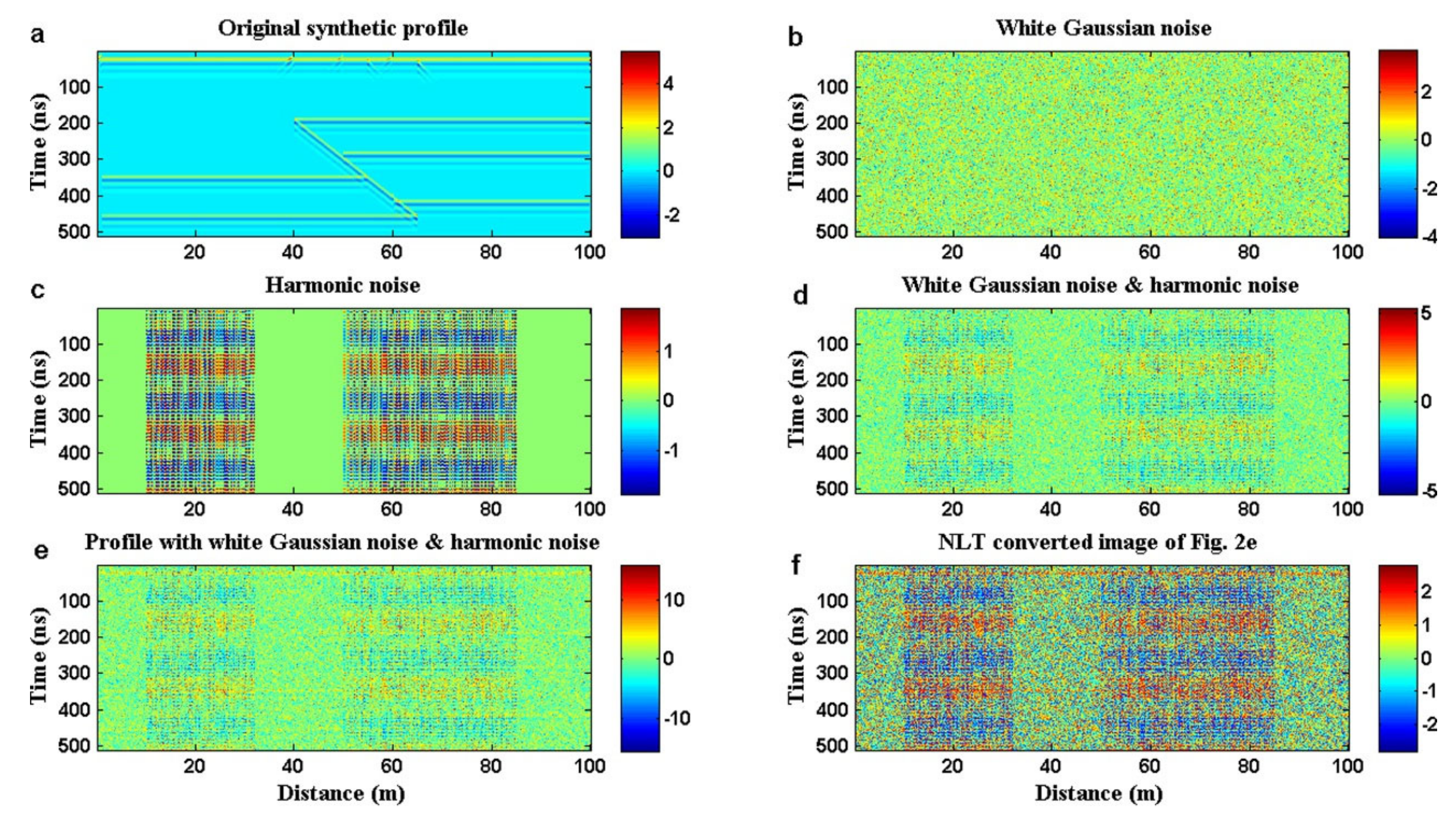
3.1. Hypothetical Model

Figure 1 shows a hypothetical model used for simulating the GPR reflection profile over a subsurface thrust fault structure.

We first simulate an original GPR reflection profile of the thrust fault model in the t-x domain (Figure 2a). This profile is constructed by imitating a common-offset GPR reflection section of a 50 MHz central frequency GPR system. The simulated survey line is 100 m in length with a penetrating depth of about 35 m as indicated in the model (Figure 1). The source pulse simulated is a single zero-phase Ricker wavelet, which is a typical wavelet adopted to produce the synthetic GPR section or seismogram [72]. To circumvent redundant trace editing, the total trace number of the profile is set to 1000 with each trace comprising 1024 samples. Two kinds of noises, namely, the white Gaussian noise (Figure 2b) and harmonic noise (Figure 2c), are used to interfere with the original GPR profile to simulate a noise-corrupted GPR section. Figure 2d demonstrates the combination of the two noises to be added to the original profile. Figure 2e is the outcome of adding the noises shown in Figure 2d to the original profile. As it has been found in previous studies [72,73], the natural logarithmic transform (NLT) is useful in solving the problem of dynamic range in an image; we therefore apply this technique in this study to examine the NLT effect on edge detection. Figure 2f shows the NLT conversion of Figure 2e.

Note that the SNR used for the simulation is 1:3 in amplitude, or –10 dB on the logarithmic dB scale. Obviously, the reflection signal is completely masked by the two added noises.

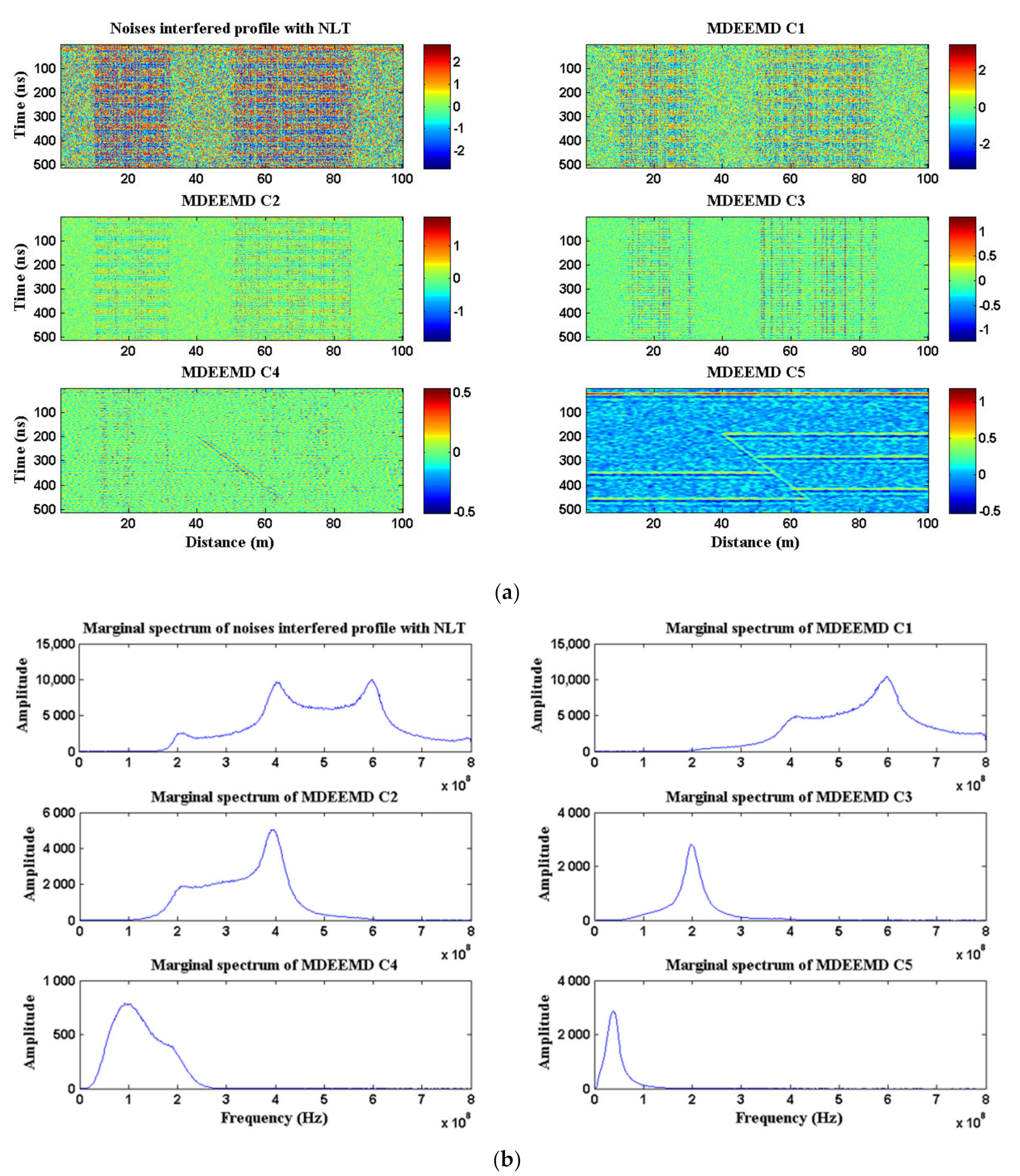
3.1.1. MDEEMD Processing

Once the noise-corrupted profile is obtained, we carry out the MDEEMD process with the standard deviation set to 0.3 for the sifting and 30 for the number of the ensemble members when taking the ensemble mean. Here, only the NLT converted profile (Figure 2f) is used for demonstration because there is no significant difference between the results with and without NLT conversion in this model study. Since the model data are relatively simpler than ordinary GPR reflection data, the IMF profiles are regularized to 5 when employing the most significant components regulation.

Figure 3a demonstrates the MDEEMD result where components C1 to C4 are mainly noise while component C5 contains a significant reflection signal with residues. In other words, component C5 may stand for the combination of the signal and several tail components because the decomposition could be performed further to gain six or even more components. In reality, increasing the number of IMF components without a constraint may be meaningless because it would boost the computation cost considerably, but the improvement of SNR is limited. Figure 3b shows marginal spectra of the noise-corrupted profile and each IMF component for comparison. Obviously, the energy of the marginal spectrum of component C5 is concentrated around 50 MHz with a bandwidth between 25 and 75 MHz, which matches the signal spectrum of the 50 MHz GPR system [59].

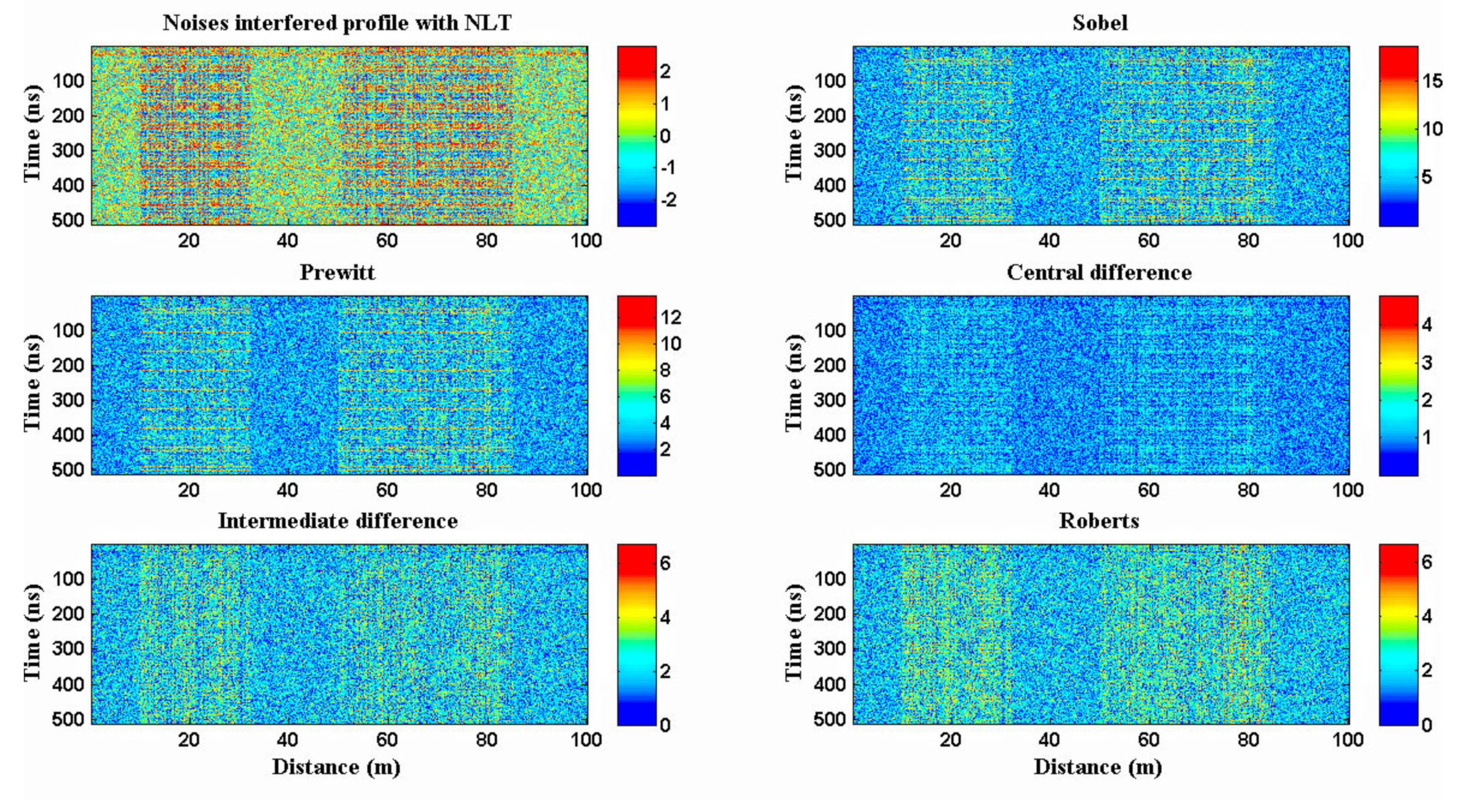
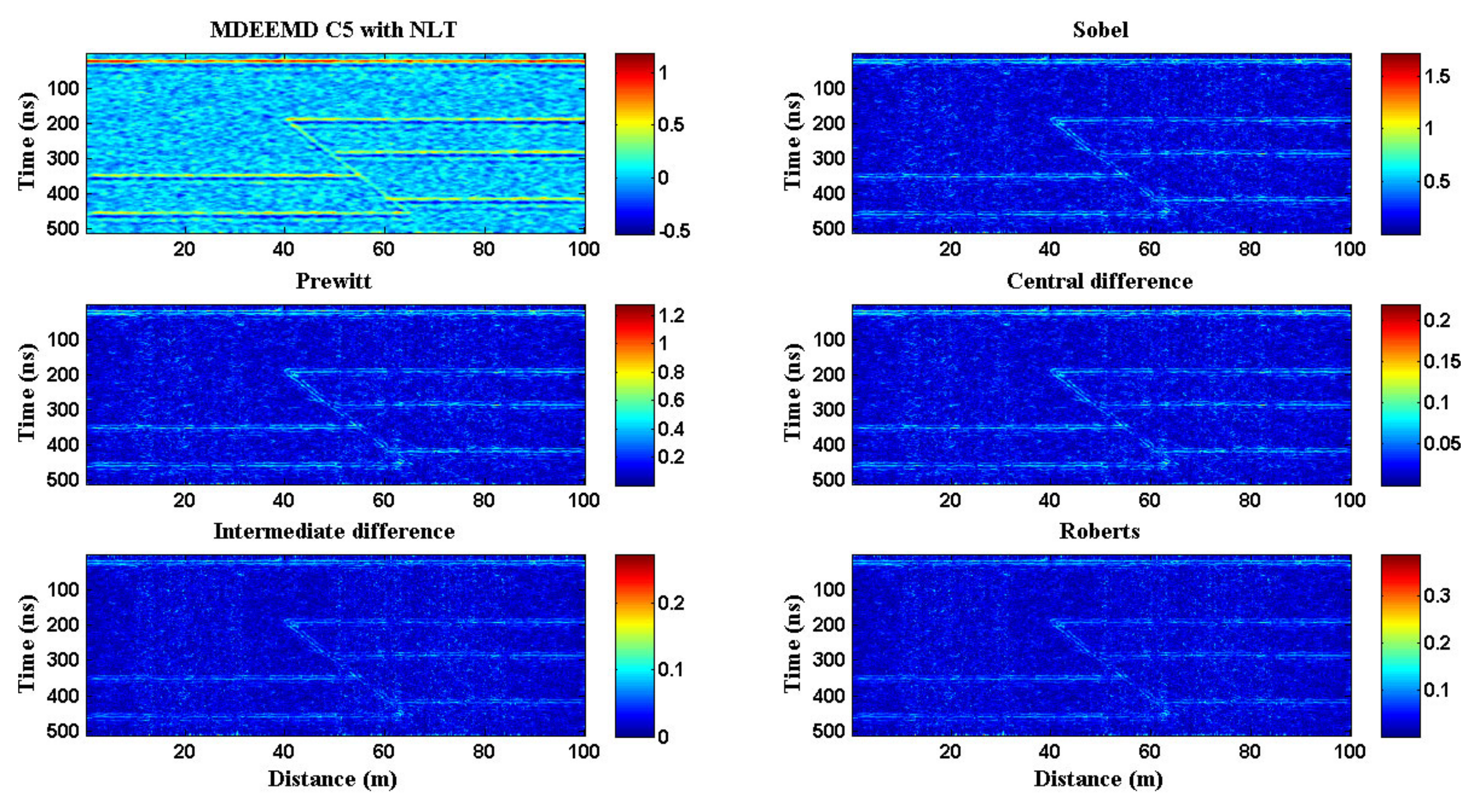
3.1.2. Edge Detecting

The next step is to try the edge detector on the noise-corrupted profile and compare the results with and without the MDEEMD data reconstruction. Figure 4 shows the outcomes of applying five different edge detectors to the noise-corrupted profile without the MDEEMD processing; there is no useful information outlined by each edge detector. In contrast, the thrust structure is highlighted by each edge detector (Figure 5) as we applied MDEEMD to reconstruct the data before carrying out the edge detection.

The edge detectors implemented in the modeling are two-dimensional algorithms which compute the image derivative with respect to the x-axis and y-axis. The gradient magnitude and direction are then obtained from these two vectorized orthogonal components. The direction of this resultant vector is defined as the directional gradient, indicating the direction where the most rapid change occurred. In addition, the magnitude of this resultant vector is called the rapidity of the image in the most rapid changing direction. Here, we use the Sobel detector as an example to illustrate the algorithm. Simply speaking, we calculate approximations of the horizontal and vertical derivatives of the original image by using the x-direction Sobel mask (filter) and y-direction Sobel mask (filter), respectively, then find the gradient of each point in the image by taking the square-root of the sum of the two derivatives. Of course, some researchers may prefer to show the horizontal derivative and the vertical derivatives separately to highlight specific features of the image.

A parallel detecting algorithm is employed to find edges in the intensity of the image and returns a binary edge map constituted by ones where edges are found and zeros elsewhere. This binary edge algorithm searches for places in the image where the intensity changes rapidly, but the most rapid change is not necessary. Depending on the derivative estimator applied, the user may specify the sensitive direction (horizontal, vertical, or both) of the derivatives when determining edges in an image. Since we have no preferred direction, both horizontal and vertical directions are considered in the binary edge algorithm. The two-dimensional algorithm and the binary edge algorithm, each one has its own advantages and disadvantages. The two-dimensional algorithm yields the map of the most rapid change, which enhances the edges but may miss trivial edges. On the other hand, the binary edge map is easier to implement and shows more edges; however, it may look muddled visually and may present fake edges. We make a comparison of these two algorithms in the later field example.

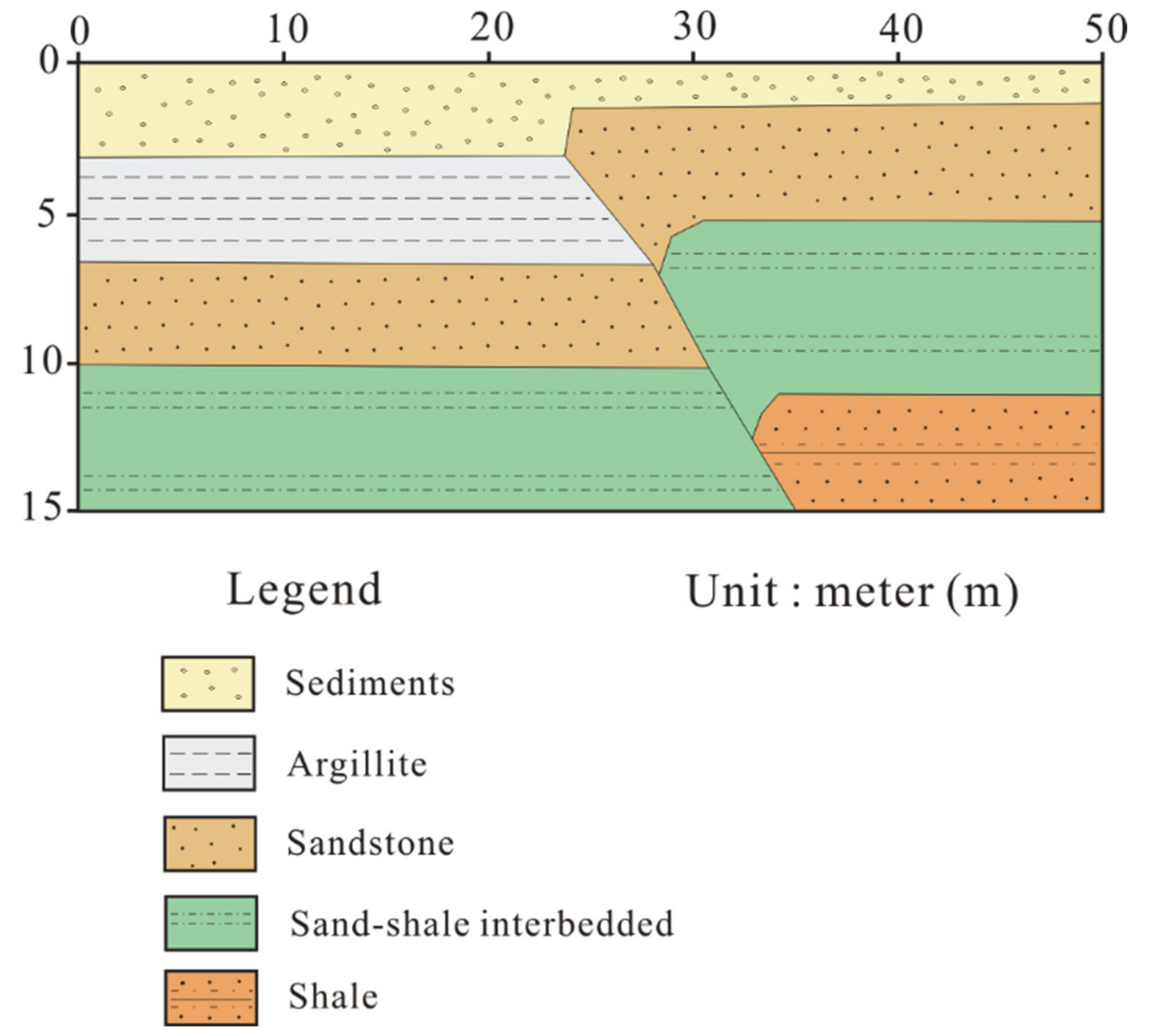
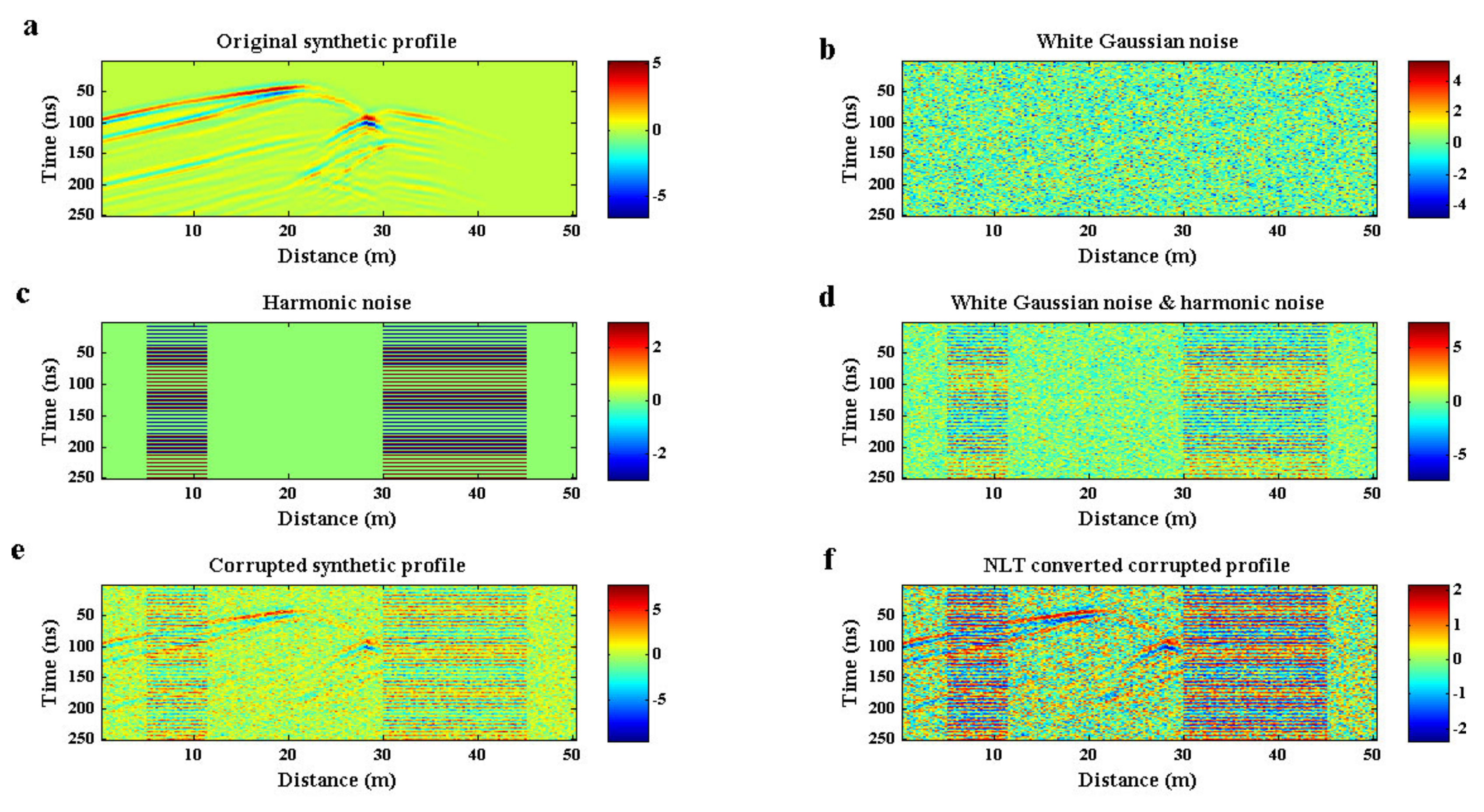
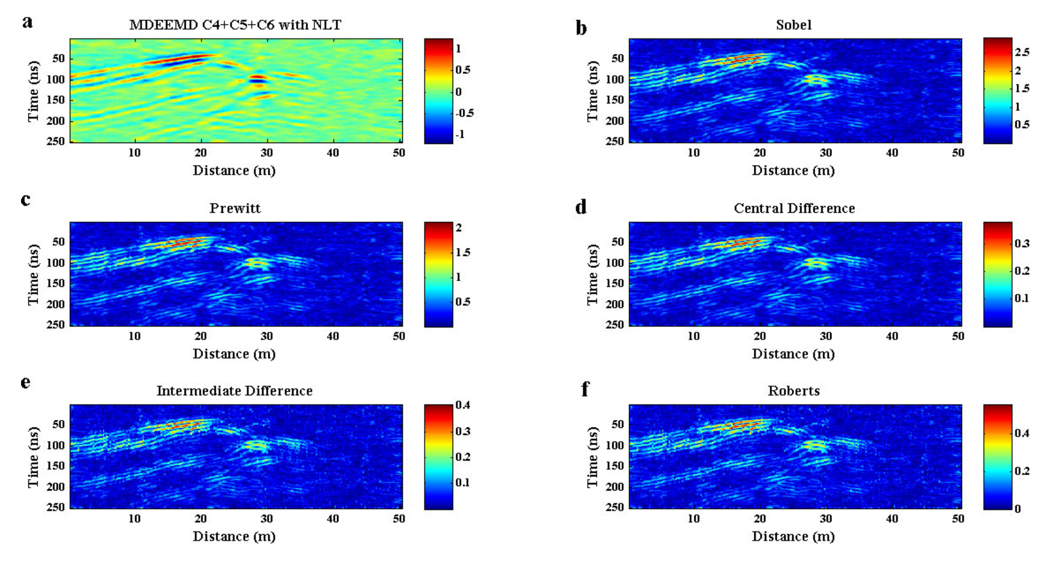
3.2. Realistic Model

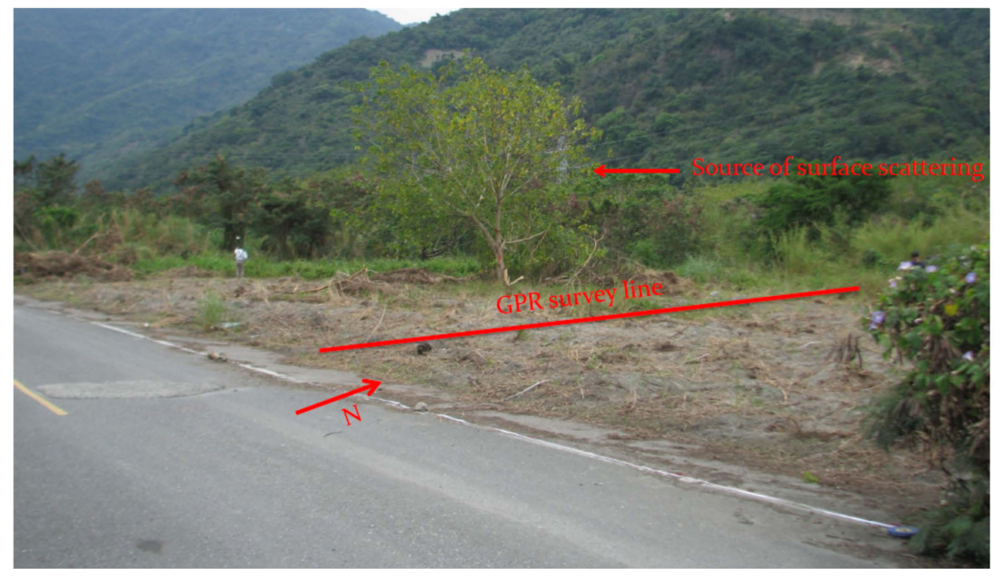
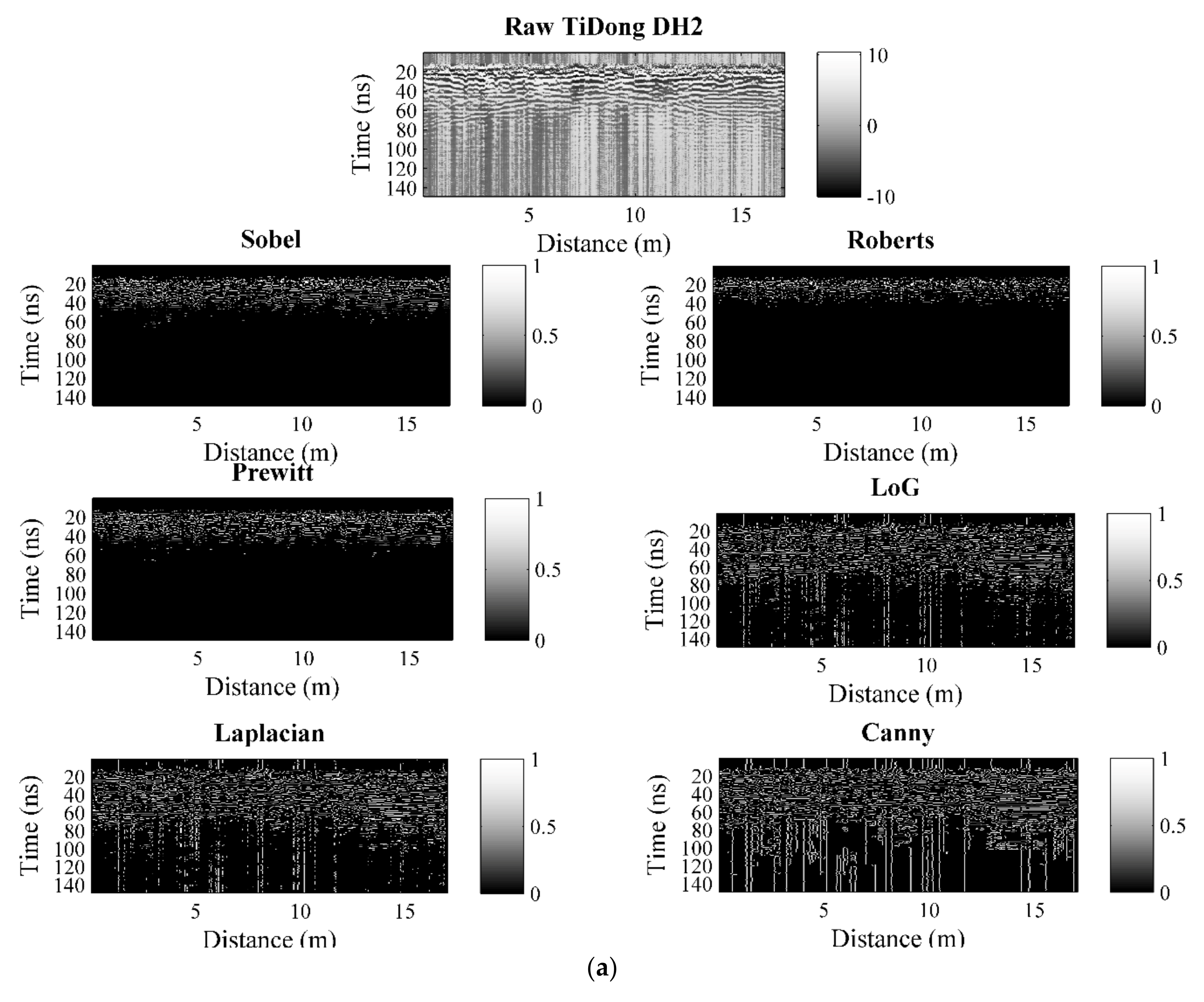
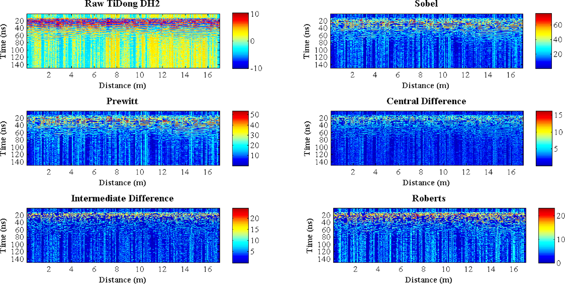
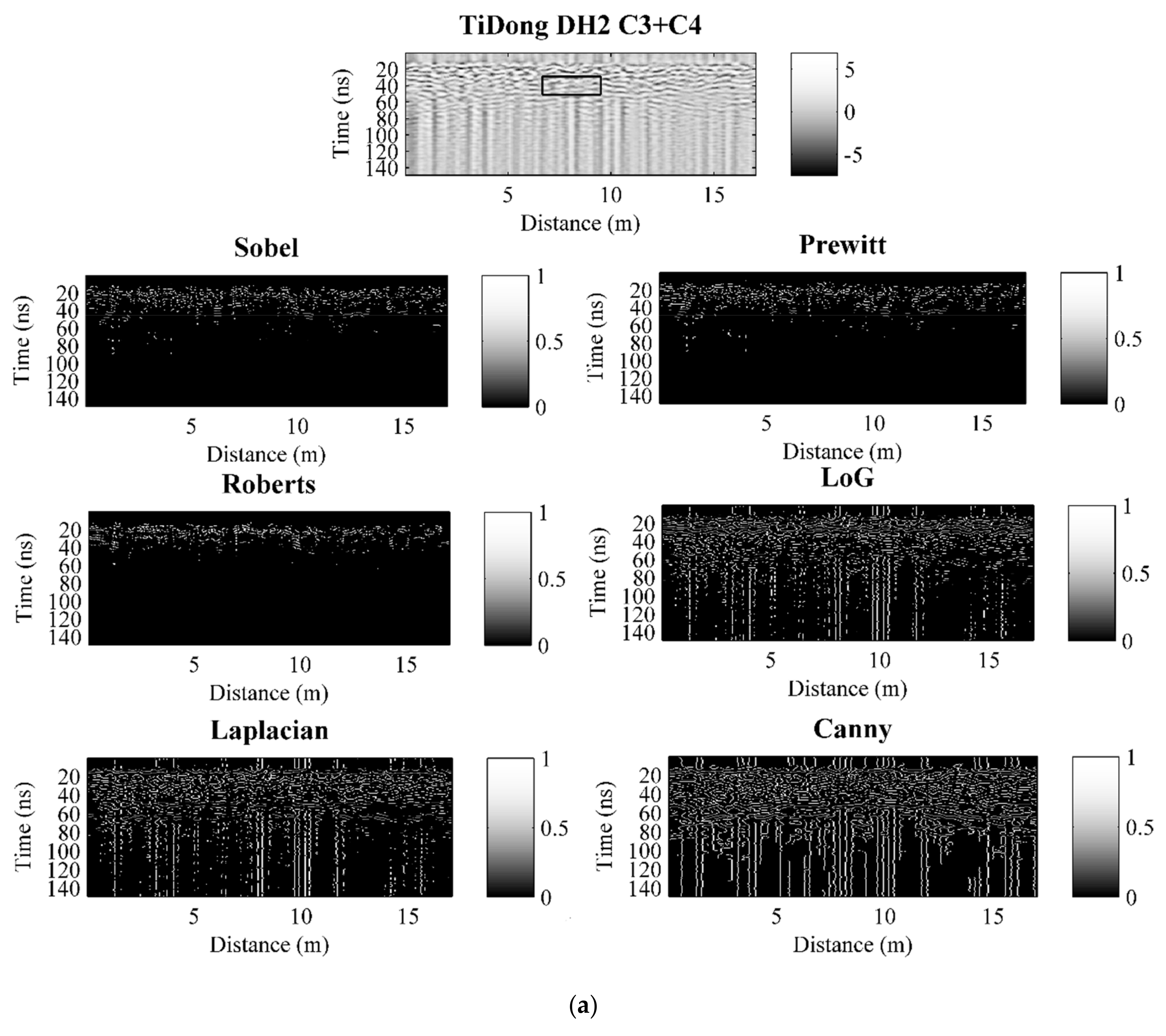
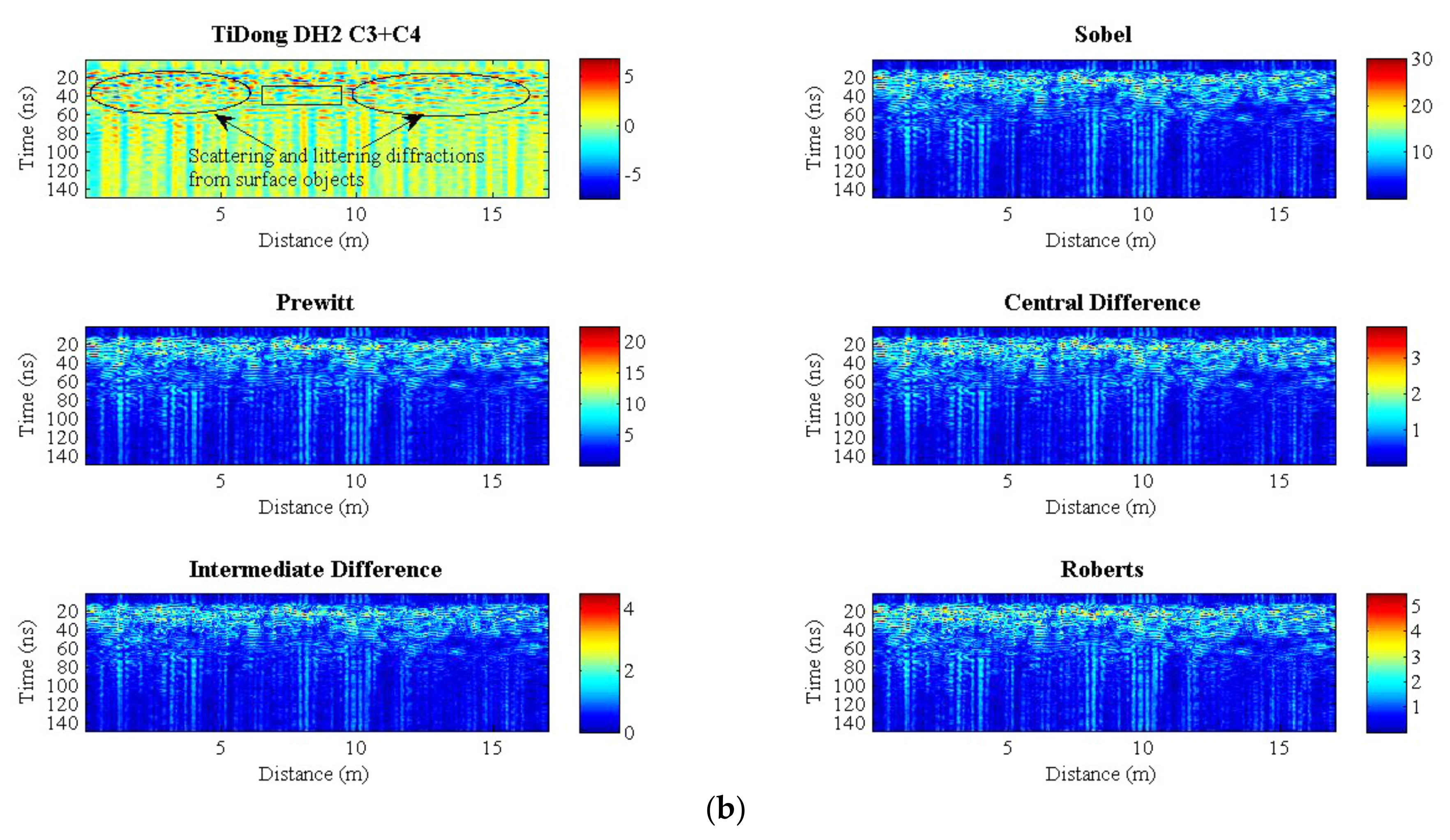
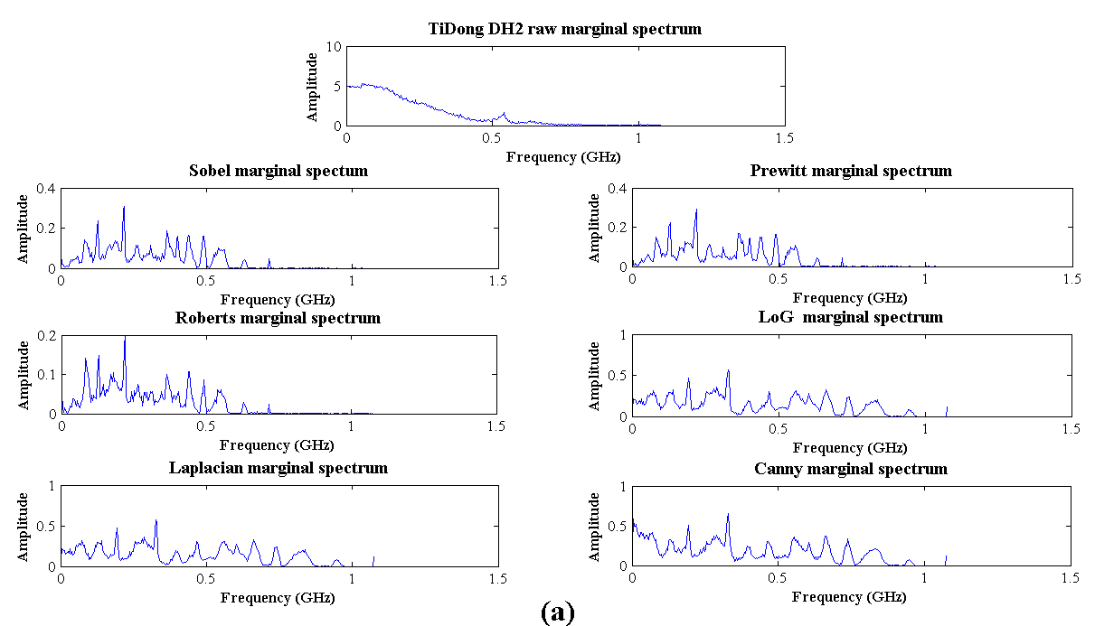
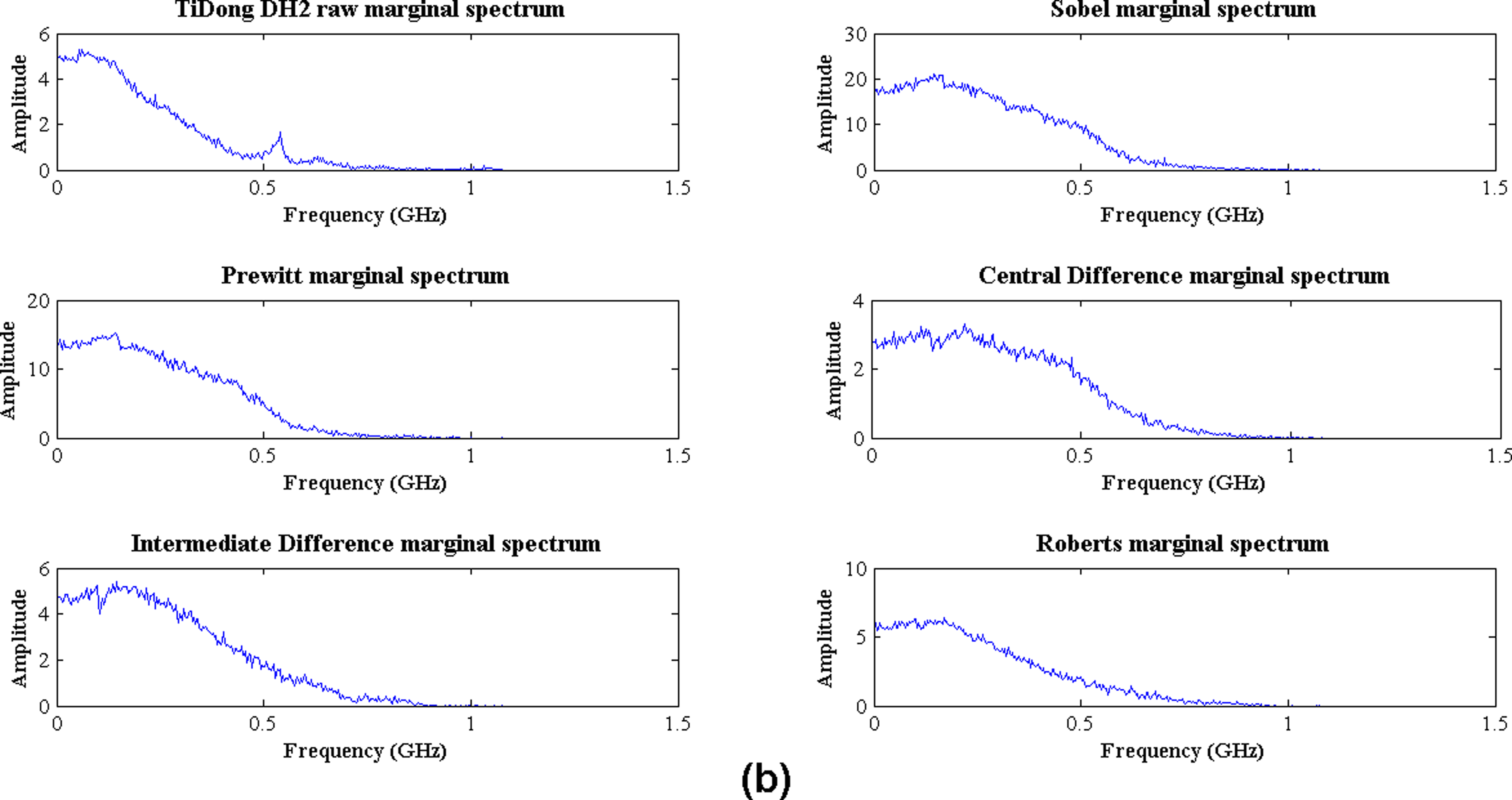
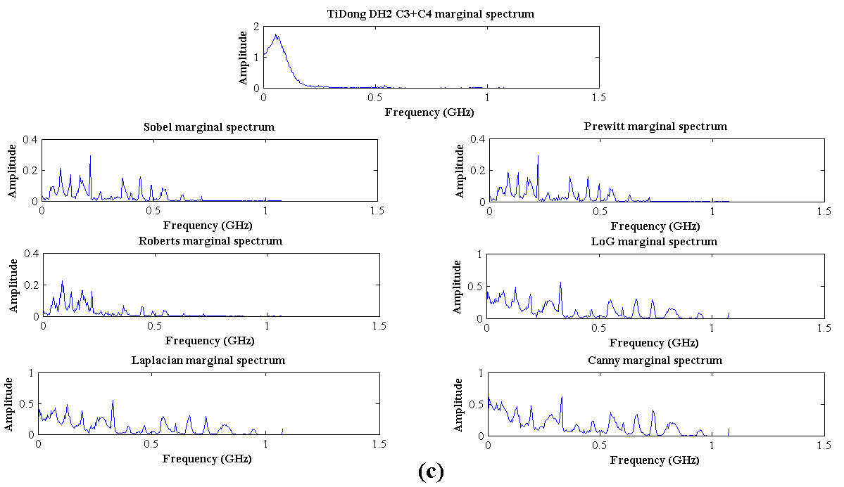
A realistic model is provided along with the simple hypothetical model for comparison. Because the process is the same as in the simple model, we just show the sketch of the realistic model (Figure 6) with the final processed results (Figure 7 and Figure 8). The standard physical parameters (the dielectric permittivity, magnetic permeability, and electrical conductivity) of sediments, argillite, shale, etc. were applied to the realistic model.

In the finite-difference (FD) model simulation, we set an exponential absorbing range for the model boundaries, the Ricker wavelet for the signal type, and 50 MHz for the GPR frequency. The GPR (electromagnetic) simulation is based on the solution of the Maxwell equations. By doing so, it is assumed that the physical parameters are frequency independent and that the physical parameters are constant in y (the depth) direction. The velocities are derived from the standard physical parameters of the geological layers constructed in the model. The spherical spreading factor is already embedded in the raster increments. To solve the problem of the reflections from the boundaries, we adopted an exponential absorbing range for the model boundaries.

3.3. Field Data

To evaluate the feasibility and efficacy of the proposed methodology on a practical application, the processing scheme and techniques demonstrated above are applied to field data for edge detection. A MALA ProEx unshielded bistatic GPR system with 200 MHz antennas of 0.6 m transmitter-to-receiver offset was employed in the field for the data acquisition. The survey site is situated in the range of Taiwan’s southeastern central geological province. The outcrops are majorly argillite intercalated with lensoidal sandstone bodies. The casings of the hot spring wells in this area are constructed with concrete walls around and on top of the hot spring pumps. The area of the well roof is about 2 m× 2 m with a metal lid of 0.6 m × 0.6 m covering the manhole. Most of the wells were buried by pebbles, sand, and mud coming from a devastating debris flow caused by Typhoon Morakot in 2009 and subsequent river floodings. The survey was conducted on a site with a suspected buried hot spring well (Figure 9). Standard common mid-point (CMP) data were acquired from 16 survey lines deployed on the site by setting 1026 samples per trace with 0.47 ns vertical sample interval and 0.05 m horizontal trace spacing. The field line length of each GPR section was about 64.2 m containing 1288 traces. To make the data processing effective, the redundant data were removed from field line sections through data editing.

The final datasets ready for processing were trimmed down to less than 30 m in spatial length and about 300 ns in time depth, but the vertical sample intervals and horizontal trace spacing remain the same. The adjustment of time zero and topographic correction of the data are not required because all of the weeds were cleaned up and the uneven ground surface was flattened before the survey. In this example, we pick out one field line section from the aforementioned 16 survey lines as a representative GPR reflection profile. The spatial length was trimmed down further to 18 m and the time depth was about 150 ns to highlight the possible target. The original (or raw) field section (Figure 10) was processed by using simple data editing and amplitude compensation only; no other techniques have been applied. This field section shows strong periodic horizontal events from approximately 20 ns to 40 ns, which are mostly the lateral waves, system noises, and antenna effects [74,75]. Besides, an interesting strong hyperbolic event with littering diffractions across the entire profile between 40 ns and 80 ns (Figure 10) is confusing. Through the velocity analysis and migration test, we learn that the strong hyperbolic event exhibiting an apparent velocity close to the speed of radar waves travelling through air is a result of scattering by adjacent surface objects on the ground or above the survey line [76,77], and the littering diffractions are generated by the scattering objects within the covered debris [59]. By a simple geometric analysis, we also find that the surface scattering object is a tree near the survey line (Figure 9).

Because the site was disturbed badly when drilling and constructing the hot spring well, the shallow geological structure is fractured and fragmentary. The disturbed landscape and surface scattering result in poor data quality, such that the raw profile does not show distinct layer reflections due to the structural complexity. A more rigorous challenge for the GPR data processing in this case is that the noises arising from rock fragments may degrade the performance of the processing algorithms and the credibility of interpretation.

In order to make an objective comparison, only standard edge detectors (without MDEEMD) were applied to the data at the beginning of the evaluation, as shown in Figure 10, with both binary edge maps (Figure 10a) and two-dimensional edge maps (Figure 10b). At this stage, standard edge detectors are seemingly successful in distinguishing the surface scatterings from reflection events, and those counterfeit events are not highlighted; however, the entire data set is still jumbled. As a result, the complete interpretation of determining the buried object would be difficult under this condition.

The previous model study suggests that if the cluttering of the data was due to low SNR, an improved profile is accessible by integrating the MDEEMD method with edge detection. We therefore tried to carry out the MDEEMD data reconstruction before performing the edge detection. As it has been demonstrated in the model study, the field data were first decomposed by MDEEMD to determine the optimal IMF profiles. With the aid of a marginal spectrum analysis and the physical meaning presented in each IMF profile, we examined the combinations of components 2 and 3, components 2 and 4, and components 3 and 4 for data reconstruction. This trial suggested that the combination of components 3 and 4 was the best. The realization of MDEEMD edge detection is shown in Figure 8. The effect of the MDEEMD approach on spatial resolution can be observed by comparing the profiles shown in Figure 10 and Figure 11. The edge diffractions and cavity ringing of the buried well become more visible as the data were MDEEMD reconstructed (Figure 11). In contrast to Figure 10, the outcomes of edge detecting are greatly improved. To quantitatively verify the results, we provide the marginal spectra, as shown in Figure 12. The frequency range of the GPR system using 200 MHz center frequency antennas is set to between 100 MHz and 300 MHz by the manufacturer. Without the MDEEMD data reconstruction, the dominant frequency band of the acquired GPR data is out of the range even if edge detectors are applied (Figure 12a,b). However, the energy distribution shown in every marginal spectrum of the edge detecting outcomes is greatly improved when using MDEEMD edge detectors (Figure 12c,d).

We also notice that there are no significant signals in the lower half of the time window, however, we still present it to show that the depth factor indeed affects the results even when we have applied the NLT to compensate for the attenuation.

In this case, both the binary and two-dimensional edge maps are presented for comparison. Although the energy concentration in the marginal spectrum of the binary edge maps is not as distinct as that in the two-dimensional edge maps, the improvement is still evident. In fact, the different results of these two algorithms are just a matter of presenting the changes at the boundaries. The binary maps show the places where the intensity changes rapidly, rather than the most rapid change similar to the two-dimensional edge maps. Therefore, the binary edge maps look muddle when compared with the two-dimensional edge maps, and their marginal spectra tend to disperse in a wider range.

The onsite excavation recovered the buried hot spring well (Figure 13); its reflection signal is indicated within the thick rectangular line box shown in Figure 11. Comparing Figure 11a with Figure 11b, we notice that the boundary of the hot spring well is more visible on the two-dimensional edge maps than the binary edge maps.

4. Discussion

As mentioned previously in this paper, noise suppression is essential in edge detection. Some advanced edge detectors are implemented by using Fourier-based filters, a Gaussian filter, for instance, to convolve with the data for noise suppression before applying the edge detection. The Fourier method is commonly used in digital signal processing, but special attention should be drawn to its adverse effects because the convolution in the filtering procedure may generate unwanted artifacts if spurious signals exist. In contrast, the MDEEMD edge detection is a data-driven multiscale adaptive approach that is not limited by the uncertainty principle and does not need spurious harmonics and negative frequency in analyzing the data; the difficulties caused by Fourier-based filters can be circumvented as a result. However, it could be an interesting argument regarding the sophisticated techniques involved in the MDEEMD edge detection. Chen and Jeng [45] investigated a nearby survey line of longer length and shallower depth range, processed by using only the MDEEMD algorithm with different reconstruction strategies. The achievement of their primitive method was encouraging, but the target boundaries were still an issue. Jeng et al. [78] proposed a brief idea of the GPR MDEEMD edge detection in a conference abstract lacking a quantitative analysis and processing details. In this study, we assimilate all of the renovating techniques and exploit the marginal spectrum analysis to quantify the data reconstruction such that we can make a more accurate interpretation. We understand that the complexity of the MDEEMD edge detectors could be a hurdle that prohibits their widespread use. Some investigators may prefer a compact scheme in GPR data processing; however, an advanced methodology is still necessary when processing low SNR data. Conversely, high-quality data may not need the proposed technique, but considerable labor and better GPR instrumentation in the field data acquisition are the tradeoffs. The integration of MDEEMD and edge detectors into GPR data processing indicates that the target signal within a complicated dataset can be retrieved more efficiently than using either one method alone. Thus, a practical compromise should be worked out between the survey endeavor and data processing complexity.

As noted in the literature, the edge detecting output of an image is not a real image any longer because the amount of data representing the original image may be reduced greatly and the features that are regarded as less relevant are discarded [37,79]. Consequently, only the important components determined by the algorithm remain. The advantages of applying edge detectors are enhancing the target boundaries, avoiding the subsequent complicated data processing, and simplifying the image interpretation. Although the GPR profile is similar to an image, and we did process it as an image, the GPR profile is not a real image, actually. Therefore, the image-like appearance is not important. What we are interested in is to compactly map the target within the acquired reflection data. Thus, the use of simple one-dimensional boundary lines and curves to indicate the image information should be desirable.

In the field example, there are no drill data available, so we just present the timescale which is more objective. In fact, we could estimate the root-mean-squared (RMS) velocity function by examining diffraction hyperbolas or common mid-point (CMP) data, but the results were doubtful due to the interference from the troublesome top debris layer.

It must also be mentioned that the proposed technique may not be ready for the color edge detection algorithm, which is one of the major topics in edge detection; however, the multidimensional decomposition and data reconstruction of the MDEEMD approach will at least shed some light on the color edge detection algorithm [80].

5. Conclusions

We have shown that the use of the MDEEMD data reconstruction technique can greatly improve the result of edge detecting in the target mapping of GPR data of a buried hot spring well survey. MDEEMD is a data-driven nonlinear and nonstationary multidimensional data processing method that has been successfully applied to various fields of study before we applied it to the investigation of a buried water utility infrastructure. For data acquired from complicated sites, MDEEMD can improve edge detection in delineating target structures. If the performance of the edge detection is degraded by noises, MDEEMD provides a solution to boost the SNR, and thus the fake response can be minimized. Although numerous data procession methods are available for SNR enhancement, the MDEEMD algorithm offers a better solution by circumventing the difficulties originating from the Fourier theory which is widely assumed in most data processing methods.

Although this study is focused on applying the MDEEMD edge detection to GPR data of a buried hot spring well, we believe that this novel technique should not be limited to this case. It could be extended to process other kinds of water resources and management data, seismic reflection data in particular, because the seismic data format is similar to GPR in general. Besides, since we treat each data point of the GPR profile as an image pixel, the proposed method is applicable to common image processing with limited modification.

References

1. Jaw, S.W.; Hashim, M. Locational accuracy of underground utility mapping using ground penetrating radar. Tunn. Undergr. Sp. Technol. 2013, 35, 20–29. [Google Scholar] [CrossRef]
2. Bernatek-Jakiel, A.; Kondracka, M. Combining geomorphological mapping and near surface geophysics (GPR and ERT) to study piping systems. Geomorphology 2016, 274, 193–209. [Google Scholar] [CrossRef]
3. Forte, E.; Pipan, M. Review of multi-offset GPR applications: Data acquisition, processing and analysis. Signal Process. 2017, 132, 210–220. [Google Scholar] [CrossRef]
4. Lai, W.W.L.; Dérobert, X.; Annan, P. A review of Ground Penetrating Radar application in civil engineering: A 30-year journey from Locating and Testing to Imaging and Diagnosis. NDT E Int. 2018, 96, 58–78. [Google Scholar]
5. Park, B.; Kim, J.; Lee, J.; Kang, M.-S.; An, Y.-K. Underground object classification for urban roads using instantaneous phase analysis of Ground-penetrating radar (GPR) data. Remote Sens. 2018, 10, 1417. [Google Scholar] [CrossRef] [Green Version]
6. Got, J.B.; Bielders, C.; Lambot, S. Characterizing soil piping networks in loess-derived soils using ground-penetrating radar. In Geophysical Research Abstracts; EGU General Assembly: Vienna, Austria, 2019; p. 7038. [Google Scholar]
7. Garcia-Lamont, F.; Cervantes, J.; López, A.; Rodriguez, L. Segmentation of images by color features: A survey. Neurocomputing 2018, 292, 1–27. [Google Scholar] [CrossRef]
8. Yaacob, R.; Ooi, C.D.; Ibrahim, H.; Hassan, N.F.N.; Othman, P.J.; Hadi, H. Automatic extraction of two regions of creases from palm print images for biometric identification. J. Sens. 2019, 2019, 1–12. [Google Scholar] [CrossRef]
9. Tariq, N.; Hamzah, R.A.; Ng, T.F.; Wang, S.L.; Ibrahim, H. Quality assessment methods to evaluate the performance of edge detection algorithms for digital image: A systematic literature review. IEEE Access 2021, 9, 87763–87776. [Google Scholar] [CrossRef]
10. Davis, L.S. A survey of edge detection techniques. Comput. Graph. Image Process. 1975, 4, 248–270. [Google Scholar] [CrossRef]
11. Nevatia, R. A color edge detector and its use in scene segmentation. IEEE Trans. Syst. Man. Cybern. 1977, 7, 820–826. [Google Scholar] [CrossRef]
12. Nabighian, M.N. The analytic signal of two-dimensional magnetic bodies with polygonal cross-section: Its properties and use for automated anomaly interpretation. Geophysics 1972, 37, 507–517. [Google Scholar] [CrossRef]
13. Roest, W.R.; Verhoef, J.; Pilkington, M. Magnetic interpretation using the 3-D analytic signal. Geophysics 1992, 57, 116–125. [Google Scholar] [CrossRef]
14. Hsu, S.K.; Sibuet, J.C.; Shyu, C.T. High-resolution detection of geologic boundaries from potential-field anomalies: An enhanced analytic signal technique. Geophysics 1996, 61, 373–386. [Google Scholar] [CrossRef]
15. Tabbagh, M.; Desvignes, A.; Dabas, G. Processing of Z gradiometer magnetic data using linear transforms and analytical signal. Archaeol. Prospect. 1997, 4, 1–13. [Google Scholar] [CrossRef]
16. Jeng, Y.; Lee, Y.L.; Chen, C.Y.; Lin, M.J. Integrated signal enhancements in magnetic investigation in archaeology. J. Appl. Geophys. 2003, 53, 31–48. [Google Scholar] [CrossRef]
17. Du, W.; Wu, Y.; Guan, Y.; Hao, M. Edge detection in potential filed using the correlation coefficients between the average and standard deviation of vertical derivatives. J. Appl. Geophys. 2017, 143, 231–238. [Google Scholar] [CrossRef]
18. Cooper, G.R.J.; Cowan, D.R. Edge enhancement of potential-field data using normalized statistics. Geophysics 2008, 73, H1–H4. [Google Scholar] [CrossRef]
19. Ma, G.; Li, L. Edge detection in potential fields with the normalized total horizontal derivative. Comput. Geosci. 2012, 41, 83–87. [Google Scholar] [CrossRef]
20. Ma, G.; Liu, C.; Li, L. Balanced horizontal derivative of potential field data to recognize the edges and estimate location parameters of the source. J. Appl. Geophys. 2014, 108, 12–18. [Google Scholar] [CrossRef]
21. Zhu, Y.; Wang, W.; Farquharson, C.; Huang, J.; Zhang, M.; Yang, M.; Wang, D. Normalized vertical derivatives in the edge enhancement of maximum-edge-recognition methods in potential fields. Geophysics 2021, 4, G23–G34. [Google Scholar] [CrossRef]
22. Blakely, R.J.; Simpson, R.W. Approximating edges of source bodies from magnetic or gravity anomalies. Geophysics 1986, 51, 1494–1498. [Google Scholar] [CrossRef]
23. Oruç, B.; Sertçelik, I.; Kafadar, Ö.; Selim, H.H. Structural interpretation of the Erzurum Basin, eastern Turkey, using curvature gravity gradient tensor and gravity inversion of basement relief. J. Appl. Geophys. 2013, 88, 105–113. [Google Scholar] [CrossRef]
24. Chen, L.; Tsang, I.W.; Xu, D. Laplacian embedded regression for scalable manifold regularization. IEEE Trans. Neural Netw. Learn. Syst. 2012, 23, 902–915. [Google Scholar] [CrossRef]
25. Shrivakshan, G.T.; Chandrasekar, C. A Comparison of various Edge Detection Techniques used in Image Processing. Int. J. Comput. Sci. 2012, 9, 269–276. [Google Scholar]
26. Silva, P.M.; Martins, L.; Pampanelli, P.; Faustino, G. Why curvature attribute delineates subtle geologic features? A mathematical approach. Expanded Abstract. In Proceedings of the 86th SEG Annual Meeting, Dallas, TX, USA, 16 October 2016; pp. 1913–1918. [Google Scholar] [CrossRef]
27. Miller, H.G.; Singh, V. Potential field tilt—a new concept for location of potential field sources. J. Appl. Geophys. 1994, 32, 213–217. [Google Scholar] [CrossRef]
28. Aydin, T.; Yemez, Y.; Anarim, E.; Sankur, B. Multidirectional and multiscale edge detection via M-band wavelet transform. IEEE Trans. Image Process. 1996, 5, 1370–1377. [Google Scholar] [CrossRef]
29. Boustani, B.; Javaherian, A.; Nabi-Bidhendi, M.; Torabi, S.; Amindavar, H.R. Mapping channel edges in seismic data using curvelet transform and morphological filter. J. Appl. Geophys. 2019, 160, 57–68. [Google Scholar] [CrossRef]
30. Jeng, Y.; Lin, C.H.; Li, Y.W.; Chen, C.S.; Yu, H.M. Application of sub-image multiresolution analysis of Ground-penetrating radar data in a study of shallow structures. J. Appl. Geophys. 2011, 73, 251–260. [Google Scholar] [CrossRef]
31. Turiel, A.; DelPozo, A. Reconstructing images from their most singular fractal manifold. IEEE Trans. Image Process. 2002, 11, 345–350. [Google Scholar] [CrossRef]
32. Maji, S.K.; Yahia, H.M.; Badri, H. Reconstructing an image from its edge representation. Digit. Signal Process. 2013, 23, 1867–1876. [Google Scholar] [CrossRef] [Green Version]
33. Wang, J.; Meng, X.; Li, F. Improved curvature gravity gradient tensor with principal component analysis and its application in edge detection of gravity data. J. Appl. Geophys. 2015, 118, 106–114. [Google Scholar] [CrossRef]
34. Yuan, Y.; Huang, D.; Yu, Q.; Lu, P. Edge detection of potential field data with improved structure tensor methods. J. Appl. Geophys. 2014, 108, 35–42. [Google Scholar] [CrossRef]
35. Ma, G.; Liu, C.; Huang, D. The removal of additional edges in the edge detection of potential field data. J. Appl. Geophys. 2015, 114, 168–173. [Google Scholar] [CrossRef]
36. Pilkington, M.; Tschirhart, V. Practical considerations in the use of edge detectors for geologic mapping using magnetic data. Geophysics 2017, 82, J1–J8. [Google Scholar] [CrossRef]
37. Cooper, G.R.J. The removal of unwanted edge contours from gravity datasets. Explor. Geophys. 2013, 44, 42–47. [Google Scholar] [CrossRef]
38. Cooper, G.R.J. Reducing the dependence of the analytic signal amplitude of aeromagnetic data on the source vector direction. Geophysics 2014, 79, J55–J60. [Google Scholar] [CrossRef]
39. Manzi, M.S.D.; Durrheim, R.J.; Hein, K.A.A.; King, N. 3D edge detection seismic attributes used to map potential conduits for water and methane in deep gold mines in the Witwatersrand basin. South Africa. Geophysics 2012, 77, WC133–WC147. [Google Scholar] [CrossRef]
40. Ashraf, H.; Mousa, W.A.; AlDossary, S. Sobel filter for edge detection of hexagonally sampled 3D seismic data. Geophysics 2016, 81, N41–N51. [Google Scholar] [CrossRef]
41. Zheng, J.; Peng, S.P.; Yang, F. A novel edge detection for buried target extraction after SVD-2D wavelet processing. J. Appl. Geophys. 2014, 106, 106–113. [Google Scholar] [CrossRef]
42. Belina, F.A.; Dafflon, B.; Tronicke, J.; Holliger, K. Enhancing the vertical resolution of surface georadar data. J. Appl. Geophys. 2009, 68, 26–35. [Google Scholar] [CrossRef]
43. Nielsen, L.; Møller, I.; H.Nielsen, L.; Johannessen, P.N.; Pejrup, M.; Andersen, T.J.; Korshøj, J.S. Integrating ground-penetrating radar and borehole data from a Wadden Sea barrier island. J. Appl. Geophys. 2009, 68, 47–59. [Google Scholar] [CrossRef]
44. Tzanis, A. A versatile tuneable curvelet-like directional filter with application to fracture detection in two-dimensional GPR data. Signal Process. 2017, 132, 243–260. [Google Scholar] [CrossRef]
45. Chen, C.S.; Jeng, Y. A data-driven multidimensional signal-noise decomposition approach for GPR data processing. Comput. Geosci. 2015, 85, 164–174. [Google Scholar] [CrossRef]
46. Roberts, L.G. Machine Perception of Three-Dimensional Solids. Ph.D. Thesis, Massachusetts Institute of Technology, Cambridge, MA, USA, 1963. [Google Scholar]
47. Sobel, G.; Feldman, I. A 3 × 3 Isotropic Gradient Operator for Image Processing. In Pattern Classification and Scene Analysis; Academic Press: New York, NY, USA, 1968. [Google Scholar]
48. Prewitt, J. Object enhancement and extraction. In Picture Processing and Psychopictorics; Academic Press: New York, NY, USA, 1970. [Google Scholar]
49. Canny, J. A Computational Approach to Edge Detection. IEEE Trans. Pattern Anal. Mach. Intell. 1986, 6, 679–698. [Google Scholar] [CrossRef]
50. Green, B. Canny Edge Detection Tutorial. 2002. Available online: https://web.archive.org/web/20160324173252/http://dasl.mem.drexel.edu/alumni/bGreen/www.pages.drexel.edu/_weg22/can_tut.html (accessed on 25 July 2021).
51. Accame, M.; DeNatale, F.G.B. Edge detection by point classification of Canny filtered images. Signal Processing 1997, 60, 11–22. [Google Scholar] [CrossRef]
52. Marr, D. Vision: A Computational Investigation into the Human Representation and Processing of Visual Information; W. H. Freeman and Company: San Francisco, CA, USA, 1982; pp. 54–78. [Google Scholar]
53. Lindeberg, T. Scale-Space Theory in Computer Vision; Springer: Berlin/Heidelberg, Germany, 1994. [Google Scholar]
54. Ma, G.; Huang, D.; Meng, L. Improved structure tensor in the edge detection of potential field data. WIT Trans. Ecol. Environ. 2014, 189, 563–569. [Google Scholar] [CrossRef]
55. Huang, N.E.; Shen, Z.; Long, S.R.; Wu, M.C.; Snin, H.H.; Zheng, Q.; Yen, N.C.; Tung, C.C.; Liu, H.H. The empirical mode decomposition and the Hubert spectrum for nonlinear and non-stationary time series analysis. Proc. R. Soc. A Math. Phys. Eng. Sci. 1998, 454, 903–995. [Google Scholar] [CrossRef]
56. Chen, C.S.; Jeng, Y. Two-dimensional nonlinear geophysical data filtering using the multidimensional EEMD method. J. Appl. Geophys. 2014, 111, 256–270. [Google Scholar] [CrossRef] [Green Version]
57. Wu, Z.H.; Huang, N.E.; Chen, X.Y. The multi-dimensional ensemble empirical mode decomposition method. Adv. Adapt. Data Anal. 2009, 1, 339–372. [Google Scholar] [CrossRef]
58. Tzanis, A. Detection and extraction of orientation-and-scale-dependent information from two-dimensional GPR data with tuneable directional wavelet filters. J. Appl. Geophys. 2013, 8, 48–67. [Google Scholar] [CrossRef]
59. Chen, C.S.; Jeng, Y. GPR investigation of the near-surface geology in a geothermal river valley using contemporary data decomposition techniques with forward simulation modeling. Geothermics 2016, 64, 439–454. [Google Scholar] [CrossRef]
60. Huang, N.E.; Wu, Z. a Review on Hilbert-Huang Transform: Method and Its Applications. Rev. Geophys. 2008, 46, 1–23. [Google Scholar] [CrossRef] [Green Version]
61. Flandrin, P.; Rilling, G.; Goncalves, P. Empirical mode decomposition as a filter bank. IEEE Signal Process. Lett. 2004, 11, 112–114. [Google Scholar] [CrossRef] [Green Version]
62. Wu, Z.H.; Huang, N.E. Ensemble empirical mode decomposition: A noise-assisted data analysis method. Adv. Adapt. Data Anal. 2009, 1, 1–41. [Google Scholar] [CrossRef]
63. Huang, N.E.; Shen, Z.; Long, S.R. A new view of nonlinear water waves: The Hilbert spectrum. Annu. Rev. Fluid Mech. 1999, 31, 417–457. [Google Scholar] [CrossRef] [Green Version]
64. Lozano, M.; Fiz, J.A.; Jané, R. Performance evaluation of the Hilbert-Huang transform for respiratory sound analysis and its application to continuous adventitious sound characterization. Signal Process. 2016, 120, 99–116. [Google Scholar] [CrossRef] [Green Version]
65. Stollnitz, E.J.; DeRose, T.D.; Salestin, D.H. Wavelets for computer graphics: A primer. Part 1. IEEE Comput. Graph. Appl. 1995, 15, 76–84. [Google Scholar] [CrossRef]
66. Tzanis, A. The Curvelet Transform in the analysis of 2-D GPR data: Signal enhancement and extraction of orientation-and-scale-dependent information. J. Appl. Geophys. 2015, 115, 145–170. [Google Scholar] [CrossRef]
67. Liu, Y.; Fomel, S. Seismic data interpolation beyond aliasing using regularized nonstationary autoregression. Geophysics. 2011, 76, V69–V77. [Google Scholar] [CrossRef]
68. Hauser, S.; Ma, J. Seismic Data Reconstruction via Shearlet-Regularized Directional Inpainting. Available online: http://citeseerx.ist.psu.edu/viewdoc/download?doi=10.1.1.572.1557&rep=rep1&type=pdf (accessed on 30 August 2021).
69. Looney, D.; Mandic, D.P. Multiscale Image Fusion Using Complex Extensions of EMD. IEEE Trans. Signal Process. 2009, 57, 1626–1630. [Google Scholar] [CrossRef]
70. Jeng, Y.; Lin, M.J.; Chen, C.S.; Wang, Y.H. Using a Nonlinear Decomposition Method. Geophysics 2007, 72, F223–F235. [Google Scholar] [CrossRef]
71. Chen, C.S.; Chien, T.S.; Lee, P.L.; Jeng, Y.; Yeh, T.K. Prefrontal Brain Electrical Activity and Cognitive Load Analysis Using a Non-linear and Non-Stationary Approach. IEEE Access 2020, 8, 211115–211124. [Google Scholar] [CrossRef]
72. Chen, C.S.; Jeng, Y. Natural logarithm transformed EEMD instantaneous attributes of reflection data. J. Appl. Geophys. 2013, 95, 53–65. [Google Scholar] [CrossRef]
73. Jeng, Y.; Chen, C.S. A nonlinear method of removing harmonic noise in geophysical data. Nonlinear. Process. Geophys. 2011, 18, 367–379. [Google Scholar] [CrossRef] [Green Version]
74. Radzevicius, S.J.; Guy, E.D.; Daniels, J.J. Pitfalls in GPR data interpretation: Differentiating stratigraphy and buried objects from periodic antenna and target effects. Geophys. Res. Lett. 2000, 27, 3393–3396. [Google Scholar] [CrossRef] [Green Version]
75. Jeng, Y.; Chen, C.S. Subsurface GPR imaging of a potential collapse area in urban environments. Eng. Geol. 2012, 147–148. [Google Scholar] [CrossRef]
76. Sun, J.; Young, R.A. Recognizing surface scattering in ground-penetrating radar data. Geophysics 1995, 60, 1378–1385. [Google Scholar] [CrossRef]
77. Bano, M.; Marquis, G.; Nivière, B.; Maurin, J.C.; Cushing, M. Investigating alluvial and tectonic features with ground penetrating radar and analyzing diffractions patterns. J. Appl. Geophys. 2000, 43, 33–41. [Google Scholar] [CrossRef]
78. Jeng, Y.; Chen, C.S.; Chen, S.C. Multidimensional EMD-based edge detection and the application to GPR imaging. In Proceedings of the EGU General Assembly Conference Abstracts, Vienna, Austria, 23–28 April 2017; p. 1982. [Google Scholar]
79. Lindeberg, T. Edge detection and ridge detection with automatic scale selection. In Proceedings of the CVPR IEEE Computer Society Conference on Computer Vision and Pattern Recognition, San Francisco, CA, USA, 18–20 June 1996; pp. 465–470. [Google Scholar] [CrossRef] [Green Version]
80. Plataniotis, K.N.; Venetsanopoulos, A.N. Color Image Processing and Applications; Springer: Berlin/Heidelberg, Germany, 2000. [Google Scholar] [CrossRef]
Figure 1. Hypothetical model of a thrust fault for the synthetic model study.
Water 13 03148 g001
Figure 2. Synthetic hypothetical model profile, interfering noises, and noise-corrupted profiles. (a) GPR reflection profile of the proposed model. (b) White Gaussian noise. (c) Harmonic noise. (d) Combination of the white Gaussian noise and harmonic noise. (e) GPR reflection profile corrupted by the white Gaussian noise and harmonic noise. (f) NLT conversion of the noise-corrupted reflection profile. The model signal is invisible after noises are added.
Water 13 03148 g002
Figure 3. MDEEMD components and marginal spectra of the hypothetical model. (a) Decomposed components of the noise-corrupted profile shown in Figure 2f. (b) Marginal spectra for comparison.
Water 13 03148 g003
Figure 4. Two-dimensional edge maps of the hypothetical model study using various edge detectors without MDEEMD. Note that in this figure and the following, the central difference and intermediate difference indicate the Canny detector using a finite-difference scheme of central difference scheme and backward difference scheme, respectively.
Water 13 03148 g004
Figure 5. Two-dimensional edge maps of the hypothetical model study with MDEEMD. Various edge detectors are applied to the noise-corrupted profile after the MDEEMD processing, where component C5 with NLT, shown in Figure 3a, is used as the reconstructed profile for performing edge detection.
Water 13 03148 g005
Figure 6. Realistic model.
Water 13 03148 g006
Figure 7. Realistic model synthetic profile, interfering noises, and noise-corrupted profiles. (a) GPR reflection profile of the proposed model. (b) White Gaussian noise. (c) Harmonic noise. (d) Combination of the white Gaussian noise and harmonic noise. (e) GPR reflection profile corrupted by the white Gaussian noise and harmonic noise. (f) NLT conversion of the noise-corrupted reflection profile.
Water 13 03148 g007
Figure 8. Two-dimensional edge maps of the realistic model study with MDEEMD. Various edge detectors, subplots (b–f), are applied to the noise-corrupted profile after the MDEEMD processing, where component C4 + C5 + C6 with NLT (subplot (a)) is used as the reconstructed profile for performing edge detection.
Water 13 03148 g008
Figure 9. Landscape of the GPR survey site inundated by debris flow earlier. There were 16 survey lines deployed on the debris flow-covered surface. The thick red line indicates the location of the survey line selected for this study.
Water 13 03148 g009
Figure 10. Original GPR reflection profile and the results processed by using various edge detectors without MDEEMD. (a) Binary edge maps. (b) Two-dimensional edge maps. The data were acquired over the site shown in Figure 9, where a hot spring well was buried. The symmetric hyperbolic diffraction event shown at 50 ns to 80 ns across the entire profile indicates the surface scattering from a nearby tree. The black and white color palette is selected to increase the visual resolution in (a).
Water 13 03148 g010aWater 13 03148 g010b
Figure 11. Results of MDEEMD edge detecting. The data were reconstructed by using the MDEEMD technique before edge detecting. The inferred response of the buried hot spring well is within the marked rectangular box shown in the MDEEMD reconstructed profile. (a) Binary edge maps. (b) Two-dimensional edge maps.
Water 13 03148 g011aWater 13 03148 g011b
Figure 12. Marginal spectra of field data before and after processing. (a) Marginal spectra of the original profile and those of its binary edge maps derived from various edge detectors. (b) Marginal spectra of the original profile and those of its two-dimensional edge maps derived from various edge detectors. (c) Marginal spectra of MDEEMD reconstructed profile and those of its binary edge maps derived from various edge detectors. (d) Marginal spectra of MDEEMD reconstructed profile and those of its two-dimensional edge maps derived from various edge detectors.
Water 13 03148 g012aWater 13 03148 g012bWater 13 03148 g012cWater 13 03148 g012d
Figure 13. Recovered hot spring well which is located on the site shown in Figure 9.
Water 13 03148 g013
Publisher’s Note: MDPI stays neutral with regard to jurisdictional claims in published maps and institutional affiliations.