Quantifying Multi-Parameter Dynamic Resilience for Complex Reservoir Systems Using Failure Simulations: Case Study of the Pirot Reservoir System

Abstract

The objective of this research is to introduce a novel framework to quantify the risk of the reservoir system outside the design envelope, taking into account the risks related to flood-protection and hydro-energy generation under unfavourable reservoir element conditions (system element failures) and hazardous situations within the environment (flood event). To analyze water system behavior in adverse conditions, a system analysis approach is used, which is founded upon the system dynamics model with a causal loop. The capability of the system in performing the intended functionality can be quantified using the traditional static measures like reliability, resilience and vulnerability, or dynamic resilience. In this paper, a novel method for the assessment of a multi-parameter dynamic resilience is introduced. The multi-parameter dynamic resilience envelops the hydropower and flood-protection resilience, as two opposing demands in the reservoir operation regime. A case study of a Pirot reservoir, in the Republic of Serbia, is used. To estimate the multi -parameter dynamic resilience of the Pirot reservoir system, a hydrological model, and a system dynamic simulation model with an inner control loop, is developed. The inner control loop provides the relation between the hydropower generation and flood-protection. The hydrological model is calibrated and generated climate inputs are used to simulate the long-term flow sequences. The most severe flood event period is extracted to be used as the input for the system dynamics simulations. The system performance for five different scenarios with various multi failure events (e.g., generator failure, segment gate failure on the spillway, leakage from reservoir and water supply tunnel failure due to earthquake) are presented using the novel concept of the explicit modeling of the component failures through element functionality indicators. Based on the outputs from the system dynamics model, system performance is determined and, later, hydropower and flood protection resilience. Then, multi-parameter dynamic resilience of the Pirot reservoir system is estimated and compared with the traditional static measures (reliability). Discrepancy between the drop between multi-parameter resilience (from 0.851 to 0.935) and reliability (from 0.993 to 1) shows that static measure underestimates the risk to the water system. Thus, the results from this research show that multi-parameter dynamic resilience, as an indicator, can provide additional insight compared to the traditional static measures, leading to identification of the vulnerable elements of a complex reservoir system. Additionally, it is shown that the proposed explicit modeling of system components failure can be used to reflect the drop of the overall system functionality.

1. Introduction

Multipurpose reservoirs have an important role in responding to natural disasters by controlling the runoff generated on a larger watershed scale [1]. The services provided by such reservoir systems are multi-fold, providing water supply, flood and drought management, electricity generation, environmental services and recreational activities [2] Their roles are especially highlighted under changing climate increasing the pressure and expectations on reservoir systems. Moreover, a number of reservoir system components (e.g., dam, reservoir, hydropower plant, pipeline, pressure tunnel) can fail since they are vulnerable to natural hazardous events. As the probability of hazardous events appears to be increasing lately, these systems are more frequently operating outside the design envelope, and it is expected that this trend will continue in the future.

The reservoir system components are commonly designed and operated within the design envelope under present climate conditions. Such approach takes into account natural hazards (e.g., floods) as a single event rather than multi-events with a low probability of occurrence [3,4]. Natural hazards are represented by using stochastic hydrology to calculate magnitude and frequency of hazard events that are necessary to design reservoir system elements (e.g., bottom outflow, spillway). However, the natural hazards with magnitudes beyond the observed level and system element failures can significantly decrease the system functionality. In respect to the system component ageing process and rapid changes in the environment, multipurpose reservoir systems designed under the present climate do not necessarily guarantee an adequate level of service and safety [4].

To estimate the risks of hazardous events in the future, it is necessary to predict the reservoir system performance in these specific conditions. A performance-based engineering approach founded upon system analysis offers an opportunity to highlight the role of using multi-model simulations [3,5]. System analysis is commonly applied in water resource management [6,7,8]. This approach includes the development of the system dynamics simulation model with a causal loop that could be used to make decisions in water resources management and planning, testing the changes in input parameters which affect the operation of the multipurpose reservoir system. Moreover, it offers an opportunity for highlighting the role of using deterministic multi-model simulations which facilitates simulations, taking into account feedback analysis of the effects of alternative system structures and control policies on system behavior [8]. The object-oriented system dynamics simulation approach allows for the incorporation of the high level of detail in the complex reservoir systems. The system dynamics model facilitates investigation of nonlinear behavior in complex reservoir systems providing the values of variables at each simulation time step and insight into how the changed water policies and operational rules affect the system as a whole [8].

Considering the impact of climate change and socio-economic scenarios, the system dynamics approach has shown potential in predicting future changes in the operation of reservoir system. One should note that the system dynamic approach is also applied in the region of interest simulating behavior of the cascade reservoirs under changing climate conditions [7]. Moreover, it has been found that a system modeling approach is needed to assess the risk of reservoir systems, environment and infrastructure beyond the largest recorded events [9].

The performance of the reservoir system can be quantified through static or dynamic resilience. The concept of static resilience was first defined in ecology [10] as a measure of the ability of the system to absorb changes and still persist. Since then, resilience is used in ecosystem management to predict the recovery of a system after disturbance [11]. Except being used in ecology, resilience found its application in almost every scientific field, including water resources management. For example, static risk measures, reliability, resilience, and vulnerability, have been applied to evaluate the performance of a water supply reservoir [12]. Additional examples of the application of these estimators for risk assessment of water resources systems can be found in the literature [13,14,15]. Using the static risk measures of water supply system under multiple uncertain sources highlighted that different selected metrics can differently describe the states of the system, and that the choice of static risk measures can adequately describe these states of the reservoir system [16]. The impact of climatic change and variability on the static risk measures of a water resource system is also addressed, indicating increased water resource reliability due to increased winter rainfall, but increased vulnerability to drought and decreased resilience [17]. Moreover, watershed health can be addressed by employing static risk measures and using stream water quality data [18].

Static risk measures are commonly used in engineering practice because of their straightforward application. They consider the functionality of the reservoir system over the whole simulation period resulting in a single numerical parameter. It seems that the static measures are focused on the simulation period as a whole, underestimating the potential risk related to the reservoir system. Alternatively, dynamic resilience can be used for system risk assessment, providing more predictive accuracy [4]. Dynamic resilience is defined as a measure describing how quickly a system will recover, or bounce back from failure, once a failure has occurred, and it can be quantified at every time step through a system dynamics simulation [4,19]. The limitations of the traditional, static (time-independent) resilience measures are compared with the dynamic resilience addressing the complex interactions of various reservoir system components and failures caused by unusual combinations of various disruptive events [4]. In the same research, it has been found that by using dynamic resilience, proactive and reactive adaptive response of a multipurpose reservoir to a disturbing event can be selected, which could not be achieved using static measures.

The focus of this paper is two-fold; the first objective is to introduce a novel dynamic risk measure of the reservoir system—multi-parameter resilience linking the risks outside the design envelope of the confronting system drivers (risks related to flood-protection and hydro-energy generation); the second goal is to incorporate an explicit method within the system dynamic approach for modeling single and multi-component failures of the reservoir system elements.

Although dynamic measures for risk assessment are already applied to estimate the risk of reservoir systems, the issue regarding the multi-parameter dynamic resilience of a complex reservoir system with an inner control loop and environmental system (e.g., river basin) has still not been addressed. Therefore, the proposed approach helps provide the link between the complex multipurpose system and environment, trading off among opposite system demands (flood-protection and hydro-energy generation), resulting in a single dynamic risk measure (multi-parameter resilience).

In addition, the behavior of the reservoir system elements over the mutual hazardous events (e.g., collapse of the dam, and/or collapse of any of its structural, mechanical or electric components, floods) alongside unfavorable conditions within the environmental system (e.g., floods) has not so far been directly incorporated within the system dynamics approach. In this research, a novel object-based method introduces a concept of the functionality indicator defined for each reservoir system element to explicitly describe a physical drop of the element functionalities and the corresponding effects in the system operation.

Therefore, a focus of this research is a proposition of a novel, universal approach for quantifying multi-parameter dynamic resilience for complex reservoir systems, taking into account system element functionalities. Multi-parameter resilience brings insight regarding hydropower and flood-defence system performance using the interconnected system variables and inner control loop, and providing a unique criterium for a reservoir operation strategy under multiple hazardous events such as major flood, earthquake, leakage, etc.

The paper is structured in the following manner: firstly, methodology for quantifying multi-parameter dynamic resilience for complex reservoir systems is presented. Afterward, the details of the study area and analyzed multi-purpose reservoir are described. The next section describes the results of the proposed approach applied to the selected case study. Finally, in the conclusions, implications of the presented investigation are discussed and directions for future research are defined.

2. Methodological Framework for Quantifying Multi-Parameter Dynamic Resilience for Complex Reservoir Systems

To develop an adequate system dynamics model for a multi-purpose water reservoir, needed for real-life application at the decision-making scale, a chain of models can be employed. Therefore, a system dynamic engineering approach consisting of this chain of models is used to quantify the multi-parameter dynamic resilience. The proposed dynamic measure involves the risks related to flood-protection and hydro-energy generation outside the design reservoir envelope. Here, an example methodology for the definition of the chain of models of a multi-purpose reservoir system is presented. Alongside the chain of models, the risk assessment methodology regarding a multi-purpose water reservoir is also depicted.

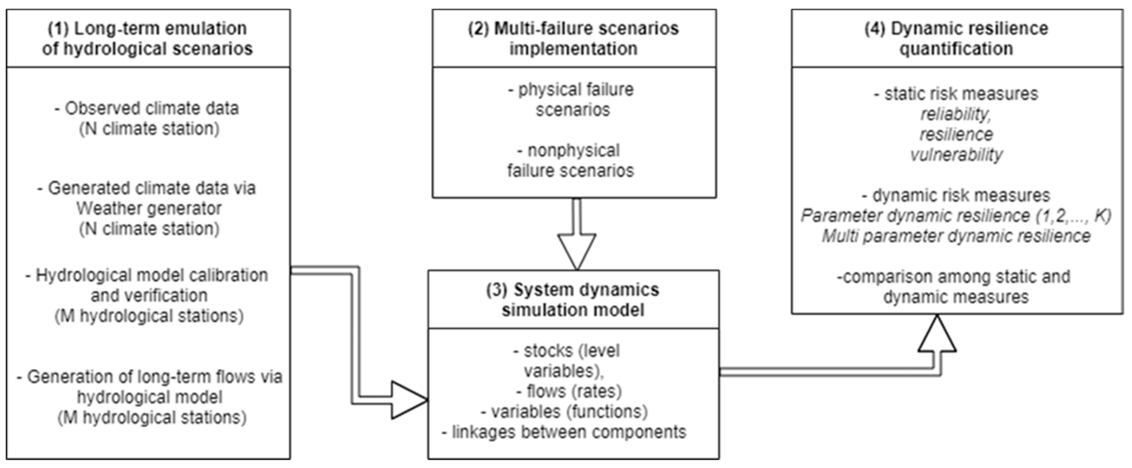
A general flow chart is shown in Figure 1 within the following four modeling steps: (1) long-term emulation of hydrological scenarios; (2) multi-failure scenarios implementation; (3) system dynamics modeling; (4) dynamic resilience quantification. A more detailed explanation regarding the framework for quantifying multi-parameter dynamic resilience for complex reservoir systems is provided in the next paragraphs.

2.1. Long-Term Emulation of Hydrological Scenarios

Climate data generation

Observed climate series (precipitation and air temperature) are usually not long enough to represent the range of events that can occur at the analyzed sites [3]. Therefore, weather generators can be used to overcome this issue generating long sequences of replicates using observed climate data (e.g., daily precipitation, maximum and minimum temperature).

There are three types of weather generator: parametric, semi-parametric and non-parametric. Parametric models have some disadvantages: they need to be statistically checked, they underestimate wet and dry spell lengths and do not preserve multisite correlations across all variables [20]. Semi-parametric models better reproduce the precipitation statistics, but they cannot be used for multi-site climate parameters generation [20]. Limitations of parametric and semi-parametric weather generators are overcome by non-parametric weather generators. Therefore, the non-parametric K-nearest neighbour weather generator (K-NN) is selected to reshuffle the historical data, with replacement. Each of the resampled values will then be perturbed to ensure unique values are generated that do not occur in the historical record.

Hydrological modeling

Later, the generated climate data is introduced to a next modeling step to generate long-term flows. Hydrological modeling is generally used to calculate flood events based on the known precipitation-runoff correlation at the specific watershed and available precipitation data. There are three types of hydrological model empirical, conceptual and physical [21]. In addition, hydrological models can be lumped, semi-distributed and distributed models [21].

To reproduce extreme hydrological events, it is deemed that physical based models should be used [22]. An example, employed in this research, is the semi-distributed Precipitation-Runoff Modeling System (PRMS). Its main applications are in the domain of water and natural resources management: evaluation of hydrological response to changes in watershed conditions or climate change, interaction of groundwater and surface water, etc. The PRMS model allows the user to discretize the watershed into hydrological response units, making a distributed parameter model. Model input are data from meteorological stations (daily precipitation and minimum and maximum daily temperature) and watershed characteristics (area, river segment length, slope). Observed flow data from hydrological stations are needed for model calibration. A series of soil layers and stream segments is used for the watershed model [22]. Runoff is simulated based on the outputs from different layers (e.g., impervious zone, soil zone, subsurface and groundwater). Snowmelt is determined based on the water and energy balance approach. The daily watershed response is calculated as a sum of the water balances of all hydrological response units, weighted by unit area [23].

Hydrological model calibration

Such a complex hydrological model with a large number of parameters needs to be calibrated quickly and effectively. Calibration of a hydrological model can be performed using a LUCA software for multi-objective automatic calibration [23,24].

Objective functions used in model calibration are absolute difference in observed and simulated data and normalized root mean square error as in [23].

Sum of absolute differences (AD) is given as follows:

$${\sum }^{}\mathrm{AD}={\sum }_{m=1}^{12}\left|OBS-SIM\right|$$

(1)

where ${\sum }^{}\mathrm{AD}$ is the sum of absolute differences, m is the month, and OBS and SIM are monthly mean observed and simulated values, respectively.

Normalized root mean square error (NRMSE) is defined as:

$$\mathrm{NRMSE}=\sqrt{\frac{{\sum }_{n=1}^{ndays}{\left(OB{S}_n-SI{M}_n\right)}^2}{{\sum }_{n=1}^{ndays}{\left(OB{S}_n-M{N}_n\right)}^2}}$$

(2)

where n is particular day in a time series, n_days is the total number of days, and OBS, SIM and MN are the observed, simulated and mean flow values.

Long time series generated in the weather generator are then used as an input to the calibrated hydrological model and long-term flows at hydrological stations can be obtained.

2.2. Multi-Failure Scenarios

Alongside hydrological model development, multi-failure scenarios of the reservoir system are proposed. These scenarios are based on the fact that the disturbances can affect each system element used to assess reservoir system performance [5]. Various disturbance scenarios are commonly simulated to assess the performance of a large number of interacting components, both physical (e.g., dam, gates, turbines) and nonphysical (e.g., operator). Physical failures include collapse of the dam, and/or collapse of any of its structural, mechanical, or electric components that may be caused by a system disturbance. Moreover, failures occur due to ageing of infrastructure, lack of maintenance, improper design or construction errors. Nonphysical failures happen when the system components and reservoir are not able to serve the intended purpose. These failures can be caused by improper operation and unexpected extreme natural conditions (e.g., floods). Given this, multi-failure scenarios are founded under the assumption that the functionalities of the system elements during hazardous events are reduced until the moment when they fully recover functionalities after reparation.

2.3. System Dynamics Simulation Model and Component Failure Model

Once the calibrated hydrological model is run under the generated climate data and multi-failure scenarios proposed, the inputs needed for the system dynamics simulation model (SDSM) are defined. System dynamics is a simulation modeling approach used to better understand the nonlinear behavior of multi-purpose reservoir systems over time. It is an object-oriented approach, based on a feedback systems theory [25].

The main components of the system dynamics model are stocks (level variables), flows (rates) into or out of the stocks, variables (functions) and linkages between these components. In this manner, decomposed representation of the multi-purpose water reservoirs can be devised, where all of the main interconnections between the system elements and functionalities are modeled. For the development of the model, typically Vensim DSS 8.1.1 software is used [26].

To model the system behavior in case of natural or man-made hazardous events, and all possible combinations of these events, it is important to adequately represent a physical drop of the functionalities of the particular elements. In the case of multi-purpose water reservoirs, some common elements can be identified, e.g., spillway, tailgate, hydropower plant, etc. Hypothetically, if an earthquake of a certain magnitude occurs, it can be assumed that one of the spillway gates will be jammed for a finite period of time. Naturally, the question of how to model this jamming failure arises. For this purpose, a concept of the functionality indicator α is introduced here.

This indicator can be defined for each particular element of the system. It can take only discrete predefined values, which are representative of the analyzed case. For the hypothetical case of the spillway gate jamming, the functionality indicator is used to reduce the spillway capacity in the model, by reducing the spillway crest length. If there are two spillway gates of equal length, and one gets jammed in a closed position, the parameter ${\alpha }_{sw}$ will take a value of 0.5, indicating that only half of the spillway crest length can be used for excess water overflow. Similarly, all of the system elements can have an appropriate $\alpha$ which will have discrete values:

$$\alpha =\left\{\begin{array}{cc}1,& Element is fully functional\\ 0<\alpha <1,& Reduced functionality of an element\\ 0& Element is non-functional\end{array}\right\}$$

(3)

At the beginning of the simulations, all $\alpha$ will have values 1. Once a certain event occurs, a group of system elements will be affected, thus reducing their $\alpha$ to a lower value. After a finite period of time elapses, needed for the repair of a particular element, $\alpha$ will restore a previous value.

2.4. Dynamic Resilience Quantification

Risk assessment of the multi-purpose reservoir system is estimated using static and dynamic measures. Static measures commonly used in engineering practice are reliability, resilience, and vulnerability, while the dynamic measure is expressed in the form of multi-parameter dynamic resilience estimating the risk as time dependent variable. A review of these measures is given in the next paragraphs, as they are used for comparison purposes.

Static risk measures

Reliability

Reliability $\alpha$ is the probability that a system is in functional state (S) [12].

$$\alpha =p\left[X_t\in S\right]$$

(4)

The state of a reservoir system X_t at time t can be either 0 (failure state) or 1 (success state) [4]:

$$X_t=\{\begin{array}{c}1, R_t\ge D_t\\ 0, R_t<D_t\end{array}$$

(5)

where R_t is release (or volume etc.) in time t and D_t is demand in time t. The reliability of a system is in that case:

$$\alpha =\frac{{{\displaystyle \sum }}_{t=1}^T{X}_t}{T}$$

(6)

where T is the total simulation time period [4].

Resilience

Resilience is a measure of system performance that describe how quickly a system will recover or bounce back from failure once a failure has occurred [12]. It is a conditional probability of a success state following a failure state [4].

$$\gamma =\left\{X_{t+1}\in SS|X_t\in F\right\}$$

(7)

It is also an inverse of the mean value of the time the system spends in the failure state [13]. Another interpretation is:

$$\gamma =\frac{M}{M_d}$$

(8)

where M is the number of individual continuous sequences of failure events and M_d is the total duration of all the failure events [4].

Vulnerability

Vulnerability is a measure of the likely magnitude of a failure event [12]:

$$\vartheta ={\sum }_{j\in F}{s}_j{e}_j$$

(9)

where s_j is the most severe outcome of the jth sojourn in unsatisfactory state and e_j is the probability of s_j being the most severe outcome of a sojourn into the unsatisfactory state. Vulnerability can be estimated as the mean value of the water deficit events v_j [13]:

$$\vartheta =\frac{1}{M}{\sum }_{j=1}^M{v}_j$$

(10)

where v_j is the water deficit volume during the failure event j and M is the total number of failure events.

Dynamic risk measures

Prior to the definition of the multi-parameter dynamic resilience, performance measures of a complex reservoir system need to be elaborated. Performance measures take values from 0 to 1. If there are no failures of the system elements, a performance measure is still equal to 0.

Performance measures are estimated for the reservoir and main river stream in the terms of two opposite system demands: hydropower generation and flood-protection. They take into account actual water storage for hydropower energy generation limited by its minimal ($V_{minWL}$) and maximal volumes ($V_{maxWL}$). Moreover, performance measures consider referent flow values ($Q$) within the main stream in the terms of regular ($Q_{regular flood defence}$) and emergency flood defence ($Q_{emergency flood defence}$), defined with respect to an existing rating curve.

Equations used for determination of a multi-purpose complex reservoir system performance measures are given as follows:

$$P_{Reservoir HPP}=\{\begin{array}{cc}0,& Reservoir volume\le V_{minWL}\\ 1,& Reservoir volume>V_{minWL}\end{array}$$

(11)

$$P_{Reservoir flood}=\{\begin{array}{cc}1,& Reservoir volume<V_{maxWL}\\ 0,& Reservoir volume\ge V_{maxWL}\end{array}$$

(12)

$$P_{River HPP}=\{\begin{array}{cc}1,& Q<Q_{regular flood defence}\\ 0,& Q\ge Q_{regular flood defence}\end{array}$$

(13)

$$P_{River HPP}=\{\begin{array}{cc}1,& Q<Q_{emergency flood defence}\\ 0,& Q\ge Q_{emergency flood defence}\end{array}$$

(14)

where $P$ stands for reservoir-hydropower performance ($P_{Reservoir HPP})$, reservoir-flood performance ($P_{Reservoir Flood})$, river-hydropower performance ($P_{River HPP})$, and river-flood performance ($P_{River Flood})$, while the referent flow in the main stream is defined as a flow for regular ($Q_{regular flood defence}$) and emergency flood defence ($Q_{regular flood defence}$).

Considering the values of the performance measures $P$ at any simulation step (Equations (11)–(14)), loss of system performance ($\rho )$ is defined in the general form as [4]:

$$\rho \left(t\right)=P_0\left(t-t_0\right)-{\sum }_{t_0}^{t}P$$

(15)

where $t$ is time simulation step and $t_0$ denotes the beginning of the system element failure.

Using the loss of system performance (Equation (15)), dynamic resilience is expressed as follows [4]:

$$r\left(t\right)=1-\left(\frac{\rho \left(t\right)}{P_0\left(t-t_0\right)}\right), r\left(t\right)\in \left[0,1\right]$$

(16)

Following Equation (16), multi-parameter dynamic resilience is defined:

$$\begin{gathered} r\left(t\right)={\left\{r_{reservoir flood}\times r_{reservoir flood}\times r_{river HPP }\times r_{river flood}\right\}}^{1/4} \\ ={\left\{\left(1-\frac{{\sum }_{t_0}^t{\rho }_{Reservoir HPP}}{P_0\left(t-t_0\right)}\right)\times \left(1-\frac{{\sum }_{t_0}^t{\rho }_{Reservoir flood}}{P_0\left(t-t_0\right)}\right)\times \left(1-\frac{{\sum }_{t_0}^t{\rho }_{river HPP}}{P_0\left(t-t_0\right)}\right)\times {\left(1-\frac{{\sum }_{t_0}^t{\rho }_{river flood}}{P_0\left(t-t_0\right)}\right)}_{ }\right\}}^{1/4} \end{gathered}$$

(17)

3. Pirot Reservoir System

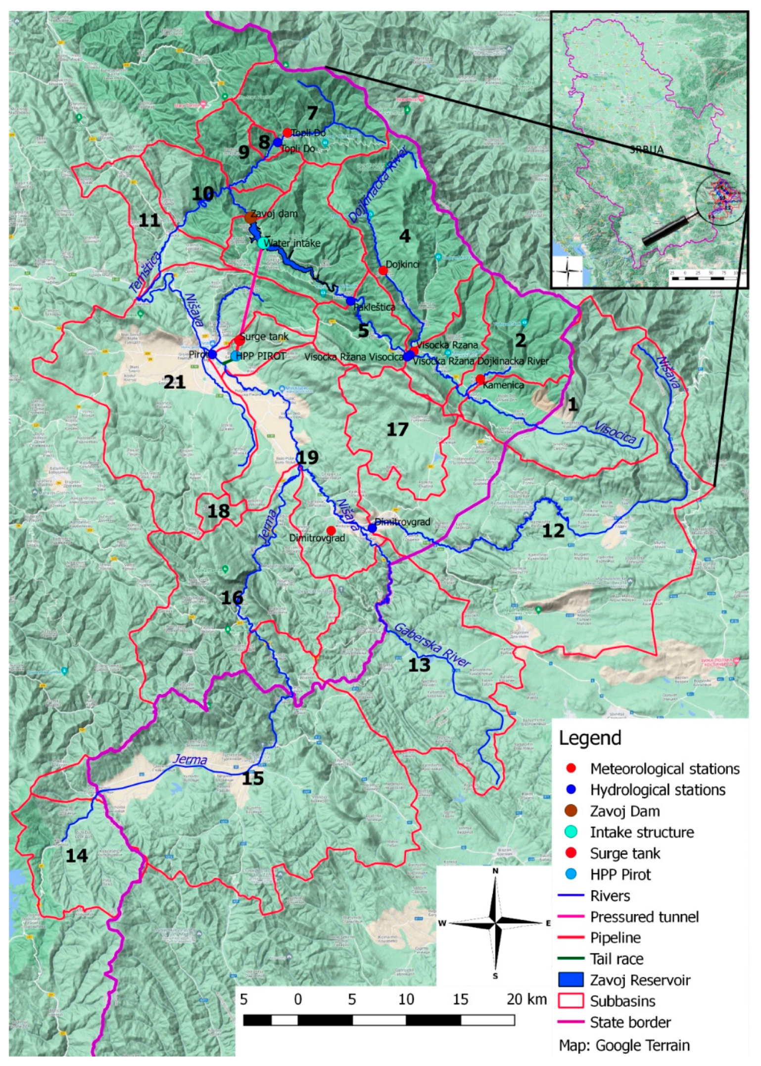
Pirot reservoir is located in the eastern Serbia, near the Stara Planina mountain and city of Pirot (Figure 2). It represents the multi-purpose reservoir system with main roles in hydro-energy generation and flood protection at the Nišava and Visočica rivers.

The Pirot reservoir located at the Visočica River has a whole basin area of 2940.85 km². It drains the water from the following river streams: the Nišava, Visočica (with a Zavoj Reservoir), Dojkinačka, Toplodolska, Temštica, Gaberska and Jerma Rivers. The hydrological regime at the Nišava River is influenced by the Visočica River since the pressured tunnel conveys to outflow from the Zavoj Reservoir through hydropower plant and compensation reservoir to the Nišava River upstream from hydrological station (h.s.) Pirot.

The observation network of the Pirot reservoir system consists of five meteorological stations (m.s.) and six hydrological stations located at the upstream Nišava river basin (Figure 3).

The Pirot reservoir system consists of (Figure 2): the dam on the Visočica river, Zavoj reservoir, pressured tunnel, surge tank, pipeline, hydroelectric power plant (HPP), tail race and compensation reservoir. The dam is earthen with upstream sloped clay core, double-layered upstream and downstream filters and rock embankment. A total volume of the dam is 1.5 × 10⁶ m³. The maximum dam height is 86 m. Dam length until spillway is 250.0 m, dam width at the crest is 10.0 m.

The maximum capacity of the bottom outflow is 62.5 m³/s. At the gates of the bottom outflow, there is a bypass pipeline used for discharging the environmental flow of 600 l/s.

The spillway has three segment gates, 9 m wide and 10.2 m high each. The maximum capacity of the spillway is 1820 m³/s. The pressured tunnel has 4.50 m in diameter with a length of 9093 m long. The hydropower plant has two vertical Francis turbines (installed power N_i =2 × 40 = 80 MW and installed water flow Q_i = 2 × 22.5 = 45.0 m³/s) and is designed to cover the peak electricity consumption, working around 4–5 h per day with an average annual production of around 120 × 10⁶ kWh.

Tail race is around 1300 m long, designed for a maximum flow of 45 m³/s. A major part of the flow is conducted to the compensation reservoir, and the minor part (8 m³/s) is discharged directly to the Nišava river. The compensation reservoir is located on the right riverside of the Nišava river and is designed to mitigate a water level oscillation in the Nišava river.

In terms of possible component failure, the following system components are analyzed: generators, segment gates on the spillway, leakage from the grout curtain, segment, and table gates on the compensation reservoir and Toplodolski tunnel.

4. Results

4.1. Long Term Evaluation of Hydrological Scenarios

The first step in the study includes the identification of the upper Nišava river basin, and the meteorological and hydrological stations within the river basin (Figure 3). Available data from meteorological stations (precipitation, minimum and maximum temperatures) and hydrological (flows) is collected. This data is essential for both the weather generator and hydrological model.

Climate data generation

Next, to perform long-term hydrological simulations, the KNN weather generator (KNNWG) [20,29] is used to generate time series of precipitation and temperature for the time period of 1000 years based on observed meteorological data. Observed meteorological daily data (precipitation and air temperature) from 5 stations (m.s. Dimitrovgrad, m.s. Topli Do, m.s. Visočka Ržana, m.s. Dojkinci and m.s. Kamenica Dimitrovgradska) given in Figure 3 are used as input to the weather generator. The available period for meteorological data (daily precipitation and minimum and maximum daily temperatures) on m.s. Dimitrovgrad is from 1950 to 2016 [30]. For all other stations (m.s. Topli Do, m.s. Dojkinci, m.s. Visočka Ržana and m.s. Kamenica Dimitrovgradska), data are available only for precipitation (1950–2016).

To illustrate the generated climate data, theoretical extreme precipitation values for return periods of 100 and 1000 years are presented in

Table 1. Theoretical values of observed and generated extreme precipitation for meteorological stations analyzed.

	m.s. Dojkinci, Observed Precipitation 1950–2016				m.s. Dojkinci, Generated Precipitation for 1000 Years λ = 0.8
Return Period:	Pearson III	LogPearson III	Gumbel	GEV	Pearson III	LogPearson III	Gumbel	GEV
1000 years	182.5	204.6	159.1	188.5	806.0	807.5	365.9	606.4
100 years	126.6	124.8	118.2	121.1	343.7	266.0	252.4	285.2
	m.s. Dimitrovgrad, observed precipitation 1950–2016				m.s. Dimitrovgrad, generated precipitation for 1000 years λ = 0.8
1000 years	163.9	197.8	150.5	171.2	764.0	670.7	345.3	579.4
100 years	116.5	119.4	111.7	113.2	324.1	233.4	237.3	267.9
	m.s. Kamenica, observed precipitation 1950–2016				m.s. Kamenica Dimitrovgradska, generated precipitation for 1000 years λ = 0.8
1000 years	149.2	177.2	145.6	156.6	837.9	723.8	376.2	637.2
100 years	109.6	113.8	108.7	108.3	352.8	236.9	257.1	290.6
	m.s. Topli Do, observed precipitation 1950–2016				m.s. Topli Do, generated precipitation for 1000 years λ = 0.8
1000 years	155.8	180.2	150.6	163.5	763.1	733.8	347.5	574.4
100 years	113.9	116.8	112.4	112.3	326.5	253.5	240.3	271.3
	m.s. Visočka Ržana, observed precipitation 1950–2016				m.s. Visočka Ržana, generated precipitation for 1000 years λ = 0.8
1000 years	145.8	180.7	141.9	152.9	720.6	578.7	327.4	551.9
100 years	107.7	113.9	106.7	106.4	307.5	216.1	226.0	254.2

. The results cover several theoretical distributions including the Pearson III, Log Pearson III, Gumbel and General Extreme Values (GEV) distributions. For instance, it is shown that extreme generated precipitation under the assumption to follow the Pearson III distribution for return periods of 100 and 1000 years are respectively 2.9 and 4.9 times greater than the observed values. Similarly, the rest of the theoretical distributions (LogPearson III, Gumbel, GEV) indicate the same increase of extreme precipitation ranging from 2.0 to 3.7.

Hydrological modeling

Later, the generated climate data is introduced to a hydrological model to generate long-term flows. Here, the Precipitation-Runoff Modeling System PRMS [22,31] is applied. Hydrological model calibration is performed by using the automatic multiple-objective stepwise calibration within the USGS LUCA (Let Us CAlibrate) software [24]. Hydrological data used for the model calibration are gathered from the Republic hydrometeorological service of Serbia and Public enterprise Elektroprivreda Srbije [32]. Iterations consisted of four steps and up to six rounds are conducted until the objective function criteria is satisfied. There are specific groups of model parameters, calibrated using the literature [23].

Hydrological model calibration

Results of hydrological model calibration and verification for selected hydrological stations (h.s. Visočka Ržana—Dojkinačka river, h.s. Pakleštica—Visočica river, h.s. Pirot—Nišava river) are depicted in Figure 4. Modeled daily flows show better agreement in the calibration phases with the observed values, while the agreement in the verification phase is somewhat lower. It is worst noting that hydrological modeling is performed using available daily precipitation sums over the Nišava river basin in Serbia, while the most upstream parts of the river basin (subbasins 14, 15, 16, 33) are not covered by the precipitation monitoring network (Figure 3). A lack of measured data results in a somehow lower agreement between observed and simulated daily flows at the sites of hydrological stations used. In the next step, the hydrological model is run using generated precipitation and minimum and maximum temperatures for a period of 1000 years with the aim of calculating the long-term flow sequences with the same length as the input data.

Similarly, as for the case of the climate data, the generated flows are illustrated for hydrological stations in the terms of theoretical values of extreme observed and simulated flows. The results in

Table 2. Theoretical values of observed and generated extreme flows for hydrological stations analyzed.

	h.s. Dimitrovgrad, Observed Flow 1990–2016				h.s. Dimitrovgrad Modeled Flow 1000 Years
Return Period:	Pearson III	LogPearson III	Gumbel	GEV	Pearson III	LogPearson III	Gumbel	GEV
1000 years	122.5	121.9	120.7	129.0	963.8	736.4	413.8	740.8
100 years	83.5	80.9	85.1	81.3	386.0	206.5	271.9	308.9
	h.s. Visočka Ržana, Dojkinačka River observed flow 1990–2015				h.s. Visočka Ržana, Dojkinačka River modeled flow 1000 years
1000 years	125.6	179.7	133.0	132.4	755.2	428.5	332.5	576.1
100 years	90.5	103.3	96.0	89.8	311.1	171.7	223.4	253.4
	h.s. Visočka Ržana, Visočica observed flow 1961–1974				h.s. Visočka Ržana, Visočica modeled flow 1000 years
1000 years	225.1	271.5	280.2	232.9	1350.4	874.7	590.2	1032.0
100 years	173.4	188.7	205.3	174.9	551.7	293.4	394.1	447.4
	h.s. Pakleštica, observed flow 1990–2016				h.s. Paklestica, modeled flow 1000 years
1000 years	314.6	215.0	398.8	318.6	1590.6	1046.4	693.3	1218.1
100 years	243.9	200.4	287.5	246.6	647.9	336.9	461.9	524.1
	h.s. Topli Do, observed flow 1990–2016				h.s. Topli Do, modeled flow 1000 years
1000 years	94.6	117.4	116.1	97.7	349.1	154.2	158.7	269.1
100 years	72.0	80.9	83.8	72.7	149.1	83.8	109.6	123.0
	h.s. Pirot, observed flow 1950–1989				h.s. Pirot, modeled flow 1000 years
1000 years	254.2	281.2	310.9	256.1	4164.0	2067.7	1770.3	3191.7
100 years	203.0	216.2	231.1	204.9	1649.1	454.6	1152.9	1314.3

suggest that the simulated values exceed observed ones. For example, for the GEV distribution these values exceed the observed levels several times; the simulated values are greater by 1.8 and 4.2 times for the 100 and 1000 return periods, respectively.

4.2. Multi-Failure Scenario Implementation

To assess the risk of a multi-purpose reservoir system, multi-failure scenarios (SC) as the input for the system dynamics simulation model are generated. Multi-failure scenarios assume that the disturbances can affect each system element. The scenarios represent physical failures of the structural, mechanical, and electric system components of the Pirot reservoir system. Firstly, possible single failures of the following system elements are assumed: generators, segment gates on the spillway, leakage from the grout curtain, segment, and table gates on the compensation reservoir and Toplodolski tunnel (

Table 3. Description of a single failure scenario event.

Number of Failure Event	Element:	Disturbance Scenario	Active/Passive Element	Number of Elements	Functionality Indicator Values	Failure Start and End Time (h)	Failure Duration (h)
1	HPP generators	Generator failure	active	2	αHPP = {0, 0.5, 1}	7129–15,889	8761 (1 year)
2	Spillway segment gates	Gate failure	active	3	αSWl = {0, 0.33, 0.67, 1}	7129–11,509	4381 (6 months)
3	Dam leakage	Earthquake/ leakage	passive	1	αEARTHQUAKE  $\in${0, 15}	7129–24,649	17,521 (2 years)
4	Toplodolski Tunnel	Water intake gate failure	passive	1	αTUN_TD = {0, 0.5, 1}	7129–10,009	2881 (4 months)
5	Compensation reservoir segment gates to Nišava River	Gate failure	active	2	αCRSG = {0, 0.5, 1}	7129–9289	2161 (3 months)

). During these failures, the performance measures of the system elements are reduced, and therefore functionality indicators for each system element are employed in the range from 0 to 1. Moreover, failure start-time and end-time are proposed alongside the duration of a single failure. By using the possible single failure events, multi-failure scenarios (from 1 to 5) are defined, combining them in the manner shown in

Table 4. Description of failure scenarios (SC) consisting of multi-failure events.

No.	Scenario Description	Failure Event Included
		1 Generator Failure (HPP Working with 50% Capacity)	Spillway Segment Gates Failure (33% Working)	Reservoir Leakage is 15× Higher than Usual Due to Earthquake	Toplodolski Tunnel Failure (Working with 50% Capacity)	1 Compensation Reservoir Segment Gate Failure (Working with 50% Capacity)
SC0	Reference scenario
SC1	1/2 HPP generators	x
SC2	1/2 HPP generators 1/3 spillway segment gates	x	x
SC3	1/2 HPP generators 1/3 spillway segment gates 15x dam leakage	x	x	x
SC4	1/2 HPP generators 1/3 spillway segment gates 15x dam leakage 1/2 Toplodolski Tunnel	x	x	x	x
SC5	1/2 HPP generators 1/3 spillway segment gates 15x dam leakage 1/2 Toplodolski Tunnel 1/2 Compensation reservoir segment gates	x	x	x	x	x

.

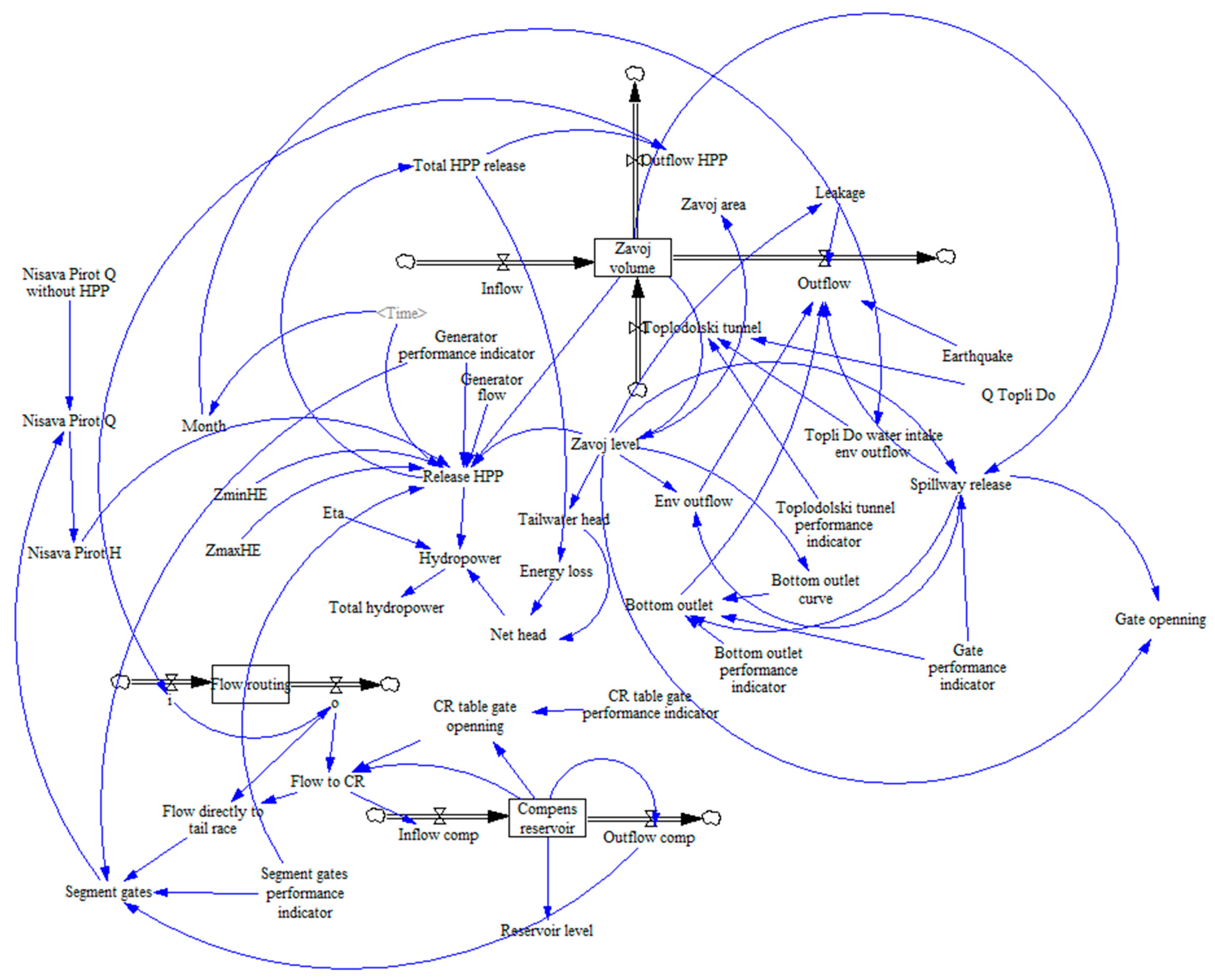
4.3. System Dynamics Simulation Model

A system dynamics simulation model (SDSM) of the Pirot reservoir system (Figure 5) is developed in Vensim software (version DSS 8.1.1) [26] with the final aim of calculating system performance and resilience over time. The main components of the developed system dynamics model are stocks (level variables), flows (rates), variables (functions) and linkages between these components (Figure 5).

The Zavoj Reservoir volume is represented as a level variable. There are two inflows into the reservoir: main inflow through the Visočica River and inflow from the Toplodolski tunnel. The first outflow is flow for electricity generation passing from the Zavoj reservoir through the pressured tunnel and pipeline to the Pirot hydropower plant. The second outflow is downstream of the Zavoj dam consisting of environmental outflow (600 l/s), spillway release, bottom outlet and leakage from the Zavoj reservoir. Spillway release is regulated with three segment gates and the proposed model is programmed to calculate their openings. Hydropower generation is a function of the hydropower release, net head and turbine efficiency coefficient. Leaving the hydropower plants, hydropower outflow is routed to the compensation reservoir. There are two types of gate that regulate the outflow from the hydropower plant. Namely, two segment gates regulate the outflow from the compensation reservoir to the river stream (Nišava river), while five table gates regulate inflow into the compensation reservoir. If the water level at the Nišava river (h.s. Pirot) surpasses the regular flood defence level (RFD = 365.57 m a.s.l.), the hydropower plant suspends turbine outflows until the water level decreases to under the aforementioned water level.

The input data for the SDSM are the proposed failure scenarios from SC1 to SC5 and generated flows at the domain of the model (the Zavoj Reservoir at the Visočica River and h.s. Pirot at Nišava river). It is assumed that multi-failure scenarios occur during unexpected extreme natural conditions (e.g., floods, earthquakes) which rapidly decreases the functionality of the system element. Therefore, the functionality indicators of the system element are used as the inputs for the system dynamics simulations (Table 3).

For the generated flows, the 10-year periods with the most severe flood event are sampled assuming that the failure of the system elements falls at the same time as the time of peak flow. It should be noted that the first simulation scenario (SC0) without any failure of the system elements is carried out, in order to be compared with the results under the disturbed reservoir system (SC1–SC5).

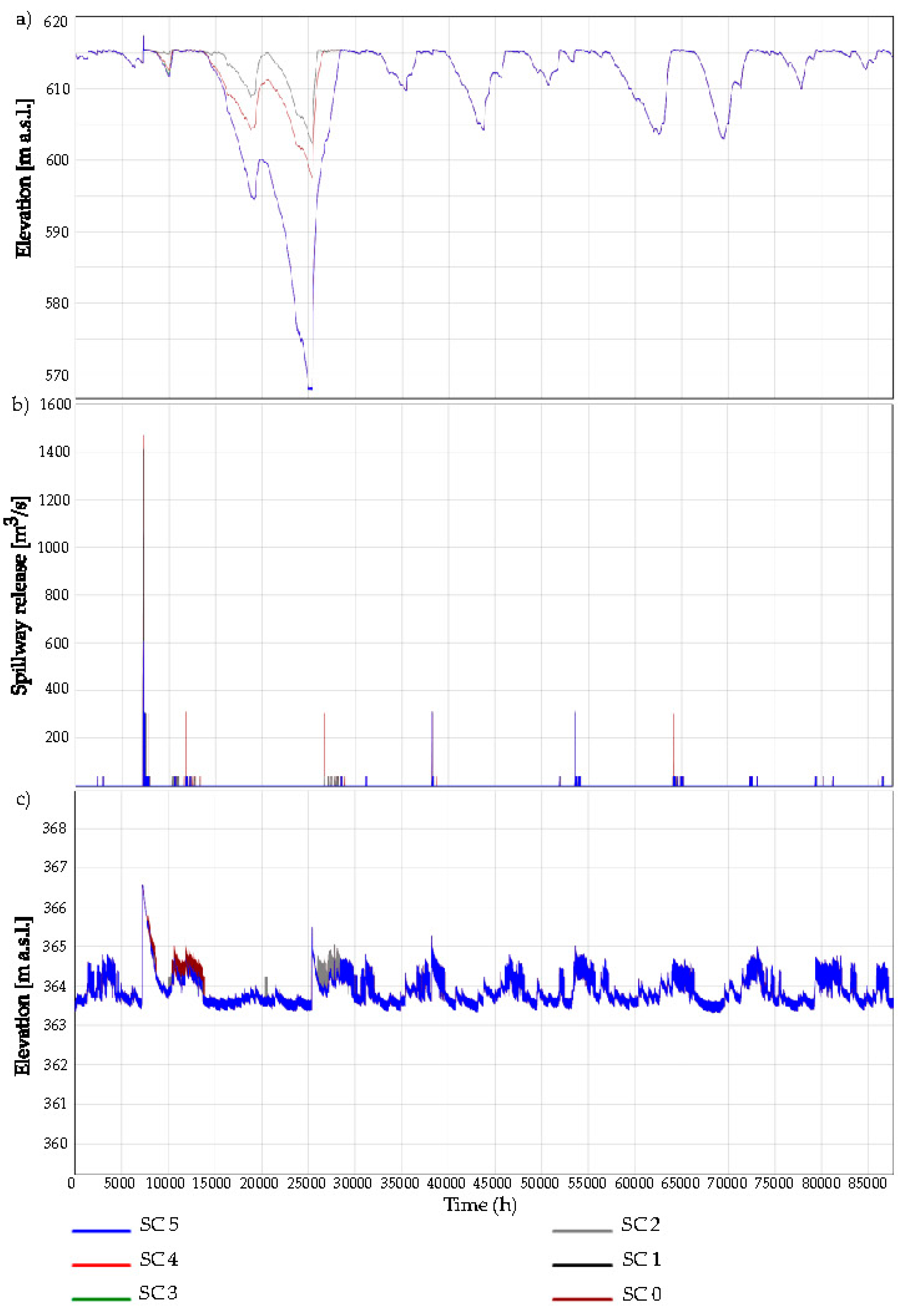
The results of the system dynamics simulation model for five failure scenarios are shown in Figure 6. For five scenarios considered, the Zavoj reservoir levels, spillway release and Nišava level at h.s. Pirot are shown in Figure 6a–c, respectively.

For the case of SC1 (black line on the graph), the results show that water levels in the Zavoj reservoir are higher compared to the referent scenario (SC0—dark red line). During the flood event (starts at the 7202nd time step), the water level in the reservoir overcomes the NWL (615 m a.s.l) leading to the spillway overflow. Then, water levels continue rising to the MaxWL at the 7227th time step. During the simulation period, there is enough water in the HPP release. However, when the water levels at the Nišava River (h.s. Pirot) overcome the RFD, the HPP needs to restrict the turbine outflows to reduce the water levels alongside the protected area (city of Pirot).

At the 7129th time step, earthquake consequences result in the failures of two spillway segment gates, leaving only one gate in function (SC2). The spillway cannot fulfil its duty starting from the 7218th time step, so the water level rises to 617.49 m a.s.l. (the dam crest elevation is 617.5 m a.s.l.). Although these two segment gates remain out of function until the 11,509th time step, the water level reaches the same values as in the case of SC1 and SC0 starting from the 7246th time step.

If the earthquake degrades the soil layer around the Zavoj Dam, it results in increased leakage from the reservoir (SC3). Therefore, the water level drops up to the MinWL (the reservoir would be empty in 24,929th time step), remaining at the same level until the 25,360th time step.

If the Toplodolski tunnel fails (SC4), the inflow into the Zavoj Reservoir rapidly decreases (water levels drop by 30 cm in the period between 8600th and 10,450th time step). On the other side, the leakage from the SC3 is greater than the inflow reduction caused by failure of the Toplodolski tunnel, making the differences between SC3 and SC4 negligible.

The next failure scenario (SC5) includes all the previous failures with additional pressure brought about by the failure of one compensation reservoir segment gate. Because the compensation reservoir segment gates failure is only 3 months, while the generator failure is one year starting from the same time, the hydropower outflow is already reduced by 50% due to generator failure. Therefore, hydropower flow reduction due to gate failure does not affect the system functionality.

4.4. Dynamic Resilience Quantification

Prior to the quantitative dynamic resilience assessment, the static risk measures have to be estimated to be compared with the dynamic risk measures. The minimal and maximal hydropower plant working levels are used to assess the performance measures, and hydropower resilience. In the case of flood resilience, the regular flood defence level in the Nišava River and simulated water levels are considered as system performance measures leading to flood dynamic resilience assessment. Considering hydropower and flood dynamic resilience, the multi-parameter dynamic resilience of the Pirot reservoir system is finally assessed.

Static measures

The static measures for risk assessment are calculated using Equations (6), (8) and (10). Although reliability, resilience and vulnerability are calculated within each simulation time step, only the final estimates at the end of simulation are relevant for risk assessment of the Pirot reservoir system.

Prior to estimation of the reservoir system reliability, the states of the reservoir system X_t are calculated for each time step using Equation (5). Using the defined states of the Pirot Reservoir System (X_t), the reliability of the system is defined by Equation (6).

To define how quickly the Pirot reservoir system is recovered after a hazardous event, system resilience is calculated accounting for the number of failure event and their total duration by applying Equation (8). Moreover, the system vulnerability is calculated with Equation (10). Precisely, the total number of failure events is equal to the number of times the system is not functional (X_t = 0), while the total water deficit is calculated by summing the deficits during the failure events considered.

The resulted static risk measures for the Pirot reservoir system are given in

Table 5. Static risk measures (reliability, resilience, vulnerability) of the Pirot reservoir system.

State of the System:	Static Measures:	SC0	SC1	SC2	SC3	SC4	SC5
Reservoir HPP	Reliability (-)	1.0	1.0	1.0	0.998	0.998	0.998
	Resilience (1/s)	1.0	1.0	1.0	0.163	0.167	0.167
	Vulnerability (m3)	0	0	0	3.31 × 105	3.25 × 105	3.25 × 105
Reservoir flood	Reliability (-)	1.0	1.0	1.0	1.0	1.0	1.0
	Resilience (1/s)	1	1	0.043	0.042	0.043	0.043
	Vulnerability (m3)	2.25 × 105	9.43 × 104	1.40 × 108	1.44 × 108	1.34 × 108	1.34 × 108
River HPP	Reliability (-)	0.993	0.994	0.994	0.994	0.994	0.994
	Resilience (1/s)	0.101	0.044	0.044	0.044	0.044	0.044
	Vulnerability (m3)	5.55 × 103	1.29 × 104	1.29 × 104	1.29 × 104	1.29 × 104	1.29 × 104
River flood	Reliability (-)	0.998	0.998	0.998	0.998	0.998	0.998
	Resilience (1/s)	0.006	0.006	0.006	0.006	0.006	0.006
	Vulnerability (m3)	2.87 × 105	2.87 × 105	2.87 × 105	2.87 × 105	2.87 × 105	2.87 × 105

for the state of the system considered (Reservoir HPP, Reservoir flood, River HPP, River flood).

The results from Table 5 show that the reliability of the system within the failure scenarios (from SC1 to SC5) are generally greater than 99.3%. The reservoir HPP resilience has a maximal value for SC0, SC1 and SC2, but it drops to 0.163 in SC3 when the leakage drains the Zavoj reservoir. Moreover, it keeps a similar level for SC3 and SC4 (0.167). The vulnerability of the reservoir HPP is most highlighted when the leakage drains the reservoir (SC3). However, the reservoir flood vulnerability is pointed out when the spillway segment gates fail (SC2).

Dynamic measures

Following Equations (11)–(17), a separate system dynamic module is developed to quantify the multi-parameter resilience of the Pirot reservoir system. The module integrates the functional indicator of the system elements taking the discrete values of system functionality from 0 to 1 (Equations (11) and (12)). The values of the functional indicator related to the system element depend on the multi-failure scenario selected (Table 3).

Accounting for the functional system indicators within the multi-failure scenarios, the system performance measures are estimated by applying Equations (11)–(14). Using the estimated system performance measures, the dynamic resilience is estimated in the terms of hydropower generation, $r_{Reservoir HPP}=f\left(P_{Reservoir HPP}\right)$ and $r_{River HPP}=f\left(P_{River HPP}\right)$, and flood-protection, $r_{Reservoir Flood}=f\left(P_{Reservoir Flood}\right)$ and $r_{River Flood}=f\left(P_{River Flood}\right)$.

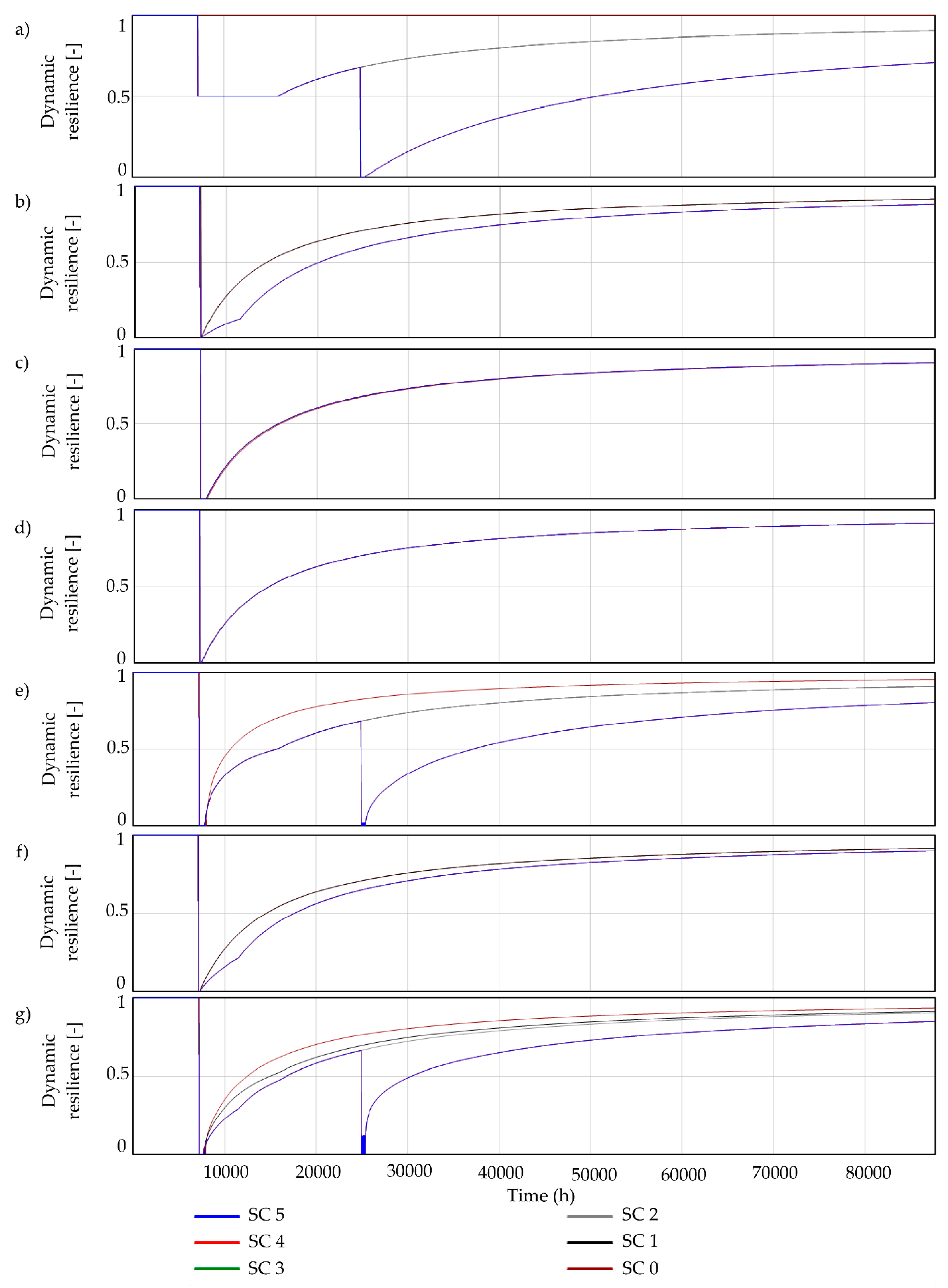
Applying Equation (17), the multi-parameter resilience of the Pirot reservoir system is then determined. The reservoir HPP and reservoir flood dynamic resilience are shown in Figure 7a,b, respectively. Moreover, the river HPP and river flood dynamic resilience are depicted in Figure 7c,d, respectively. Figure 7e represents the hydropower dynamic resilience ($r_{HPP}$), while Figure 7f depicts the flood dynamic resilience ($r_{Flood}$). Finally, the multi-parameter dynamic resilience for the Pirot reservoir system is shown in Figure 7g.

It can be seen from Figure 7g, the multi-parameter dynamic resilience of the Pirot reservoir system for SC0 drops to zero value at the 7203rd time step (when the water levels at the Nišava reach reaches the RFD level) remaining the zero value until the 7732nd time step. Then, it starts to oscillate slightly above zero until reaching 0.935 at the final time step. Once the one hydropower generator fails (SC1), multi-parameter dynamic resilience drops from 1 to 0.841 at the 7130th time step, keeping constant value until the 7202nd time steps when high flows at the Nišava river disable hydropower generation. The difference between SC1 and SC2 is that the two segment gates failure in SC2 cause the additional reduction of system functionality and decrease of multi-parameter dynamic resilience. Therefore, for SC2 dynamic resilience is somewhat reduced compared to SC1 and it reaches the value of 0.905 at the final time step.

In the case of SC3, the multi-parameter dynamic resilience remains at the same level as SC2 until leakage reduces the level in reservoir at the 24,929th time step. Then, the multi-parameter resilience drops at the zero value. The Pirot reservoir system is recovered at the 25,361st time step when the leakage from reservoir is reduced filling the reservoir at the nest simulation steps. Within this scenario, dynamic resilience reaches the lowest level (0.851) at the final simulation step.

The last two scenarios (SC4 and SC5) have the same values of multi-parameter dynamic resilience as in the case of SC3. Therefore, the Toplodolski Tunnel failure (SC4) and compensation reservoir segment gate failure (SC5) do not affect dynamic resilience since the additional pressures at the system do not significantly reduce the functionality of the system as a whole. The reason lies in the fact that the reservoir is still empty and cannot be filled in during the rest of the simulation period.

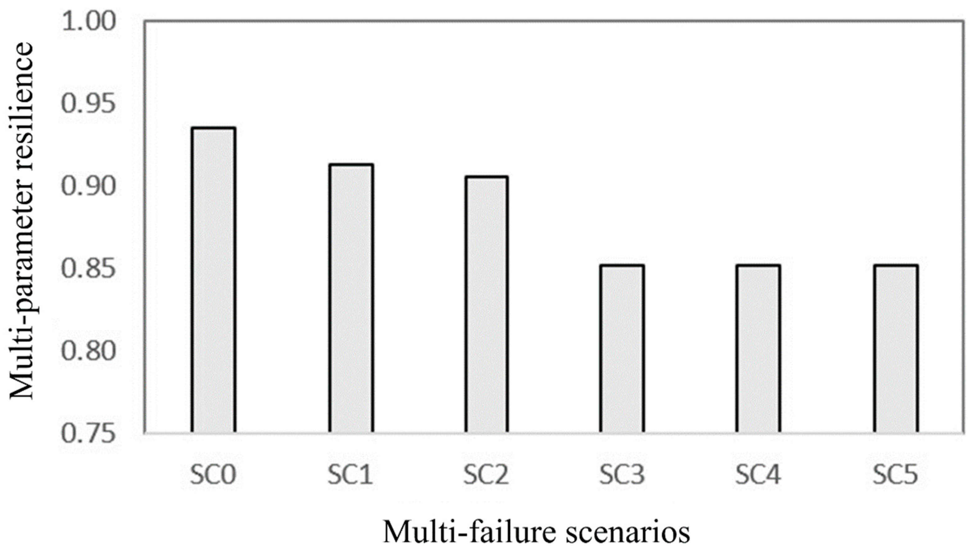
The values of multi-parameter dynamic resilience are summarized from the start to the end of the simulations (Figure 8) and normalized in the way that final values are ranged between 0 to 1. The result suggests a general increase in the risk assessment following the severity of the failure scenarios. The most resilient scenario (SC0) considers only the extreme flood event without any additional failure of the system element. However, it decreases the functionality of the system significantly (0.935). The multi-parameter resilience is in the range from 0.913 to 0.851 under the failure of the hydropower plant, spillway gates and leaking from the reservoir (SC1, SC2, SC3). Moreover, additional stresses on the reservoir system (SC4 and SC5) do not increase the risk since dynamic resilience keeps the value at the same level as for SC3.

5. Discussion

From Figure 6 and Figure 7, depicting water level variations and spillway flow rate as well as the changes in dynamic resilience, in the analyzed time period, it can be seen that the system dynamic model managed to adequately represent the effects of the single and multi-component failures. One of the key advantages of the novel explicit approach for the component failure modeling, compared to the stochastic approach [3], is the possibility of modeling the effects of the system investments. For example, if the system dynamics analysis based on the multi-parameter resilience assessment identifies a particular element (e.g., segment gates) as a weak point of the reservoir system, future investment projects should consider the possibility of the revitalization of these gates or of acquiring spare parts, which would reflect in the reduced failure duration. Now the same set of scenarios, with reduced failure duration for segment gates, can be run through the system dynamics model, to verify the effects of this particular investment decision.

The quantification and modeling of the dynamic resilience of a complex system are still under debate since the modeling steps are generally proposed for a particular system needed to mimic its nonlinear system behavior [33]. In general, the comparison of the results which quantify the dynamic resilience is difficult due to the following reasons [34]: various linked elements of a resilience assessment, and the selected simulation time step and total simulation period. However, the normalized form of a multi-parameter dynamic resilience can be compared with the static risk measures (e.g., reliability) obtained for the Pirot reservoir system, as the same models and failure scenarios are used for risk assessment.

Prior to the multi-parameter dynamic resilience assessment, the static risk measures are determined since they are commonly used to estimate water reservoir related risks. Considering the static measures provided in Table 5, similar results are obtained in the literature [4], where the values of reliability are generally high (>0.945) compared to static resilience (0.0097–0.0275). Taking into account the changing climate conditions, system resilience can also be lower than reliability in the assessment of the reservoir performance [35]. The relationship between static risk measures (Table 5) indicates the inverse proportionality between resilience and vulnerability. Resilience shows high values, while the system vulnerability seems to be low, leading to the fact that the reliable reservoir systems are more resilient and less vulnerable [13]. Therefore, the failure scenario which preserves the high level of system performance is the one with high reliability or resilience values. In the terms of hydropower generation resilience, these scenarios are SC0, SC1 and SC2, while flood-protection resilience targets scenarios SC0 and SC1. Other considered scenarios express a low level of static resilience, although the system reliability is still high.

By comparison with multi-parameter dynamic resilience, the static risk measures underestimate the risk stemming from the hazardous events, while dynamic resilience provides a successful tool that quantifies the risk over simulation time. For instance, the reliability of the system is in the range from 0.993 to 1, while the multi-parameter resilience ranges from 0.851 to 0.935 (Figure 8). The severe failure scenarios, for example, SC1 and SC3, slightly decrease the system reliability which is not in the line with the reduced system functionality which is indicated by dynamic resilience. However, the multi-parameter dynamic resilience does not reach the pre-disturbance level overall simulation time steps even if the system reaches full performance level. This can be attributed to the fact that the disturbed reservoir system requires additional time to recover system functionality [4].

Moreover, the multi-parameter dynamic resilience can assist to target the weak points of the Pirot reservoir system. The results in Figure 8 suggest that the overall functionality of the Pirot reservoir system is highly vulnerable to the increased leakage from the reservoir and failure of the spillway (SC2, SC3). Additionally, the failure of the spillway gate stresses the system functionality significantly (SC1). However, the system is still robust when the spillway gate at the compensation reservoir and the Toplodolski tunnel fail (Figure 8).

6. Conclusions

This study proposes a new concept of multi-parameter dynamic resilience for a complex reservoir system providing the link between the reservoir system and its environment using an inner control loop. The proposed concept is founded upon system dynamics simulation techniques and functional indicators of the system element enabling it to be widely applied to multi-purpose reservoir systems.

The proposed concept is applied at the Pirot reservoir system located in Serbia. This complex reservoir system is selected since it needs to satisfy several opposite demands, the most important being flood-protection and hydro-energy generation. It lies at a flood-prone region in southeast Serbia where snow-related processes have an impact on flood genesis. Moreover, it assists in covering “peak hours” when demand for electricity in Serbia are highest. Considering these issues, the proposed concept enables the assessment of multi-parameter dynamic resilience enveloping the aforementioned opposite demands and suggesting the adequate operation of reservoir systems under multi-failures. Moreover, this concept is generic and offers application on alternative reservoir systems by changing the reservoir inflows, structure of the system elements and operational rules. It is worth mentioning that the application of the proposed concept to alternative study requires a redefinition of dynamic resilience measures following the system functions (e.g., water supply, drought management, environmental services and recreational activities).

This concept is developed under the systems dynamic approach integrating the chain of the models. Firstly, the non-parametric weather generator is applied to simulate climate variables at the upper Nišava river basin for the 1000-year time period. Then, the hydrological model of the Nišava River and main tributaries is developed to convey climate parameters to flows at the sites of interest. Finally, the SDSM of the Pirot reservoir system is developed to mimic its regular operations. The integrated chain of models is then used to assess the multi-parameter dynamic resilience under the most severe flood event alongside failure scenarios related to the reduced functionality of system elements.

Multi-parameter dynamic resilience integrates the risk related to the water and environmental systems. First, the multi-purpose Pirot reservoir system with its elements is used in the terms of flood-protection of downstream area (city of Pirot) and hydropower energy generation. It is driven by operational rules depending on the water levels in reservoirs and inflows. Next, the environmental system is presented by a hydrological model where the climate drivers force the model outputs. High flows at downstream river sections (Nišava river) disable hydro-energy generation with the aim of keeping the water levels at acceptable elevation. Therefore, the predefined inner control loop is introduced to link the water and environmental systems by controlling the turbine outflows. Moreover, a concept of functional indicators is proposed to offer a bound between multi-failure scenarios of the system element and reservoir system itself. Functional indicators, therefore, implicitly deduced a system element functionality, weighting it with the standardized numerical values.

Using predefined inner control loop and functional system indicators the multi-parameter dynamic resilience estimates the risk of the Pirot reservoir system over time considering its main purposes: flood-protection and hydro-energy generation. Moreover, the multi failure scenarios are introduced with the aim of targeting vulnerable system elements. For instance, the most sensitive system elements are shown to be leakage from the reservoir, spillway gates and hydropower plant, rather than a failure of the compensation reservoir spillway and Toplodolski tunnel. Therefore, the proposed approach should be used as a stress-test for the reservoir system’s capability of indicating weak points in the usage.

The proposed dynamic resilience is also compared with the traditional static measure. Static measures (reliability, resilience, vulnerability) do not provide variability in the risk assessment during the failure scenarios causing insufficient insight into the ability of the system to respond and recover from the failure scenarios. For instance, the system reliability does not recognize the risks related to the multi-failure scenarios or underestimate them. Another point is that multi-parametric dynamic resilience is not time-independent and defines the risk at each simulation step. Therefore, multi-parameter resilience can be used for proposing or updating reservoir operation strategy or forecasting system performance after hazardous events like major floods or earthquakes.

Future research can be oriented in two directions. First, to reduce the uncertainty related to functionalities of the critical system elements within the proposed concept, the results from the numerical dam safety model needs to be incorporated within the concept for dynamic resilience quantification [36] Such a numerical model is capable of providing more realistic behaviour of the dam under earthquakes; for instance, leaking from the reservoir and failure of the spillway gates may be determined on a physical basis rather than using a heuristic approach presented in this study. Second, the extraction of interpretable knowledge from a large amount of data gathered through the system dynamic model simulations under a number of generated failure scenarios can provide a solid basis for improvements in the dynamic resilience assessment. This can reduce uncertainties due to the limited number of failure scenarios considered.