
The Influence of Fracture on the Permeability of Carbonate Reservoir Formation Using Lattice Boltzmann Method


 and
and 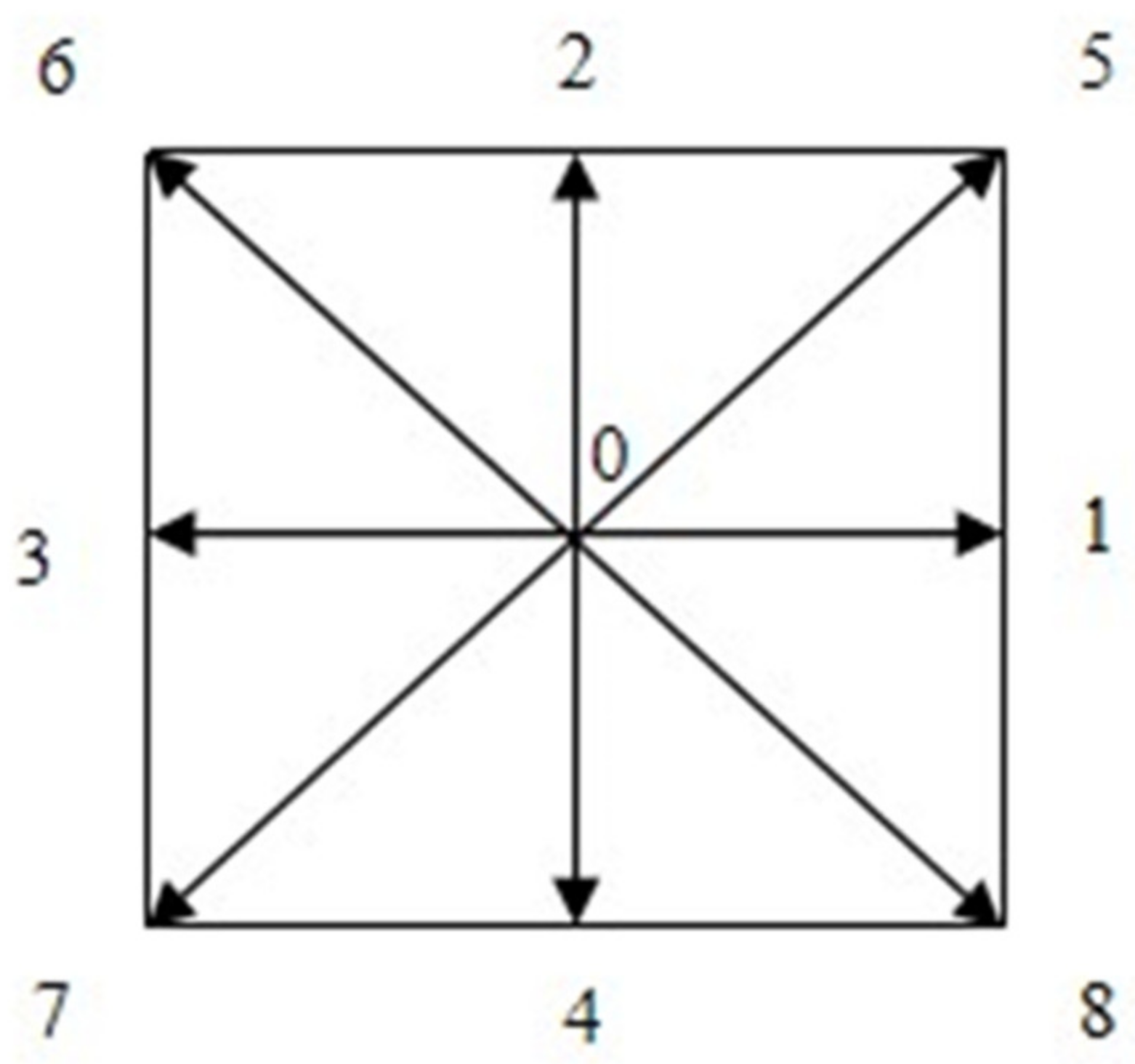
Abstract
:1. Introduction
2. Numerical Method and Physical Model
2.1. LBM
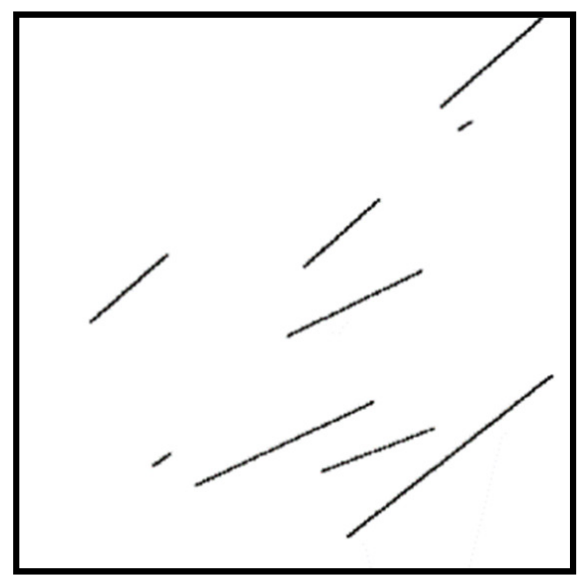
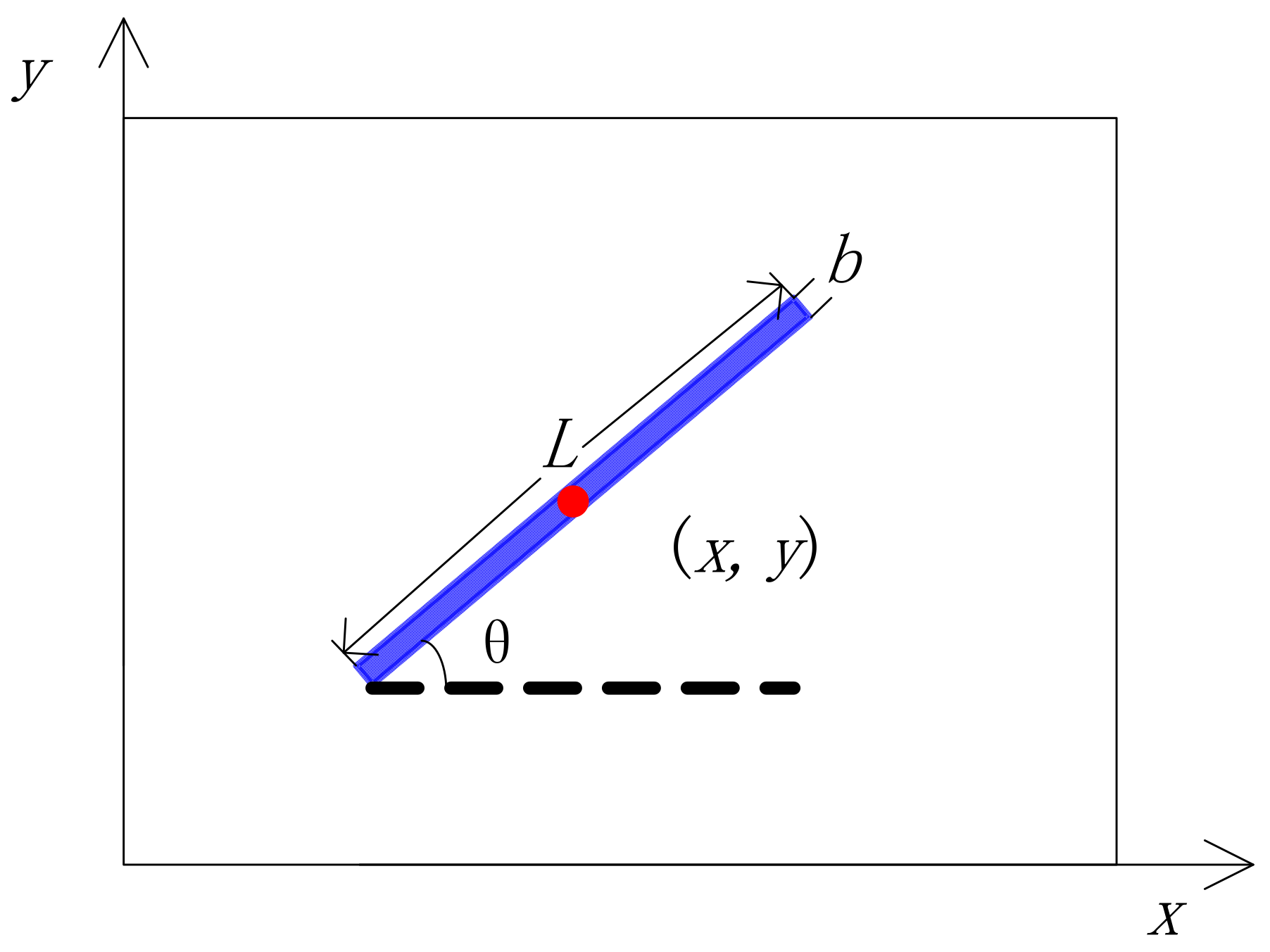
2.2. Physical Model
- (1)
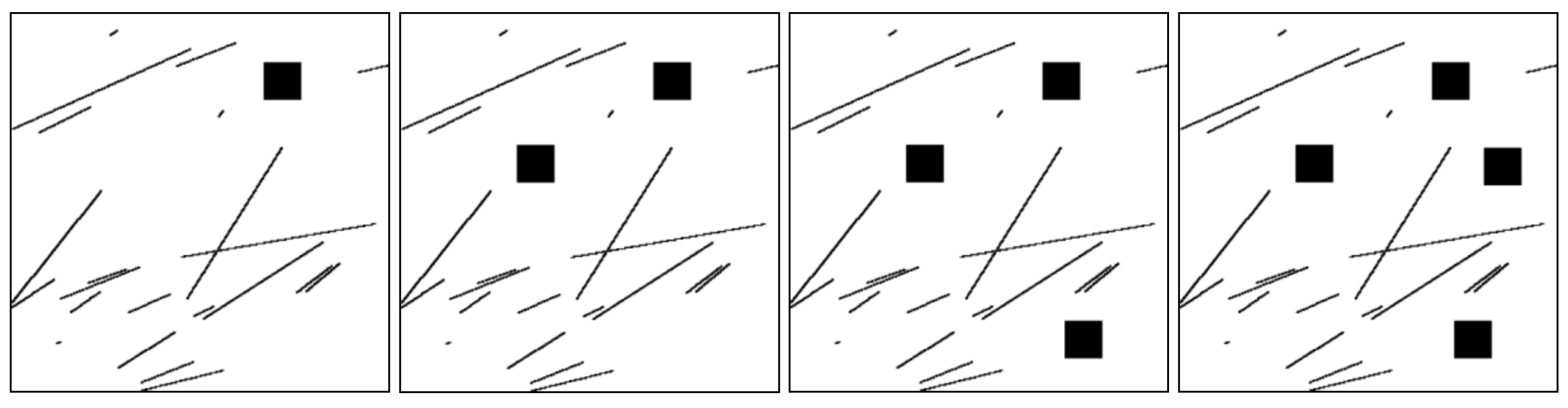
- Physical model I
- (2)
- Physical model II
- (3)
- Physical model III
3. Results and Discussion
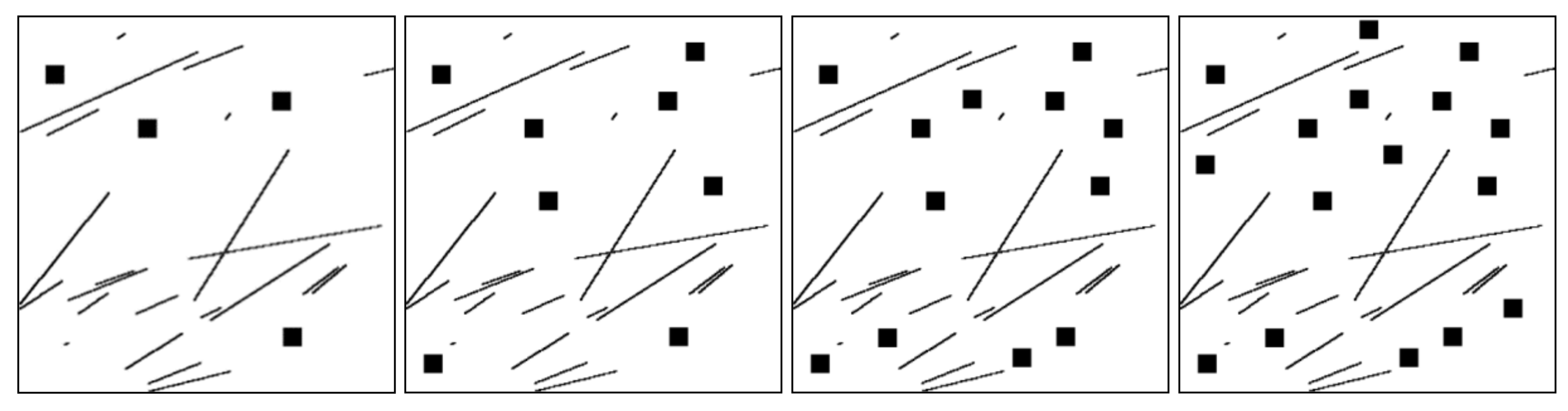
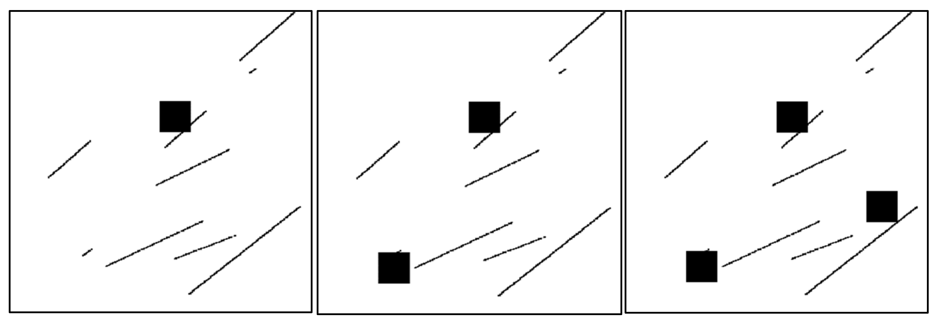
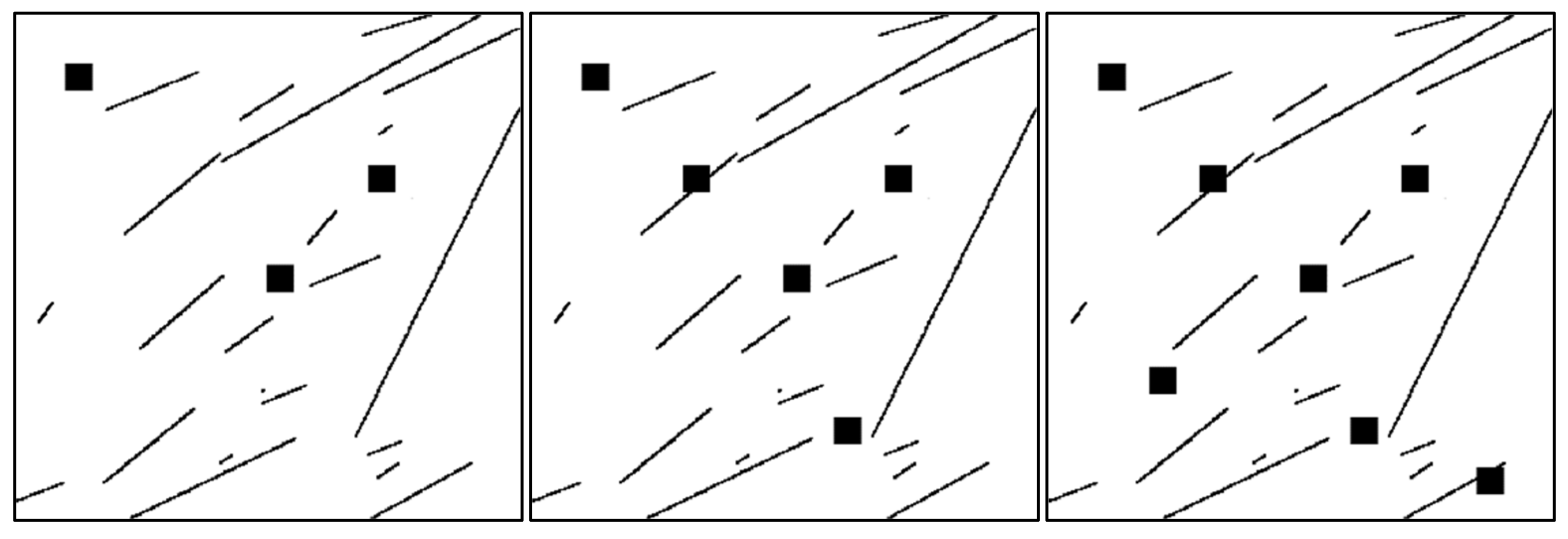
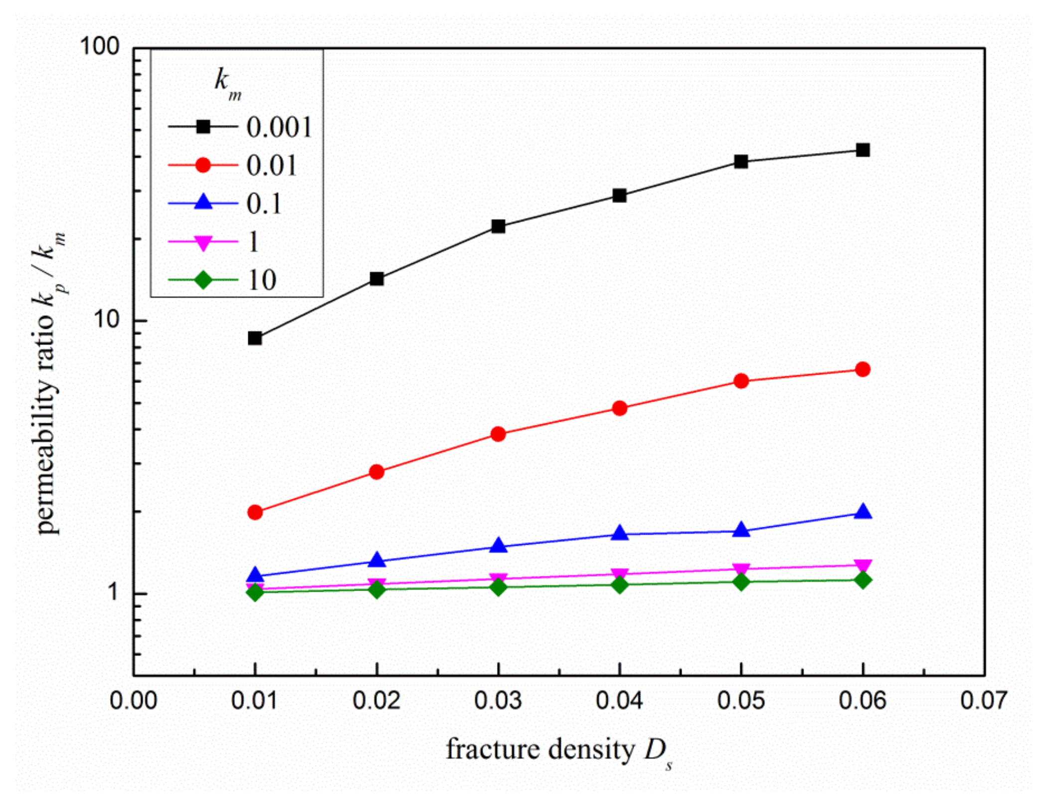
3.1. The Influence of Fracture Density
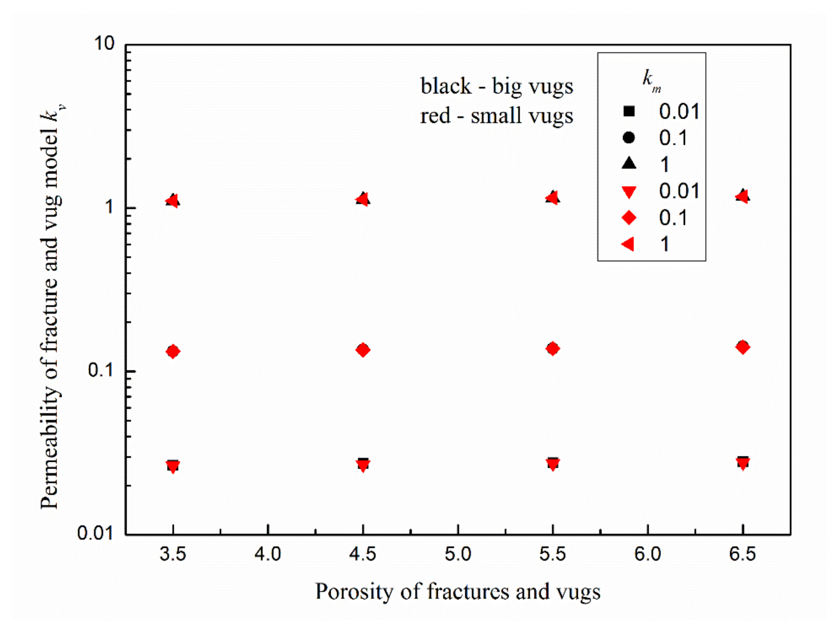
3.2. The Influence of Fractures and Vugs
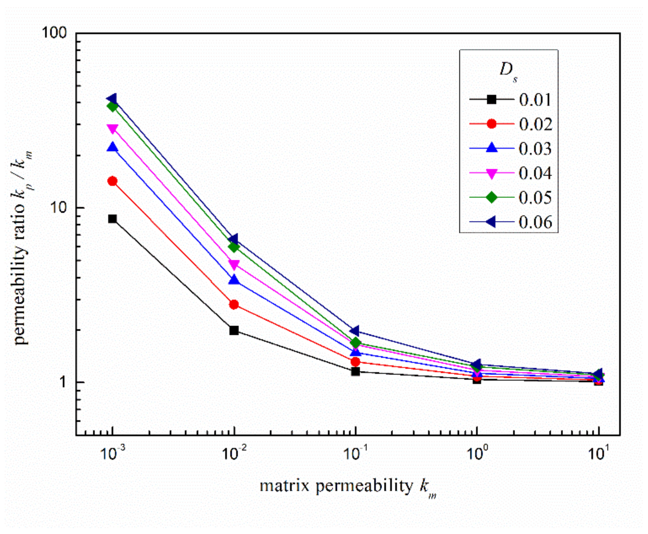
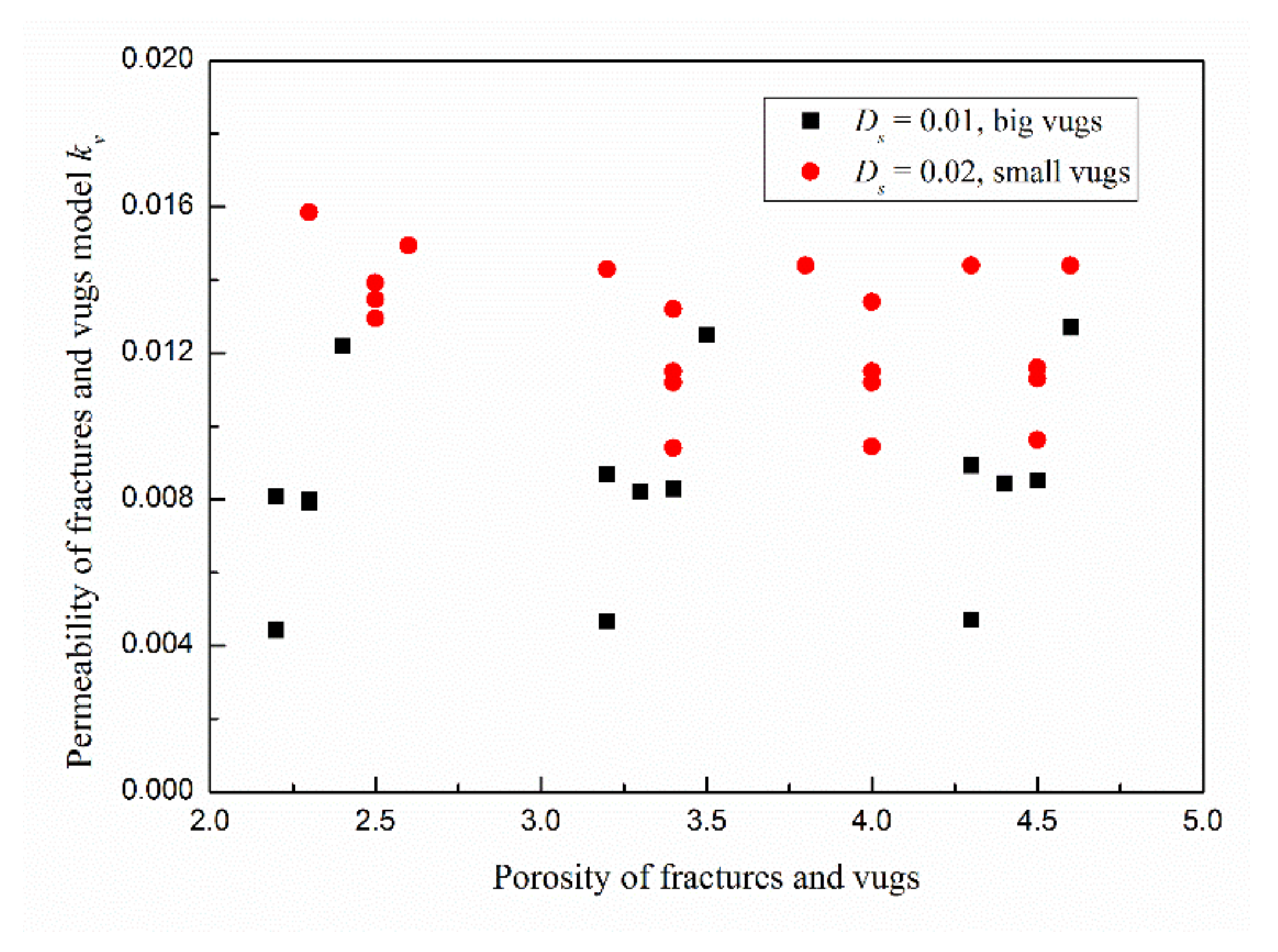
3.3. The Influence of Fracture Density and Vugs Volume
4. Conclusions
Author Contributions
Funding
Institutional Review Board Statement
Informed Consent Statement
Conflicts of Interest
References
- Snow, D.T. Anisotropie Permeability of Fractured Media. Water Resour. Res. 1969, 5, 1273–1289. [Google Scholar] [CrossRef]
- Lough, M.; Lee, S.; Kamath, J. An Efficient Boundary Integral Formulation for Flow Through Fractured Porous Media. J. Comput. Phys. 1998, 143, 462–483. [Google Scholar] [CrossRef]
- Teimoori, A.; Supervisor, S.; Rahman, S.S. Calculation of the Effective Permeability and Simulation of Fluid Flow in Naturally Fractured Reservoirs. Ph.D. Thesis, University of New South Wales, Sydney, Australia, 2005. [Google Scholar]
- Liu, R.; Jiang, Y.; Huang, N.; Sugimoto, S. Hydraulic properties of 3D crossed rock fractures by considering anisotropic aperture distributions Citation. Adv. Geo-Energy Res. 2018, 2, 113–121. [Google Scholar] [CrossRef] [Green Version]
- Ijeje, J.J.; Gan, Q.; Cai, J. Influence of permeability anisotropy on heat transfer and permeability evolution in geothermal reservoir. Adv. Geo-Energy Res. 2019, 3, 43–51. [Google Scholar] [CrossRef]
- Chen, J.; Wang, L.; Wang, C.; Yao, B.; Tian, Y.; Wu, Y.-S. Automatic fracture optimization for shale gas reservoirs based on gradient descent method and reservoir simulation. Adv. Geo-Energy Res. 2021, 5, 191–201. [Google Scholar] [CrossRef]
- Zhang, L.; Kang, Q.; Yao, J.; Gao, Y.; Sun, Z.; Liu, H.; Valocchi, A. Pore scale simulation of liquid and gas two-phase flow based on digital core technology. Sci. China Ser. E Technol. Sci. 2015, 58, 1375–1384. [Google Scholar] [CrossRef]
- Cui, R.; Feng, Q.; Chen, H.; Zhang, W.; Wang, S. Multiscale random pore network modeling of oil-water two-phase slip flow in shale matrix. J. Pet. Sci. Eng. 2019, 175, 46–59. [Google Scholar] [CrossRef]
- Blunt, M.; King, P. Relative permeabilities from two- and three-dimensional pore-scale network modelling. Transp. Porous Media 1991, 6, 407–433. [Google Scholar] [CrossRef]
- Wang, H.; Yuan, X.; Liang, H.; Chai, Z.; Shi, B. A brief review of the phase-field-based lattice Boltzmann method for multiphase flows. Capilarity 2019, 2, 33–52. [Google Scholar] [CrossRef] [Green Version]
- Osher, S.; Sethian, J.A. Fronts propagating with curvature-dependent speed: Algorithms based on Hamilton-Jacobi formulations. J. Comput. Phys. 1988, 79, 12–49. [Google Scholar] [CrossRef] [Green Version]
- Hirt, C.W.; Nichols, B.D. Volume of fluid (VOF) method for the dynamics of free boundaries. J. Comput. Phys. 1981, 39, 201–225. [Google Scholar] [CrossRef]
- Zhu, G.; Kou, J.; Yao, B.; Wu, Y.-S.; Yao, J.; Sun, S. Thermodynamically consistent modelling of two-phase flows with moving contact line and soluble surfactants. J. Fluid Mech. 2019, 879, 327–359. [Google Scholar] [CrossRef] [Green Version]
- Zhang, L.; Xu, C.; Guo, Y.; Zhu, G.; Cai, S.; Wang, X.; Jing, W.; Sun, H.; Yang, Y.; Yao, J. The Effect of Surface Roughness on Immiscible Displacement Using Pore Scale Simulation. Transp. Porous Media 2021. [Google Scholar] [CrossRef]
- Zhu, G.; Kou, J.; Yao, J.; Li, A.; Sun, S. A phase-field moving contact line model with soluble surfactants. J. Comput. Phys. 2020, 405, 109170. [Google Scholar] [CrossRef]
- Yang, Y.; Tao, L.; Yang, H.; Iglauer, S.; Wang, X.; Askari, R.; Yao, J.; Zhang, K.; Zhang, L.; Sun, H. Stress Sensitivity of Fractured and Vuggy Carbonate: An X-Ray Computed Tomography Analysis. J. Geophys. Res. Solid Earth 2020, 125, e2019JB018759. [Google Scholar] [CrossRef]
- Cai, S.; Zhang, L.; Kang, L.; Yang, Y.; Jing, W.; Zhang, L.; Xu, C.; Sun, H.; Sajjadi, M. Spontaneous Imbibition in a Fractal Network Model with Different Wettabilities. Water 2021, 13, 2370. [Google Scholar] [CrossRef]
- Chen, X.; Mohanty, K.K. Pore-scale mechanisms of immiscible and miscible gas injection in fractured carbonates. Fuel 2020, 275, 117909. [Google Scholar] [CrossRef]
- Wang, Z.; Fan, W.; Sun, H.; Yao, J.; Zhu, G.; Zhang, L.; Yang, Y. Multiscale flow simulation of shale oil considering hydro-thermal process. Appl. Therm. Eng. 2020, 177, 115428. [Google Scholar] [CrossRef]
- Li, Q.; Liu, D.; Cai, Y.; Zhao, B.; Lu, Y.; Zhou, Y. Effects of natural micro-fracture morphology, temperature and pressure on fluid flow in coals through fractal theory combined with lattice Boltzmann method. Fuel 2021, 286, 119468. [Google Scholar] [CrossRef]
- Broadwell, J.E. Shock Structure in a Simple Discrete Velocity Gas. Phys. Fluids 1964, 7, 1243. [Google Scholar] [CrossRef]
- Hardy, J.; De Pazzis, O.; Pomeau, Y. Molecular dynamics of a classical lattice gas: Transport properties and time correlation functions. Phys. Rev. A 1976, 13, 1949–1961. [Google Scholar] [CrossRef]
- McNamara, G.R.; Zanetti, G. Use of the Boltzmann Equation to Simulate Lattice-Gas Automata. Phys. Rev. Lett. 1988, 61, 2332–2335. [Google Scholar] [CrossRef]
- Higuera, F.J.; Jimenez, J. Boltzmann Approach to Lattice Gas Simulations. EPL Europhys. Lett. 1989, 9, 663–668. [Google Scholar] [CrossRef]
- Chen, S.; Chen, H.; Martnez, D.; Matthaeus, W. Lattice Boltzmann model for simulation of magnetohydrodynamics. Phys. Rev. Lett. 1991, 67, 3776–3779. [Google Scholar] [CrossRef]
- Grunau, D.; Chen, S.; Eggert, K. A lattice Boltzmann model for multiphase fluid flows. Phys. Fluids A Fluid Dyn. 1993, 5, 2557–2562. [Google Scholar] [CrossRef] [Green Version]
- Spaid, M.A.A.; Lattice, F.R.P., Jr. Boltzmann methods for modeling microscale flow in fibrous porous media. Phys. Fluids 1997, 9, 2468–2474. [Google Scholar] [CrossRef]
- Freed, D.M. Lattice-Boltzmann Method for Macroscopic Porous Media Modeling. Int. J. Mod. Phys. C 1998, 9, 1491–1503. [Google Scholar] [CrossRef]
- Guo, Z.; Zhao, T.S. Lattice Boltzmann model for incompressible flows through porous media. Phys. Rev. E 2002, 66, 036304. [Google Scholar] [CrossRef]
- Kang, Q.; Zhang, D.; Chen, S. Unified lattice Boltzmann method for flow in multiscale porous media. Phys. Rev. E 2002, 66, 056307. [Google Scholar] [CrossRef] [Green Version]
- Chen, S.; Doolen, G.D. LATTICE BOLTZMANN METHOD FOR FLUID FLOWS. Annu. Rev. Fluid Mech. 1998, 30, 329–364. [Google Scholar] [CrossRef] [Green Version]
- Zhang, L.; Kang, Q.; Chen, L.; Yao, J. Simulation of Flow in Multi-Scale Porous Media Using the Lattice Boltzmann Method on Quadtree Grids. Commun. Comput. Phys. 2016, 19, 998–1014. [Google Scholar] [CrossRef]
- Qian, Y.H.; D’Humières, D.; Lallemand, P. Lattice BGK Models for Navier-Stokes Equation. EPL Europhys. Lett. 1992, 17, 479–484. [Google Scholar] [CrossRef]
- Zeng, Q.; Yao, J. Numerical simulation of fracture network generation in naturally fractured reservoirs. J. Nat. Gas Sci. Eng. 2016, 30, 430–443. [Google Scholar] [CrossRef]
- Zou, Q.; He, X. On pressure and velocity boundary conditions for the lattice Boltzmann BGK model. Phys. Fluids 1997, 9, 1591–1598. [Google Scholar] [CrossRef] [Green Version]


Publisher’s Note: MDPI stays neutral with regard to jurisdictional claims in published maps and institutional affiliations. |
© 2021 by the authors. Licensee MDPI, Basel, Switzerland. This article is an open access article distributed under the terms and conditions of the Creative Commons Attribution (CC BY) license (https://creativecommons.org/licenses/by/4.0/).
Share and Cite
Zhang, L.; Ping, J.; Shu, P.; Xu, C.; Li, A.; Zeng, Q.; Liu, P.; Sun, H.; Yang, Y.; Yao, J. The Influence of Fracture on the Permeability of Carbonate Reservoir Formation Using Lattice Boltzmann Method. Water 2021, 13, 3162. https://doi.org/10.3390/w13223162
Zhang L, Ping J, Shu P, Xu C, Li A, Zeng Q, Liu P, Sun H, Yang Y, Yao J. The Influence of Fracture on the Permeability of Carbonate Reservoir Formation Using Lattice Boltzmann Method. Water. 2021; 13(22):3162. https://doi.org/10.3390/w13223162
Chicago/Turabian StyleZhang, Lei, Jingjing Ping, Pinghua Shu, Chao Xu, Aoyang Li, Qingdong Zeng, Pengfei Liu, Hai Sun, Yongfei Yang, and Jun Yao. 2021. "The Influence of Fracture on the Permeability of Carbonate Reservoir Formation Using Lattice Boltzmann Method" Water 13, no. 22: 3162. https://doi.org/10.3390/w13223162