
Impact of Sediment Layer on Longitudinal Dispersion in Sewer Systems


Institute of Hydrology, Slovak Academy of Sciences, Dúbravská cesta 9, 84104 Bratislava, Slovakia
*
Author to whom correspondence should be addressed.
Water 2021, 13(22), 3168; https://doi.org/10.3390/w13223168
Submission received: 28 September 2021
/
Revised: 25 October 2021
/
Accepted: 2 November 2021
/
Published: 10 November 2021
(This article belongs to the Special Issue Water Quality Modeling and Monitoring)
Abstract
:Experiments focused on pollution transport and dispersion phenomena in conditions of low flow (low water depth and velocities) in sewers with bed sediment and deposits are presented. Such conditions occur very often in sewer pipes during dry weather flows. Experiments were performed in laboratory conditions. To simulate real hydraulic conditions in sewer pipes, sand of fraction 0.6–1.2 mm was placed on the bottom of the pipe. In total, we performed 23 experiments with 4 different thicknesses of sand sediment layers. The first scenario is without sediment, the second is with sediment filling 3.4% of the pipe diameter (sediment layer thickness = 8.5 mm), the third scenario represents sediment filling 10% of the pipe diameter (sediment layer thickness = 25 mm) and sediment fills 14% of the pipe diameter (sediment layer thickness = 35 mm) in the last scenario. For each thickness of the sediment layer, a set of tracer experiments with different flow rates was performed. The discharge ranges were from (0.14–2.5)·10−3 m3·s−1, corresponding to the range of Reynolds number 500–18,000. Results show that in the hydraulic conditions of a circular sewer pipe with the occurrence of sediment and deposits, the value of the longitudinal dispersion coefficient Dx decreases almost linearly with decrease of the flow rate (also with Reynolds number) to a certain limit (inflexion point), which is individual for each particular sediment thickness. Below this limit the value of the dispersion coefficient starts to rise again, together with increasing asymmetricity of the concentration distribution in time, caused by transient (dead) storage zones.
1. Introduction
Transport of substances in flowing water is in principle the result of two basic phenomena: advection and dispersion. Within sewer systems, for example, longitudinal dispersion causes the decrease of pollution concentration and its distribution in time.
Special situations occur very often in real sewer systems at time of low flows during dry weather periods. Flow in such sewer systems can be characterised with specific hydraulic conditions: low discharges (especially during night-time) and sediment and deposit formation. Sediments on the pipe bottom change not only the pipe (streambed) hydraulic roughness, but in cases of the same discharge also cause a reduction in flow depth [1], which leads to flow with low Reynolds numbers, i.e., close to the laminar flow regime. As water quality models assume turbulent flow in general, the modelling of the wastewater quality under such circumstances could be inaccurate. So, there is a need to improve dispersion models with regard to the specific hydraulic conditions in partially filled sewer pipes with free surface flow, respecting real conditions (sediment occurrence).
This paper describes the results of an experimental study with the aim to characterize the dispersion process changes in a pipe flow system with bottom deposits for very low discharges, depths, velocities and corresponding Reynolds numbers. The novelty of this study is that the dispersion process is evaluated in pipes with sediments and deposits, thus simulating real conditions in sewer systems.
The basic objectives defined for our study are:
- To investigate how the sediment occurrence affects the flow and dispersion processes in sewer networks in hydraulic conditions of low discharges, velocities and shallow depth;
- To determine, if under such hydraulic conditions, transient storage zones (dead zones) are formed; and consequently
- Whether the Gaussian approximation (response) function is an appropriate approximation for the dispersion process description under stated hydraulic conditions.
In the past, different authors have dealt with related topics, however with different hydraulic conditions. Taylor’s pioneer works [2,3] presented the dispersion process in pipes, however under the conditions of the pressurized flow in the pipes (no free surface flow). Dispersion in pressurised pipes (water supply systems) for a wider spectrum of flow regimes was a subject of the work of Hart [4], Abokifa [5] and Romero-Gomez [6]. A large set of experiments was evaluated by Rieckermann et al. [7], where 60 different datasets from tracer experiments in different urban systems were analysed for dispersion in conditions of low flows during dry periods. However, as the authors of this study stated, the impacts of biofilm, rain events and sediments on the longitudinal dispersion coefficient could not be evaluated from the experimental database. Hart et al. [8] investigated the longitudinal dispersion in hydraulic conditions of unsteady flow with rapid changes. Guymer [9] and Mark [10] studied the solute transport in surcharged sewer manholes.
Generally, prediction of the rate of pollution spreading is necessary for water quality protection management. Different authors have described various approaches how to better understand the concept of water quality problems and questions [11,12,13,14,15,16]. If an accidental pollution leak into a stream occurs, the prognosis of pollutant transport and spreading is necessary for rapid and effective implementation of the protective measures. In real conditions the dispersion process is affected by several factors, which influence the dispersion process as well as the hydrodynamic parameters [17]. Bottom sediment and deposits, which change flow conditions in general (mainly by changes of streambed form and its roughness), are some of them. Impacts of mentioned factors on the dispersion process can be significant, especially at low flow velocities and water depths, which often occur in sewer pipes under dry weather flows.
2. Theoretical Background
Dispersion is a very complex process. It can be described as a combination of molecular and turbulent diffusion, advection and shear [15]. Dispersion of the solute in flowing water is caused by the non-uniform distribution of velocity resulting from differences in geometry, roughness and kinematics. Progress of the dispersion phenomenon is characterized by dispersion zones as follows: the initial mixing zone, the complete mixing zone and the “far” field zone, where dispersion is considered as longitudinal and in this way as one-dimensional in the flow direction. In mathematical and simulation models, the dispersion rate is expressed by the value of dispersion coefficient. Different evaluation procedures supported by experimental studies have been proposed for determination of this coefficient [18,19].
Spreading and transport of chemically stable substances in flowing water is possible to describe by a one-dimensional advection–dispersion equation (ADE) with the following assumptions:
- Homogenous concentration of substance in vertical and transversal directions, i.e., vertical and lateral dispersion can be neglected;
- The substance is completely soluble in water;
- The substance is conservative (the substance is not subject to chemical or biological processes);
- Quantity of the substance is preserved during the time of transport.
The form of this equation is:
where C is the concentration of substance (kg·m−3), t is the time of transport (s), vx is the longitudinal fluid velocity (m·s−1), Dx is the longitudinal dispersion coefficient (m2 s−1), x is the distance in the longitudinal direction (m) and Ms expresses the substance sources or sinks (kg·m−3 s−1).
An analytical solution of Equation (1) is not simply achievable. It can be gained only for specific cases and with various mathematical approaches and conditions. One of the most used mathematical forms is the general solution of the ADE by Socolofsky and Jirka [20], and eventually by Fischer et al. [12] and Martin, McCutcheon, and Schottman [21]:
where M is the mass of substance instantaneously input to a stream (kg), A is the discharge area of the cross section profile of a stream (m2) and f is the unknown function (“similarity solution”).
The most-used function in the Equation (2), and in this way the most used analytical solution for Equation (1) for simplified conditions and instantaneous solute input, has the form [21,22]:
where u is the flow velocity in x direction (m·s−1).
Equation (3) is often titled by various authors as the “standard solution”. In fact, it represents the Gaussian response function (also used as the term Gaussian approximation function) to the initial impulse, i.e., instantaneous (pulse) input of substance into the stream. Hart [4] considers this function as a good estimation (approximation) of mixing characteristics for turbulent and critical flows.
However, the form of Equation (3) assumes symmetrical spreading of substance up- and downstream (Gauss distribution). It means that the temporary storage zones (dead zones) or other singularities influencing substance spreading and changing the shape of the concentration distribution curve are not taken into account [23]. Use of this approximation in streams with presence of such singularities can be incorrect. As we discovered during our research, the sediments in sewer pipes combined with low discharges form temporary storage (dead) zones.
Mathematical and numerical solutions of dispersion in streams with dead zones are widely known and described in the literature [16,24,25,26], as well as various impacts of hydraulic parameters on the dispersion rate [27,28,29]. However, most of these solutions use complicated mathematical apparatus and their numerical applications [24,25,30,31].
For this reason, an alternative function based on the asymmetrical substance spreading assumption has been used for the 1-D analytic solution of the ADE. This function comes from the Gumbel statistical distribution [32]:
where Dx,G is the longitudinal dispersion coefficient (m2 s−1) used in this Gumbel’s approximation model.
Both the Gaussian approximation model (Equation (3)) and the Gumbel’s approximation model (Equation (4)) are two-parametric models, where the first parameter is the dispersion coefficient and the second parameter is the peak time (mean), expressed through the velocity of water flow u.
Even better results and conformity between models and data from real conditions can be obtained using the three parametric Generalised Extreme Value (GEV) distribution model [32]:
where Dx,GEV is the longitudinal dispersion coefficient (m2 s−1) used in the GEV distribution model and ξ is the so-called shape parameter. This shape parameter expresses the asymmetry of the concentration distribution in time. A “neutral” value of the shape parameter, which corresponds to the shape of the Gaussian approximation function, is −0.288. A lower value than −0.288 of the shape coefficients should not occur. Higher values of this coefficient are caused by dead zones and corresponding asymmetricity of the concentration distribution in time (represented by longer “tails” of the time concentration curves). Higher values of the shape parameter ξ in this way indirectly characterise the extent of dead zones.
It is necessary to mention that the last two approximation models try to describe the dispersion phenomenon numerically and their physical meaning is limited. On the other hand, such an approach corrects the postulate of a symmetrical movement of particles in flow upstream and downstream, which is distorted by the dead zones.
3. Materials and Methods
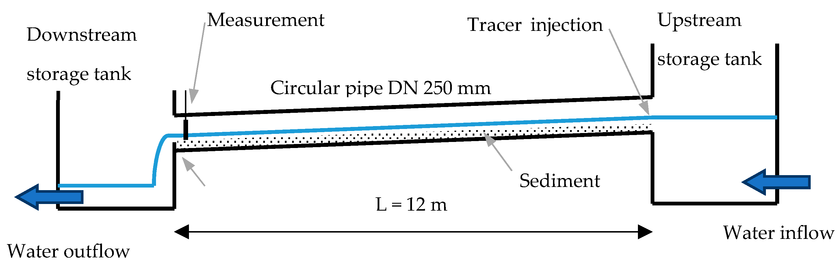
Our experiments were performed in the hydraulic laboratory of the WUT (Warsaw University of Technology, Poland). All laboratory experiments were done in a flume with a circular cross section in the form of a pipe. The length of the pipe was 12 m, its inner diameter was 250 mm, and slope of the pipe was 5‰. Material of the pipe was smooth transparent plastic. There were openings at the top of the pipe in 2 m intervals enabling manipulation with measuring devices inside the pipe as well as the sediment insertion and retrieval.
There was a storage tank at the pipe beginning, from which water flows gravitationally (while maintaining a constant water level) into the circular pipe. Laboratory flume ends by a free outfall to another storage tank with an outlet in the tank bed (Figure 1). In all experiments, the pipe was only partially full, so there was a free water flow (free water surface and water–air interface).
For all experiments, drinking water was used (with no recirculation) and in this way the problem with changes in background concentration was eliminated. Discharge was measured individually for each set of experiments and was regulated with a lever valve.
To create real hydraulic conditions, including the sediments and deposits in sewer pipes, we inserted sand with different granularities and in different layer thicknesses into the pipe. We used a sand of fraction in range 0.6–1.2 mm. To create conditions similar to those in real sewer pipes, we spread rougher material (fine gravel) on the top of the smoother sand layer. The sand and top gravel layer was spread and finely compacted. Prior to the experiments, water flowed through the pipe for about 20 min to saturate the sand layer and to form the surface of the sand layer. After such preparation of the sediment, the sediment layer was fixed and did not move during the experiments. All experiments were performed with fixed sediment, starting with minimal flow rate. The flow rates were stepwise increased, until a movement of sediment (erosion) was observed. After this, the experiments were stopped to prevent the wash-out of the sediment layer.
Water depth was measured with a special contact gauge. Such measurements proved to be relatively inaccurate due to problems with determining the sediment–water interface as well as the flow disintegration and forming of flow with different depths across the pipe width (dead zones forming). Because of this, the water depths, given in the text below, are values numerically derived from the hydraulic parameters (discharge/flow width). These values correspond with the physically measured water depth values.
We performed 4 sets of experiments with different layer thicknesses. The first set of experiments was performed with the sediment layer of 0 mm (no sediments), then 3.4% of the pipe diameter was filled with sand sediment (layer thickness = 8.5 mm). The next sets were done with 10% and 14% sediment filling of the pipe diameter (layer thickness = 25 mm and 35 mm, respectively). For each sand layer thickness, a set of tracer experiments was done with different flow rates ranging from 0.14 L·s−1 up to 2.5 L·s−1. The limit value of the maximum flow rate used during experiments was determined for each set of experiments individually with respect to to the sand wash-out.
Tracer experiments were performed using Rhodamine WT and kitchen salt (sodium chloride, NaCl) as tracers. The tracer mixture was prepared by adding 1 kg salt (mixed and completely dissolved in water) and 0.05 mL of the Rhodamine WT tracer (20% solution) into 10 L water. For each experiment, 0.1 L of this solution mixture was used. For the measurement of concentration distribution in time, we used a fluorometric and a conductivity probe placed at the pipe end, approximately 200 mm before its end. Tracers were discharged instantaneously and manually at the inlet of pipeline from the upstream storage tank.
Each tracer experiment (grouping different discharges and layer thicknesses) was redone five times. Data with 1 s step were recorded electronically and digitally in the storage unit of the corresponding gauge.
It is worth mentioning that in the consequent evaluation process we used only the measured data from the fluorometric probe, because we found that this probe responded quicker to the concentration changes. Its response time was almost imperceptible, while the response of conductivity probe was about 2–3 s, so values measured by the conductivity probe were probably time-averaged by the device software.
4. Results
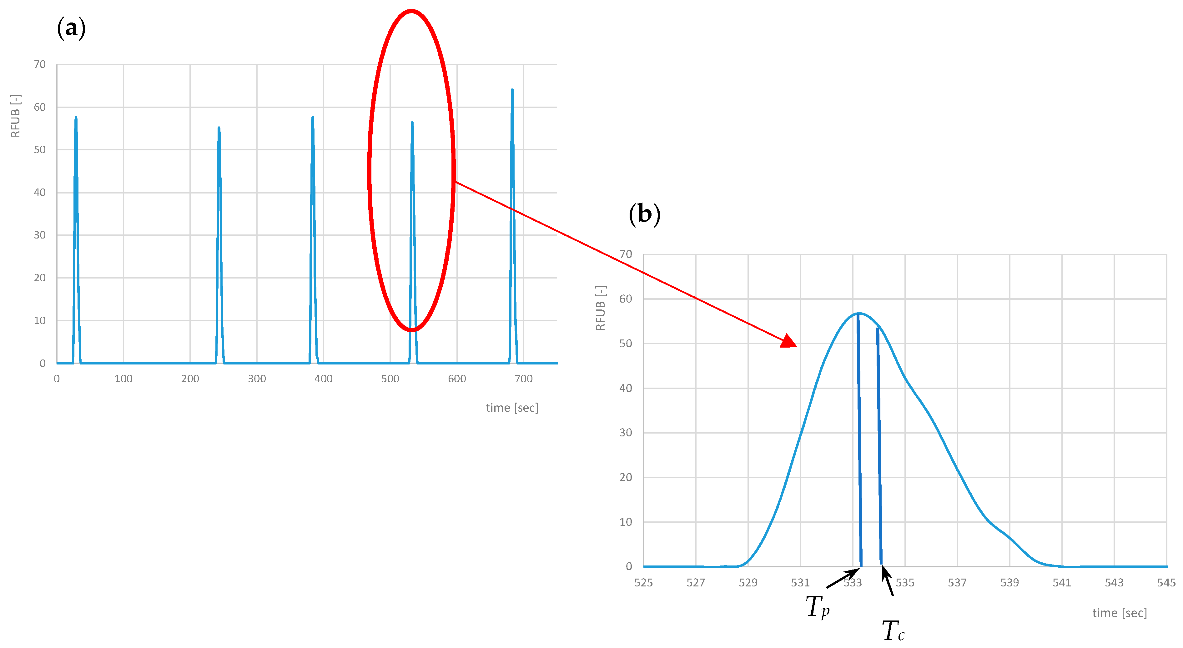
One dataset was created by five tracer experiments that were performed with the same flow rate and sand layer thickness. Figure 2 illustrates an example of such a dataset. In total, 23 tests were conducted with flow rate range from 0.14 L·s−1 up to 2.5 L·s−1 and Reynold’s number ranging from 467 up to 18,463.
The flow velocity in particular experiments was determined based on the characteristic concentration distribution points, according to Li, Abrahams, and Atkinson [33] and Elder [34]. For each experiment, the characteristic times were determined, namely the peak time Tp and the centroid time Tc (see Figure 2). Corresponding velocities were set up based on the circular pipe length and by the corresponding time, i.e., up = L/Tp, uc = L/Tc. The peak velocity up was used for the dispersion coefficient evaluation according to Equations (3)–(5) and the centroid velocity uc was used for determination of all other parameters (e.g., the Reynolds number Re).
To determine the dispersion parameters, each measured tracer experiment was evaluated according to Equations (3)–(5). A statistical approach was used for evaluation of the results. The optimal set of dispersion parameters is determined by the best approximation between measured and modelled data. This was achieved by finding the minimal root square mean error (RMSE). For the numeric optimisation procedure, the function Solver built into the MS Excel environment was used.
All values of parameters determined from five tracer experiments were averaged. An example of raw data and averaged (approximated by Equations (3)–(5) data is shown in Figure 3. Data in this figure are normalised, i.e., concentration with respect to the maximum (peak) concentration cmax and the time axis with respect to the time, corresponding to the peak concentration tc,max.
It is difficult to determine the total measurement uncertainty because of the partial uncertainties (e.g., particular devices, flow rate, concentration, timing uncertainty). The overall measurement uncertainty can be estimated by the standard deviation of particular results evaluating all experiments. The average normalised standard deviation for the peak concentrations was 4.68%, for the peak time 1.04% and for the Dx determination about 5.3% (Gauss 5.3%, Gumbel 5.2% and GEV approximation 5.4%).
The complete averaged results for each dataset are summarized in Table 1. The Reynolds number was calculated according to Rapp [35]:
where ρ is the water density (kg·m−3), η is the dynamic viscosity of water (Pa·s), ν = η/ρ is the kinematic viscosity of water (m2·s−1) and d is the characteristic dimension (m). Generally, in the free surface flow theory, as the characteristic dimension can be used: the depth [36], hydraulic radius [37], water depth or the smallest channel dimension [35]. For our calculations, the hydraulic radius was used.
For more detailed specification of the experiment results this table also shows the Péclet’s number, which is defined as
where Pe is the Péclet’s number (-), uc is the water flow velocity (m·s−1), R is the hydraulic radius (m) and Dx (Dx, GEV, respectively) is the longitudinal dispersion coefficient (m2 s−1). The Péclet’s number shows the ratio of advective to diffusive transport in fact. The values of Pe in the Table 1 are calculated with the Gaussian dispersion coefficient value according to Equation (3).
Another parameter listed in the Table 1 is the dimensionless dispersion coefficient Dx,d[-]. This coefficient is defined by [4]
where Dx (Dx, GEV, respectively) is the longitudinal dispersion coefficient (m2 s−1), d is a characteristic dimension (m); in general, the hydraulic radius R (m) can be used as a characteristic dimension, uc is the flow velocity, based on centroid time (m·s−1).
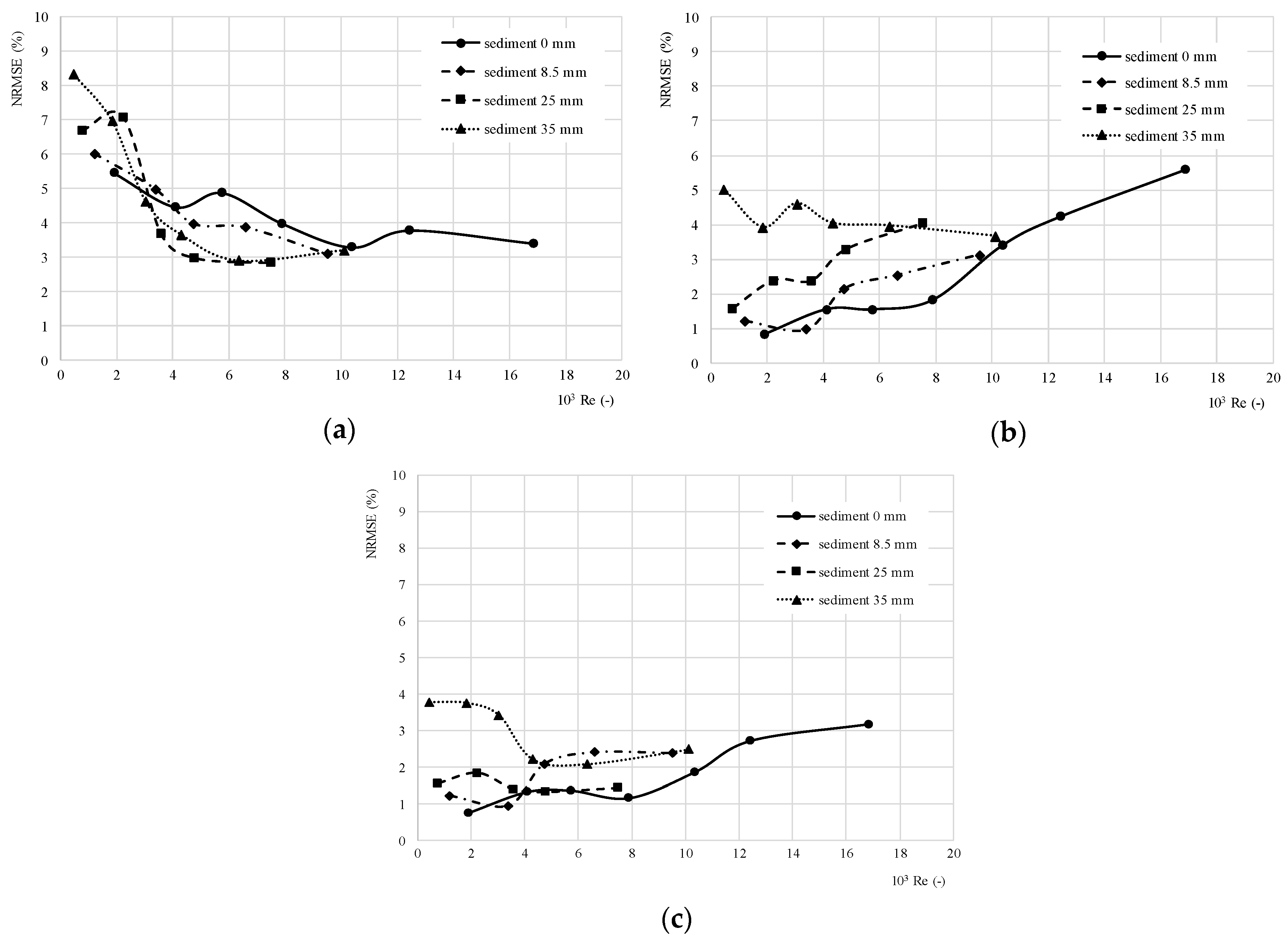
The fit between the measured values and the particular approximation functions (Gauss, Gumbel, GEV approximation functions) was evaluated using standard statistical method root mean square error (RMSE) and the normalised RMSE (NRMSE). The NRMSE values were in range 0.77–7.06%, whereas the average NRMSE value for the Gauss approximation function (Equation (3)) was 4.45%, for the Gumbel approximation function (Equation (4)) 3.03% and for the GEV approximation function (Equation (5)) 2.10%.
The NRMSE columns in the Table 1 documents the root mean square errors for particular approximation methods (Gaussian, Gumbel and GEV). The normalised root mean square errors (RMSE) according to particular approximation methods in this table are also graphically shown in Figure 4.
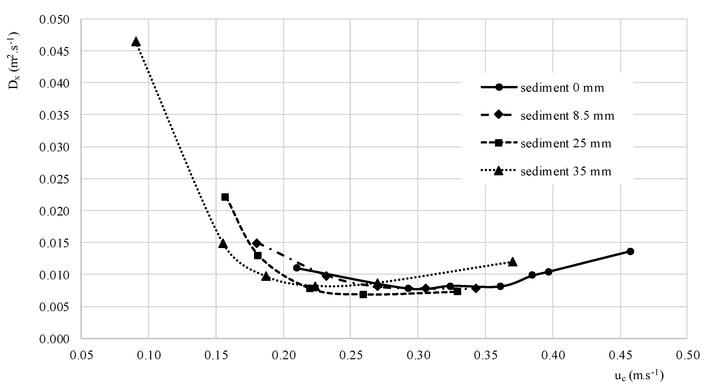
Graphical presentation and evaluation of relations between dispersion coefficient and basic hydraulic parameters (flow velocity and Reynolds number) on the basis of results of the experiments are shown in Figure 5, Figure 6 and Figure 7.
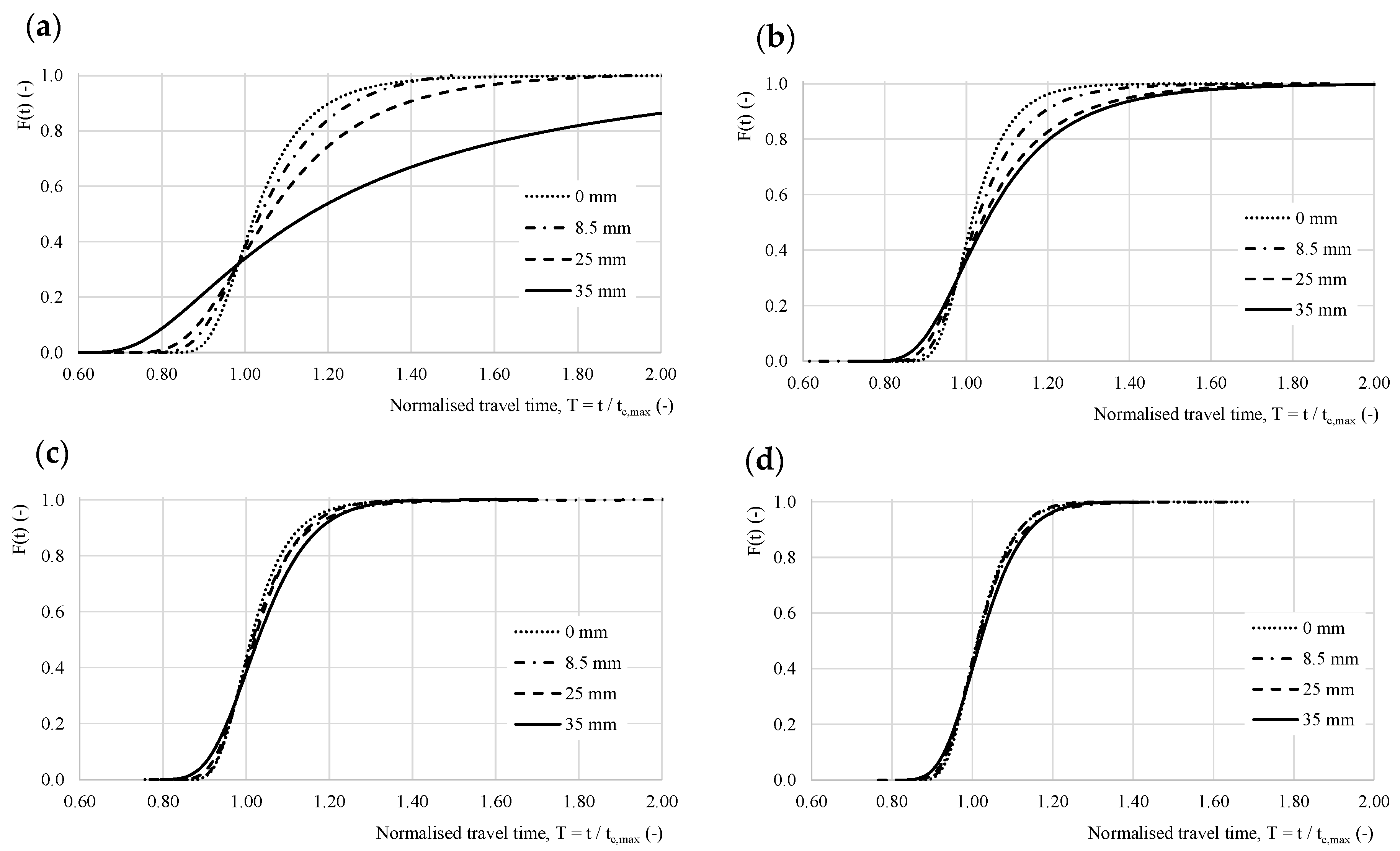
Illustration of the sediment impact on the dispersion process and its parameters is documented on following figures. The cumulative mixing response is documented in Figure 8 in form of the cumulative residence time distribution (CRTD). The displayed curves represent the statistically processed and averaged approximations for particular experiments.
Evaluation of the data showed that the GEV approximation (Equation (5)) is significantly more accurate than the Gaussian approximation (Equation (3)), which is documented in Figure 4. Therefore, in Figure 8 are results evaluated by the GEV approximation. For better illustration, the curves are divided into four groups according to hydraulic conditions, i.e., with similar discharge and corresponding flow velocity. The particular experiment groups, i.e., cases (a)–(d) and corresponding parameters are defined in Table 2. Similarly, as mentioned earlier, also in this Figure (Figure 8) the data are normalised—dimensionless cumulative mass fraction considering to the total tracer mass and the time axis with respect to the time, corresponding to the peak concentration (tc,max).
The dimensionless cumulative mass fraction is defined as
where F(t) is the dimensionless cumulative mass fraction (-), c is the substance concentration (kg·m−3), Q is the flow rate (m3·s−1).
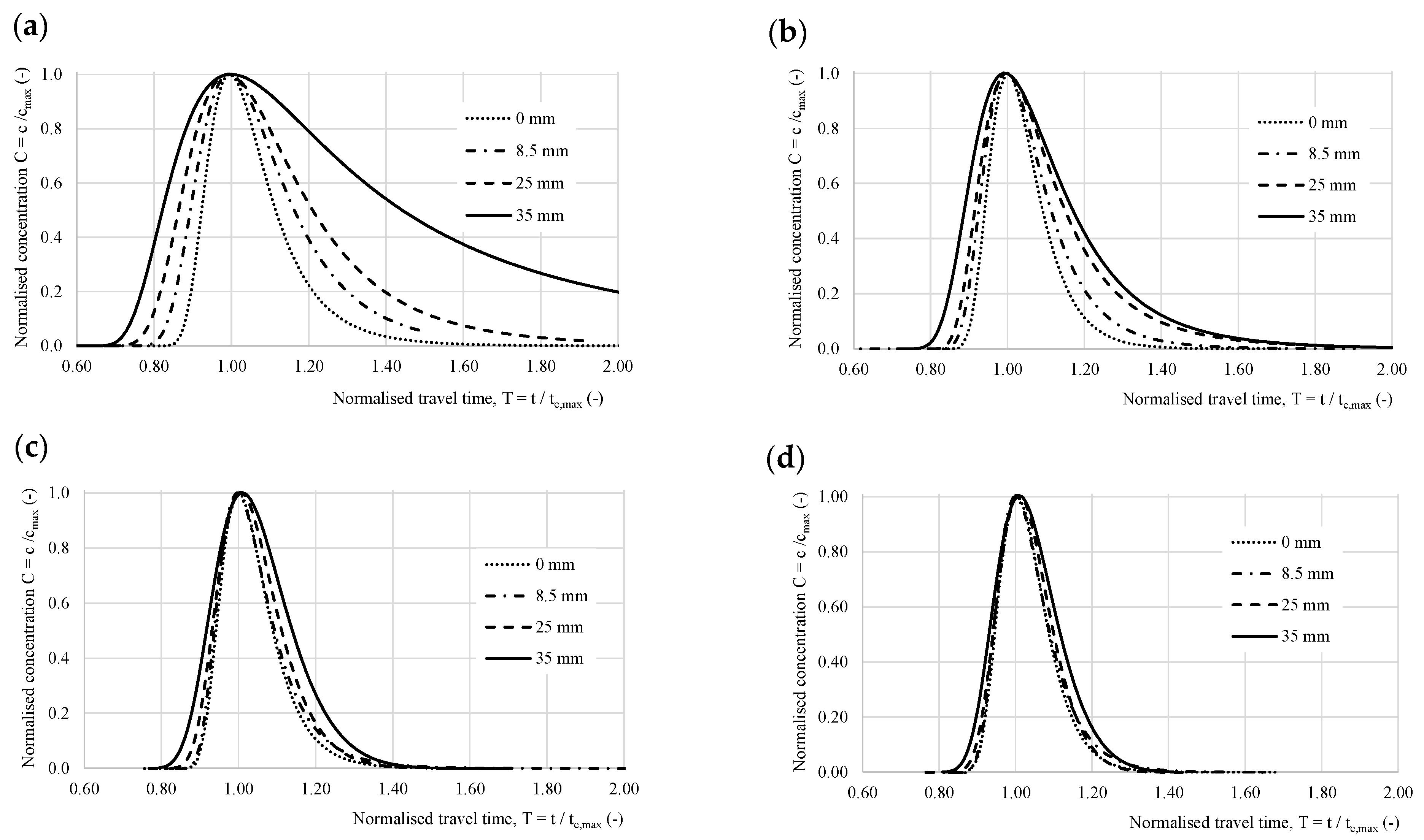
The normalised concentration distributions in time for the experiment groups, as defined in Table 2, are shown in Figure 9. The concentration was normalised similar as in Figure 3.
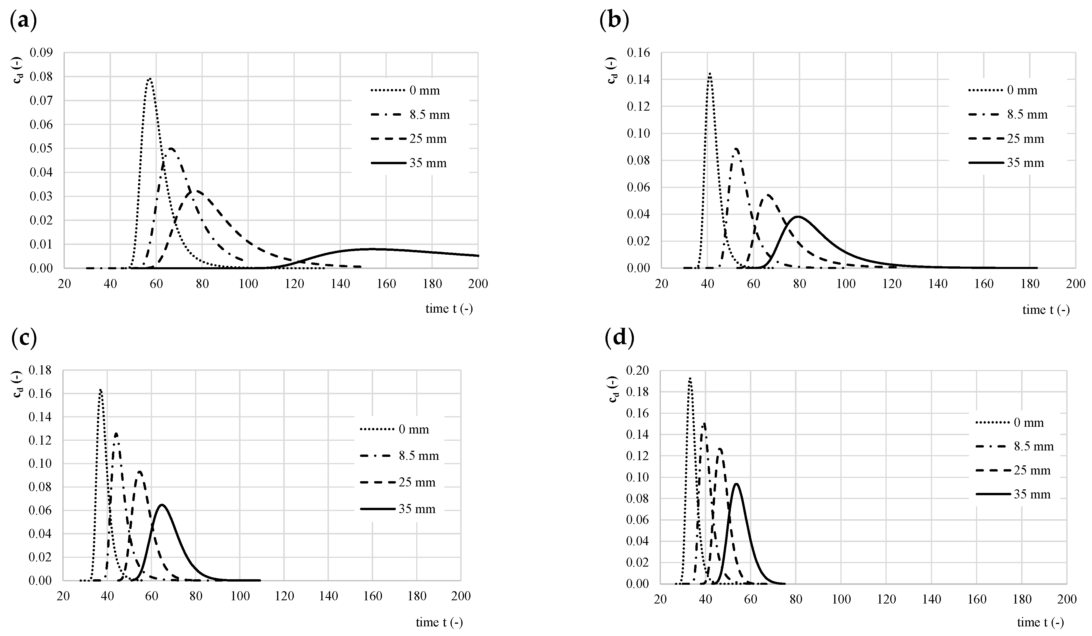
Further graphical documentation of the experiment results is shown in Figure 10. In this case the experiment groups (a)–(d) are also divided according to Table 2. Mass normalisation was used, i.e., in all cases the total tracer mass corresponds to one dimensionless unit; the time is not normalised. The dimensionless mass normalised concentration is defined as
where cd (t) is the dimensionless mass normalised concentration (-), c (t) is the substance concentration in time t (kg·m−3), Q is the flow rate (m3·s−1).
As a supplement of this study and for practical use of the results of all these experiments, we created an approximation equation, which makes it possible to predict or estimate the value of the dimensionless dispersion coefficient Dx,d (-) for use with the Gaussian approximation function (Equation (3)) on the basis of the Re values and the proportion of the sediment layer thickness and pipe diameter:
where ts is the sediment layer thickness (m) and dp is the pipe diameter (m).
A similar approximation equation was created for the use with the Gumbel’s approximation function (Equation (4)):
The Dx,d approximation according to Equations (11) and (12) can be used within the range of our experiments, i.e., in the range of Reynolds number from 400 up to 16,000 and for the ratio of the sediment layer thickness related to the pipe diameter from zero (no sediment) up to 0.14. The normalised root mean square error (NRMSE) between the values of the proposed approximation equation (Equation (11)) and our experiment results for the Gaussian approximation function is 0.37%, the correlation coefficient between both datasets is very close to 1 (R = 0.99984). An example of the approximation equation result is presented in Figure 11. For the Gumbel approximation function, the NRMSE is 0.26% and the correlation coefficient between both datasets is R = 0.99993.
As shown in Table 1, both values are very similar, almost identical. During our research we found a linear dependency between both dispersion coefficients in form Dx,GEV = 1.059 Dx,G − 0.0007 with correlation coefficient R2 = 0.9983. This is probably due to the fact that the Gumbel distribution is a particular case of the GEV distribution. For this reason, the value of the dispersion coefficient Dx,GEV (GEV approximation function) can be used as a substitution for the value of the dispersion coefficient Dx,G (Gumbel approximation function).
The prediction of the shape parameter ξ is very uncertain, because this parameter is expressing the extent of dead zones, so it is difficult to quantify and to estimate this parameter in advance. However, in our research we found a dependence of this shape parameter ξ on the Reynold’s number (Re) in form ξ = 3.88 × Re−0.318 − 0.354 (correlation coefficient R2 = 0.801).
5. Discussion
In this part of our study, we will try to answer to the objectives defined in the introductory part of this paper.
The first issue discussed here should be the question as to whether the laboratory results are influenced by the initial mixing zone. Based on the description of the lab experimental device, it is clear that we used only one concentration measuring device located at the end of the flume. Thus, the total flume length, in which the tracer dispersion took place, also includes the initial mixing zone, where the longitudinal mixing process was affected by the vertical and lateral mixing. However, the measurement sensors were deployed out of the initial mixing zone.
Differences between experiments with and without an initial mixing zone can be found in the literature. Rieckermann [7] describes set of experiments focused on the determination of the dispersion coefficient in sewer networks at the time of low flows during dry weather periods. There were two types of experiments—with initial mixing zone (referred as the type 0–2) and without initial mixing zone (referred as the type 1–2). Authors of the mentioned paper found average relative deviation between both types of experiments −12% with no apparent bias and conclude that the estimated dispersion coefficients of both methods are considered equivalent and the impact of the initial zone can be neglected. On the other hand, it must be acknowledged that the distances and travel times were significantly greater compared with our lab experiments. Based on the visual observation (the flume was made from transparent plastics), the initial zones in flume without sediments was very short, up to 150 mm. In the case of the experiments with sediments, the vertical mixing was very fast because of the small water depths; lateral mixing took place on a longer length, approx. 200–300 mm. As stated below, a problem in the lateral mixing was the disintegration of the coherent fluid flow to smaller streams due to the sediment surface irregularities.
The goal of our research was not to determine the absolute or accurate value of the dispersion coefficient, but study, describe and quantify the sediment impact on the dispersion process in sewers. Because of this, the degree of uncertainty and possible errors influenced all experiments (with and without sediments) in the same way but it did not affect the mutual comparison of the particular experiment results. On the other hand, the results and range of the longitudinal dispersion coefficient values (and also Equation (11)) obtained from these experiments are useable within the range of conditions in which they were performed.
The first objective was to investigate how the sediments affect the flow and dispersion processes in a sewer network in hydraulic conditions of small discharges, velocities and shallow depths. As shown in Figure 5, the value of the dispersion coefficient decreases concurrently as the flow velocity and flow rate decreases. However, this applies until a certain flow velocity is reached and further velocity decrease causes increase of the dispersion coefficient. The inflexion (turning) point in our experiments occurred at velocities ranging from 0.2 to 0.3 m·s−1, more generally expressed in the Reynold number range from 4000 up to 6000 (see Figure 6).
We assume that this phenomenon results from specific hydrodynamic flow conditions, which are caused by shallow water depths and by the irregularities of the sediment surface (even though the surface prior the experiments was carefully trimmed and levelled, during the experiments the sediment smooth surface was slightly eroded by water flow). In extreme cases, if the water depth is smaller than the sediment surface irregularities, the flow can be disintegrated into several smaller streams (bifurcation). This flow disintegration causes high differences of velocity distribution in the cross section profile (the velocity zone near the sediment top impacts the vertical velocity profile; transversal velocity profile is highly irregular due to sediment surface irregularities).
As mentioned above, the sand sediment was trimmed carefully, but before the experiments water was flowing for approx. 20 min to saturate the sand and form the surface level of sediment; so, the irregularities are part of a natural process. It is reasonable to assume that the same process takes place in real sewers. In such cases, the results of dispersion experiments depend on the character of the sediment top layer; they could be very variable and depend on the roughness, thus on the sediment composition and form [38,39]. The character of the sediment top is also subject to temporary changes. In a combined sewer system, the sediment could be washed out during the rain events; in contrast, in dry weather seasons the sediment layer is build-up as the top layer is formed. In real sewer environments, the top layer is formed from organic material and bacterial biofilm and its amount decreases with increasing shear stress [40]. Due to the proportion of fine sediments and biofilm on the surface and their hydraulic conductivity [41], we can assume that no significant subsurface (hyporheic) flow will be formed in the sediments, so the subsurface flow does not form a significant proportion of dead zones.
The second objective was to determine, if under such hydraulic conditions, transient storage zones (dead zones) are formed. The flow disintegration and forming of flow with different depths make conditions for creation of dead zones. This can be stated based on the experimental results presented in Figure 8 and Figure 9.
CRTD curve shape differences in Figure 8 and Figure 9 clearly demonstrate this. A typical feature of dead zones, the asymmetrical shape of the curves, is especially visible in the case of small flow velocities in Figure 8a and Figure 9a. However, in the experiment group with very low discharges, group (a), the curves are more “flat” and can be characterised as similar to the “complete mixing” or “dead water” cases, as described by Danckwerts [42]. With increasing discharges, cases (b)–(d), the differences become smaller and curves become closer to the case of “piston flow with some longitudinal mixing” [42].
Similar characterisation can also be applied for the experiment groups shown in Figure 9. Discharge decrease causes the normalised concentration distributions which in time become “flatter” with longer “tail” (case (a)), whereas the curves for higher discharges are “steeper” with quick increase and decrease of the concentrations (cases (b)–(d).
The ratio of dead zones to the active flow zones and in this way also the impact of dead zones increases with decreasing flow rate and increasing sediment thickness. The cause for this is that the water depth decrease makes the area of active zones smaller, whereas the area of dead zones stays approximately the same. Thus, the ratio between the active and passive (dead) zones is decreasing and dead zones start to significantly influence the dispersion process.
The consequent question is whether the Gaussian approximation function is an appropriate approximation for the dispersion process description under stated hydraulic conditions. To evaluate the measured data, the root mean square error (RMSE) between measured values of tracer concentration and concentration modelled by empirical solutions of ADE was evaluated for each experiment and averaged for particular experiment sets. For these purposes, we evaluated the match of the measured data with the Gaussian approximation function according to Equation (3) and the GEV approximation according to Equation (5). Data from the Gumbel’s approximation by Equation (4) were very similar to the GEV approximation results, so we present only the GEV approximation; the coefficients obtained using the Gumbel approximation function are presented in Table 1. The results are shown in Figure 4 and Figure 12.
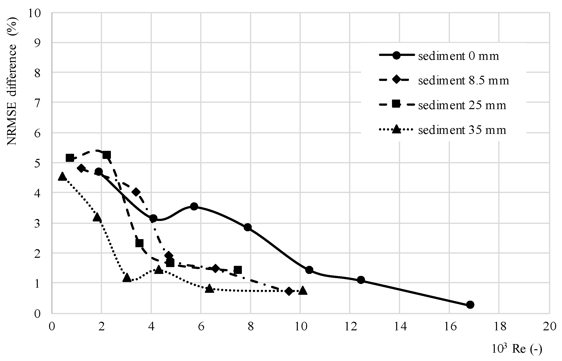
As can be seen in Figure 4, the Gaussian approximation function (Figure 4a) is more precise in a higher range of the velocities and Reynolds number (within the range of our experiments), whereas the Gumbel as well as the GEV approximation (Figure 4b,c) are more precise in lower range of velocities and Reynolds number. It should be noted that the GEV approximation was in all cases more precise than the Gaussian approximation function. This is due to the fact that the GEV approximation is a three-parametric function which is more adaptable to different hydraulic conditions, including the occurrence of dead zones. The difference between the normalised root mean square error (NRMSE) of both approaches is shown in Figure 12.
As can be seen in this figure, the difference between the NRMSE is significant in the lower range of the Reynolds number from 0 up to 6000 (12,000 eventually, in the case of no sediment); in the higher range of Reynolds numbers the difference between both approaches is less than 1%. Based on this comparison, we recommend the use of the Gaussian approximation function (Equation (3)) within the range of Reynolds number Re > 12,000.
6. Conclusions
This paper describes and presents results of experiments focused on pollution transport and dispersion in conditions of flow with low water depth and velocity in sewers with bottom sediment and deposits. Such conditions occur very often in separate sewer systems or in combined systems during dry weather periods.
This study answers three questions which were asked during our research. The first question was how the sediments influence the flow and dispersion processes in the above-described hydraulic conditions. The results of this study showed and confirmed that the value of the coefficient Dx for the case of circular sewer pipe with sediment and deposits decreases almost linearly to a certain limit (inflexion point), which is individual for each particular sediment thickness. Below this limit, the value of the dispersion coefficient rises again. The inflexion point in our experiments occurred at velocities ranged from 0.2 to 0.3 m·s−1, in the Reynold number range from 4000 up to 6000. From the results it can be assumed that at higher layers of sediments the inflexion point occurs at a lower value of Re. This means that the dispersion process depends on the sediment layer thickness and also on the character of the sediment top layer. In real sewer environments, the character of the sediment top layer is subject to temporary changes, e.g., the sediment could be washed out during the rain events in combined sewer system; in contrast, in dry weather the sediment layer is built up as the top layer is formed. This could be a future research objective, as well as the comparison of the laboratory experiment results with results in real sewer networks.
The second objective relates to the presence of temporary transitional (dead) zones and their impact on dispersion processes. The abovementioned flow disintegration and forming of flow with different depths make conditions for dead zones forming and occurrence. Analysing the experimental results, it can be stated that the ratio (and in this way the impact) of dead zones increases with decreasing flow rate and increasing sediment thickness in a pipe. The cause for this is that the water depth decrease causes the change of ratio between areas of active zone and dead zones, and thus the decreasing ratio between the active and passive (dead) zones starts to significantly deform the shape of the output concentration distribution in time of the dispersion process.
The final research objective was to assess validity or suitability of the Gaussian approximation function application in conditions of analysed hydraulic experiment, i.e., low flows in sewer pipe with bottom sediment. There we evaluated the accuracy of the Gaussian approximation function and the GEV approximation by using the NRMSE for both approaches. The GEV approximation was in all cases more precise than the Gaussian approximation function. This is due to the fact that the GEV approximation is a three-parametric function, so it is more adaptable to different hydraulic conditions, including the occurrence of dead zones. The difference between both approaches is significant in the lower range of the Reynolds number, thus we recommend the use of the Gaussian approximation function within the range of Reynolds number Re > 12,000. In all other cases (Re < 12,000) a different approach should be used, respecting the influence of transient storage zones.
As a supplement of this study, an approximation equation, which allows the estimation of the value of the dimensionless dispersion coefficient Dx,d, was created. It is a function of the Reynolds number, sediment thickness and pipe diameter. The proposed approximation equation fits very well with the results (NRMSE = 0.37%) and allows us to predict the value of the dimensionless dispersion coefficient Dx,d within the range of the experimental conditions, as described in this paper.
Author Contributions
Study design and concept: M.S. and Y.V., experimental work: M.S. and Y.V., data processing: M.S., paper writing: M.S. and Y.V. All authors have read and agreed to the published version of the manuscript.
Funding
This work was supported by the Scientific Grant Agency VEGA—grant number VEGA 2/0085/20, by the project H2020—“SYSTEM”, grant agreement No. 787128 and by the International R&D cooperation grant MVTS-SYSTEM.
Institutional Review Board Statement
Not applicable.
Informed Consent Statement
Not applicable.
Data Availability Statement
The research data can be found in the [43].
Acknowledgments
The authors also express their thanks for the support to the Warsaw University of Technology, Faculty of Building services, Hydraulics Engineering and Environmental Engineering, namely to Apoloniusz Kodura for providing the hydraulic laboratory for this research and to Fernando Solano from the Faculty of Electronics and Information Technology for his help during this research.
Conflicts of Interest
Both authors declare no real or perceived financial conflict of interests connected with this study.
References
- Banasiak, R. Hydraulic performance of sewer pipes with deposited sediments. Water Sci. Technol. 2008, 57, 1743–1748. [Google Scholar] [CrossRef]
- Taylor, G.I. Dispersion of soluble matter in solvent flowing slowly through a tube. Proc. R. Soc. Lond. Ser. A Math. Phys. Sci. 1953, 219, 186–203. [Google Scholar]
- Taylor, G.I. The dispersion of matter in turbulent flow through a pipe. Proc. R. Soc. Lond. 1954, 223, 446–468. [Google Scholar] [CrossRef]
- Hart, J.R.; Guymer, I.; Sonnenwald, F.; Stovin, V.R. Residence Time Distributions for Turbulent, Critical, and Laminar Pipe Flow. J. Hydraul. Eng. 2016, 142, 04016024. [Google Scholar] [CrossRef]
- Abokifa, A.A.; Xing, L.; Sela, L. Investigating the Impacts of Water Conservation on Water Quality in Distribution Networks Using an Advection-Dispersion Transport Model. Water 2020, 12, 1033. [Google Scholar] [CrossRef] [Green Version]
- Romero-Gomez, P.; Choi, C.Y. Axial Dispersion Coefficients in Laminar Flows of Water-Distribution Systems. J. Hydraul. Eng. 2011, 137, 1500–1508. [Google Scholar] [CrossRef]
- Rieckermann, J.; Neumann, M.B.; Ort, C.; Huisman, J.; Gujer, W. Dispersion coefficients of sewers from tracer experiments. Water Sci. Technol. 2005, 52, 123–133. [Google Scholar] [CrossRef]
- Hart, J.; Sonnenwald, F.; Stovin, V.; Guymer, I. Longitudinal Dispersion in Unsteady Pipe Flows. J. Hydraul. Eng. 2021, 147, 04021033. [Google Scholar] [CrossRef]
- Guymer, I.; Dennis, P.; O’Brien, R.; Saiyudthong, C. Diameter and Surcharge Effects on Solute Transport across Surcharged Manholes. J. Hydraul. Eng. 2005, 131, 312–321. [Google Scholar] [CrossRef]
- Mark, O.; Jimoh, M.O. An analytical model for solute mixing in surcharged manholes. Urban Water J. 2016, 14, 443–451. [Google Scholar] [CrossRef]
- Chapra, S.C. Surface Water-Quality Modeling; McGraw-Hill Series in Water Resources and Environmental Engineering; Waveland Press: Long Grove, IL, USA, 1997. [Google Scholar]
- Fischer, H.B.; List, E.J.; Koh, R.C.Y.; Imberger, J.; Brooks, N.H. Mixing in Inland and Coastal Waters; Elsevier BV: Amsterdam, The Netherlands, 1979. [Google Scholar]
- Graf, W.H.; Altinakar, M.S. Fluvial Hydraulics: Flow and Transport Processes in Channels of Simple Geometry; Wiley: Hoboken, NJ, USA, 1998; Volume 42. [Google Scholar]
- Marsalek, J.; Sztruhar, D.; Giulianelli, M.; Urbonas, B. (Eds.) Enhancing Urban Environment by Environmental Upgrading and Restoration; Nato Science Series: IV: Earth and Environmental Sciences; Springer: Berlin/Heidelberg, Germany, 2005; Volume 43. [Google Scholar] [CrossRef]
- Meddah, S.; Saïdane, A.; Hadjel, M.; Hireche, O. Pollutant Dispersion Modeling in Natural Streams Using the Transmission Line Matrix Method. Water 2015, 7, 4932–4950. [Google Scholar] [CrossRef] [Green Version]
- Runkel, R.L.; Broshears, R.E. One-Dimensional Transport with Inflow and Storage (OTIS): A Solute Transport Model for Small Streams; CADSWES—Center for Advanced Decision Support for Water and Environmental Systems, Department of Civil Engineering, University of Colorado: Boulder, CO, USA, 1991. [Google Scholar]
- Halmova, D.; Miklanek, P.; Pekar, J.; Pramuk, B.; Pekarova, P. Longitudinal Dispersion Coefficient in Natural Streams in Slovakia. Bodenkultur 2014, 65, 23–29. [Google Scholar]
- Singh, S.K.; Beck, M.B. Dispersion Coefficient of Streams from Tracer Experiment Data. J. Environ. Eng. 2003, 129, 539–546. [Google Scholar] [CrossRef]
- Julínek, T.; Riha, J. Longitudinal dispersion in an open channel determined from a tracer study. Environ. Earth Sci. 2017, 76, 592. [Google Scholar] [CrossRef]
- Socolofsky, S.A.; Gerhard, H.J. Special Topics in Mixing and Transport Processes in the Environment. In Coastal and Ocean Engineering Division, 5th ed.; Texas A&M University: College Station, TX, USA, 2005; p. 171. [Google Scholar]
- Martin, J.L.; McCutcheon, S.C. Hydrodynamics and Transport for Water Quality Modeling; CRC Press: Boca Raton, FL, USA, 2018. [Google Scholar] [CrossRef]
- Rutherford, J.C. River Mixing; Wiley: Hoboken, NJ, USA, 1994. [Google Scholar]
- Gualtieri, C. Numerical Simulation of Flow Patterns and Mass Exchange Processes in Dead Zones. In Proceedings of the IEMSs 4th Biennial Meeting—Int. Congress on Environmental Modelling and Software: Integrating Sciences and Information Technology for Environmental Assessment and Decision Making, Universitat Politècnica de Catalunya, Barcelona, Catalonia, Spain, 7–10 July 2008; Volume 1, pp. 150–161. Available online: https://www.iemss.org/wp-content/iemss2008/uploads/Main/Vol1-iEMSs2008-Proceedings.pdf (accessed on 3 September 2021).
- De Smedt, F.; Brevis, W.; Debels, P. Analytical solution for solute transport resulting from instantaneous injection in streams with transient storage. J. Hydrol. 2005, 315, 25–39. [Google Scholar] [CrossRef]
- De Smedt, F. Analytical solution and analysis of solute transport in rivers affected by diffusive transfer in the hyporheic zone. J. Hydrol. 2007, 339, 29–38. [Google Scholar] [CrossRef]
- Deng, Z.-Q.; Jung, H.-S.; Ghimire, B. Effect of channel size on solute residence time distributions in rivers. Adv. Water Resour. 2010, 33, 1118–1127. [Google Scholar] [CrossRef]
- Shucksmith, J.D.; Boxall, J.B.; Guymer, I. Effects of emergent and submerged natural vegetation on longitudinal mixing in open channel flow. Water Resour. Res. 2010, 46, W04504. [Google Scholar] [CrossRef]
- Shucksmith, J.; Boxall, J.B.; Guymer, I. Determining longitudinal dispersion coefficients for submerged vegetated flow. Water Resour. Res. 2011, 47, W10516. [Google Scholar] [CrossRef]
- Murphy, E.; Ghisalberti, M.; Nepf, H. Model and laboratory study of dispersion in flows with submerged vegetation. Water Resour. Res. 2007, 43, W05438. [Google Scholar] [CrossRef]
- Davis, P.M.; Atkinson, T.C. Longitudinal dispersion in natural channels: An aggregated dead zone model applied to the River Severn, U.K. Hydrol. Earth Syst. Sci. 2000, 4, 373–381. [Google Scholar] [CrossRef]
- Czernuszenko, W.; Rowinski, P.; Sukhodolov, A. Experimental and numerical validation of the dead-zone model for longitudinal dispersion in rivers. J. Hydraul. Res. 1998, 36, 269–280. [Google Scholar] [CrossRef]
- Sokáč, M.; Velísková, Y.; Gualtieri, C. Application of Asymmetrical Statistical Distributions for 1D Simulation of Solute Transport in Streams. Water 2019, 11, 2145. [Google Scholar] [CrossRef] [Green Version]
- Li, G.; Abrahams, A.D.; Atkinson, J.F. Correction factors in the determination of mean velocity of overland flow. Earth Surf. Process. Landf. 1996, 21, 509–515. [Google Scholar] [CrossRef]
- Elder, J.W. The dispersion of marked fluid in turbulent shear flow. J. Fluid Mech. 1959, 5, 544–560. [Google Scholar] [CrossRef]
- Rapp, B. Microfluidics: Modelling, Mechanics and Mathematics; Elsevier BV: Amsterdam, The Netherlands, 2017. [Google Scholar]
- Jobson, H.E.; Froehlich, D.C. Basic Hydraulic Principles of Open-Channel Flow; US Geological Survey: Fairbanks, AK, USA, 1988.
- Ng, H.C.-H.; Cregan, H.L.F.; Dodds, J.M.; Poole, R.J.; Dennis, D.J.C. Partially filled pipes: Experiments in laminar and turbulent flow. J. Fluid Mech. 2018, 848, 467–507. [Google Scholar] [CrossRef] [Green Version]
- Manina, M.; Halaj, P. Sensitivity Analysis of Input Data in Surface Water Quality Models. Acta Hortic. Regiotect. 2019, 22, 84–87. [Google Scholar] [CrossRef] [Green Version]
- Manina, M.; Halaj, P.; Jurík, L.; Kaletová, T. Modelling seasonal changes of longitudinal dispersion in the Okna river. Acta Sci. Pol. Form. Circumiectus 2020, 19, 37–46. [Google Scholar] [CrossRef]
- Stránský, D.; Kabelkova, I.; Bares, V.; Stastna, G.; Suchorab, Z. Suitability of combined sewers for the installation of heat exchangers. Ecol. Chem. Eng. S 2016, 23, 87–98. [Google Scholar] [CrossRef] [Green Version]
- Dulovičová, R. Transformation of bed silts along lowland channel Gabčíkovo-Topoľníky and comparison of their saturated hydraulic conductivity values. Acta Hydrol. Slovaca 2019, 20, 151–159. [Google Scholar] [CrossRef]
- Danckwerts, P. Continuous flow systems: Distribution of residence times. Chem. Eng. Sci. 1953, 2, 1–13. [Google Scholar] [CrossRef]
- Sokáč, M.; Velísková, Y. Longitudinal Dispersion in Sewer Pipes with Sediments. Mendeley Data V1 2021. [Google Scholar] [CrossRef]
Figure 1.
Scheme of the experimental device.

Figure 2.
Example of (a) a dataset and (b) the detail of one experiment concentration distribution in time (Tp—peak time, Tc—centroid time, RFUB—Raw Fluorescence Units Blanked).
Figure 2.
Example of (a) a dataset and (b) the detail of one experiment concentration distribution in time (Tp—peak time, Tc—centroid time, RFUB—Raw Fluorescence Units Blanked).

Figure 3.
Example of a raw and averaged (approximated) data (experiment Nr. 2.4).

Figure 4.
Normalised root mean square error (NRMSE) for (a) the Gaussian approximation function according to Equation (3), (b) the Gumbel approximation function according to Equation (4) and (c) the GEV approximation according to Equation (5).
Figure 4.
Normalised root mean square error (NRMSE) for (a) the Gaussian approximation function according to Equation (3), (b) the Gumbel approximation function according to Equation (4) and (c) the GEV approximation according to Equation (5).

Figure 5.
Relationship between Dx and uc from tracer experiments results. Dx is evaluated according to Gaussian approximation function (Equation (3)).
Figure 5.
Relationship between Dx and uc from tracer experiments results. Dx is evaluated according to Gaussian approximation function (Equation (3)).

Figure 6.
Relationship between Dx and Re from tracer experiments results. Dx is evaluated according to Gaussian approximation function (Equation (3)).
Figure 6.
Relationship between Dx and Re from tracer experiments results. Dx is evaluated according to Gaussian approximation function (Equation (3)).

Figure 7.
Relationship between Dx,d and Re from tracer experiments results. Dx is evaluated according to Gaussian approximation function (Equation (3)).
Figure 7.
Relationship between Dx,d and Re from tracer experiments results. Dx is evaluated according to Gaussian approximation function (Equation (3)).

Figure 8.
Results of tracer experiments—normalised cumulative residence time distribution (CRTD). The particular image tagging (a–d) corresponds with the experiment groups in Table 2.
Figure 8.
Results of tracer experiments—normalised cumulative residence time distribution (CRTD). The particular image tagging (a–d) corresponds with the experiment groups in Table 2.

Figure 9.
Results of tracer experiments—normalised concentration distributions in time. The particular image tagging (a–d) corresponds with the experiment groups in Table 2.
Figure 9.
Results of tracer experiments—normalised concentration distributions in time. The particular image tagging (a–d) corresponds with the experiment groups in Table 2.

Figure 10.
Results of tracer experiments—mass normalised concentration distributions in time, time is without normalisation. The particular image tagging (a–d) corresponds with the experiment groups in Table 2.
Figure 10.
Results of tracer experiments—mass normalised concentration distributions in time, time is without normalisation. The particular image tagging (a–d) corresponds with the experiment groups in Table 2.

Figure 11.
Results of the Dx,d–Gaussian approximation function according to Equation (11), H/D is the sediment/pipe diameter ratio.
Figure 11.
Results of the Dx,d–Gaussian approximation function according to Equation (11), H/D is the sediment/pipe diameter ratio.

Figure 12.
Difference of the normalised root mean square error (NRMSE) between the Gaussian approximation function according to Equation (3) and the GEV approximation according to Equation (5).
Figure 12.
Difference of the normalised root mean square error (NRMSE) between the Gaussian approximation function according to Equation (3) and the GEV approximation according to Equation (5).


Table 1.
Summary of the tracer experiments results.
| Sediment | Exp. Nr. | Discharge | Water Depth | uc | up | Dx | Dx,G | Dx,GEV | ξ | Re | Pe | Dx,d | NRMSE | ||
|---|---|---|---|---|---|---|---|---|---|---|---|---|---|---|---|
| Gauss | Gumbel | GEV | |||||||||||||
| (-) | (L·s−1) | (mm) | (m·s−1) | (m·s−1) | (m2·s−1) | (m2·s−1) | (m·s−1) | (-) | (-) | (-) | (-) | % | % | % | |
| 0 mm | 0.1 | 0.145 | 10.4 | 0.197 | 0.211 | 0.0110 | 0.0158 | 0.016 | 0.020 | 1933 | 0.12 | 11.81 | 5.44 | 0.83 | 0.77 |
| 0.2 | 0.422 | 15.5 | 0.282 | 0.293 | 0.0078 | 0.0131 | 0.013 | −0.038 | 4120 | 0.36 | 4.68 | 4.46 | 1.55 | 1.33 | |
| 0.3 | 0.505 | 19.6 | 0.312 | 0.324 | 0.0082 | 0.0138 | 0.014 | −0.027 | 5761 | 0.48 | 3.54 | 4.87 | 1.54 | 1.36 | |
| 0.4 | 0.839 | 24.0 | 0.349 | 0.361 | 0.0081 | 0.0137 | 0.014 | −0.080 | 7907 | 0.66 | 2.61 | 3.98 | 1.82 | 1.16 | |
| 0.5 | 1.170 | 29.6 | 0.372 | 0.385 | 0.0098 | 0.0167 | 0.017 | −0.153 | 10,382 | 0.70 | 2.50 | 3.29 | 3.40 | 1.87 | |
| 0.6 | 1.628 | 34.4 | 0.384 | 0.397 | 0.0105 | 0.0178 | 0.019 | −0.167 | 12,454 | 0.79 | 2.26 | 3.78 | 4.24 | 2.71 | |
| 0.7 | 2.237 | 40.3 | 0.444 | 0.458 | 0.0137 | 0.0235 | 0.025 | −0.238 | 16,881 | 0.81 | 2.31 | 3.40 | 5.59 | 3.17 | |
| 8.5 mm | 1.1 | 0.147 | 7.7 | 0.168 | 0.181 | 0.0149 | 0.0262 | 0.026 | −0.005 | 1217 | 0.08 | 23.23 | 6.01 | 1.23 | 1.22 |
| 1.2 | 0.410 | 16.6 | 0.216 | 0.232 | 0.0098 | 0.0164 | 0.016 | 0.003 | 3399 | 0.28 | 5.98 | 4.97 | 0.98 | 0.96 | |
| 1.3 | 0.589 | 20.6 | 0.244 | 0.270 | 0.0081 | 0.0138 | 0.014 | 0.024 | 4733 | 0.45 | 3.82 | 3.98 | 2.15 | 2.10 | |
| 1.4 | 0.799 | 24.7 | 0.284 | 0.306 | 0.0078 | 0.0134 | 0.013 | −0.024 | 6615 | 0.61 | 2.82 | 3.87 | 2.55 | 2.42 | |
| 1.5 | 1.114 | 30.7 | 0.330 | 0.343 | 0.0078 | 0.0134 | 0.014 | −0.118 | 9542 | 0.82 | 2.14 | 3.10 | 3.13 | 2.39 | |
| 25 mm | 2.1 | 0.140 | 5.9 | 0.139 | 0.157 | 0.0221 | 0.0380 | 0.038 | −0.004 | 775 | 0.03 | 49.88 | 6.70 | 1.58 | 1.57 |
| 2.2 | 0.392 | 14.3 | 0.166 | 0.181 | 0.0130 | 0.0216 | 0.022 | 0.090 | 2241 | 0.15 | 10.84 | 7.06 | 2.39 | 1.85 | |
| 2.3 | 0.600 | 18.1 | 0.210 | 0.220 | 0.0078 | 0.0134 | 0.014 | −0.107 | 3586 | 0.39 | 4.43 | 3.68 | 2.38 | 1.40 | |
| 2.4 | 0.794 | 20.2 | 0.252 | 0.260 | 0.0069 | 0.0118 | 0.012 | −0.158 | 4800 | 0.58 | 3.04 | 2.98 | 3.29 | 1.33 | |
| 2.5 | 1.227 | 24.6 | 0.324 | 0.330 | 0.0073 | 0.0126 | 0.013 | −0.188 | 7519 | 0.82 | 2.18 | 2.84 | 4.04 | 1.44 | |
| 35 mm | 3.1 | 0.141 | 8.4 | 0.059 | 0.084 | 0.0431 | 0.0686 | 0.077 | 0.318 | 467 | 0.01 | 173.08 | 8.34 | 5.02 | 3.79 |
| 3.2 | 0.410 | 14.2 | 0.138 | 0.155 | 0.0149 | 0.0248 | 0.025 | 0.007 | 1847 | 0.11 | 14.61 | 6.96 | 3.92 | 3.76 | |
| 3.3 | 0.633 | 18.2 | 0.178 | 0.188 | 0.0097 | 0.0167 | 0.017 | −0.156 | 3052 | 0.28 | 6.37 | 4.62 | 4.61 | 3.43 | |
| 3.4 | 0.876 | 21.1 | 0.217 | 0.224 | 0.0082 | 0.0141 | 0.015 | −0.163 | 4321 | 0.46 | 3.89 | 3.66 | 4.04 | 2.22 | |
| 3.5 | 1.280 | 25.6 | 0.263 | 0.270 | 0.0087 | 0.0150 | 0.016 | −0.184 | 6352 | 0.61 | 2.96 | 2.91 | 3.97 | 2.10 | |
| 3.6 | 2.070 | 30.2 | 0.356 | 0.370 | 0.0119 | 0.0205 | 0.021 | −0.156 | 10,130 | 0.68 | 2.62 | 3.22 | 3.67 | 2.49 | |
Table 2.
Experiment groups.
| Experiment Group | Exp. Nr. | Sediment Thickness | Q | uc | up | Dx | Dx,GEV | ξ | Re | Pe | Dx,d |
|---|---|---|---|---|---|---|---|---|---|---|---|
| (-) | (-) | (mm) | (L·s−1) | (m·s−1) | (m·s−1) | (m2·s−1) | (m2·s−1) | (-) | (-) | (-) | (-) |
| (a) | 0.1 | 0 | 0.145 | 0.197 | 0.211 | 0.011 | 0.0158 | 0.020 | 1933 | 0.12 | 8.20 |
| 1.1 | 8.5 | 0.147 | 0.282 | 0.181 | 0.015 | 0.0262 | −0.005 | 1217 | 0.08 | 13.23 | |
| 2.1 | 25 | 0.140 | 0.312 | 0.157 | 0.022 | 0.0380 | −0.004 | 775 | 0.03 | 29.06 | |
| 3.1 | 35 | 0.141 | 0.349 | 0.084 | 0.043 | 0.0785 | 0.318 | 467 | 0.01 | 102.37 | |
| (b) | 0.2 | 0 | 0.422 | 0.372 | 0.293 | 0.008 | 0.0132 | −0.038 | 4120 | 0.36 | 2.76 |
| 1.2 | 8.5 | 0.410 | 0.384 | 0.232 | 0.010 | 0.0164 | 0.003 | 3399 | 0.28 | 3.58 | |
| 2.2 | 25 | 0.392 | 0.444 | 0.181 | 0.013 | 0.0217 | 0.090 | 2241 | 0.15 | 6.52 | |
| 3.2 | 35 | 0.410 | 0.168 | 0.155 | 0.015 | 0.0248 | 0.007 | 1847 | 0.11 | 8.80 | |
| (c) | 0.3 | 0 | 0.505 | 0.216 | 0.324 | 0.008 | 0.0139 | −0.027 | 5761 | 0.48 | 2.10 |
| 1.3 | 8.5 | 0.589 | 0.244 | 0.270 | 0.008 | 0.0138 | 0.024 | 4733 | 0.45 | 2.25 | |
| 2.3 | 25 | 0.600 | 0.284 | 0.220 | 0.008 | 0.0136 | −0.107 | 3586 | 0.39 | 2.55 | |
| 3.3 | 35 | 0.633 | 0.330 | 0.188 | 0.010 | 0.0172 | −0.156 | 3052 | 0.28 | 3.57 | |
| (d) | 0.4 | 0 | 0.839 | 0.139 | 0.361 | 0.008 | 0.0139 | −0.080 | 7907 | 0.66 | 1.53 |
| 1.4 | 8.5 | 0.799 | 0.166 | 0.306 | 0.008 | 0.0135 | −0.024 | 6615 | 0.61 | 1.64 | |
| 2.4 | 25 | 0.794 | 0.210 | 0.260 | 0.007 | 0.012 | −0.158 | 4800 | 0.58 | 1.72 | |
| 3.4 | 35 | 0.876 | 0.252 | 0.224 | 0.008 | 0.015 | −0.163 | 4321 | 0.46 | 2.19 |
Publisher’s Note: MDPI stays neutral with regard to jurisdictional claims in published maps and institutional affiliations. |
© 2021 by the authors. Licensee MDPI, Basel, Switzerland. This article is an open access article distributed under the terms and conditions of the Creative Commons Attribution (CC BY) license (https://creativecommons.org/licenses/by/4.0/).
Share and Cite
MDPI and ACS Style
Sokáč, M.; Velísková, Y. Impact of Sediment Layer on Longitudinal Dispersion in Sewer Systems. Water 2021, 13, 3168. https://doi.org/10.3390/w13223168
AMA Style
Sokáč M, Velísková Y. Impact of Sediment Layer on Longitudinal Dispersion in Sewer Systems. Water. 2021; 13(22):3168. https://doi.org/10.3390/w13223168
Chicago/Turabian StyleSokáč, Marek, and Yvetta Velísková. 2021. "Impact of Sediment Layer on Longitudinal Dispersion in Sewer Systems" Water 13, no. 22: 3168. https://doi.org/10.3390/w13223168
Note that from the first issue of 2016, this journal uses article numbers instead of page numbers. See further details here.