
Stream Suspended Mud as an Indicator of Post-Mining Landform Stability in Tropical Northern Australia


1
Research Institute for Environment & Livelihoods, Charles Darwin University, Ellengowan Drive, Casuarina, NT 0810, Australia
2
College of Engineering, IT & Environment, Charles Darwin University, Ellengowan Drive, Casuarina, NT 0810, Australia
3
Surface Water & Erosion Solutions, Lakes Crescent, Marrara, NT 0812, Australia
*
Author to whom correspondence should be addressed.
Water 2021, 13(22), 3172; https://doi.org/10.3390/w13223172
Submission received: 20 October 2021
/
Revised: 2 November 2021
/
Accepted: 8 November 2021
/
Published: 10 November 2021
(This article belongs to the Section Water Erosion and Sediment Transport)
Abstract
:Mining can cause environmental disturbances and thus mined lands must be managed properly to avoid detrimental impacts in the future. They should be rehabilitated in such a way that post mining landforms behave similarly as the surrounding stable undisturbed areas. A challenge for government regulators and mine operators is setting closure criteria for assessment of the stability of the elevated post-mining landforms. Stability of a landform is often measured by the number and incision depth of gullies. This can assess mass stability and bulk movement of coarse material. However, there is a need for a more sensitive approach to assess catchment disturbances using the concept of waves of fine suspended sediment and thus determine the dynamics of recovery of a post mining landform. A more environmentally meaningful approach would be to assess the fine suspended sediment (FSS, silt + clay (0.45 µm < diameter < 63 µm)) leaving the system and entering downstream waterways. We propose assessing stability through relationships between rainfall event loads of FSS and event discharge (Q) in receiving streams. This study used an innovative approach where, instead of using instantaneous FSS concentration, it used total FSS load in waves of sediment driven through the system by rainfall runoff events. High resolution stream monitoring data from 2004 to 2015 in Gulungul and Magela Creeks, Northern Territory, Australia, were used to develop a relationship between sediment wave and event discharge, ∑FSS α f(Q). These creeks are adjacent to and receive runoff from Ranger Mine. In 2008, a 10 ha elevated waste rock landform was constructed and instrumented in the Gulungul Creek catchment. The earthworks required to build the landform created a considerable disturbance in the catchment, making a large volume of disturbed soil and substrate material available for erosion. Between 2008 and 2010, in the first two wet seasons immediately after construction, the downstream monitoring site on Gulungul Creek showed elevated FSS wave loads relative to discharge, compared with the upstream site. From 2010 onwards, the FSS loads relative to Q were no longer elevated. This was due to the establishment of vegetation on the site and loose fine sediment being trapped by vegetation. Large scale disturbance associated with mining and rehabilitation of elevated landforms causes elevated FSS loads in receiving streams. The predicted FSS loads for the stream as per the relationships between FSS and event discharge may not show a 1:1 relation with the observed loads for respective gauging stations. When downstream monitoring shows that FSS wave loads relative to rainfall runoff event discharge reduce back to pre-construction catchment levels, it will indicate that the landform is approaching equilibrium. This approach to assess landform stability will increase the sensitivity of assessing post-mining landform recovery and assist rehabilitation engineers to heal the land and benefit owners of the land to whom it is bestowed after rehabilitation.
1. Introduction
The rehabilitation of above-grade landforms that result from mining needs to achieve control of erosion [1] and the ultimate aim is to achieve geomorphic stability. Government regulations and public expectations generally require waste rock landforms to be regraded to neat alignments and grades, but this does not always achieve the main objectives of minimum erosion and long-term stability [2]. It was eloquently stated by Ayres [2] that, “Uniform landforms represent immature topography and are poised to evolve to lower energy states by shallow slope failures or accelerated erosion.” An aim of mine landform stability would be that the elevated landform is in equilibrium with the surrounding topography. However, is equilibrium achievable and how is it to be assessed?
There is a considerable amount of literature discussing geomorphic equilibrium [3]. Equilibrium in relation to landforms, or geomorphic equilibrium, has been described as a constant function between input and output of the overall landform. For example, in a landform at equilibrium, erosion may occur, but over time, the overall input and output of material due to erosion is similar [4]. It does not mean that the landform is static or unchanging, but that it fluctuates as the broader landscape responds to long-term trends. Renwick [4] states as an example that a stream channel will maintain relative cross-section geometry while undergoing long-term degradation under landscape change in the broader scale. Renwick [4] also described two other equilibrium forms—disequilibrium and nonequilibrium. A landform in disequilibrium is one that is not in equilibrium with its surrounds, but is slowly trending toward equilibrium at a rate somewhat similar to a thermodynamic or exponential decay curve. A landform in nonequilibrium does not appear to tend toward equilibrium, but may undergo substantial change as a result of high magnitude/low-frequency events. These events may be weather fluctuations, landslides [5] or other mass failure episodes [4].
Mining operations cause significant environmental disturbance, and if not managed appropriately may have detrimental impacts. Rehabilitation of disturbed sites is the process of returning the land to an acceptable state. It varies depending on the agreed values of end land use, and it typically occurs in multiple stages, which can take many years to complete [6]. Creating a post-mining elevated landform that is in equilibrium with the surrounding catchment is a significant challenge.
Mine closure criteria often require a stable landform where rates of erosion do not exceed that of the surrounding undisturbed catchment and downstream sediment loads do not exceed pre-mining sediment loads. However, assessing the stability of a landform is a significant challenge. It is often the case that sediment loads have not been measured pre-mining and decisions must be made based on upstream measurements post-mining. A waste rock dump (WRD) during the mining process is a nonequilibrium landform. Prior to revegetation and engineered amelioration, the landform is in nonequilibrium even after reshaping. Nonequilibrium landforms can undergo sudden and substantial outputs caused by low-frequency/high-magnitude events such as landslides and large rainfall events [4]. Through rehabilitation processes such as revegetation and engineered drainage lines, erosion control and sediment-traps, the aim is that a WRD becomes a disequilibrium landform that will trend toward equilibrium. Once an elevated mine landform moves from nonequilibrium to disequilibrium trending toward equilibrium it needs to be confirmed so that regulatory authorities can confidently sign-off on rehabilitation and closure criteria. However, the landform could also revert from equilibrium to disequilibrium as a result of climate change or human impact.
Ranger mine in Northern Territory (12°41′ S, 132°55′ E), Australia has been producing uranium oxide (U3O8) since 1981 and is presently undergoing rehabilitation and closure. The mine site is surrounded by, but separate from, the World Heritage listed Kakadu National Park. Elevated WRD landforms and the tailings dam are being reshaped based on landform evolution modelling (LEM) using the Siberia LEM and the CAESAR-Lisflood LEM. Mining ceased in 2012 with milling of the mined ore continuing to early 2021 and work is now focused on rehabilitation [6]. Initial modelling focused on using SIBERIA and CAESAR LEMs to determine whether the uranium remaining in the waste rock would remain buried for 10,000 years. Landform evolution modelling (LEM) methods were developed through a significant amount of research including: field programs using plot and catchment studies to calibrate sediment transport and hydrology models for the calibration of the Siberia LEM and assessing mine landform stability over a 1000 y period [7,8,9,10]; using catchment denudation rates, empirical modelling and numerical modelling to assess the Ranger landform design [10]; field studies to assess the temporal change in Siberia parameter values as a landscape matures [11]; assessing the impact of extreme rainfall events in the Ranger landform using CEASAR-Lisflood [9]; simulating long-term (up to 10,000 y) erosion, on the Ranger landform, the effects of climate change [12,13,14,15,16]; comparison of the undisturbed Magela Creek catchment and the mine-disturbed catchment using CAESAR-Lisflood simulations [17]; and large scale trial landform studies [18,19]. Although the landform design is not yet final, simulations using CAESAR-Lisflood [9,15] indicate that the final landform prior to revegetation and engineering will be in geomorphic nonequilibrium and that periodic high intensity events will result in high erosion events and export of sediment to the receiving streams. The challenge is how to assess when the landform reaches a state of disequilibrium that is trending toward equilibrium with the surrounding country post-mine closure. Then, closure criteria can be agreed on and signed-off by stakeholders, i.e., the traditional owners, government and community groups.
To assess equilibrium relationships, increased mud or fine suspended sediment (FSS; silt + clay, <63µm, >0.45µm) concentrations and loads in receiving streams may be a useful indicator of catchment disturbance. The Ranger mine is adjacent to Magela Creek [6] and Gulungul Creek is a small tributary of Magela Creek. Gulungul Creek is one of the tributaries that would be the first to receive sediment generated from the mine site during and after rehabilitation [20]. Gulungul and Magela Creeks are ephemeral sand-bed anabranching streams which carry sand loads (bed and suspended bed) and small FSS loads. Detailed stream mud monitoring over a period of 22 years at Magela Creek and Gulungul Creek in the Magela Creek catchment [21,22,23,24,25,26,27,28] has been conducted to assess mining impact on receiving streams downstream of the Ranger mine. Increased mud (FSS; silt + clay, <63 µm, >0.45 µm) concentrations and loads in streams after a catchment disturbance such as fires, cyclones, excavations, construction, mining and extreme rainfall events is a phenomenon often observed [29,30,31,32,33,34] and quantified. FSS is highly mobile and many contaminants that may have been released by the disturbance attach themselves to FSS. Therefore, a knowledge of FSS transport is important in assessing contaminant transport [35]. It has also been observed that after the disturbance scar has healed itself, downstream FSS concentration/loads return to pre-disturbance levels [29,30,31,34,36].
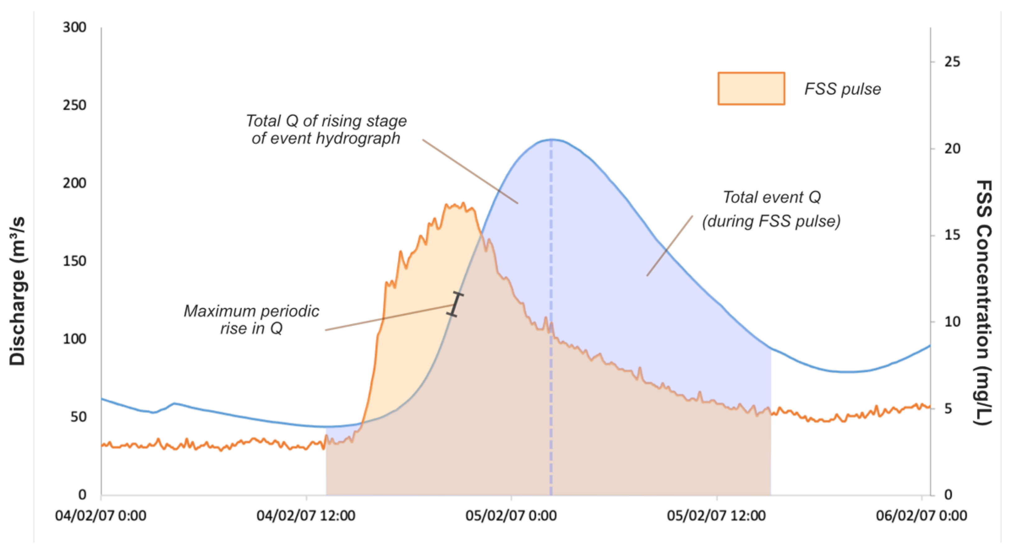
In order to estimate a catchment disturbance by the indication of increased FSS in the receiving streams, it is necessary to calculate the background levels of FSS in a non-disturbed state of the landform. Instantaneous FSS is difficult to sample, but there is a strong correlation between turbidity (NTU) and mud concentration (the silt and clay component of suspended sediment). Thus, continuous NTU data could be used to monitor stream concentration (mud C) within the catchment [37]. The relationships between instantaneous FSS concentration (C) and instantaneous discharge (Q) are very difficult to fit because of the large scatter that exists because the hysteresis between C and Q [30,38] and recently numerous studies have been conducted assessing different methods of estimating stream suspended sediment loads based on discharge (e.g., [39]). However, a relationship between FSS and Q is necessary to assess impacts due to disturbances. Evans et al. [7], Evans et al. [30], and Moliere and Evans [11] assessed event-based relationships using data from erosion studies on Ranger mine and natural catchments at Tin Camp Creek. Evans et al. [30] identified pulses or waves of sediment moving through a stream associated with hydrograph flood waves and derived a relationship between total FSS load in a wave and the cumulative discharge in the rising stage of the flood wave of the form:
where Q is instantaneous discharge (m3 s−1), Qp is peak event discharge, Q0 is initial discharge, and m and K are fitted parameters. The rising stage discharge to Qp is used, as this is the most easily defined period of flow for a number of events and it is this part of the hydrograph that carries most of the FSS (Figure 1).
Using this relationship Evans et al. [30] observed a system change where for the first year after a disturbance, the relationship between total FSS load and the rising stage of the flood wave changed (Figure 2). Once the disturbance scar had healed the relationship returned to baseline, i.e., pre-disturbance conditions. Following this, Moliere et al. (2004) fitted relationships between total event wave FSS load and rising stage total Q. Using this relationship, predicted total FSS load was compared to observed total FSS load and as expected the relationship found to be 1:1. In a later study by Moliere and Evans [36], relationships were fitted to Magela Creek and Gulungul Creek and it was found that after a disturbance, using equations for total FSS load derived from monitoring data, the relationship was no longer 1:1, but the observed load was higher than the equation-predicted load. The same was not observed at upstream sites where the predicted–observed relationship remained at 1:1.
This method was proposed to assess if the post-closure landform was returning to “equilibrium” with its surrounds. However, based on the LEM studies done on Ranger mine, it is more appropriate to assess if the landform was in disequilibrium changing to equilibrium. Earlier studies show that during construction of the landform, surface material is disturbed, and large volumes of sediment will be made available for transport. Therefore, it is expected that immediately after closure, FSS concentration/loads will be elevated and observed loads will be higher than predicted using the derived equation. This means that the best fit line for the relationship post-disturbance will move in an upward direction and as the disturbance equilibrated, the best fit line moves downwards to the undisturbed state (Figure 2). This was confirmed by Moliere and Evans [36] who fitted relationships for 6 sites and amended Equation (1) as follows:
where T = total event FSS mass (kg), QT = total event discharge (m3), Ri = Δqt (m3 s−1) (change in instantaneous rising discharge during measured time interval), and k (kg m−3 FSS−3), a, and b are fitted parameters. It is proposed that Equation (2) is useful to determine the FSS load driven through the system by the rising hydrograph thereby avoiding the complexities of the hysteresis.
Moliere and Evans [36] confirmed that if a change in the best fit occurs downstream and not upstream, this indicates that it is caused by a disturbance between the sites. If it occurs upstream and downstream, it indicates a disturbance upstream of the upstream site or a catchment-wide unusual event. They also changed the method of assessment. Instead of using the relationship between FFS event load and total event discharge (Figure 2) [38], they used a relationship between the observed total event FFS load (OTL) and predicted total event FSS load (PTL) using Equation (2). In the undisturbed state the best fit line between OTL and PTL is the 1:1 line. If the relationship for the downstream site moves away from the 1:1 line, but stays the same at the upstream site, then, an event introducing greater FSS total loads at the downstream site has occurred between the upstream and downstream sites. It is evident that this methodology can be used to determine catchment disturbance. However, its application in understanding the dynamics of landform stability followed by a series of anthropological activities such as mining and consequent rehabilitation is yet to be assessed.
Development of a framework to assess how a landform will return to its pre-disturbance sediment flows after mining and rehabilitation is desired. At the Ranger mine this was done by studying the sensitivity of a landform to disturbance and the effect of subsequent rehabilitation efforts such as revegetation. Moliere and Evans [36] assessed FSS and NTU from 2004 to 2008 at four locations to calculate OTL and the equations for PTL. The four locations were monitoring sites in Gulungul Creek downstream (GCDS), Gulungul Creek upstream (GCUS), Magela Creek down-stream (MCDS), and Magela Creek Upstream (MCUS) of the mine. During the 2008 Dry Season, a 50 ha trial landform was constructed on the Ranger site within the Gulungul Creek catchment. The trial landform is on the right bank of Gulungul Creek between Gulungul Creek upstream and Gulungul Creek downstream and is several hundred metres from the creek draining through savanna woodland and heavily vegetated black soil swamps near the stream channel. The only significant disturbance in the catchment is the Ranger mine. FSS, NTU, rainfall and discharge data were collected at all monitoring sites from 2004 to 2015 enabling how a landform will return to its pre-disturbance sediment flows after mining and rehabilitation to be assessed.
Stability of a landform is often measured by the number and incision depth of gullies which can assess mass stability and bulk movement of coarse material. However, there is a need for a more sensitive approach to assess catchment disturbances using the concept of waves of fine suspended sediment and thus determine the dynamics of recovery of a post mining landform. This approach to assess landform stability will increase the sensitivity of assessing post-mining landform recovery and assist rehabilitation engineers to heal the land and benefit owners of the land to whom it is bestowed after rehabilitation. The aims of this study included updating the equations between FSS and NTU at all four locations to calculate the observed total event FSS load (OTL) and the equations for predicted total (PTL), incorporating new data from the rehabilitation phase. The methodology described in the paragraphs above was then used to assess the catchment disturbance in the succeeding years after trial landform construction to determine the response to rehabilitation. This assessment can throw light on how the whole Ranger mine site landform will behave after rehabilitation and closure.
2. Materials and Methods
2.1. Study Area and Monitoring Site Data
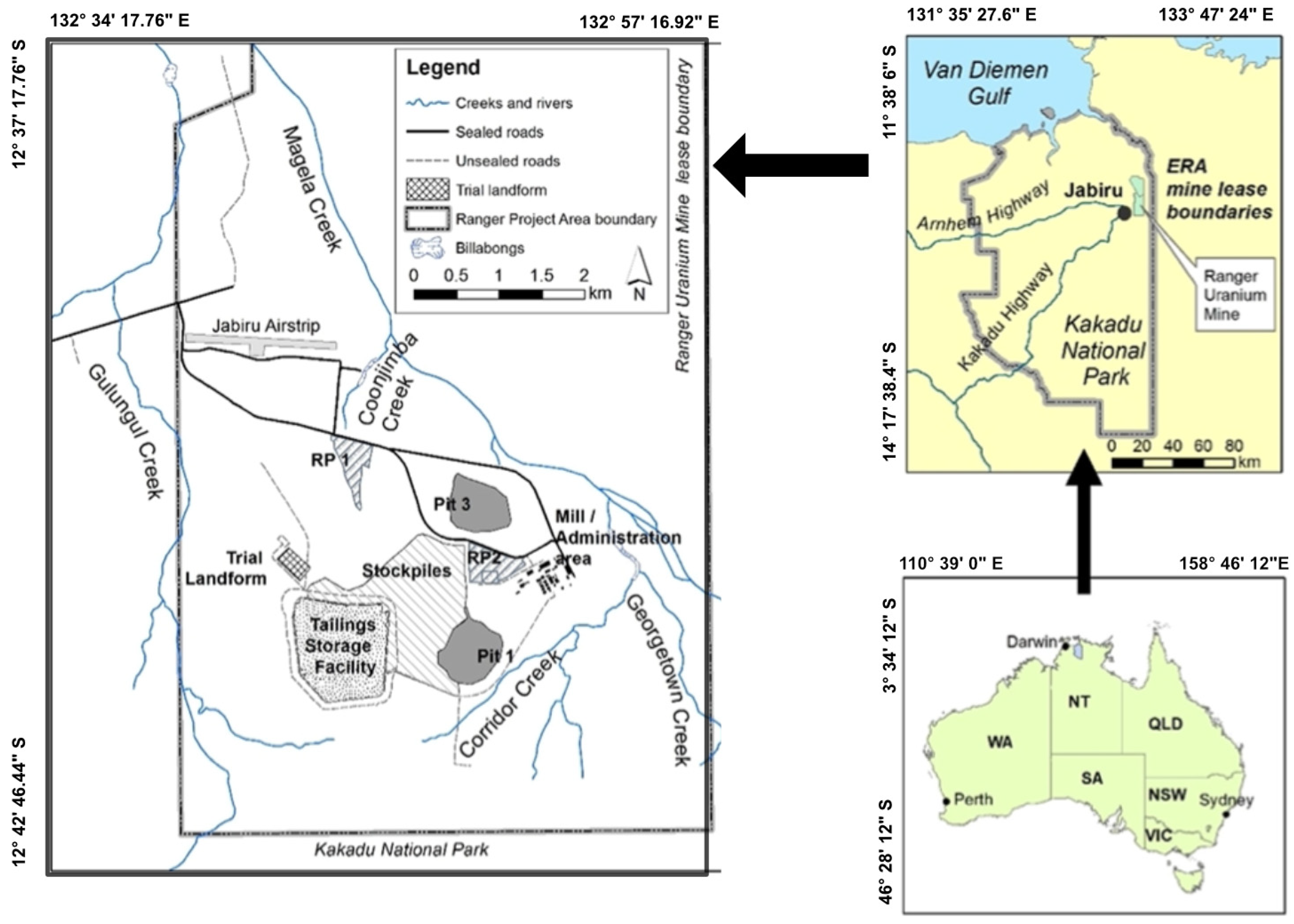
Ranger mine (12°41′ S, 132°55′ E) is an open cut uranium mine operated by Energy Resources of Australia Ltd. (ERA) and is in the Alligator Rivers Region of the Northern Territory, Australia. The mine is located 8 km east of the township of Jabiru and within the 78 km2 Ranger Project Area which is surrounded by, but separate from, the World Heritage listed Kakadu National Park (Figure 3). The Ranger mine is adjacent to Magela Creek, a tributary of the East Alligator River [6]. Gulungul Creek is a small tributary of Magela Creek that is adjacent to the tailing dam. It is one of the tributaries that would be the first to receive sediment generated from the mine site during and after rehabilitation [20]. Gulungul and Magela Creeks are ephemeral sand-bed braided streams which carry very large sand loads (bed and suspended bed) and small FSS loads.
Environmental Research Institute of the Supervising Scientist (eriss) has monitoring sites in Gulungul Creek downstream (GCDS), Gulungul Creek upstream (GCUS), Magela Creek downstream (MCDS), and Magela Creek upstream (MCUS) of the mine (Figure 4). The data provided by eriss were continuous discharge (m3) and turbidity (NTU) and FSS (<63 µm fraction of sediment samples collected in the auto-samplers; mg). Data were from August 2004 to August 2015 measured at a frequency of 6 min for Gulungul Creek and 10 min for Magela Creek at GCDS, GCUS, MCDS, and MCUS. Storm events (Figure 1) for analysis were extracted from the continuous data for analysis as described in Section 2.3. Laboratory analyses data were also provided to enable assessment of NTU/FSS concentration relationships.
2.2. Assessment of Existing Relationships between NTU and FSS
FSS data could not be collected for each rainfall event, but NTU data can be used as a surrogate for FSS [37]. The NTU–FSSNTU–FSS relationships at each site in Gulungul and Magela Creeks can be used to accurately estimate FSS and create a continuous FSS record. The relationship can vary between sites and with different instruments and it is important that the FSS data be collected regularly to update and confirm the FSS–NTUFSS–NTU relationship. The FSS–NTU relationship was plotted with available data for each gauging station and the equation of the best fit line was calculated using the trendline function in Excel. Trendlines were calculated using the exponential and linear options and the trendline with the highest R value was used to determine the FSS–NTU relationship. Hence, the FSS concentration was determined using the equation from the trendline and the continuous NTU data collected.
2.3. Selection of Rainfall–Runoff Events for Analysis
In order to calculate the event FSS load and event discharge characteristics, it is necessary to segregate a rainfall runoff event from the annual stream discharge data by analyzing the rise and fall of FSS concentration in the stream pertaining to a rainfall event. Discharge and FSS data were plotted on the y-axis and the timeline on x-axis (as shown in Figure 1) for each water year (31st August to 31st August) from 2005 to 2015. An FSS concentration of 2–5 mg/L was considered as the base flow level. Each event resulting in an FSS pulse where the sedigraph rises and reaches a peak concentration >5 mg/L was identified. The start of the FSS pulse was taken as a point where the sedigraph started to rise with a steep slope up to a peak value. The end of the FSS pulse was taken as a point on the sedigraph where the slope of the receding part of sedigraph was first parallel with the x-axis [36]. Here, the event FSS loads and event discharge for corresponding rainfall-runoff events are thus determined by adding instantaneous discharge and FSS loads corresponding to the time intervals from the start to end of an identified rainfall–runoff event. It is also same as the shaded area under the graph shown in Figure 1 for event discharge and event FSS loads, respectively.
2.4. Updating Relationships Describing the Variation of Rainfall–Runoff Event FSS Mass with Total Event Discharge
The relationship between event FSS load and the runoff characteristics total event discharge (QT) and maximum periodic rise in discharge (Ri) were determined using a multivariate regression analysis. The runoff characteristics total event runoff (QT) and maximum periodic rise in discharge (Ri) were chosen as they are the most significant runoff characteristics for predicting event FSS load within the region [36]. Total FSS load, QT, and Ri were calculated for each rainfall-runoff event identified in Section 2.3. A total of 110 events were analysed for Gulungul Creek upstream, 100 events for Gulungul Creek downstream, and 60 events for Magela Creek downstream. The results of these analyses were used to update Equation (2) in Moliere and Evans [36]. The values for the parameters in Equation (2) for each event were calculated based on the new data and the equation for total event load for each of the sites was determined. The event data analysed for Gulungul and Magela are presented in Appendix A.
2.5. Comparison of PTL and OTL for Each Event Data Analyzed to Determine Catchment Disturbance and Assessing the Effect of Trial Landform on FSS in Gulungul Creek and Magela Creek
For each event data analyzed, OTL was calculated using the FSS–NTU relationship and PTL was calculated for updated Equation (2) for each site. The OTL versus PTL graph for Magela and Gulungul was produced for each year from 2004 to 2015 to assess the effect of the trial landform construction and rehabilitation on FSS event loads in Gulungul Creek and Magela Creek.
3. Results and Discussion
The first step was to determine the FSS–NTU relationship to predict continuous FSS load. Then, the continuous FSS load data were used to derive the equations for the relationship between FSS load and discharge events from 2005 to 2015. The relationship between predicted and observed FSS load at each of the monitoring locations was then assessed over time to evaluate the responses of the catchments in the succeeding years after trial landform construction.
3.1. FSS–NTU Relationship
To assess the relationship between FSS and discharge events during the period from 2005 to 2015, first, it was necessary to derive continuous FSS data using the relationship between FSS and NTU. The relationships between FSS and NTU were updated as these relationships can vary between instruments, sites and over time. The FSS–NTU relationships for GCUS, GCDS, MCUS, and MCDS derived with the available data are presented below.
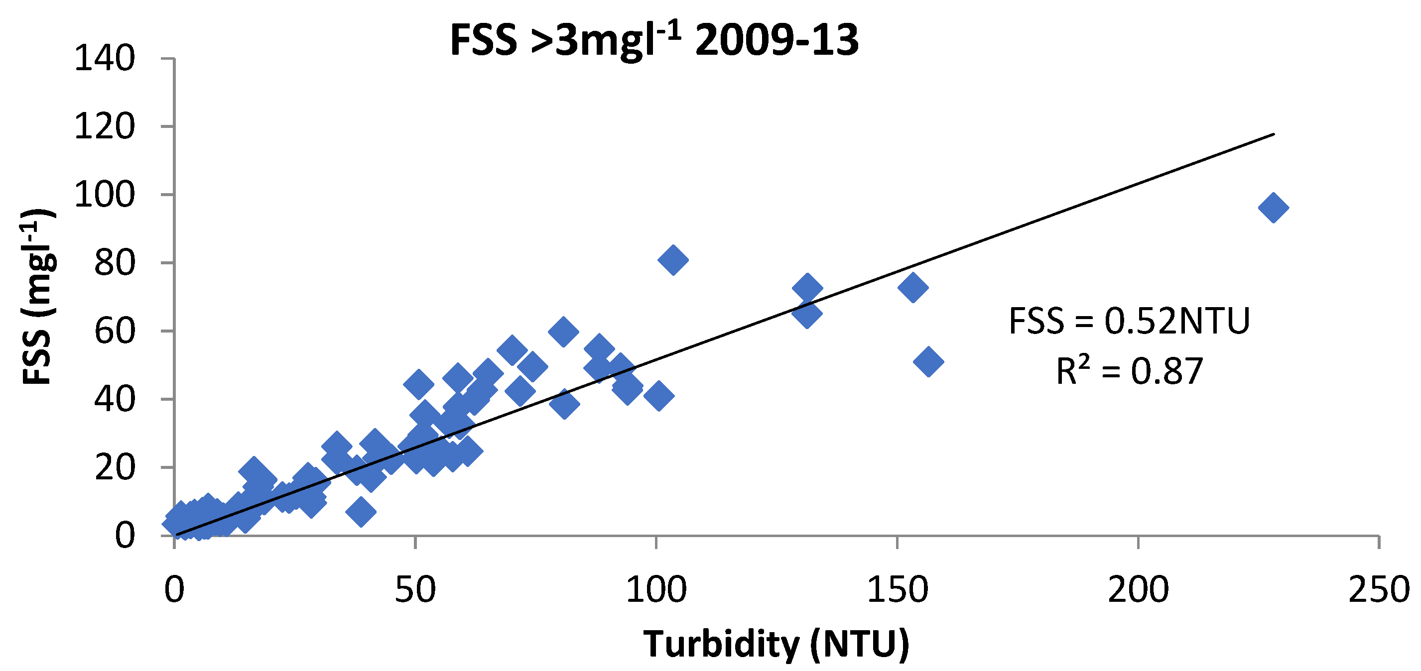
For GCUS, the NTU/FSS relationship determined from data for 2009–2013 is shown in Figure 5 and Equation (3) 2009 to 2013:
The relationship between FSS and NTU at GCUS derived by Moliere et al. [41] using the data available at that time (discontinuous data between 2004 to 2007) was:
Because, Equation (3) had a higher R2 value than Equation (4), the earlier will be used for analysis of GCUS events.
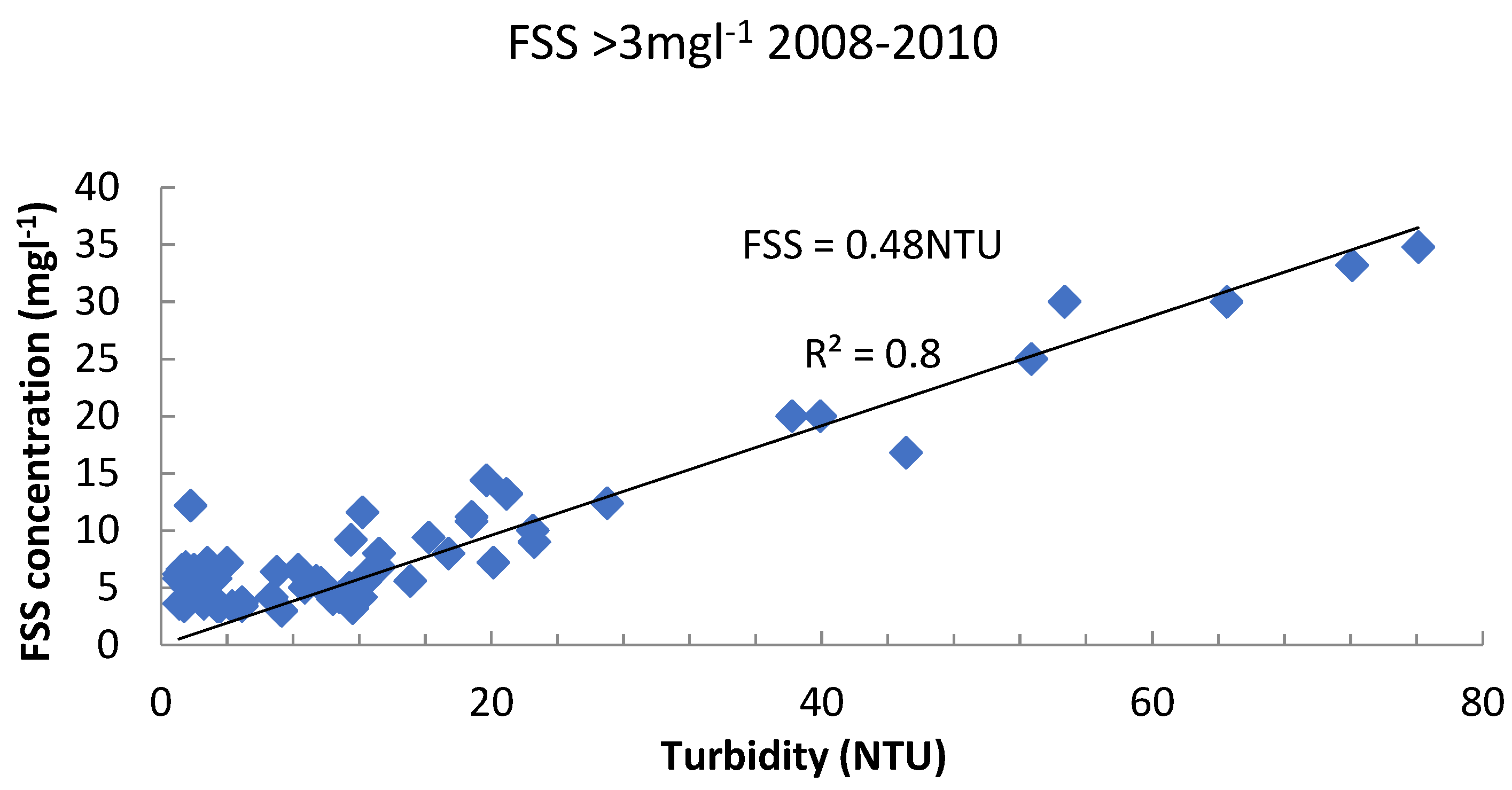
For GCDS, the NTU–FSS relationship determined for data from 2008–2010 is shown in Figure 6.
The relationship at GCDS derived by Moliere et al. [41] using data between 2005 and 2007 is:
Because the relationship derived by Moliere et al. [41] in Equation (5) had a higher R2 value than determined for the data in Figure 6, the relationship derived by Moliere et al. [41] was used for deriving FSS for analysis.
No new FSS data were available for MCUS and MCDS. Therefore, the relationship between NTU and FSS derived by Moliere et al. [36] using the data between 2006 and 2008 was used to derive FSS for all the Magela Creek data.
The relationships between FSS and NTU were found to accurately estimate FSS and therefore a continuous FSS record was created from the observed NTU data. The OTL for FSS pulse events for each station were calculated from these equations.
3.2. FSS-QT Relationship
The FSS-QT relationship was derived as per the methodology described in Section 2.4 and the equations for Magela and Gulungul are as follows:
The PTL for FSS pulse events for each station were determined from these equations.
3.3. Assessing Catchment Disturbance Due to Trial Landform on FSS in Gulungul Creek and Magela Creek
3.3.1. Trial Landform Disturbance
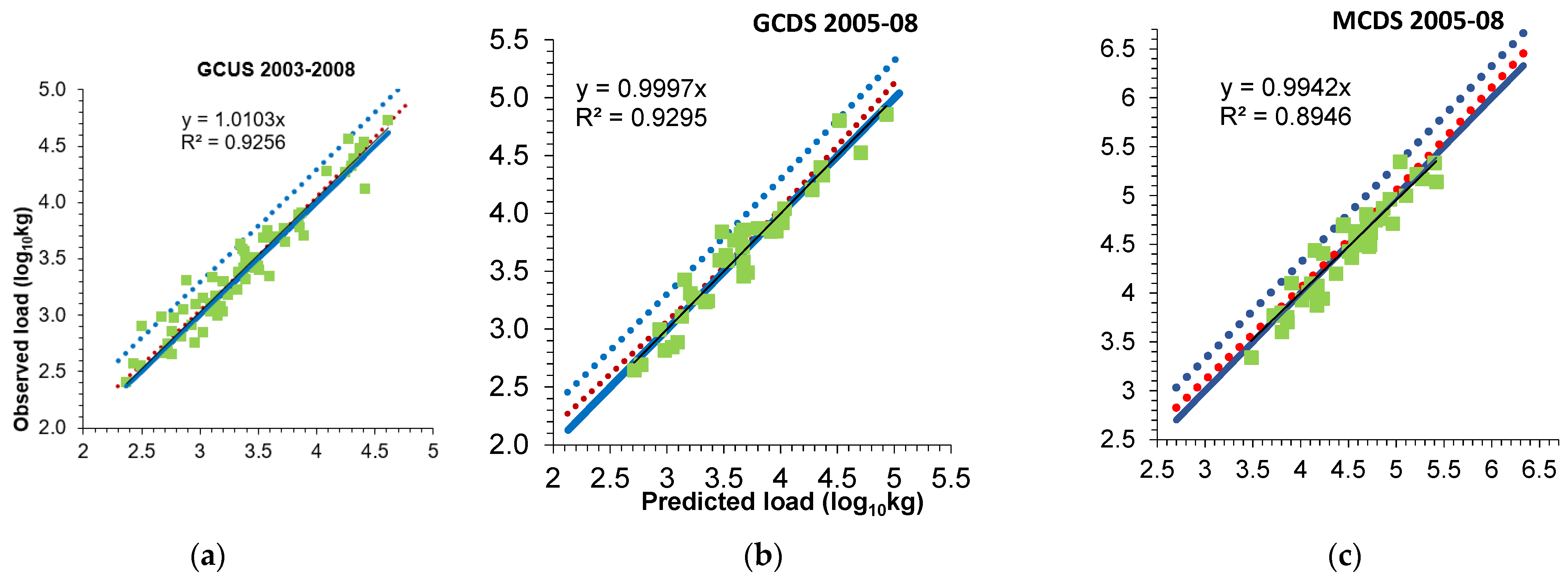
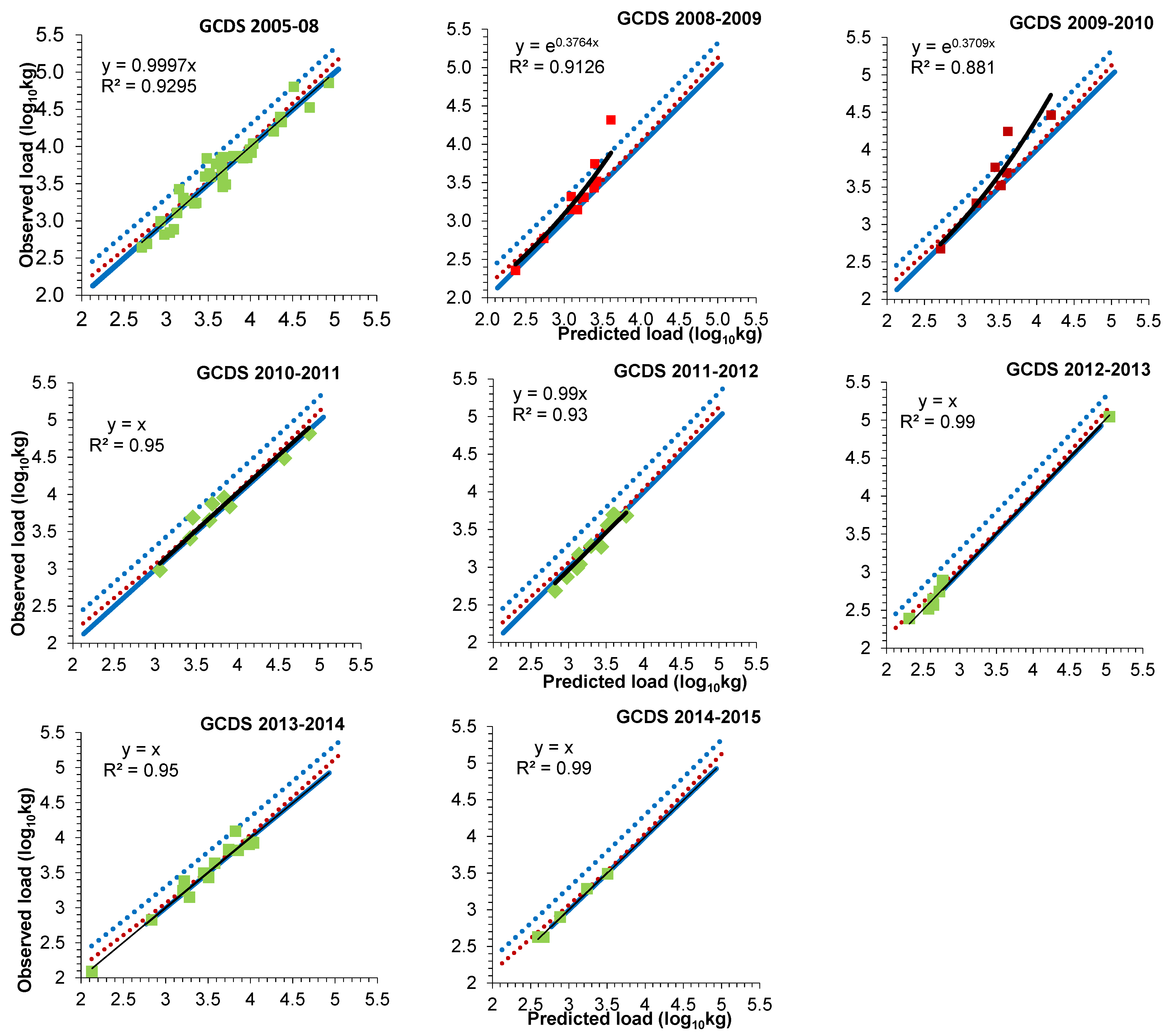
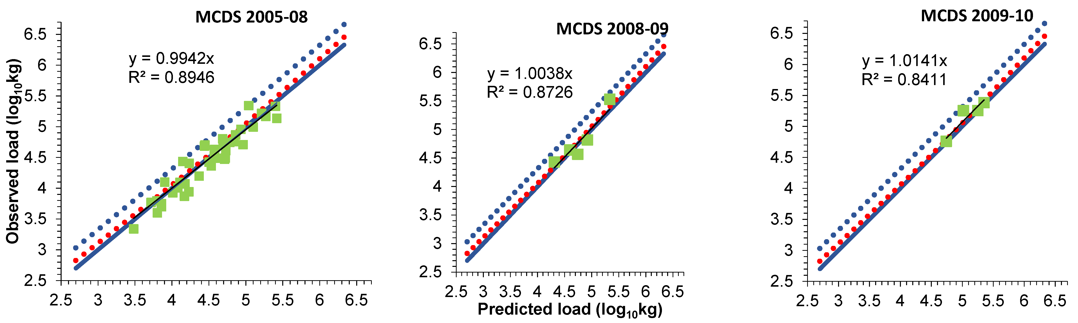
Events for water years from 2004 to 2015 were analysed to assess the impacts of the trial landform constructed in 2008, with respect to elevated FSS event mass. In Figure 7, Figure 8, Figure 9 and Figure 10, the relationship between predicted event log10 FSS load for GCUS, GCDS, and MCDS (Equations (7), (8) and (10)) and observed event log10 FSS load (Equations (4)–(6)) are shown. Individual event data for Gulungul and Magela Creeks are shown in Appendix A.
This analysis supports the theory that a system change in FSS mass can be observed downstream as a result of catchment disturbance, in this case trial landform construction, and that this system change will return to baseline as the disturbance “heals itself”. For the years till 2008 (Figure 7), prior to the construction of trial landform and the potential impact on Gulungul Creek, the original fitted line using the events analysed is in congruence with the 1:1 line. This relationship represents the functioning of the catchment system with respect to total FSS mass transported during rainfall runoff events for GCUS, GCDS, and MCDS (Figure 7a,b,c, respectively). The only likely source of disturbance in the catchment is the Ranger mine as there has been very little disturbance elsewhere in the catchment.
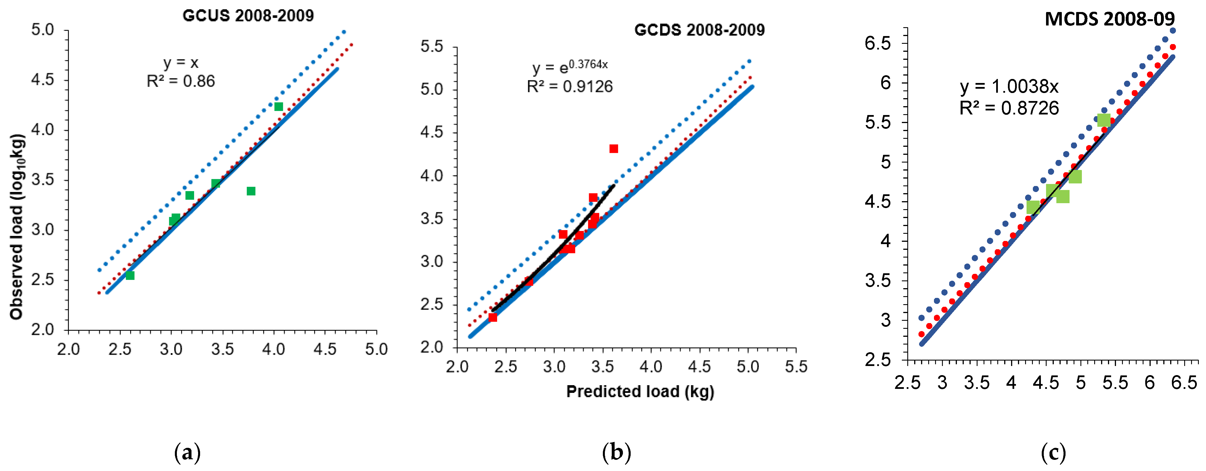
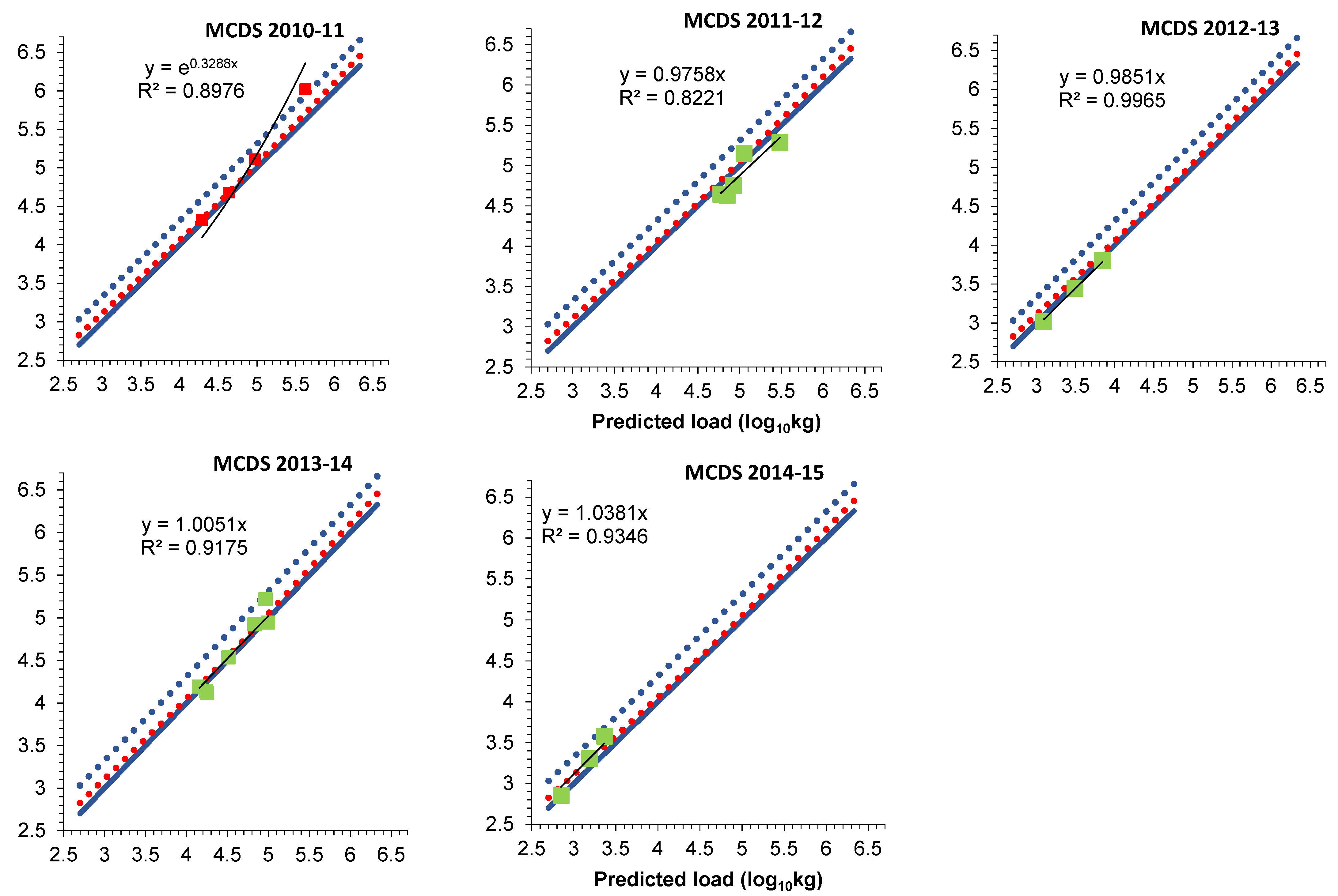
Immediately after construction of the trial landform, there was a system change in GCDS in 2008–2009 (Figure 8) and 2009–2010 (Figure 9), but not in GCUS and MCDS. At GCDS, the total FSS mass has increased relative to total event discharge as shown by the black fitted line in Figure 8b and Figure 9b. The best fit line for these years in GCDS is an exponential function with large events falling on or above the 95% prediction limit of the 2005–2008 1:1 line. The exponential nature of the best fit indicates that as event size increases so does the event total FSS mass relative to that which is predicted. The larger events have the greatest excursions above the 95% prediction limit. At the same time, the fitted line for events in GCUS and MCDS is linear, and within the confidence limits of the original fitted line. Thus, they showed no disturbance and the lack of broader disturbance across the catchment confirmed that it was the trial landform construction in Gulungul catchment that caused the system change. One of the large events that had FSS loads much greater than the predicted value, which depicted system change at GCDS, was the event on 17 February 2009. The morning after this event, sediment-laden water was observed flowing from the trial landform towards GCDS at Ranger mine site (Saynor pers. Obs.).
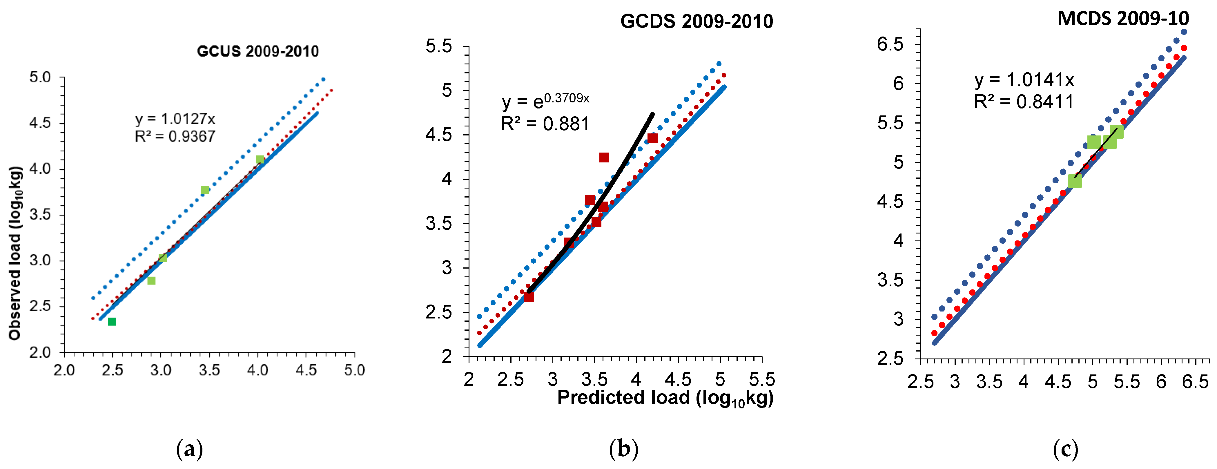
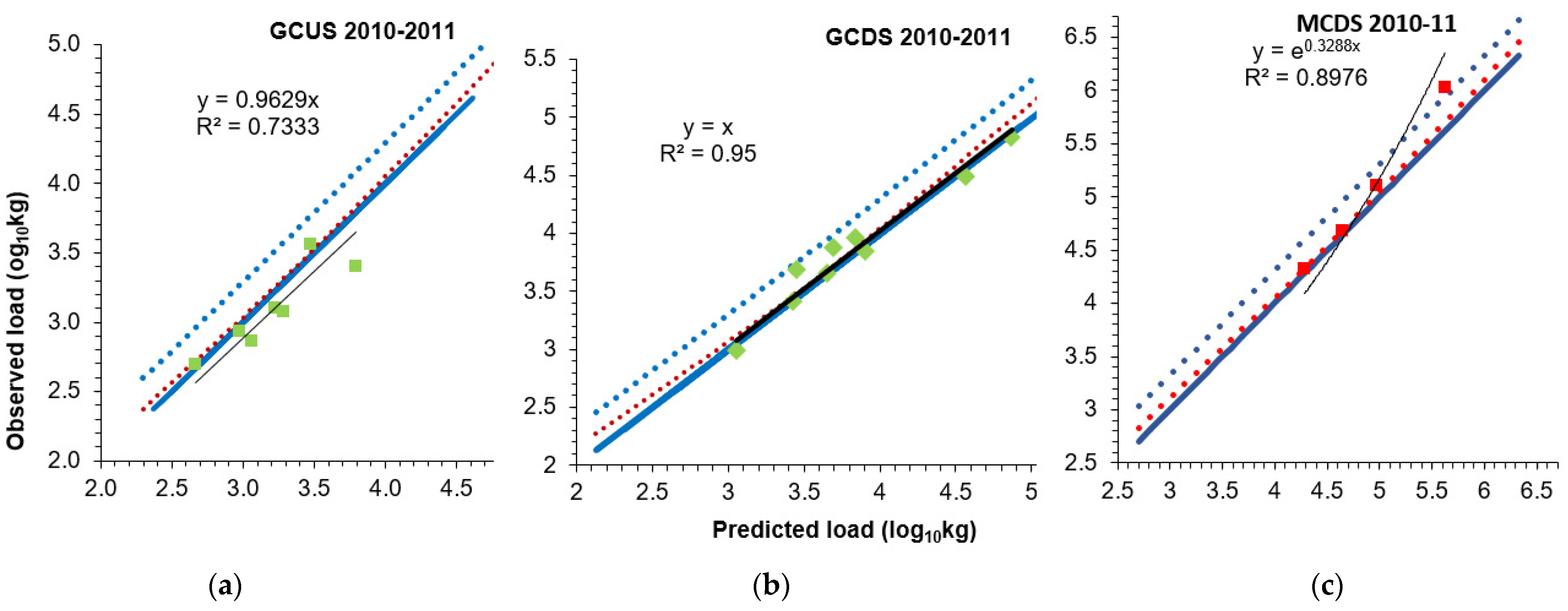
During the following years there was recovery in the catchment. This is shown by the reduction in total FSS load relative to event discharge with the fitted line moving downward toward the blue line in GCDS (Figure 10b). This corresponded to some settling of the trial landform. By 2010-11 the catchment was functioning at pre-trial landform conditions, as even very large FSS load events fell on the 1:1 line. The best fit lines for these later years were again linear rather than exponential (Appendix B).
Studies show that vegetation can reduce erosion over time [42]. Simulations by Saynor et al. [19] showed that ripping the surface of the trial landform and without vegetation created a landform in disequilibrium that moved toward equilibrium with pulses of sediment about every 10 years that reduced with time. Simulations of a ripped surface with vegetation showed a landform that commenced in disequilibrium, but became in equilibrium in about 3 years. Our study corroborates that paper, as the trial landform showed catchment recovery after 2 to 3 years. This may be attributed to vegetation on the trial landform in addition to the natural stabilisation of the land over time.
3.3.2. Magela Creek Downstream—2010–2011
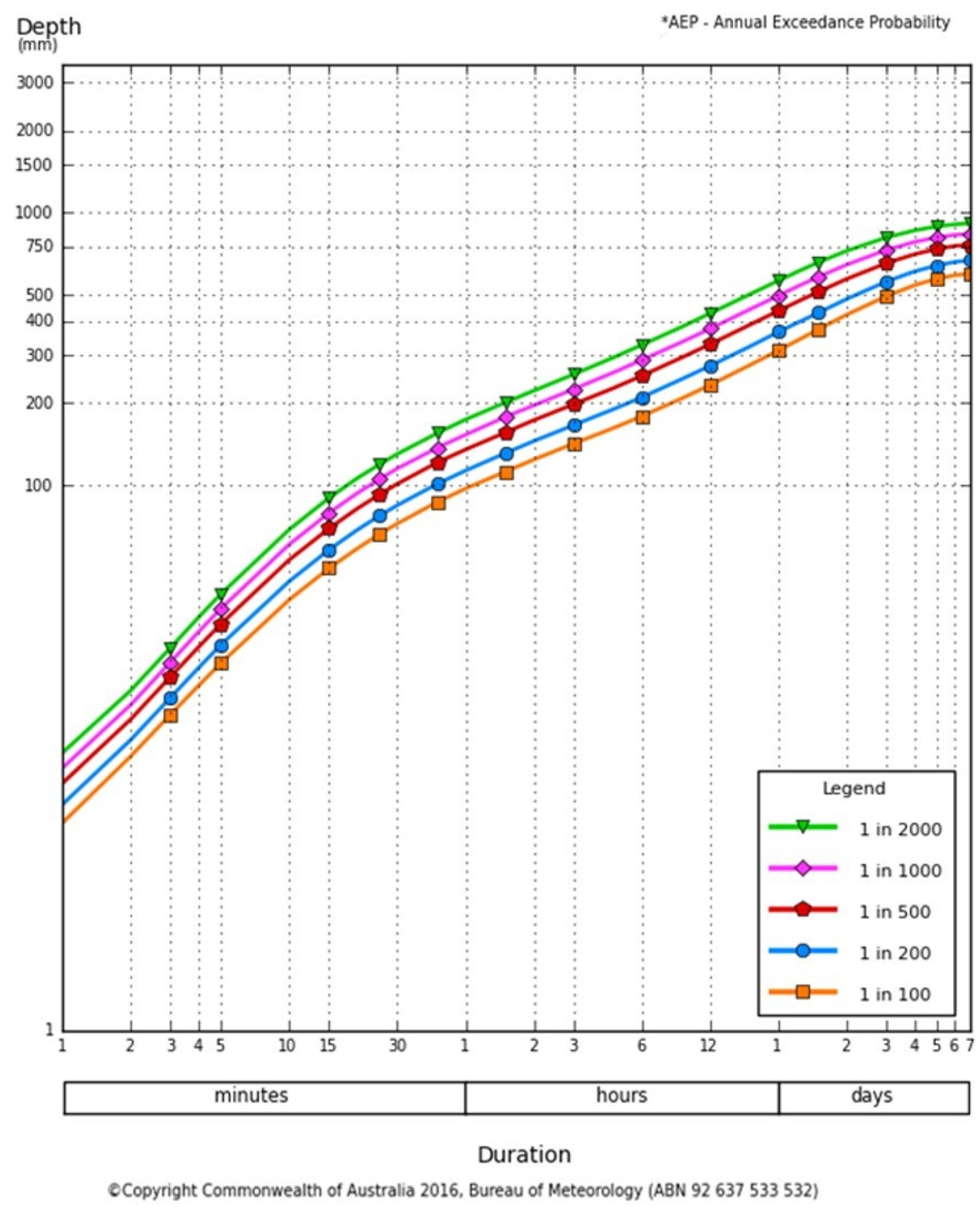
In February 2011, tropical Cyclone Carlos formed over Darwin, 217 km from Jabiru and on 22nd of February 2011, a thunderstorm at Jabiru resulted in a total of 190 mm of rain in a day, including 70.2 mm in 34 min (≈1% AEP—annual exceedance probability) and 119.8 mm in 94 min [43] (≈0.5–0.2% AEP) (Figure 11). The daily rainfall recorded at Magela downstream gauging station (G821009) on 22nd February 2011 was 103.5 mm [44]. The event on 22nd February lies above the 95% prediction limit of the 1:1 best fit line in Figure 10c. Such an extraordinary rainfall event triggered a system change (Figure 10c). How the extreme rainfall event interacted with disturbance in the catchment and caused the elevated FSS loads to rise above the predicted background levels is unknown.
4. Conclusions
In conclusion, the methodology described in the paper can be used to assess catchment disturbance and landform stability. In this study, the return to equilibrium following catchment disturbance at Ranger mine was able to be determined by measuring the FSS load spikes and relating them to the expected relationship between event discharge and event FSS loads in the receiving streams. FSS spikes above the background relationship, in the creeks with catchments where the mine resides acted as an indicator of the catchment disturbance. The methodology successfully identified the catchment where the disturbance occurred. Field verification is necessary to identify whether the disturbance source is mine related.
This method is sensitive and can be applied as a mine landform rehabilitation assessment tool. During landform disturbance, there will be FSS spikes in receiving waters. Then, as the rehabilitated site approaches equilibrium with the surrounding catchment, the FSS spikes should return to pre-mining levels. Once this is achieved, a landform may be considered stable. Therefore, monitoring of NTU, discharge, and regular FSS concentration to confirm the FSS–NTU relationship can be used to assess post mining land-form stability. Beneficiaries from this research include government regulators, mining environmental staff, and in case of Ranger mine, the traditional owners of the land. Future prospects for the research would be to automatically determine the boundaries of FSS discharge event spikes to enable development of an application for environmental officials to easily input values and parameters of the landform to assess stability.
Author Contributions
Conceptualization: K.G.E. and D.N.; methodology: K.G.E. and D.N.; formal analysis: K.G.E., D.N. and M.R.N.; writing—original draft preparation: D.N. and K.G.E.; writing—review and editing: D.N., K.G.E. and S.B.; project administration: K.G.E. All authors have read and agreed to the published version of the manuscript.
Funding
Not applicable.
Institutional Review Board Statement
Not applicable.
Informed Consent Statement
Not applicable.
Acknowledgments
The Environmental Research Institute of the Supervising Scientist (eriss) is thanked for the provision of the data for this study. Professor Ken Evans’s time was provided by Surface & Erosion Solutions as an in-kind contribution.
Conflicts of Interest
The authors declare no conflict of interest.
Appendix A

Table A1.
GCDS event data analysed.
| Event No. | Date | Event Mud Load(kg) | Event Discharge (Q) (m3) | Peak Rising Discharge Rate (Ri-6) (m3s−1) |
|---|---|---|---|---|
| 1 | 18-Jan-06 | 5137 | 890,108 | 0.29 |
| 2 | 21-Jan-06 | 8277 | 1,911,959 | 0.50 |
| 3 | 28-Jan-06 | 1859 | 358,956 | 0.09 |
| 4 | 09-Feb-06 | 3911 | 661,240 | 0.29 |
| 5 | 12-Feb-06 | 2034 | 326,757 | 0.14 |
| 6 | 18-Feb-06 | 4349 | 630,721 | 0.35 |
| 7 | 22-Feb-06 | 7452 | 1,174,759 | 0.53 |
| 8 | 22-Feb-06 | 1714 | 432,803 | 0.22 |
| 9 | 31-Mar-06 | 1283 | 278,227 | 0.13 |
| 10 | 02-Apr-06 | 6971 | 1,539,699 | 0.44 |
| 11 | 04-Apr-06 | 16,011 | 3,102,354 | 4.34 |
| 12 | 21-Jan-07 | 990 | 184,275 | 0.07 |
| 13 | 10-Feb-07 | 6612 | 862,991 | 0.29 |
| 14 | 27-Feb-07 | 33,459 | 7,974,887 | 6.40 |
| 15 | 28-Feb-07 | 71,685 | 13,401,584 | 5.70 |
| 16 | 09-Mar-07 | 9088 | 1,685,654 | 2.45 |
| 17 | 19-Mar-07 | 5856 | 753,932 | 0.34 |
| 18 | 20-Mar-07 | 7199 | 906,272 | 0.33 |
| 19 | 24-Mar-07 | 7008 | 1,629,238 | 1.09 |
| 20 | 29-Mar-07 | 491 | 127,240 | 0.08 |
| 21 | 31-Mar-07 | 1748 | 457,943 | 0.17 |
| 22 | 04-Jan-08 | 3936 | 586,172 | 0.15 |
| 23 | 04-Jan-08 | 63,502 | 5,283,436 | 4.92 |
| 24 | 06-Jan-08 | 6922 | 591,338 | 0.30 |
| 25 | 13-Jan-08 | 697 | 233,728 | 0.09 |
| 26 | 29-Jan-08 | 441 | 114,063 | 0.05 |
| 27 | 04-Feb-08 | 2667 | 310,704 | 0.04 |
| 28 | 14-Feb-08 | 2862 | 953,718 | 0.12 |
| 29 | 15-Feb-08 | 21,336 | 3,818,541 | 4.86 |
| 30 | 18-Feb-08 | 3081 | 1,005,092 | 0.20 |
| 31 | 29-Feb-08 | 10,954 | 1,981,688 | 0.58 |
| 32 | 01-Mar-08 | 25,050 | 3,785,046 | 2.47 |
| 33 | 04-Mar-08 | 7419 | 1,405,497 | 0.84 |
| 34 | 16-Mar-08 | 770 | 266,513 | 0.06 |
| 35 | 16-Mar-08 | 3827 | 925,945 | 0.20 |
| 36 | 23-Mar-08 | 654 | 207,150 | 0.05 |
| 37 | 29-Dec-08 | 229 | 51,576 | 0.06 |
| 38 | 22-Jan-09 | 595 | 114,528 | 0.12 |
| 39 | 17-Feb-09 | 20,836 | 741,880 | 0.95 |
| 40 | 23-Feb-09 | 5602 | 503,495 | 0.17 |
| 41 | 26-Feb-09 | 2051 | 372,146 | 0.12 |
| 42 | 27-Feb-09 | 2089 | 263,180 | 0.07 |
| 43 | 12-Mar-09 | 1419 | 263,180 | 0.09 |
| 44 | 13-Mar-09 | 2735 | 467,923 | 0.47 |
| 45 | 15-Mar-09 | 3296 | 503,283 | 0.47 |
| 46 | 16-Mar-09 | 1413 | 310,437 | 0.10 |
| 47 | 07-Jan-10 | 474 | 111,861 | 0.08 |
| 48 | 14-Jan-10 | 3330 | 679,641 | 0.10 |
| 49 | 23-Jan-10 | 17,642 | 787,705 | 0.34 |
| 50 | 27-Jan-10 | 5835 | 547,900 | 0.23 |
| 51 | 29-Jan-10 | 1936 | 322,418 | 0.12 |
| 52 | 01-Feb-10 | 29,042 | 2,741,737 | 1.02 |
| 53 | 12-Apr-10 | 4933 | 762,585 | 0.33 |
| 54 | 11-Jan-11 | 7471 | 978,363 | 0.18 |
| 55 | 12-Jan-11 | 2575 | 553,120 | 0.09 |
| 56 | 15-Jan-11 | 9014 | 1,296,616 | 0.45 |
| 57 | 21-Jan-11 | 4482 | 926,514 | 0.11 |
| 58 | 24-Jan-11 | 4875 | 569,141 | 0.20 |
| 59 | 31-Jan-11 | 966 | 239,773 | 0.10 |
| 60 | 13-Feb-11 | 30,657 | 5,998,246 | 4.00 |
| 61 | 22-Feb-11 | 66,222 | 10,828,969 | 23.25 |
| 62 | 25-Feb-11 | 6911 | 1,455,769 | 0.85 |
| 63 | 18-Dec-11 | 1933 | 426,689 | 0.05 |
| 64 | 21-Dec-11 | 4939 | 774,143 | 0.41 |
| 65 | 26-Dec-11 | 4811 | 1,041,777 | 1.25 |
| 66 | 31-Jan-12 | 3593 | 649,114 | 0.24 |
| 67 | 07-Feb-12 | 1878 | 512,732 | 0.51 |
| 68 | 08-Feb-12 | 4971 | 763,572 | 0.25 |
| 69 | 18-Feb-12 | 1103 | 290,340 | 0.14 |
| 70 | 03-Mar-12 | 747 | 198,615 | 0.10 |
| 71 | 28-Mar-12 | 492 | 137,253 | 0.16 |
| 72 | 21-Apr-12 | 979 | 267,151 | 0.12 |
| 73 | 09-May-12 | 1477 | 285,181 | 0.11 |
| 74 | 23-Dec-12 | 246 | 38,881 | 1.41 |
| 75 | 28-Jan-13 | 558 | 114,627 | 0.07 |
| 76 | 28-Jan-13 | 780 | 120,929 | 0.18 |
| 77 | 11-Feb-13 | 331 | 83,144 | 0.06 |
| 78 | 19-Feb-13 | 439 | 95,555 | 0.05 |
| 79 | 07-Mar-13 | 372 | 93,669 | 0.10 |
| 80 | 15-Mar-13 | 110,886 | 17,462,579 | 4.87 |
| 81 | 29-Mar-13 | 669 | 148,523 | 0.07 |
| 82 | 06-Dec-13 | 123 | 30,825 | 0.04 |
| 83 | 29-Dec-13 | 6554 | 1,395,337 | 0.25 |
| 84 | 16-Jan-14 | 8585 | 1,858,834 | 1.10 |
| 85 | 18-Jan-14 | 1408 | 367,808 | 0.45 |
| 86 | 23-Jan-14 | 4304 | 725,409 | 0.40 |
| 87 | 24-Jan-14 | 12,326 | 1,202,057 | 1.12 |
| 88 | 27-Jan-14 | 2708 | 637,085 | 0.22 |
| 89 | 30-Jan-14 | 2400 | 338,803 | 0.16 |
| 90 | 11-Feb-14 | 6703 | 1,030,467 | 0.61 |
| 91 | 12-Feb-14 | 3101 | 536,734 | 0.48 |
| 92 | 13-Feb-14 | 8403 | 1,907,867 | 1.60 |
| 93 | 17-Feb-14 | 8026 | 1,674,141 | 2.14 |
| 94 | 18-Feb-14 | 2026 | 333,243 | 0.22 |
| 95 | 12-Mar-14 | 1747 | 327,679 | 0.15 |
| 96 | 10-Jan-15 | 421 | 104,403 | 0.05 |
| 97 | 25-Jan-15 | 792 | 169,699 | 0.05 |
| 98 | 29-Jan-15 | 1925 | 363,245 | 0.09 |
| 99 | 24-Feb-15 | 3086 | 631,521 | 0.26 |
| 100 | 01-Mar-15 | 422 | 86,655 | 0.06 |
Table A2.
GCUS event data analysed.
| Event No. | Date | Event Mud Load(kg) | Event Discharge (Q) (m3) | Peak Rising Discharge Rate (Ri-6) (m3s−1) |
|---|---|---|---|---|
| 1 | 25-Dec-03 | 555 | 70,855 | 0.16 |
| 2 | 1-Jan-04 | 715 | 89,155 | 0.13 |
| 3 | 11-Jan-04 | 1234 | 129,751 | 0.20 |
| 4 | 20-Jan-04 | 796 | 44,142 | 0.11 |
| 5 | 21-Jan-04 | 2008 | 70,394 | 0.38 |
| 6 | 26-Jan-04 | 4304 | 143,358 | 1.31 |
| 7 | 27-Jan-04 | 1464 | 154,524 | 0.37 |
| 8 | 31-Jan-04 | 2384 | 273,270 | 0.39 |
| 9 | 3-Feb-04 | 3645 | 322,328 | 0.39 |
| 10 | 7-Feb-04 | 1975 | 250,953 | 0.22 |
| 11 | 7-Feb-04 | 8139 | 717,065 | 1.35 |
| 12 | 8-Feb-04 | 19,033 | 1,213,941 | 1.64 |
| 13 | 16-Feb-04 | 4838 | 401,925 | 0.85 |
| 14 | 18-Feb-04 | 2167 | 126,285 | 0.45 |
| 15 | 27-Feb-04 | 5911 | 573,683 | 0.87 |
| 16 | 1-Mar-04 | 2747 | 340,225 | 0.65 |
| 17 | 6-Mar-04 | 457 | 71,895 | 0.14 |
| 18 | 31-Mar-04 | 820 | 121,277 | 0.18 |
| 19 | 31-Dec-04 | 36,178 | 1,925,405 | 1.99 |
| 20 | 4-Jan-05 | 3867 | 323,002 | 0.35 |
| 21 | 19-Jan-05 | 966 | 50,964 | 0.21 |
| 22 | 2-Feb-05 | 2734 | 210,646 | 0.94 |
| 23 | 2-Feb-05 | 29,879 | 1,817,845 | 3.75 |
| 24 | 5-Feb-05 | 2357 | 304,089 | 0.41 |
| 25 | 12-Feb-05 | 1414 | 106,907 | 0.40 |
| 26 | 19-Feb-05 | 945 | 67,362 | 0.23 |
| 27 | 22-Feb-05 | 3096 | 379,094 | 0.31 |
| 28 | 26-Feb-05 | 354 | 45,112 | 0.10 |
| 29 | 1-Mar-05 | 1069 | 148,891 | 0.31 |
| 30 | 9-Mar-05 | 1109 | 90,738 | 0.21 |
| 31 | 22-Mar-05 | 7187 | 879,630 | 2.95 |
| 32 | 18-Jan-06 | 4925 | 590,005 | 0.57 |
| 33 | 21-Jan-06 | 6042 | 1,099,267 | 0.57 |
| 34 | 28-Jan-06 | 1536 | 289,318 | 0.22 |
| 35 | 9-Feb-06 | 1681 | 225,367 | 0.52 |
| 36 | 12-Feb-06 | 641 | 88,534 | 0.20 |
| 37 | 18-Feb-06 | 1508 | 238,250 | 0.31 |
| 38 | 21-Feb-06 | 2497 | 325,079 | 0.73 |
| 39 | 22-Feb-06 | 2089 | 338,937 | 0.37 |
| 40 | 31-Mar-06 | 1201 | 204,666 | 0.29 |
| 41 | 2-Apr-06 | 5083 | 846,440 | 1.08 |
| 42 | 4-Apr-06 | 13,048 | 2,450,773 | 2.80 |
| 43 | 20-Jan-07 | 1271 | 168,889 | 0.24 |
| 44 | 6-Feb-07 | 18,302 | 1,671,758 | 2.30 |
| 45 | 7-Feb-07 | 7039 | 929,074 | 0.72 |
| 46 | 10-Feb-07 | 1966 | 239,453 | 0.25 |
| 47 | 23-Feb-07 | 4879 | 313,370 | 0.95 |
| 48 | 27-Feb-07 | 24,472 | 2,292,615 | 1.93 |
| 49 | 28-Feb-07 | 53,855 | 3,320,171 | 4.91 |
| 50 | 24-Mar-07 | 4427 | 526,029 | 1.07 |
| 51 | 29-Mar-07 | 445 | 86,408 | 0.14 |
| 52 | 30-Mar-07 | 2221 | 499,136 | 0.58 |
| 53 | 3-Jan-08 | 7150 | 240,322 | 0.23 |
| 54 | 4-Jan-08 | 52,853 | 2,283,845 | 2.21 |
| 55 | 6-Jan-08 | 5653 | 459,838 | 0.59 |
| 56 | 12-Jan-08 | 993 | 232,483 | 0.20 |
| 57 | 29-Jan-08 | 371 | 44,592 | 0.08 |
| 58 | 4-Feb-08 | 254 | 44,645 | 0.05 |
| 59 | 14-Feb-08 | 2608 | 410,882 | 0.24 |
| 60 | 15-Feb-08 | 21,035 | 2,080,620 | 2.02 |
| 61 | 18-Feb-08 | 2594 | 590,641 | 0.22 |
| 62 | 29-Feb-08 | 7735 | 862,929 | 0.84 |
| 63 | 1-Mar-08 | 34,000 | 2,007,866 | 3.89 |
| 64 | 4-Mar-08 | 3268 | 480,589 | 0.32 |
| 65 | 15-Mar-08 | 698 | 196,315 | 0.14 |
| 66 | 16-Mar-08 | 1080 | 290,363 | 0.17 |
| 67 | 22-Mar-08 | 572 | 143,820 | 0.16 |
| 68 | 17-Feb-09 | 17,269 | 1,398,332 | 1.05 |
| 69 | 23-Feb-09 | 349 | 75,519 | 0.07 |
| 70 | 24-Feb-09 | 1316 | 134,316 | 0.29 |
| 71 | 25-Feb-09 | 2921 | 430,134 | 0.30 |
| 72 | 27-Feb-09 | 2476 | 743,257 | 0.73 |
| 73 | 12-Mar-09 | 1235 | 169,649 | 0.17 |
| 74 | 15-Mar-09 | 2217 | 338,884 | 0.12 |
| 75 | 29-Dec-09 | 220 | 45,031 | 0.10 |
| 76 | 6-Jan-10 | 608 | 146,025 | 0.12 |
| 77 | 13-Jan-10 | 1059 | 178,306 | 0.15 |
| 78 | 23-Jan-10 | 5942 | 226,468 | 1.09 |
| 79 | 1-Feb-10 | 12,535 | 1,198,331 | 1.21 |
| 80 | 11-Jan-11 | 3653 | 531,192 | 0.26 |
| 81 | 12-Jan-11 | 876 | 175,684 | 0.12 |
| 82 | 20-Jan-11 | 506 | 67,894 | 0.12 |
| 83 | 6-Feb-11 | 2566 | 586,994 | 1.21 |
| 84 | 15-Feb-11 | 1290 | 271,246 | 0.22 |
| 85 | 4-Apr-11 | 737 | 150,372 | 0.26 |
| 86 | 9-Apr-11 | 1212 | 226,332 | 0.41 |
| 87 | 3-Dec-11 | 1740 | 258,489 | 0.17 |
| 88 | 7-Dec-11 | 127 | 32,683 | 0.21 |
| 89 | 18-Dec-11 | 4344 | 1,085,905 | 0.36 |
| 90 | 20-Dec-11 | 1813 | 418,210 | 1.21 |
| 91 | 22-Dec-11 | 1143 | 296,702 | 0.04 |
| 92 | 30-Jan-12 | 4404 | 788,424 | 0.69 |
| 93 | 19-Feb-12 | 12,625 | 4,015,467 | 0.55 |
| 94 | 28-Mar-12 | 435 | 94,790 | 0.20 |
| 95 | 9-May-12 | 1146 | 184,868 | 0.30 |
| 96 | 23-Dec-12 | 676 | 95,759 | 0.12 |
| 97 | 16-Jan-13 | 920 | 121,649 | 0.26 |
| 98 | 22-May-13 | 160 | 23,494 | 0.20 |
| 99 | 28-Nov-13 | 127 | 27,954 | 0.27 |
| 100 | 5-Dec-13 | 1623 | 279,212 | 0.09 |
| 101 | 15-Jan-14 | 9114 | 1,928,366 | 0.20 |
| 102 | 18-Jan-14 | 13,470 | 2,483,925 | 1.72 |
| 103 | 26-Jan-14 | 20,879 | 2,122,066 | 1.73 |
| 104 | 2-Feb-14 | 3738 | 626,000 | 0.18 |
| 105 | 4-Feb-14 | 9262 | 1,827,779 | 0.34 |
| 106 | 5-Mar-14 | 14,973 | 3,955,394 | 0.52 |
| 107 | 24-Mar-14 | 174 | 38,701 | 0.06 |
| 108 | 23-Jan-15 | 1442 | 294,783 | 0.09 |
| 109 | 28-Feb-15 | 164 | 32,309 | 0.05 |
| 110 | 15-Mar-15 | 65 | 8946 | 0.00 |
Table A3.
MCDS Event data analysed.
| Event No. | Date | Event Mud Load (kg) | Event Discharge (Q) (m3) | Peak Rising Discharge Rate (Ri-10) (m3s−1) |
|---|---|---|---|---|
| 1 | 19-Dec-05 | 2189 | 519,936 | 0.21 |
| 2 | 28-Dec-05 | 5896 | 864,084 | 0.26 |
| 3 | 09-Jan-06 | 50,502 | 4,367,509 | 0.48 |
| 4 | 10-Feb-06 | 15,797 | 3,243,228 | 0.84 |
| 5 | 17-Feb-06 | 3997 | 1,130,433 | 0.19 |
| 6 | 19-Feb-06 | 31,235 | 6,251,240 | 2.18 |
| 7 | 09-Mar-06 | 147,232 | 18,216,692 | 7.1 |
| 8 | 12-Mar-06 | 29,728 | 6,092,306 | 2.21 |
| 9 | 02-Apr-06 | 51,259 | 10,761,129 | 2.49 |
| 10 | 04-Apr-06 | 137,727 | 26,397,321 | 6.45 |
| 11 | 25-Apr-06 | 221,566 | 12,772,709 | 2.62 |
| 12 | 27-Apr-06 | 30,865 | 5,692,290 | 0.9 |
| 13 | 26-Dec-06 | 12,625 | 1,045,372 | 0.95 |
| 14 | 29-Dec-06 | 6268 | 1,036,162 | 0.28 |
| 15 | 16-Jan-07 | 8462 | 1,569,344 | 0.45 |
| 16 | 22-Jan-07 | 12,493 | 2,001,028 | 0.42 |
| 17 | 24-Jan-07 | 26,636 | 4,404,871 | 0.89 |
| 18 | 27-Jan-07 | 25,499 | 2,412,624 | 0.74 |
| 19 | 28-Jan-07 | 63,899 | 6,010,648 | 1.7 |
| 20 | 29-Jan-07 | 57,676 | 7,876,161 | 2.76 |
| 21 | 04-Feb-07 | 99,414 | 12,565,837 | 5.99 |
| 22 | 10-Feb-07 | 73,835 | 8,514,198 | 2.43 |
| 23 | 12-Feb-07 | 55,830 | 6,683,919 | 3.19 |
| 24 | 23-Feb-07 | 42,794 | 3,908,157 | 4.09 |
| 25 | 13-Mar-07 | 48,687 | 4,327,642 | 0.45 |
| 26 | 18-Mar-07 | 35,891 | 4,714,251 | 1.47 |
| 27 | 20-Mar-07 | 91,210 | 8,424,178 | 6.09 |
| 28 | 25-Mar-07 | 51,943 | 5,721,735 | 2.39 |
| 29 | 30-Mar-07 | 50,331 | 7,127,741 | 1.13 |
| 30 | 24-Dec-08 | 43,670 | 5,055,665 | 1.33 |
| 31 | 18-Feb-09 | 338,993 | 19,332,053 | 11.27 |
| 32 | 23-Feb-09 | 65,484 | 8,591,662 | 4.69 |
| 33 | 26-Feb-09 | 36,678 | 6,322,847 | 2.58 |
| 34 | 17-Mar-09 | 26,855 | 2,985,327 | 0.63 |
| 35 | 05-Jan-10 | 57,556 | 6,721,032 | 1.92 |
| 36 | 14-Jan-10 | 242,367 | 22,082,339 | 7.13 |
| 37 | 29-Jan-10 | 180,455 | 17,931,295 | 6.14 |
| 38 | 01-Feb-10 | 179,915 | 12,343,527 | 2.46 |
| 39 | 07-Jan-11 | 21,186 | 2,724,191 | 0.76 |
| 40 | 31-Jan-11 | 47,864 | 6,091,888 | 0.92 |
| 41 | 13-Feb-11 | 129,332 | 7,436,574 | 18.29 |
| 42 | 22-Feb-11 | 1,061,821 | 40,687,431 | 8.72 |
| 43 | 21-Dec-11 | 142,129 | 11,245,396 | 5.97 |
| 44 | 28-Jan-12 | 42,786 | 8,904,546 | 1.67 |
| 45 | 07-Feb-12 | 44,218 | 6,924,293 | 2.35 |
| 46 | 08-Mar-12 | 56,623 | 9,094,269 | 3.66 |
| 47 | 20-Mar-12 | 193,081 | 29,108,012 | 8.21 |
| 48 | 30-Jan-13 | 2804 | 410,181 | 0.79 |
| 49 | 19-Feb-13 | 1045 | 186,856 | 0.34 |
| 50 | 27-Mar-13 | 6338 | 1,158,235 | 0.27 |
| 51 | 06-Dec-13 | 15,678 | 2,238,103 | 0.43 |
| 52 | 26-Dec-13 | 13,969 | 2,509,163 | 0.64 |
| 53 | 24-Jan-14 | 165,318 | 10,905,440 | 2.43 |
| 54 | 27-Jan-14 | 83,981 | 7,055,330 | 4.42 |
| 55 | 12-Feb-14 | 13,154 | 2,574,725 | 0.68 |
| 56 | 17-Feb-14 | 88,191 | 12,996,668 | 1.45 |
| 57 | 14-Mar-14 | 34,448 | 4,471,962 | 0.93 |
| 58 | 29-Jan-15 | 3801 | 395,190 | 0.2 |
| 59 | 28-Feb-15 | 720 | 129,326 | 0.11 |
| 60 | 07-Mar-15 | 2016 | 273,416 | 0.15 |
Appendix B. Predicted versus Observed Loads for Sites and Dates Not Included in the Results
The dark blue line in each graph is the best fit (1:1) line for the undisturbed relationship data. The red dashed line is the 95% confidence limit and the blue dashed line is the 95% prediction limit of the 1:1 line. The black line is the fitted line for the events in each year. Each event is shown as marker point in the graph. The markers are colored green when the events are evenly distributed around the best fit line (no disturbance in the catchment) and red otherwise.
Figure A1.
Relationship between OTL and PTL at GCUS (2003–2014).

Figure A2.
Relationship between OTL and PTL at GCDS (2005–2015).

Figure A3.
Relationship between OTL and PTL at MCDS (2005–2015).


References
- Evans, K.; Loch, R.; Silburn, D.; Aspinall, T.; Bell, L. Evaluation of the CREAMS model. 4. Derivation of interrill erodibility parameters from laboratory rainfall simulator data and prediction of soil loss under a field rainulator using the derived parameters. Soil Res. 1994, 32, 867–878. [Google Scholar] [CrossRef]
- Ayres, B.; Dobchuk, B.; Christensen, D.; O’Kane, M.; Fawcett, M. Incorporation of natural slope features into the design of final landforms for waste rock stockpiles. In Proceedings of the 7th International Conference on Acid Rock Drainage, St. Louis, MO, USA, 26–30 March 2006; pp. 26–30. [Google Scholar]
- Bracken, L.J.; Wainwright, J. Geomorphological equilibrium: Myth and metaphor? Trans. Inst. Br. Geogr. 2006, 31, 167–178. [Google Scholar] [CrossRef]
- Renwick, W.H. Equilibrium, disequilibrium, and nonequilibrium landforms in the landscape. Geomorphology 1992, 5, 265–276. [Google Scholar] [CrossRef]
- Quesada-Román, A.; Fallas-López, B.; Hernández-Espinoza, K.; Stoffel, M.; Ballesteros-Cánovas, J.A. Relationships between earthquakes, hurricanes, and landslides in Costa Rica. Landslides 2019, 16, 1539–1550. [Google Scholar] [CrossRef]
- Australian Government. Department of Agriculture, Water and Environment. Closure and Rehabilitation Process of the Ranger Uranium Mine. 2020. Available online: https://www.environment.gov.au/science/supervising-scientist/ranger-mine/closure-rehabilitation (accessed on 17 February 2021).
- Evans, K.; Saynor, M.; House, T.; Willgoose, G. Effect of Vegetation and Surface Amelioration on Simulated Landform Evolution of the Post-Mining Landscape at ERA Ranger Mine, Northern Territory; Supervising Scientist Report 134. Available online: https://www.awe.gov.au/science-research/supervising-scientist/publications/ssr/effect-vegetation-and-surface-amelioration-simulated-landform (accessed on 24 July 2021).
- Evans, K.; Willgoose, G. Post-mining landform evolution modelling: 2. Effects of vegetation and surface ripping. Earth Surf. Process. Landf. J. Br. Geomorphol. Res. Group 2000, 25, 803–823. [Google Scholar]
- Evans, K.; Hancock, G.; Lowry, J.; Coulthard, T. Assess the Impact of Extreme Rainfall Events on Ranger Rehabilitated Landform Geomorphic Stability Using the CAESAR Landform Evolution Model; 2008; p. 74. Available online: https://www.awe.gov.au/sites/default/files/documents/ssr196.pdf#page=88 (accessed on 24 July 2021).
- Evans, K.; Saynor, M.; Willgoose, G.; Riley, S. Post-mining landform evolution modelling: 1. Derivation of sediment transport model and rainfall–runoff model parameters. Earth Surf. Process. Landf. J. Br. Geomorphol. Res. Group 2000, 25, 743–763. [Google Scholar] [CrossRef]
- Moliere, D.; Evans, K.; Willgoose, G. Temporal Trends in Erosion and Hydrology for a Post-Mining Landform at Ranger Mine; 2002; p. 31. Available online: https://www.awe.gov.au/sites/default/files/documents/ssr166.pdf#page=37 (accessed on 24 July 2021).
- Hancock, G.; Verdon-Kidd, D.; Lowry, J. Sediment output from a post-mining catchment–Centennial impacts using stochastically generated rainfall. J. Hydrol. 2017, 544, 180–194. [Google Scholar] [CrossRef]
- Hancock, G.; Lowry, J.; Coulthard, T.; Evans, K.; Moliere, D. A catchment scale evaluation of the SIBERIA and CAESAR landscape evolution models. Earth Surf. Process. Landf. 2010, 35, 863–875. [Google Scholar] [CrossRef]
- Lowry, J.; Evans, K.; Coulthard, T.; Hancock, G.; Moliere, D. Assessing the impact of extreme rainfall events on the geomorphic stability of a conceptual rehabilitated landform in the Northern Territory of Australia. In Proceedings of the Fourth International Conference on Mine Closure, Perth, Australia, 9–11 September 2009; pp. 203–212. [Google Scholar]
- Lowry, J.; Coulthard, T.; Hancock, G. Assessing the long-term geomorphic stability of a rehabilitated landform using the CAESAR-Lisflood landscape evolution model. In Proceedings of the Eighth International Seminar on Mine Closure, Cornwall, UK, 18–20 September 2013; pp. 611–624. [Google Scholar]
- Lowry, J.; Hancock, G.; Coulthard, T. Assessing the evolution of a post-mining landscape using landform evolution models at millennial time scales. In Proceedings of the 10th International Conference on Mine Closure, InfoMine, Vancouver, BC, Canada, 1–3 June 2015; pp. 207–220. [Google Scholar]
- Lowry, J.; Narayan, M.; Hancock, G.; Evans, K. Understanding post-mining landforms: Utilising pre-mine geomorphology to improve rehabilitation outcomes. Geomorphology 2019, 328, 93–107. [Google Scholar] [CrossRef]
- Saynor, M.; Lowry, J.; Boyden, J. The impact of rip lines on erosion at the Ranger mine site. In Proceedings of the Life of Mine Conference, Brisbane, Queensland, 25–27 July 2018; pp. 150–154. [Google Scholar]
- Saynor, M.J.; Lowry, J.B.; Boyden, J.M. Assessment of rip lines using CAESAR-Lisflood on a trial landform at the Ranger Uranium Mine. Land Degrad. Dev. 2019, 30, 504–514. [Google Scholar] [CrossRef]
- Erskine, W.; Saynor, M. Assessment of the Off-Site Geomorphic Impacts of Uranium Mining on Magela Creek, Northern Territory, Australia; Supervising Scientist Report 156; 2000. Available online: https://www.awe.gov.au/science-research/supervising-scientist/publications/ssr/assessment-site-geomorphic-impacts-uranium-mining-magela-creek (accessed on 24 July 2021).
- Moliere, D.; Evans, K.; Saynor, M.; Erskine, W. Suspended sediment loads in the receiving catchment of the Jabiluka uranium mine site, Northern Territory. In Proceedings of the 3rd International Hydrology and Water Resources Symposium of the Institution of Engineers, Institution of Engineers, Perth, Australia, 20–23 November 2000; pp. 564–569. [Google Scholar]
- Moliere, D.; Evans, K.; Saynor, M. Hydrology and Water Quality of the Ngarradj Catchment, Northern Territory: 2002/2003 Wet Season Monitoring; Internal Report 448; Supervising Scientist: Darwin, Australia, 2003. [Google Scholar]
- Moliere, D.; Evans, K.; Saynor, M.; Smith, B. Hydrology and Suspended Sediment of the Ngarradj Catchment, Northern Territory: 2003 2004 Wet Season; 2005. Available online: https://www.awe.gov.au/sites/default/files/documents/ir497.pdf (accessed on 12 June 2021).
- Moliere, D.; Saynor, M.; Evans, K.; Smith, B. Hydrology and Suspended Sediment of the Ngarradj Catchment, Northern Territory: 2004 2005 Wet Season; 2005. Available online: https://www.awe.gov.au/sites/default/files/documents/ir504.pdf (accessed on 12 June 2021).
- Moliere, D.; Saynor, M.; Evans, K.; Smith, B. Hydrology and Suspended Sediment of the Gulungul Creek Catchment, Northern Territory: 2003–2004 and 2004–2005 Wet Season Monitoring; Internal Report 510; Supervising Scientist: Darwin, Australia, 2005. [Google Scholar]
- Moliere, D.; Evans, K.; Saynor, M. Hydrology and Suspended Sediment Transport in the Gulungul Creek Catchment, Northern Territory: 2006–2007 Wet Season Monitoring; Internal Report 531; Supervising Scientist: Darwin, Australia, 2007. [Google Scholar]
- Moliere, D.; Saynor, M.; Evans, K. Monitoring Sediment Movement along Gulungul Creek during Mining Operations and Following Rehabilitation; 2007. Available online: https://www.awe.gov.au/sites/default/files/documents/ssr193-web.pdf (accessed on 12 June 2021).
- Evans, K.; Saynor, M.; Narayan, M. Analysis of Suspended Mud Transport in Gulungul Creek Adjacent to Ranger Mine, Jabiru NT; School of Engineering and Information Technology, Charles Darwin University: Darwin, Australia, 2016; p. 19. [Google Scholar]
- Woodward, J.; Foster, I. Erosion and suspended sediment transfer in river catchments: Environmental controls, processes and problems. Geography 1997, 82, 353–376. [Google Scholar]
- Evans, K.G.; Moliere, D.R.; Saynor, M.J.; Erskine, W.D.; Bellio, M.G. Assessing the impact of catchment disturbance on FSS transport in a seasonal stream. In Proceedings of the National Environment Conference, Brisbane, Australia, 18–20 June 2003; Institution of Engineers Australia: Brisbane Covention & Exhibition Centre: Brisbane, Australia, 2003. [Google Scholar]
- Ryan, S.E.; Dixon, M.K. 15 Spatial and temporal variability in stream sediment loads using examples from the Gros Ventre Range, Wyoming, USA. Dev. Earth Surf. Process. 2007, 11, 387–407. [Google Scholar]
- Moliere, D.; Evans, K.; Turner, K. Effect of an extreme storm event on catchment hydrology and sediment transport in the Magela Creek catchment, Northern Territory. In Proceedings of the Water Down Under, Adelaide, Australia, 14–17 April 2008; p. 1595. [Google Scholar]
- Moliere, D.; Evans, K. Cyclone Monica and the Resulting Impacts of Treefall on Stream Sediment Transport. In Proceedings of the H2009 32nd Hydrology and Water Resources Symposium, Newcastle: Adapting to Change, Newcastle, Australia, 30 November–3 December 2009; Engineers Australia: Newcastle, Australia.
- Flosi, G.; Downie, S.; Bird, M.; Coey, R.; Collins, B. California Salmonid Stream Habitat Restoration Manual; California Department of Fish and Game Wildlife and Fisheries Division: Sacramento, CA, USA, 2010. [Google Scholar]
- Walling, D.E. The sediment delivery problem. J. Hydrol. 1983, 65, 209–237. [Google Scholar] [CrossRef]
- Moliere, D.R.; Evans, K.G. Development of trigger levels to assess catchment disturbance on stream suspended sediment loads in the Magela Creek catchment, Northern Territory, Australia. Geogr. Res. 2010, 48, 370–385. [Google Scholar] [CrossRef]
- Moliere, D.R.; Saynor, M.J.; Evans, K.G. Suspended sediment concentration-turbidity relationships for Ngarradj—A seasonal stream in the wet-dry tropics. Australas. J. Water Resour. 2005, 9, 37–48. [Google Scholar] [CrossRef]
- Moliere, D.R.; Evans, K.G.; Saynor, M.J.; Erskine, W.D. Estimation of suspended sediment loads in a seasonal stream in the wet-dry tropics, Northern Territory, Australia. Hydrol. Process. 2004, 18, 531–544. [Google Scholar] [CrossRef]
- De Girolamo, A.; Di Pillo, R.; Porto, A.L.; Todisco, M.; Barca, E. Identifying a reliable method for estimating suspended sediment load in a temporary river system. Catena 2018, 165, 442–453. [Google Scholar] [CrossRef]
- Lowry, J. A Comparison of Landform Evolution Model Predictions with Multi-Year Observations from a Rehabilitated Landform; Internal Report 663; Supervising Scientist: Darwin, Australia, 2020. [Google Scholar]
- Moliere, D. Hydrology and Suspended Sediment Transport in the Gulungul Creek Catchment, Northern Territory: 2005–2006 Wet Season Monitoring; Internal Report 518; Supervising Scientist: Darwin, Australia, 2007. [Google Scholar]
- Loch, R. Effects of vegetation cover on runoff and erosion under simulated rain and overland flow on a rehabilitated site on the Meandu Mine, Tarong, Queensland. Soil Res. 2000, 38, 299–312. [Google Scholar] [CrossRef]
- Bureau of Meteorology. Northern Territory in February 2011: Darwin Airport Smashes Rainfall Records. 2011. Available online: http://www.bom.gov.au/climate/current/month/nt/archive/201102.summary.shtml (accessed on 17 June 2021).
- Department of Environment, Parks, Water and Security. Daily Rainfall Data. 2011. Available online: https://water.nt.gov.au/Data/DataSet/Summary/Location/G8210009/DataSet/Rainfall/Publish/Interval/Daily/Calendar/CALENDARYEAR/2011/02/21 (accessed on 17 June 2021).
- Bureau of Meteorology. Design Rainfall Data System. 2016. Available online: http://www.bom.gov.au/water/designRainfalls/revised-ifd (accessed on 7 August 2021).
Figure 1.
Schematic diagram showing hydrological characteristics determined for FSS pulse in Magela Creek.
Figure 1.
Schematic diagram showing hydrological characteristics determined for FSS pulse in Magela Creek.

Figure 2.
Diagram showing schematic system change after catchment disturbance with a higher mud load recorded in total discharge for each rainfall event.
Figure 2.
Diagram showing schematic system change after catchment disturbance with a higher mud load recorded in total discharge for each rainfall event.

Figure 3.
Location of Ranger Uranium Mine. Adapted from [40] and reproduced under Creative Commons CC by attribution.
Figure 3.
Location of Ranger Uranium Mine. Adapted from [40] and reproduced under Creative Commons CC by attribution.

Figure 4.
Location of gauging stations at Ranger. Adapted from [36]; copyright Commonwealth of Australia.
Figure 4.
Location of gauging stations at Ranger. Adapted from [36]; copyright Commonwealth of Australia.

Figure 5.
The variation of FSS with NTU for GCUS for water years 20092013 (n = 96).

Figure 6.
The variation of FSS with NTU for GCDS for water years 2008–2010.

Figure 7.
Relationship between OTL and PTL at GCUS (a), GCDS (b), and MCDS (c) (2003–2008). The dark blue line in each graph is the best fit (1:1) line for the undisturbed relationship data. The red dashed line is the 95% confidence limit and the blue dashed line is the 95% prediction limit of the 1:1 line. The black line is the fitted line for the events in each year. Each event is shown as marker point in the graph. The markers are colored green when the events are evenly distributed around the best fit line (no disturbance in the catchment) and red otherwise.

Figure 8.
Relationship between OTL and PTL at GCUS (a), GCDS (b), and MCDS (c) (2008–2009). See Figure 7 for the explanation of the lines and colors of the points.
Figure 8.
Relationship between OTL and PTL at GCUS (a), GCDS (b), and MCDS (c) (2008–2009). See Figure 7 for the explanation of the lines and colors of the points.

Figure 9.
Relationship between OTL and PTL at GCUS (a), GCDS (b), and MCDS (c) (2009–2010). See Figure 7 for the explanation of the lines and colors of the points.
Figure 9.
Relationship between OTL and PTL at GCUS (a), GCDS (b), and MCDS (c) (2009–2010). See Figure 7 for the explanation of the lines and colors of the points.

Figure 10.
Relationship between OTL and PTL at GCUS (a), GCDS (b), and MCDS (c) (2010–2011). See Figure 7 for the explanation of the lines and colors of the points.
Figure 10.
Relationship between OTL and PTL at GCUS (a), GCDS (b), and MCDS (c) (2010–2011). See Figure 7 for the explanation of the lines and colors of the points.

Figure 11.
Bureau of Meteorology intensity, frequency, duration curves for the study site location [45]. *AEP (1 in 100 is 1% AEP, 1 in 200 is 0.5% AEP, 1 in 500 is 0.2% AEP, 1 in 1000 is 0.1% AEP and 1 in 2000 is 0.05% AEP).
Figure 11.
Bureau of Meteorology intensity, frequency, duration curves for the study site location [45]. *AEP (1 in 100 is 1% AEP, 1 in 200 is 0.5% AEP, 1 in 500 is 0.2% AEP, 1 in 1000 is 0.1% AEP and 1 in 2000 is 0.05% AEP).

Publisher’s Note: MDPI stays neutral with regard to jurisdictional claims in published maps and institutional affiliations. |
© 2021 by the authors. Licensee MDPI, Basel, Switzerland. This article is an open access article distributed under the terms and conditions of the Creative Commons Attribution (CC BY) license (https://creativecommons.org/licenses/by/4.0/).
Share and Cite
MDPI and ACS Style
Nair, D.; Evans, K.G.; Bellairs, S.; Narayan, M.R. Stream Suspended Mud as an Indicator of Post-Mining Landform Stability in Tropical Northern Australia. Water 2021, 13, 3172. https://doi.org/10.3390/w13223172
AMA Style
Nair D, Evans KG, Bellairs S, Narayan MR. Stream Suspended Mud as an Indicator of Post-Mining Landform Stability in Tropical Northern Australia. Water. 2021; 13(22):3172. https://doi.org/10.3390/w13223172
Chicago/Turabian StyleNair, Devika, K. G. Evans, Sean Bellairs, and M. R. Narayan. 2021. "Stream Suspended Mud as an Indicator of Post-Mining Landform Stability in Tropical Northern Australia" Water 13, no. 22: 3172. https://doi.org/10.3390/w13223172
Note that from the first issue of 2016, this journal uses article numbers instead of page numbers. See further details here.