
Factors Controlling Contemporary Suspended Sediment Yield in the Caucasus Region


1
Institute of Geography, Russian Academy of Sciences, Staromonetny St., 29, 119017 Moscow, Russia
2
Faculty of Geography, Lomonosov Moscow State University, Leninskie Gory, 1, 119991 Moscow, Russia
*
Author to whom correspondence should be addressed.
Water 2021, 13(22), 3173; https://doi.org/10.3390/w13223173
Submission received: 7 October 2021
/
Revised: 4 November 2021
/
Accepted: 8 November 2021
/
Published: 10 November 2021
(This article belongs to the Special Issue Effect of Soil Erosion on the Water Environment)
Abstract
:This paper discusses the joint impact of catchment complexity in topography, tectonics, climate, landuse patterns, and lithology on the suspended sediment yield (SSY, t km−2 year−1) in the Caucasus region using measurements from 244 gauging stations (GS). A Partial Least Square Regression (PLSR) was used to reveal the relationships between SSY and explanatory variables. Despite possible significant uncertainties on the SSY values, analysis of this database indicates clear spatial patterns of SSY in the Caucasus. Most catchments in the Lesser Caucasia and Ciscaucasia are characterized by relatively low SSY values (<100–150 t km−2 year−1), the Greater Caucasus region generally have higher SSY values (more than 150–300 t km−2 year−1). Partial correlation analyses demonstrated that such proxies of topography as height above nearest drainage (HAND) and normalized steepness index (Ksn) tend to be among the most important ones. However, a PLSR analysis suggested that these variables’ influence is likely associated with peak ground acceleration (PGA). We also found a strong relationship between land cover types (e.g., barren areas and cropland) and SSY in different elevation zones. Nonetheless, adding more gauging stations into analyses and more refined characterizations of the catchments may reveal additional trends.
1. Introduction
Water erosion is the primary mechanism of sediment transport from the catchment area and, at the global level, determines the flow of pollutants into permanent streams and reservoirs [1,2]. A particularly significant effect of water erosion on surface water pollution was noted in the Anthropocene period [3]. Together with sediments, many organic fertilizers, in particular phosphorus [4] and other nutrients, enter the streams, which cause eutrophication of water bodies [5,6]. The suspended sediment yield is an integral characteristic of the erosion processes in river basins, considering the stream and watershed connectivity, which varies significantly depending on the combination of natural and anthropogenic factors [7,8]. These variations are especially noticeable in the mountains and foothill zone, where the most pronounced relief and lithology differences. Moreover, human activity and vegetation cover vary considerably. Finally, a climate that controls the bedrock weathering rates and the surface runoff significantly contribute to the sediment yield and the pollutant flux [9].
The Caucasian region, which includes the mountain ranges of the Greater and Lesser Caucasus and the foothill zones, is a unique territory due to the high proportion of the arable land in the foothill/low mountain zone, high population density in the foothills, and a wide variety of lithological composition of the bedrock that composes the area. The Caucasus is also essential for developing medical and health resorts, hydropower energy, industrial production, mining, and transport infrastructure. Erosion intensity in various altitudinal zones of the Caucasus and their changes over time can reflect the climate change and anthropogenic impact fluctuations, including recent decades [10,11]. The increasing recurrence of events associated with the formation of extreme floods and powerful destructive debris flows requires detailed quantitative assessments of the characteristics of the sediment yields (SSY, t km−2 year−1) in various altitudinal belts. However, there are currently no robust quantitative estimates of the denudation rates or sediment yields for various altitudinal belts of the Caucasus [12].
Due to practical constraints, most studies aiming to quantify denudation rates and sediment yields mostly remain limited to case studies in this region [13,14]. Several studies have addressed this issue regionally and, if so, only focus on a limited set of larger river systems [15,16,17]. These studies fail to fully identify and constrain the role of the various factors that may control SSY in diverse regions such as the Caucasus Mountains. Developing a model that can simulate the catchment sediment yield may shed some light on how natural factors influence sediment fluxes and, by extent, denudation rates. Moreover, such a model may allow analyzing to what extent various factors better explain variations in observed SSY [18]. Previous studies indicate that the interaction between tectonics, lithology, soils, climate, and landscape responses should be considered [15,16,18,19,20,21,22].
Several studies show that indices like river steepness, chi maps, and knickpoint locations better explain long-term denudation rates than proxies like average slope [23,24]. Such indices could be extracted using available tools [23,25,26]. Nevertheless, in highly erodible landscapes, catchment responses to tectonics may remain difficult to detect with topographic indices [27].
In the previous sediment yield models [22], lithology was only considered in a rudimentary way. This factor can be better constrained using global lithology and soil maps and building on earlier approaches [28,29]. Furthermore, earlier work indicated that the interaction between lithology and seismicity could strongly influence the erosion and denudation rates through the effect of rock fracturation [30,31,32,33].
Although earlier works have not demonstrated a relevant climatic impact on SSY [22,34], this factor is bound to be more significant on a global scale [35,36]. We aim to thoroughly explore this by analyzing the link between SSY and a wide range of potentially relevant climatic parameters and investigating relationships between SSY and other controlling factors separately for different climatic/ecological zones. This may help better identify interactions between climate, vegetation cover, and other factors and processes driving SSY. Likewise, the role of glaciers on natural SSY can be explored using available global datasets and based on earlier proposed empirical approaches [21,37].
Numerous studies have shown that humans can significantly impact SSY [3,18,38]. First, the construction of dams and reservoirs can lead to a drastic decrease in SSY. Secondly, humans can have had a significant impact on land cover, e.g., through deforestation and agriculture, leading to increased soil erosion rates and corresponding sediment yield values [39,40]. Recent studies point to the influence of population density [20] on sediment yield. It uses in some models as a human impact parameter [16,21].
The authors have already published an overview database for the Caucasus region with SSY-observations for more than 200 catchments [12]. These SSY values are subject to uncertainties resulting from temporal variations in SSY, measuring errors, and observation period length. Nevertheless, entries in that database cover an extensive range of land uses (i.e., from nearly natural to completely cultivated), catchment sizes, and climatic, soil, geomorphic, and tectonic conditions. The unprecedented number of catchments considered provide the first (to the author’s knowledge) statistically robust answers on regional questions about SSY variability in the Caucasus region. More specifically, the research objectives were:
- -
- to find which climates and environments cause the highest SSY values in the Caucasus region;
- -
- to evaluate what factors most control SSY in the Caucasus region.
2. Materials and Methods
2.1. Study Area
The Caucasus region is located between the Black Sea and the Caspian Sea. It includes the Greater and Lesser Caucasus, separating them from the Rion and Kura River lowlands and the Ciscaucasia (the North Caucasus), adjacent to the Greater Caucasus from the north (cf. Figure 1b). The Caucasus Mountains belong to the European-Asian (Alpine-Himalayan) mountain belt, which crosses the whole of Eurasia from west to east. The upper elevation ranges of the Caucasus are occupied by young terrain of the Alpine type, which was formed with the help of glacial-nival processes in the Late Quaternary period [41].
The Greater Caucasus is an important barrier for air masses moving in the longitudinal direction, determining the difference in climate between the Ciscaucasia and the Transcaucasia (the South Caucasus). Hence, the Caucasus Mountains are subject to strong longitudinal variations in climate [42]. For example, Western Caucasus receives three to four times more precipitation than Eastern Caucasus [43]. At the same time, the Transcaucasia region is also characterized by higher precipitation, which can be up to 4000 mm year−1 in the southwest [44].
2.2. The Sediment Yield Data
The suspended sediment yield (SSY, t km−2 year−1) is the mean annual sum of suspended sediment load normalized by catchment area [45]. Many works carried out in different world regions are devoted to SSY’s study, and some contain data on Caucasus Region [15,19,46,47,48,49]. This study used a database recently created by Tsyplenkov et al. [12] updated with gauging stations (GS) for the Terek basin from Tsyplenkov et al. [11]. The overview of the database is reported in Figure 1 and Figure 2.
The database consists of mean annual suspended sediment yield values for 257 gauging stations located in Russia (147), Azerbaijan (44), Georgia (41), Armenia (25). To avoid the potential impact of reservoirs on SSY, we excluded 13 gauging stations located downstream from the reservoirs (see Figure 1a). The location of dams and reservoirs was taken from the GRanD database [50]. Therefore, we end up with 244 gauging stations with catchment areas that vary from 4 to 22,000 km2 and a median measuring period of 18 years (see Figure 2b). The SSY values were calculated as follows:
in which SSY is the mean annual suspended sediment yield, t km−2 year−1; is the mean annual water discharge, m3 s−1; is the mean annual suspended sediment concentration, g m−3; A is the catchment area, km2; n is the measuring period length in years.
According to the Köppen-Geiger classification [51], all stations were classified into nine climatic zones (Figure 2c). We also used a map of landscape provinces (see Figure 1b) created by Isachenko A.G. [52] to assign the most common landscape province in the basin. The majority of class/zone within every basin determined both climate classes and landscape zones, i.e., the raster value occupying the greatest number of cells, considering cell coverage fractions [53].
Figure 1.
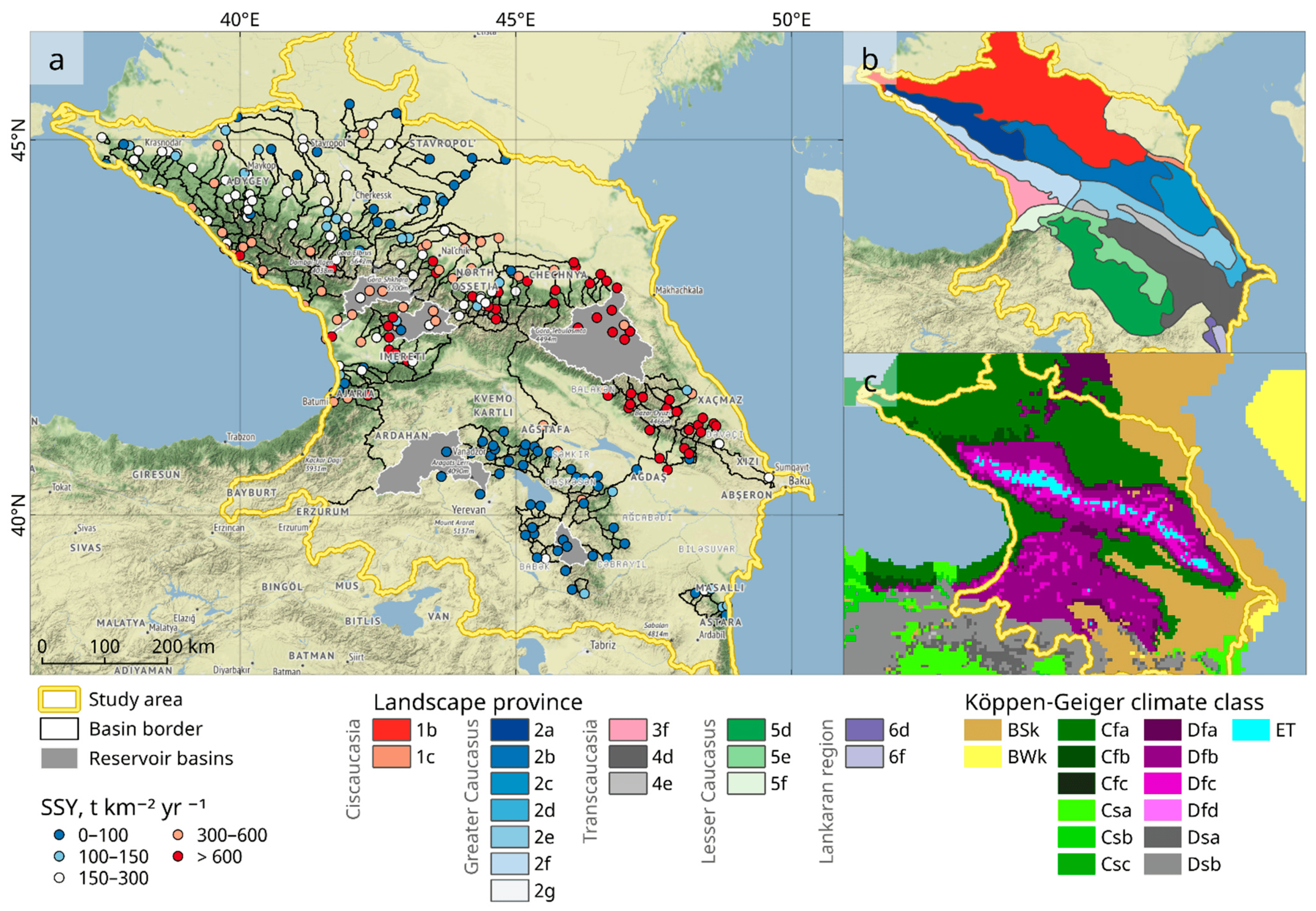
(a) Spatial distribution of gauging stations (GS) used in this study; (b) the main landscape zones and landscape areas of the Caucasus region (modified from [52]). Landscape zones: a–broad-leaved rain barrier, b–steppe, c–semi-desert, d–desert, e–sub-Mediterranean (arid-forest), f–humid subtropical rain-barrier, g–Mediterranean. Landscape areas: 1–Ciscaucasia, 2–Greater Caucasus, 3–Western Transcaucasia (Rioni region), 4–Eastern Transcaucasia (Kura-Araks region), 5–Lesser Caucasus and Armenian Highlands, 6–Lankaran (Elbursk) region; (c) Köppen-Geiger climate classification [51]. Description of Köppen-Geiger climate symbols and defining criteria presented in Supplementary Material. Map tiles by Stamen Design [54].
Figure 1.
(a) Spatial distribution of gauging stations (GS) used in this study; (b) the main landscape zones and landscape areas of the Caucasus region (modified from [52]). Landscape zones: a–broad-leaved rain barrier, b–steppe, c–semi-desert, d–desert, e–sub-Mediterranean (arid-forest), f–humid subtropical rain-barrier, g–Mediterranean. Landscape areas: 1–Ciscaucasia, 2–Greater Caucasus, 3–Western Transcaucasia (Rioni region), 4–Eastern Transcaucasia (Kura-Araks region), 5–Lesser Caucasus and Armenian Highlands, 6–Lankaran (Elbursk) region; (c) Köppen-Geiger climate classification [51]. Description of Köppen-Geiger climate symbols and defining criteria presented in Supplementary Material. Map tiles by Stamen Design [54].

Figure 2.
Suspended sediment yield database overview: boxplots are showing the distribution of reported SSY values by gauging station altitude (a), Köppen-Geiger climate class (c), and Isachenko landscape province (d); SSY measuring period distribution (b).
Figure 2.
Suspended sediment yield database overview: boxplots are showing the distribution of reported SSY values by gauging station altitude (a), Köppen-Geiger climate class (c), and Isachenko landscape province (d); SSY measuring period distribution (b).

Like the climatic and landscape classifications, each basin was also classified into altitude zones depending on the GS elevation (i.e., catchment outlet): Lowlands (0–500 m a.s.l.), Low Mountain Ranges (500–1000 m a.s.l.), Middle Mountain Ranges (1000–1500 m a.s.l.) and High Mountain Ranges (>1500 m a.s.l.).
2.3. Potential Controlling Factors
For every basin, several variables describing the topography, lithology, climate, and other factors that can potentially affect SSY were derived. Table 1 gives an overview of these parameters. Variable values were extracted for each catchment, using catchment boundaries derived from the digital elevation model (DEM). These boundaries and morphometric indices were calculated from the void-filled 30 m ALOS World 3D (AW3D30) DEM by the Japanese Aerospace Exploration Agency (JAXA). Nevertheless, this dataset has had horizontal and vertical errors in the range of tens of meters. It currently offers tremendous potential for regional mountain geomorphological analyses [55]. DEM preprocessing was done in ArcMap ver. 10.8 (http://www.esri.com (accessed on 9 November 2021)) using the Spatial Analyst toolbox.
From preprocessed DEM, we calculated an elevation’s coefficient of variation (DEM [–] in Table 1) by dividing the standard deviation by mean catchment elevation. In line with several other studies focusing on the relation between denudation rates and topography [23,24,49], a normalized steepness index (Ksn [m0.9]) was also calculated. It represents the upstream area-weighted channel gradient [56]:
in which S is the channel slope (m m−1); A is the upstream drainage area (m2); θ is the concavity index set to 0.45 to ease comparisons between streams with differing catchment areas and concavities. We calculated Ksn in MATLAB using the Topo Toolbox Software [57,58].
As a proxy of slope lengths, we used the precalculated height Above the Nearest Drainage (HAND, m) in the MERIT dataset [59]. HAND normalizes DEMs according to distributed vertical distances relative to the drainage channels [60].
In order to assess the potential importance of tectonic activity in explaining the observed SSY variation, we computed the area-weighted average peak ground acceleration with a 10% exceedance probability in 50 years (PGA, m s−2) derived from the GSHAP Global Seismic Hazard dataset [61,62] following the recommendations from Vanmaercke et al. [22].
The global lithological map database (GLiM) [28] and average chemical weathering rates (CWR, t km−2 year−1) calculated for every individual GLiM class by Hartmann et al. [63] were used. The spatial distribution of CWR rates is presented in Supplementary Material. Then for every catchment in our database, the area-weighted average CWR was estimated.
We derived the sand-fraction map based on topsoil (0–30 cm depth) structure from the SoilGrids database [64] at 250 m resolution (Supplementary Material). Therefore, the SAND parameter (see Table 1) represents the average fraction of sand in the first 30 cm of soil.
The authors used several regional studies to assess the fraction of landuse/landcover classes (see Supplementary Material). Thus, cropland, forest, and barren areas for 2015 were calculated based on research by Buchner et al. [65]. The glacier areas for 2014 were derived from the GLIMS database [66]. We also estimated a mean tree canopy height (CANOPY, m) within a catchment as a proxy of forest structure and aboveground biomass. For this purpose, a 30 m global forest canopy height map [67] was used.
Additionally, the fragmentation of landuse/landcover classes within basins was determined using Shannon’s Diversity Index (SHDI) [68]. The SHDI shows the relative profusion of each land cover class and is frequently used as a diversity metric in biodiversity and ecology studies [69,70,71]. The SHDI calculates as follows:
where Pi is the proportion of class i.
This study used mean annual basin-averaged climate parameters calculated from a TerraClimate [72] dataset for 1958–2018. We estimated mean annual precipitation (P, mm), a mean annual air temperature (AET, °C), a mean annual downward solar radiation flux at the surface (SRAD, W m−2), a mean annual cumulative streamflow (Q, mm). We also estimated basin-averaged mean annual rainfall erosivity based on Global Rainfall Erosivity Dataset (GLORED, MJ mm ha−1 h−1 year−1) created by Panagos et al. [73] based on high temporal resolution rainfall records from 3530 stations worldwide.
2.4. Uncertainty Assessment
The errors of the suspended sediment yield values were estimated by taking into account the most important sources of uncertainties. In this research, other potential SSY values were simulated using the following equation, modified from Vanmaercke et al. [18]:
in which SSYcor is a corrected value of SSY after considering the various sources of uncertainty. UME reflects the uncertainties associated with measuring errors; UMP represents the uncertainty associated with the length of the measuring period.
A first significant source of uncertainty (UME) is the effects of various methodological errors during the SSY measurements. The degree of these measuring errors depends on various (unknown) methodological details. In previous studies, it has been reported that these errors are usually 20–30% [18,76,77]. Therefore, we have assumed that 30% gives a realistic and relatively conservative estimate of the SSY-value uncertainty associated with measurement errors. Hence, UME was simulated as a random number from a normal distribution with a mean of 1 and a standard deviation of 0.30.
Uncertainties related to the duration of the measuring period describe interannual sediment export variability. Recent studies by Vanmaercke et al. [78] indicate that Weibull distribution describes such interannual variations in SSY (with a scale of 172.7 and shape 1.22). We selected n values from the median Weibull distribution to simulate UMP with n equal to the measuring period duration. Then we calculated the sample’s mean and divided it by the real average of the Weibull distribution [18]. The average value (24 years) was used when the duration of the measuring period was not available.
Likewise, data derived from global datasets generally have critical errors and uncertainties. We, therefore, try to consider them in this study by applying a simplified version of Equation (4). For every parameter examined as a potential controlling factor (F), we simulate alternative values (Fsim) using the following formula:
in which Uer is the uncertainty associated with dataset errors and accuracies (see Table 1). It was simulated as a random number from a normal distribution with a mean of 1 and a standard deviation of uncertainties from Table 1.
Previously, Boulton and Stokes [55] found that river network derivatives from AW3D30 (2017th release) are highly accurate (even the Ksn). However, there is no data available on relative errors of the AW3D30 river derivatives. The overall elevation accuracy of the AW3D30 DEM was estimated as <3 m by Boulton and Stokes [55] and as <5 m by mission specifications [79]. Previous studies found that the vertical root mean square error was lower (<5 m) in flat areas [80,81] and higher (up to 12–14 m) in mountainous areas [81]. Considering the average elevation difference within the studied watersheds equal to 2700 m and the elevation range for the whole studied region from 0 to 5639 m, we assumed a 1% elevation accuracy is a realistic uncertainty measure. For this study, we hypothesized that river network derivatives from AW3D30 would have the same relative error.
While accuracy assessment has not been previously reported for the HAND dataset, it is known from previous studies that it is mainly controlled by the definition of the accumulated area [60]. As in this study, we derived HAND from the MERIT dataset [59]. Thus, we assumed that uncertainty is attributable to errors in MERIT’s flow accumulation estimates. In most cases, the reported relative error of the accumulation area is <0.05 [59]. There were only a dozen validation stations in the Caucasus region with accumulation area relative error ±5%. Hence, we could estimate the overall uncertainty of the HAND dataset as 5%. However, this value should be used with caution as it does not include uncertainties associated with validation station location, possible hydrologic fluctuations, and unreported HAND model accuracy.
Buchner et al. [65] reported the 2015th landuse map accuracy by classes: 29% for barren areas, 8% for cropland areas, and 15% for forest areas (averaged among various forest types). Therefore, uncertainties of the landcover change associated with measuring errors were simulated as a random number from a normal distribution with a mean of 1 and a standard deviation of 0.29 for barren, 0.8 for cropland, and 0.15 for a forest. Potapov et al. [67] indicated that the accuracy of the canopy tree dataset varies from 83% to 92.9%, depending on the forest class threshold and reference source. We assumed a relative error of 12% provides a realistic estimate of canopy height uncertainty.
Tielidze and Wheate [74], in their study, reported that the accuracy of glacier’s outline identification in 1960 varies between 4.8% and 5.9%. The error was associated with mapping and georeferencing errors. We used a 5% value as an uncertainty measure.
Shedlock et al. [62] provided no further details on the accuracy of the PGA map. Seeing that that map has a probabilistic nature of hazard analyses makes it hard to validate [82]. Nevertheless, the relative error of the estimated peak ground acceleration should likely be about 20% since some studies [83] indicate that this is the percentage of large earthquakes that are not predicted.
Equations (4) and (5) were used to simulate 1000 alternative SSY and controlling factors for every basin. We calculated 95% confidence intervals on every SSY value (i.e., the difference between the 97.5% and 2.5% quantile of the 1000 simulated values).
2.5. Statistical Analyses
The relative importance of control variables in explaining SSY was assessed through partial correlation analyses (using the Spearman rank test). All statistical analysis was done in R 4.1.0 [84] unless otherwise noted.
The partial least squares regression (PLSR) technique was also used to analyze the relationship between SSY and controlling factors. This method combines Principal Component Analysis (PCA) and Multiple Linear Regression [85,86]. The PLSR model is based on a linear combination of the original scores that aim at the best representation of the response variable [87], i.e., suspended sediment yield. One of the strengths of the PLSR over the PCA is that both quantitative and qualitative variables can be used to explain the dependent variables. The Q2 (i.e., the cross-validated R2) index was used to assess the PLSR model quality [85]. The Q2 represents the global component contribution and determines the most stable model when close to 1. Applying this goodness of prediction estimator is very common in PLSR models studies [85,87,88,89].
There were two models run with various sets of explanatory variables. Model A was based only on numeric variables (see Table 1, everything except KG and LZ). In contrast, in Model B, we added qualitative (dummy) variables such as climatic region (KG) and landscape zone (LZ).
We applied variable importance in the PLSR projection (VIP) filter measure to select the most relevant variables. The authors used a VIP value threshold equal to 1, suggesting that variables with VIP higher than 1 are essential in explaining SSY [90]. We performed the PLSR analysis using the XLSTAT ver. 2021.3.1 software by Addinsoft.
3. Results
3.1. Database Overview
Table 2 gives descriptive statistics of collected data. The observed mean annual suspended sediment yield in the Caucasus region is 426 ± 71.9 t km−2 year−1. It varies from 5 to 4100 t km−2 year−1. The map presented in Figure 1a can reveal some general patterns of SSY in the Caucasus region. The map shows that low SSY values generally characterize large parts of the Lesser Caucasia and Ciscaucasia (<100–150 t km−2 year−1). While in the Greater Caucasus, values higher than 150 t km−2 year−1 and even above 300 t km−2 year−1 are a lot more frequent. Furthermore, the western part and the high mountain belt of the Greater Caucasus can be clearly distinguished by values above 600 t km−2 year−1.
Figure 1b displays the distribution of SSY per climate class, while Table 2 reports descriptive statistics of the SSY-values per climate class. This comparison indicates some apparent differences: the Dfc climate type (snow climate, fully humid with cold summer) has the highest SSY values, it is significantly (p < 0.00008) higher than the most common Dfb class (snow climate, fully humid with warm summer) and the Cfa (warm temperate climate, fully humid with hot summer). The ET regions have intermediate values. For other classes, the number of observations is too low to draw any conclusions.
Grouping SSY entries by landscape provinces reveals much more SSY distribution diversity (see Figure 2d). Thus, SSY in 2c and 2e provinces (eastern part of the Greater Caucasus) is the highest in the region. Conducted pairwise Wilcoxon rank-sum test revealed that mean SSY values in the eastern part (landscape zone 2e and 2c) of the Great Caucasus are significantly (p < 0.002) higher than in the western (2f and 2a). We observe the lowest SSY values in the Lesser Caucasus (5d–f), while the central part of the Greater Caucasus (2b) generally has the intermediate values.
Once the SSY data are aggregated by altitude zone (Figure 2a, Table 2), the findings suggest that SSY distribution for lowland basins (GS altitude < 500 m a.s.l.) is overall lower than the SSY distribution for mountain catchments. Low mountain catchments (500–1000 m a.s.l.) also have lower SSY values than middle and high mountain ranges. However, all these differences are not significant according to the Wilcoxon rank-sum test.
3.2. Correlation Analyses
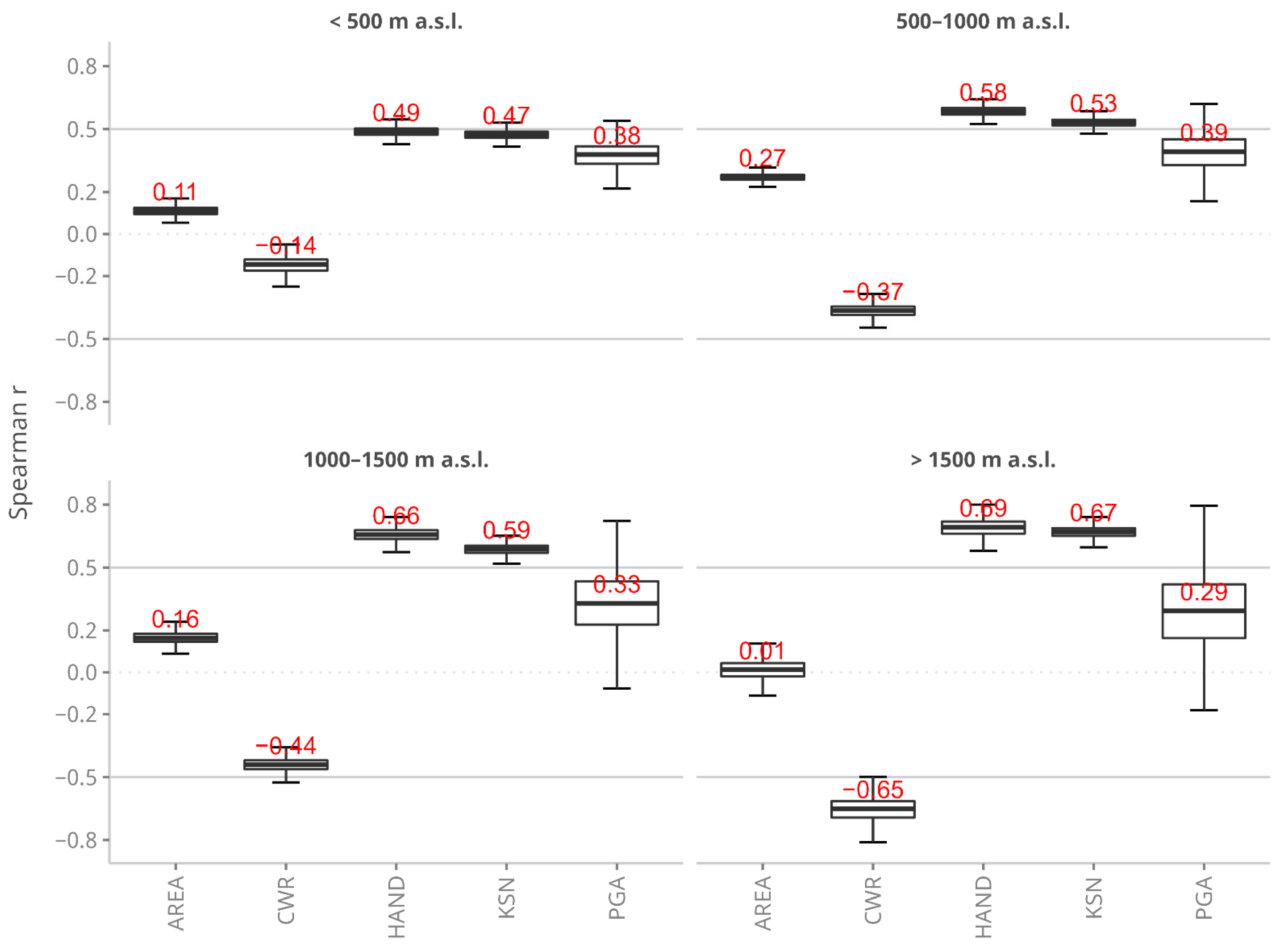
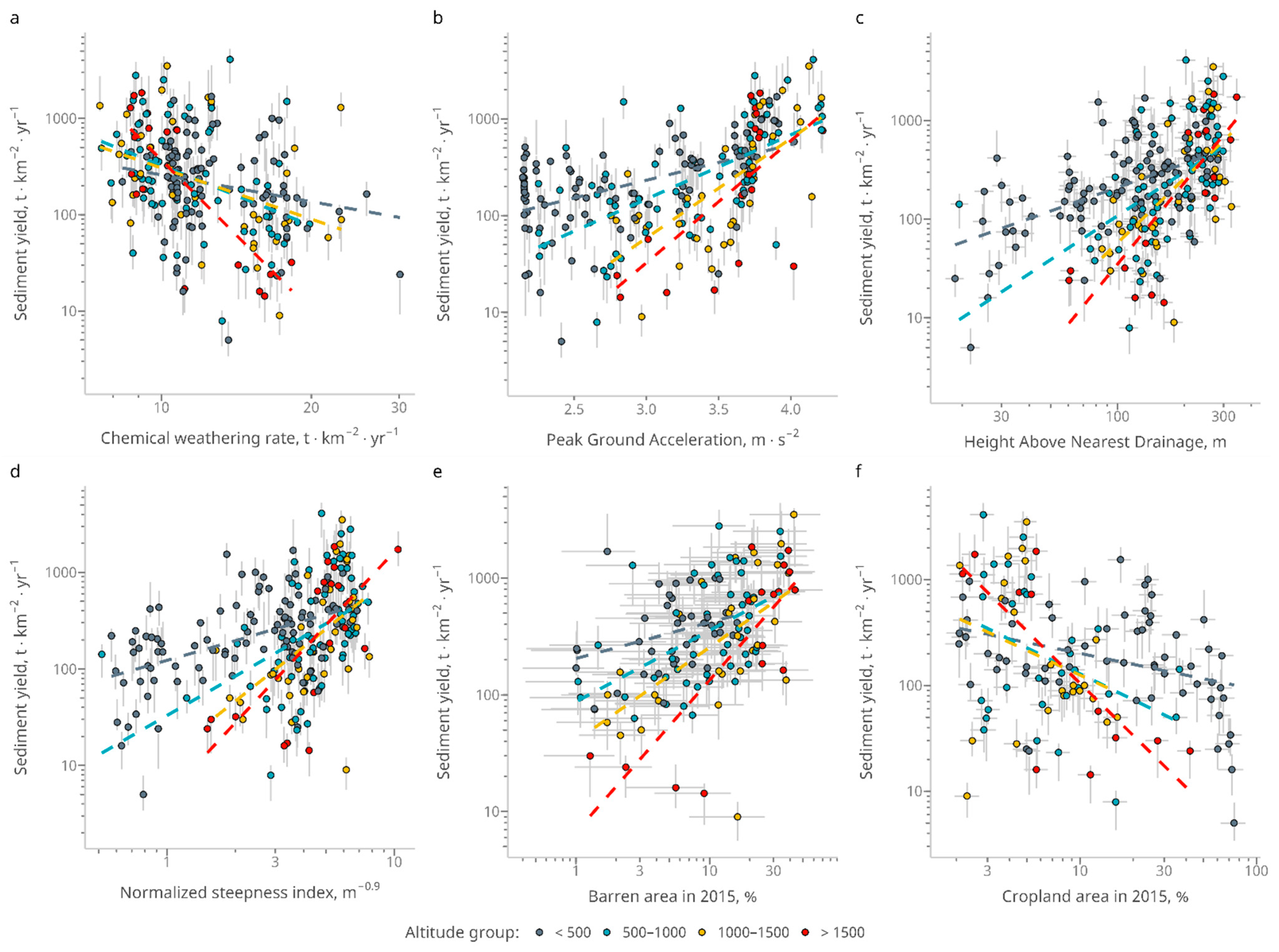
Table 3 shows the partial correlations between all considered variables and SSY. The partial correlation analyses indicate that catchment sediment yields are mainly controlled by HAND, Ksn, and the contemporary fraction of barren land (Barren). We observe a negative correlation between the SSY and the CWR (Spearman r = −0.37, CI = [−0.4; −0.33]). However, the further study points to differences depending on the altitude zone (Figure 3, Figure 4 and Figure 5). Therefore, if we consider only the high mountain ranges (>1500 m) catchments, there is a highly significant negative correlation between SSY and CWR (Spearman r = −0.65). The CWR explains 64% of the variation in SSY of high mountain catchments (Figure 6d).
3.3. Partial Least Squares Analyses
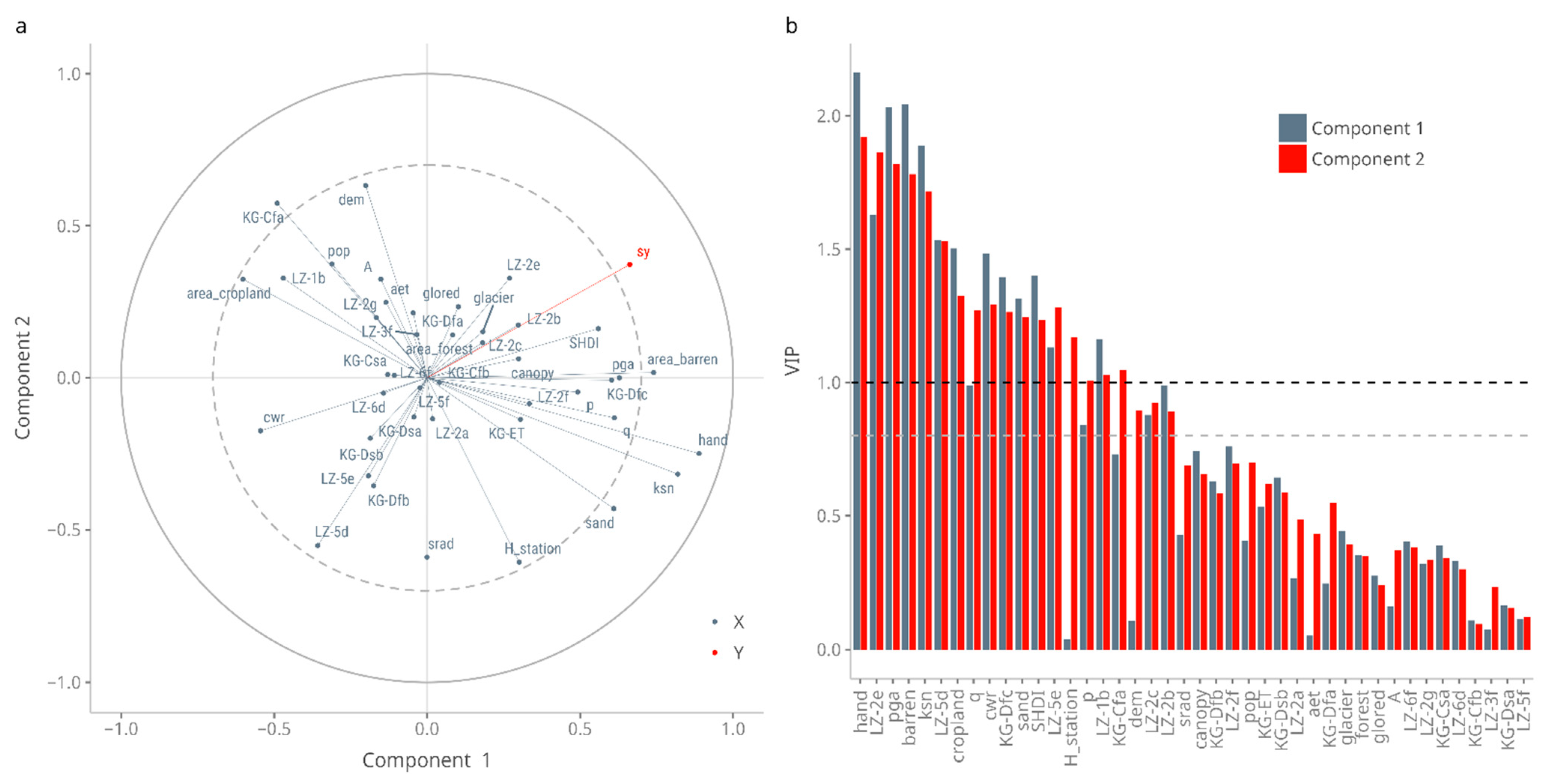
To visualize the multidimensional data structure between controlling variables (see Table 1), a biplot of scores and correlation loadings was constructed based on a PLSR model B (Figure 7a). The plot graphically summarizes which of the factors controls SSY. In component 1, 15% of the explanatory variables (X) variance was used to explain 43.8% of the response variables (Y) variance. In component 2, 23.1% of the variance of the controlling factors was used to explain 57.7% of the SSY variance. A measure of goodness of prediction Q2 showed that component 1 and component 2 almost equally contribute to the model B quality (40.7% and 49.3%, respectively). Among factors controlling the SSY, the HAND and Ksn values were highly positively correlated (r = −0.95, p < 0.001) (Figure 7a). Suspended sediment yield was generally less associated with catchment area (r = 0.13 p = 0.04) and rainfall erosivity (r = 0.16 p = 0.01). Whereas forest fraction (FOREST) and mean annual temperature (AET) appeared not to be statistically significant factors (p > 0.05). Important explanatory variables (VIP > 1) in the projection for SSY (Figure 7b) created the following decreasing order: HAND > LZ > PGA > BARREN > Ksn > Cropland > Q > CWR > KG > SAND > SHDI.
Adding extra dummy variables (climate region and landscape province) made it possible to describe 10% more variation of the SSY (Table 4) with the same number of components. However, the overall quality of the model (Q2) does not change significantly.
4. Discussion
4.1. SSY Overview
To the authors’ knowledge, a database used in this research is currently the most extensive and detailed database of suspended sediment yield measurements in the Caucasus. However, we are aware that much more SSY data probably exists that is not included in this analysis. For example, the gauging station density in Transcaucasia (i.e., Georgia, Azerbaijan, and Armenia) is low, while earlier studies [41,91] indicate that there are some more GS exist.
Overall, the average SSY (426 t km−2 year−1) agrees well with the average SSY of the European Alps (451 t km−2 year−1 [15]). Earlier estimates of the denudation rates in the Caucasus region suggest a mean annual denudation rate of 0.2 mm year−1 [91]. More recent estimates imply that the mean annual denudation rate should range from 0.005 to 2.32 mm year−1 [41]. Mozzherin and Sharifullin [41] calculated denudation rates (hc, mm year−1) using the following equation:
in which SSY is a suspended sediment yield [t km−2 year−1]. Equation (6) was further used to compare this study’s results with previous findings. As such, the mean denudation rate for the Caucasus region based on this study database is 0.16 ± 0.027 mm year−1 with a maximum of 1.55 mm year−1. These values are in line with previous studies [41,91]. As indicated by Figure 1, the spatial patterns of our study correspond relatively well with those estimated by Mozzherin and Sharifullin [41]. However, these values should not be treated as actual denudation rates as the equation used (Equation (6)) to obtain them does not incorporate the bedload sediment transport. While the bedload fraction in mountain rivers can be 20–40% from total sediment load on average [92,93,94], it may increase up to 90–99% in some years [95].
4.2. Controlling Factors
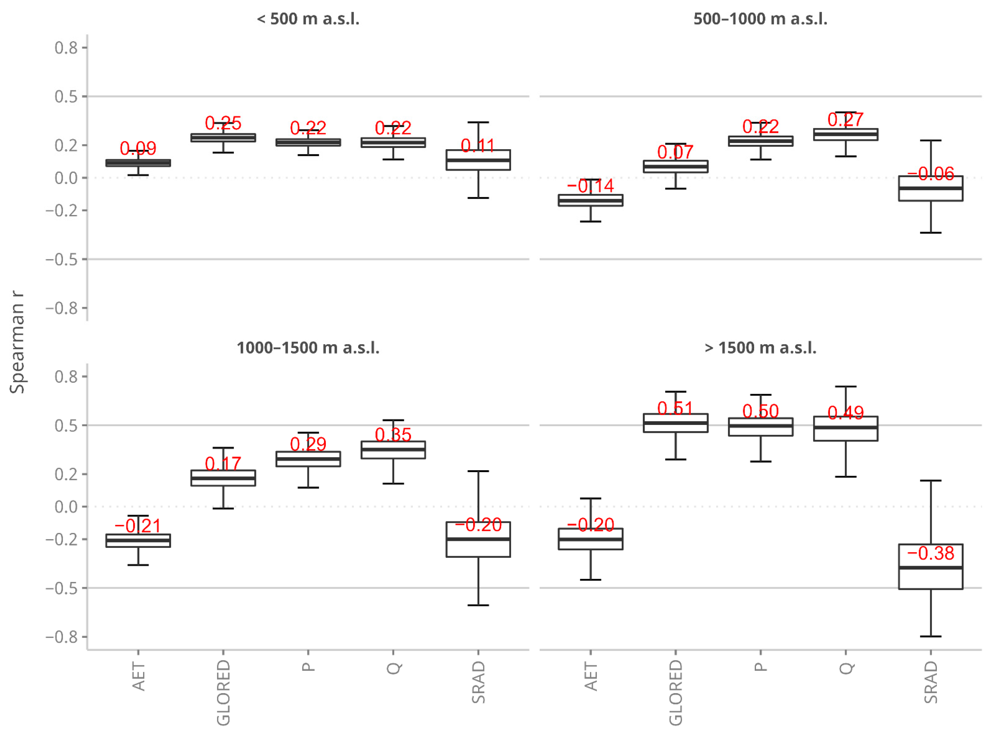
We found that SSY distribution differs less between altitude zones than climatic regions and landscape provinces (Figure 1). These findings are in line with Vanmaercke et al. [15]. They found that hilly catchments (<500 m a.s.l.) generally have lower SSY values, while other differences between mountain ranges are insignificant. While the SSY distribution within landscape provinces (Figure 2d) may somehow repeat general spatial climate patterns for the Caucasus [43,44], a closer look at the relationships between climate factors and SSY does not reveal any strong explaining power (Table 3, Figure 5 and Figure 7). On the one hand, this is reasonably expected considering previous findings [22,34]. On the other, the sediment yield in mountain areas is mainly formed during the snow melting or rainfall [13,14], which can also lead to the formation of landslides, rainfall-driven floods, and glacier lake outburst floods [96,97]. Meanwhile, moraine deposits, traces of the Last Glacial Maximum [98], are actively eroded by streams at any water level rise, similar to that observed in the Rocky Mountains of eastern Canada [99]. Additional friable material is regularly exported by the first-second order tributaries (Horton system) to the bottoms of higher-order valleys with debris- and mudflows. For example, the modern sedimentation rate in the bottom of the Baksan river (North Caucasus) valley reaches tens of centimeters per year [100].
The most robust relationship was found between the SSY and topographic factors (Figure 3 and Figure 6), which is easily explained by the latter’s close relationship with river water discharge. Hillslope erosion is also controlled mainly by topographic variables such as height above the nearest drainage (HAND) and normalized steepness index (Ksn). However, it is well known that water discharges primarily determine the mountain river’s sediment loads since streambank erosion is important in total load [101]. Nevertheless, a normalized steepness index corresponds to a more pronounced topography of the catchment area and, hence, higher erosion from slopes [102]. Notably, the non-linear increase of suspended sediment yield with basin average Ksn (Figure 6d) appears to be consistent with the expectation from fluvial incision models [24,103].
The peak ground acceleration (PGA) significantly impacts the SSY in the Caucasus region since this territory belongs to the area of alpine folding. Noticeable movements of the Earth’s crust constantly occur, which provokes mass movements and other slope processes. In general, the tectonics influence on the relief formation of the Caucasus region and denudation is currently much more significant than the climate impact [104].
A close relationship has been established between SSY and chemical weathering rate (CWR) only for basins in the high-mountain belt of the Caucasus region (see Figure 3). It generally agrees with the known concepts like when the threshold value in the denudation rate is reached, the contribution of chemical weathering begins to decrease with a denudation increase [105]. Namely, this is observed in the high mountain belt of the Caucasus, where the maximum SSYs are observed in proglacial rivers, sometimes exceeding the sediment load of similar rivers in other mountainous regions [13].
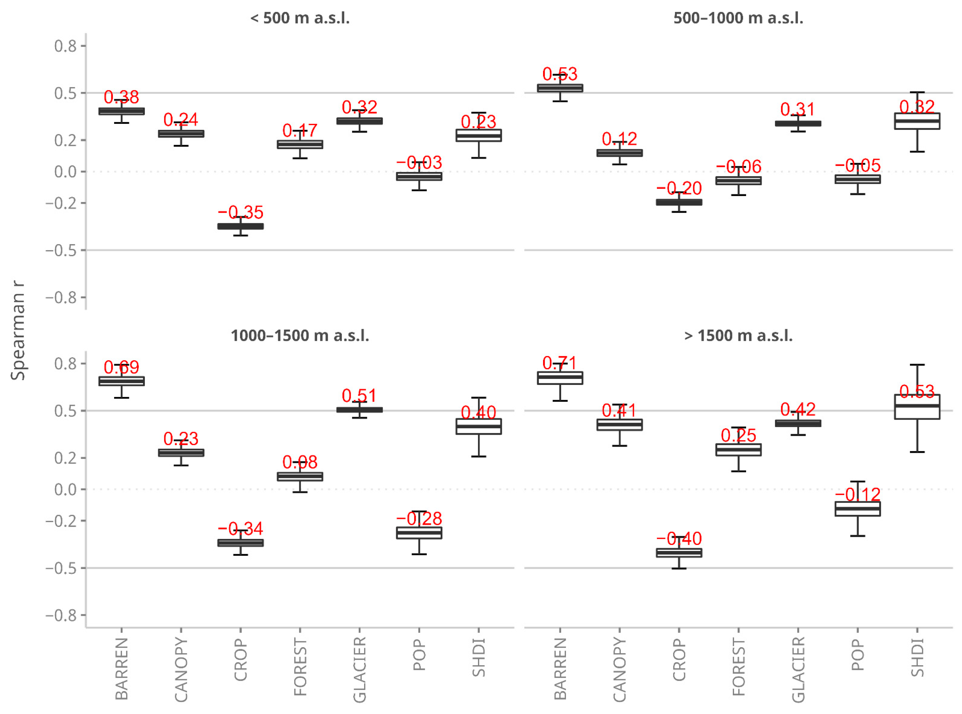
The most significant anthropogenic impact on SSY values could be expected in the hilly and lowland zones of the Caucasus region. This area is characterized by the maximum agricultural development of the territory and, consequently, the highest soil erosion rates on cropland for the European part of Russia [106,107]. However, the performed analysis does not reveal the presence of a close relationship between SSY and cropland area for given zones (Figure 6f). There are several reasons for this. Firstly, most rivers flowing in the hilly and lowland zones originate in the middle and high mountains, and most of the water is formed there. As a result, the share contribution of sediments from plains and foothills differs between basins, depending on the catchment areas’ ratio in various elevation zones. Secondly, in the foothill and lowland zones, rainstorm soil erosion dominates. The sediment delivery ratio varies greatly depending on the length of the dry valley network [108] and the presence of other sediment traps in the catchment.
Thirdly, during extreme floods with low recurrence, which account for the bulk of the suspended sediment yield in mountain river basins [109], a significant part of the transported sediment is redeposited in the bottoms of river valleys within the foothill sections of their channels [100,110]. This is due to a sharp drop in slope steepness and the transport capacity of streams. It also has the most significant impact on the high variability of relationships between sediment yield in the foothills and plain zones of the Caucasus region and the other controlling factors. On the other hand, a reasonably close negative relationship between the cropland area and SSY was established for river basins in the high mountain zone (see Figure 6f). This is because croplands occupy the expansions of the valley bottoms in this zone and serve as sinks for sediments eroded from valley slopes.
Among other factors for all basins of the Caucasus region, a reasonably strong relationship was revealed between SSY and the proportion of barren lands (Figure 6e). This is also expected since barren lands, including badlands, are the primary sediment sources for areas slightly disturbed by humans [111]. Moreover, a good relationship between SSY and the fraction of barren lands is observed for all high-altitude zones. Barren lands are usually located close to streams, or their fraction is quite significant, as is observed in the mountains of Dagestan (Eastern Caucasus), where badlands distribution is associated with the destruction of the soil cover due to overgrazing [112].
The PLSR analyses revealed interdependencies between various explanatory parameters (Figure 7). Thus, the PGA was likely a controlling parameter of the Ksn and HAND, affecting the fraction of barren lands. While a fraction of cropland is somehow positively correlated with the population density, suggesting that arable lands are usually located near settlements. Surprisingly, we did not find any close relationship between rainfall erosivity (GLORED) and SSY values (see Figure 5) for hilly and low mountains catchments where a significant part of sediments should be formed by soil erosion [106]. Contrariwise, a high correlation between GLORED and SSY was observed for high-altitude basins (r = 0.51). This and the interdependency of GLORED with elevation covariates (DEM, GS elevation, see Figure 7) indicate that a possible impact of rainfall erosivity is associated with an elevation used to interpolate WorldClim data [113] used to create GLORED dataset [73]. Another possible explanation is the scarcity of meteorological stations in the mid-mountain and high-mountain belts of the Caucasus Mountains. In this regard, the reliability of the spatial variability of rainfall erosivity and its changes with altitude is generally relatively low.
4.3. Uncertainties and Further Implications
As a result of the uncertainties associated with the reported SSY data (see Section 2.4), our results should be interpreted carefully. Vanmaercke et al. [15] suggested that total uncertainties may be over 100% for some SSY measurements based on their overview of European sediment yield. Inaccurate SSY data measurements could partly explain some poor correlations (see Table 3, Figure 3, Figure 4 and Figure 5). Nevertheless, considering various sources of uncertainties for both SSY and explanatory variables, high correlations with topographic and landuse factors reported here should be realistic.
It is worth noting that the relatively low correlation coefficients and quality indexes are expected in SSY studies [15,18,114,115]. Such low performance can be likely explained by uncertainties in SSY values (see Section 2.4), as our research was based on a similar empirical approach.
The SSY modeling was not the goal of this study; here, on the contrary, we only suggested variables that can be further used in the models. Nevertheless, a preliminary run of the PLSR showed that qualitative variables significantly increase the model’s predictive power (Table 4). Therefore, adding dummy variables such as ecological zones or landscape provinces should be recommended for further studies.
5. Conclusions
Suspended sediment yield (SSY) in various environments has been studied for a long time, but SSY in the Caucasus region has received only limited attention. This study aimed to address this research gap by first exploring an extensive database of measured SSY data. Despite potentially significant uncertainties on SSY measurements and controlling factors, it is possible to point out major regional differences in SSY. Therefore, most catchments in the Lesser Caucasia and Ciscaucasia are characterized by relatively low SSY values (<100–150 t km−2 year−1), the Greater Caucasus region generally have higher SSY values (more than 150–300 t km−2 year−1). As these differences are based on extensive observations, they cannot be attributed to uncertainties in the available data. However, they must result from regional variation of the controlling factors of SSY and different dominant erosion processes.
Based on the exploratory analyses presented here, the particular importance of the various potential controlling factors of SSY could not be determined. We found that such proxies of topography as height above nearest drainage (HAND), normalized steepness index (Ksn) tend to be among the most important ones. However, a PLSR analysis suggested that these variables’ influence is likely associated with peak ground acceleration (PGA) but much easier to measure. We also reveal a strong relationship between various land cover types (e.g., barren areas and cropland) in different elevation zones. We did not aim to create a tool to predict SSY in the Caucasus region. However, our research suggested that including such factors as HAND, Ksn, a fraction of barren and cropland areas in models may be essential to shed some light on the SSY spatial and temporal patterns.
This line of investigation is continuing, looking at a broader range of data and such questions as possible relationships between SSY and natural or anthropogenic control factors and motifs involving their combinations. Using landscape provinces and other qualitative variables as controlling factors in line with PLSR modeling is also an intriguing possibility. In addition, the use of such models to predict suspended sediment yield is of great practical interest, especially in tectonically active regions.
Supplementary Materials
The following are available online at https://www.mdpi.com/article/10.3390/w13223173/s1, Figure S1: Spatial distribution of SSY factors: (a) estimated peak ground acceleration (PGA, m s−2) with an exceedance probability of 10% in 50 years, as derived from the GSHAP data set [61]; (b) average chemical weathering rates (CWR, t km−2 year−1) calculated for every individual GLiM [28] class by Hartmann et al. [63]; (c) Caucasus land-cover classification for 2015 derived from Buchner et al. [65]; (d) mean sand content (SAND, %) in the intrinsic topsoil (0–30 cm depth) from the International Soil Reference and Information Centre (ISRIC) SoilGrids database [64], Table S1: Description of Köppen-Geiger climate symbols and defining criteria.
Author Contributions
Conceptualization, V.G. and A.T.; methodology, A.T.; software, A.T.; formal analysis, A.T. and V.G.; writing—original draft preparation, A.T.; writing—review and editing, V.G.; visualization, A.T.; supervision, V.G.; project administration, V.G.; funding acquisition, V.G. All authors have read and agreed to the published version of the manuscript.
Funding
This work was conducted with support from the ongoing Russian Science Foundation project No. 19-17-00181: “Quantitative assessment of the slope sediment flux and its changes in the Holocene for the Caucasus mountain rivers”. This study contributes to the State Task No. 0148- 2019-0005 (Institute of Geography, Russian Academy of Science) and State Task No. 121051100166-4 (Laboratory of soil erosion and fluvial processes, Faculty of Geography, Lomonosov Moscow State University). Tsyplenkov A. performed this research according to the Development program of the Interdisciplinary Scientific and Educational School of M.V. Lomonosov Moscow State University «Future Planet and Global Environmental Change».
Institutional Review Board Statement
Not applicable.
Informed Consent Statement
Not applicable.
Data Availability Statement
Reproducible R code and data are available at the GitHub repository (https://github.com/atsyplenkov/caucasus-sediment-yield2021 (accessed on 9 November 2021)). Contact Anatoly Tsyplenkov ([email protected]) for more information.
Acknowledgments
The authors acknowledge the core team of the R statistical software for providing a suite of functionalities.
Conflicts of Interest
The authors declare no conflict of interest.
References
- Issaka, S.; Ashraf, M.A. Impact of Soil Erosion and Degradation on Water Quality: A Review. Geol. Ecol. Landsc. 2017, 1, 1–11. [Google Scholar] [CrossRef] [Green Version]
- Evans, A.E.; Mateo-Sagasta, J.; Qadir, M.; Boelee, E.; Ippolito, A. Agricultural Water Pollution: Key Knowledge Gaps and Research Needs. Curr. Opin. Environ. Sustain. 2019, 36, 20–27. [Google Scholar] [CrossRef]
- Owens, P.N. Soil Erosion and Sediment Dynamics in the Anthropocene: A Review of Human Impacts during a Period of Rapid Global Environmental Change. J. Soils Sediments 2020, 20, 4115–4143. [Google Scholar] [CrossRef]
- Alewell, C.; Ringeval, B.; Ballabio, C.; Robinson, D.A.; Panagos, P.; Borrelli, P. Global Phosphorus Shortage Will Be Aggravated by Soil Erosion. Nat. Commun. 2020, 11, 4546. [Google Scholar] [CrossRef] [PubMed]
- Beusen, A.H.W.; Dekkers, A.L.M.; Bouwman, A.F.; Ludwig, W.; Harrison, J. Estimation of Global River Transport of Sediments and Associated Particulate C, N, and P. Glob. Biogeochem. Cycles 2005, 19, GB4S05. [Google Scholar] [CrossRef]
- Bouwman, A.F.; Beusen, A.H.W.; Billen, G. Human Alteration of the Global Nitrogen and Phosphorus Soil Balances for the Period 1970–2050. Glob. Biogeochem. Cycles 2009, 23, GB0A04. [Google Scholar] [CrossRef]
- Richards, K. Drainage Basin Structure, Sediment Delivery and the Response to Environmental Change. Geol. Soc. Lond. Spec. Publ. 2002, 191, 149–160. [Google Scholar] [CrossRef]
- Najafi, S.; Dragovich, D.; Heckmann, T.; Sadeghi, S.H. Sediment Connectivity Concepts and Approaches. Catena 2021, 196, 104880. [Google Scholar] [CrossRef]
- Mano, V.; Nemery, J.; Belleudy, P.; Poirel, A. Assessment of Suspended Sediment Transport in Four Alpine Watersheds (France): Influence of the Climatic Regime. Hydrol. Process. 2009, 23, 777–792. [Google Scholar] [CrossRef]
- Gusarov, A.V.; Sharifullin, A.G.; Komissarov, M.A. Contemporary Long-Term Trends in Water Discharge, Suspended Sediment Load, and Erosion Intensity in River Basins of the North Caucasus Region, SW Russia. Hydrology 2021, 8, 28. [Google Scholar] [CrossRef]
- Tsyplenkov, A.S.; Golosov, V.N.; Belyakova, P.A. How Did the Suspended Sediment Load Change in the North Caucasus during the Anthropocene? Hydrol. Process. 2021, 35, e14403. [Google Scholar] [CrossRef]
- Tsyplenkov, A.; Vanmaercke, M.; Golosov, V. Contemporary Suspended Sediment Yield of Caucasus Mountains. Proc. Int. Assoc. Hydrol. Sci. 2019, 381, 87–93. [Google Scholar] [CrossRef] [Green Version]
- Tsyplenkov, A.; Vanmaercke, M.; Golosov, V.; Chalov, S. Suspended Sediment Budget and Intra-Event Sediment Dynamics of a Small Glaciated Mountainous Catchment in the Northern Caucasus. J. Soils Sediments 2020, 20, 3266–3281. [Google Scholar] [CrossRef]
- Tsyplenkov, A.; Vanmaercke, M.; Collins, A.L.; Kharchenko, S.; Golosov, V. Elucidating Suspended Sediment Dynamics in a Glacierized Catchment after an Exceptional Erosion Event: The Djankuat Catchment, Caucasus Mountains, Russia. Catena 2021, 203, 105285. [Google Scholar] [CrossRef]
- Vanmaercke, M.; Poesen, J.; Verstraeten, G.; de Vente, J.; Ocakoglu, F. Sediment Yield in Europe: Spatial Patterns and Scale Dependency. Geomorphology 2011, 130, 142–161. [Google Scholar] [CrossRef] [Green Version]
- Cohen, S.; Kettner, A.J.; Syvitski, J.P.M.; Fekete, B.M. WBMsed, a Distributed Global-Scale Riverine Sediment Flux Model: Model Description and Validation. Comput. Geosci. 2013, 53, 80–93. [Google Scholar] [CrossRef]
- Poesen, J. Soil Erosion in the Anthropocene: Research Needs: Soil Erosion in the Anthropocene. Earth Surf. Process. Landf. 2018, 43, 64–84. [Google Scholar] [CrossRef]
- Vanmaercke, M.; Poesen, J.; Govers, G.; Verstraeten, G. Quantifying Human Impacts on Catchment Sediment Yield: A Continental Approach. Glob. Planet. Chang. 2015, 130, 22–36. [Google Scholar] [CrossRef]
- Milliman, J.D.; Syvitski, J.P.M. Geomorphic/Tectonic Control of Sediment Discharge to the Ocean: The Importance of Small Mountainous Rivers. J. Geol. 1992, 100, 525–544. [Google Scholar] [CrossRef]
- Higgitt, D.L.; Lu, X.X. Sediment Delivery to the Three Gorges: 1. Catchment Controls. Geomorphology 2001, 41, 143–156. [Google Scholar] [CrossRef]
- Syvitski, J.P.M.; Milliman, J.D. Geology, Geography, and Humans Battle for Dominance over the Delivery of Fluvial Sediment to the Coastal Ocean. J. Geol. 2007, 115, 1–19. [Google Scholar] [CrossRef] [Green Version]
- Vanmaercke, M.; Kettner, A.J.; Eeckhaut, M.V.D.; Poesen, J.; Mamaliga, A.; Verstraeten, G.; Rãdoane, M.; Obreja, F.; Upton, P.; Syvitski, J.P.M.; et al. Moderate Seismic Activity Affects Contemporary Sediment Yields. Prog. Phys. Geogr. Earth Environ. 2014, 38, 145–172. [Google Scholar] [CrossRef] [Green Version]
- Vanacker, V.; von Blanckenburg, F.; Govers, G.; Molina, A.; Campforts, B.; Kubik, P.W. Transient River Response, Captured by Channel Steepness and Its Concavity. Geomorphology 2015, 228, 234–243. [Google Scholar] [CrossRef] [Green Version]
- DiBiase, R.A.; Whipple, K.X.; Heimsath, A.M.; Ouimet, W.B. Landscape Form and Millennial Erosion Rates in the San Gabriel Mountains, CA. Earth Planet. Sci. Lett. 2010, 289, 134–144. [Google Scholar] [CrossRef]
- Campforts, B.; Schwanghart, W.; Govers, G. Accurate Simulation of Transient Landscape Evolution by Eliminating Numerical Diffusion: The TTLEM 1.0 Model. Earth Surf. Dyn. 2017, 5, 47–66. [Google Scholar] [CrossRef] [Green Version]
- Schwanghart, W.; Kuhn, N.J. TopoToolbox: A Set of Matlab Functions for Topographic Analysis. Environ. Model. Softw. 2010, 25, 770–781. [Google Scholar] [CrossRef]
- Kober, F.; Zeilinger, G.; Hippe, K.; Marc, O.; Lendzioch, T.; Grischott, R.; Christl, M.; Kubik, P.W.; Zola, R. Tectonic and Lithological Controls on Denudation Rates in the Central Bolivian Andes. Tectonophysics 2015, 657, 230–244. [Google Scholar] [CrossRef] [Green Version]
- Hartmann, J.; Moosdorf, N. The New Global Lithological Map Database GLiM: A Representation of Rock Properties at the Earth Surface. Geochem. Geophys. Geosyst. 2012, 13. [Google Scholar] [CrossRef]
- Korup, O. Rock Type Leaves Topographic Signature in Landslide-Dominated Mountain Ranges. Geophys. Res. Lett. 2008, 35. [Google Scholar] [CrossRef] [Green Version]
- Portenga, E.W.; Bierman, P.R. Understanding Earth’s Eroding Surface with 10Be. GSA Today 2011, 21, 4–10. [Google Scholar] [CrossRef]
- Molnar, P.; Anderson, R.S.; Anderson, S.P. Tectonics, Fracturing of Rock, and Erosion. J. Geophys. Res. Earth Surf. 2007, 112, F03014. [Google Scholar] [CrossRef]
- Vanmaercke, M.; Obreja, F.; Poesen, J. Seismic Controls on Contemporary Sediment Export in the Siret River Catchment, Romania. Geomorphology 2014, 216, 247–262. [Google Scholar] [CrossRef] [Green Version]
- Vanmaercke, M.; Ardizzone, F.; Rossi, M.; Guzzetti, F. Exploring the Effects of Seismicity on Landslides and Catchment Sediment Yield: An Italian Case Study. Geomorphology 2017, 278, 171–183. [Google Scholar] [CrossRef]
- Nadal-Romero, E.; Martínez-Murillo, J.F.; Vanmaercke, M.; Poesen, J. Scale-Dependency of Sediment Yield from Badland Areas in Mediterranean Environments. Prog. Phys. Geogr. Earth Environ. 2011, 35, 297–332. [Google Scholar] [CrossRef]
- Jeffery, M.L.; Yanites, B.J.; Poulsen, C.J.; Ehlers, T.A. Vegetation-Precipitation Controls on Central Andean Topography. J. Geophys. Res. Earth Surf. 2014, 119, 1354–1375. [Google Scholar] [CrossRef] [Green Version]
- Carretier, S.; Regard, V.; Vassallo, R.; Aguilar, G.; Martinod, J.; Riquelme, R.; Pepin, E.; Charrier, R.; Hérail, G.; Farías, M.; et al. Slope and Climate Variability Control of Erosion in the Andes of Central Chile. Geology 2013, 41, 195–198. [Google Scholar] [CrossRef]
- Hallet, B.; Hunter, L.; Bogen, J. Rates of Erosion and Sediment Evacuation by Glaciers: A Review of Field Data and Their Implications. Glob. Planet. Chang. 1996, 12, 213–235. [Google Scholar] [CrossRef]
- Hoffmann, T.; Thorndycraft, V.R.; Brown, A.G.; Coulthard, T.J.; Damnati, B.; Kale, V.S.; Middelkoop, H.; Notebaert, B.; Walling, D.E. Human Impact on Fluvial Regimes and Sediment Flux during the Holocene: Review and Future Research Agenda. Glob. Planet. Chang. 2010, 72, 87–98. [Google Scholar] [CrossRef]
- Gyssels, G.; Poesen, J.; Bochet, E.; Li, Y. Impact of Plant Roots on the Resistance of Soils to Erosion by Water: A Review. Prog. Phys. Geogr. Earth Environ. 2005, 29, 189–217. [Google Scholar] [CrossRef] [Green Version]
- Vanacker, V.; von Blanckenburg, F.; Govers, G.; Molina, A.; Poesen, J.; Deckers, J.; Kubik, P. Restoring Dense Vegetation Can Slow Mountain Erosion to near Natural Benchmark Levels. Geology 2007, 35, 303–306. [Google Scholar] [CrossRef]
- Mozzherin, V.V.; Sharifullin, A.G. Estimation of Current Denudation Rate of the Mountains Based on the Suspended Sediment Runoff of the Rivers (the Tien Shan, the Pamir-Alai, the Caucasus, and the Alps as an Example). Geomorphol. RAS 2015, 1, 15–23. [Google Scholar] [CrossRef]
- Stokes, C.R. Caucasus Mountains. In Encyclopedia of Snow, Ice and Glaciers; Singh, V.P., Singh, P., Haritashya, U.K., Eds.; Springer: Dordrecht, The Netherlands, 2011; pp. 127–128. ISBN 978-90-481-2642-2. [Google Scholar]
- Horvath, E.; Field, W.O.; Field, W.O. The Caucasus. In Mountain Glaciers of the Northern Hemisphere; Corps of Engineers, US Army, Technical Information Analysis Center, Cold Regions Research and Engineering Laboratory: Hanover, NH, USA, 1975. [Google Scholar]
- Volodicheva, N. The Caucasus. In The Physical Geography of Northern Eurasia; Shahgedanova, M., Ed.; Oxford University Press: Oxford, UK, 2002; pp. 350–376. [Google Scholar]
- Hinderer, M.; Kastowski, M.; Kamelger, A.; Bartolini, C.; Schlunegger, F. River Loads and Modern Denudation of the Alps—A Review. Earth-Sci. Rev. 2013, 118, 11–44. [Google Scholar] [CrossRef]
- Dedkov, A.P.; Moszherin, V.I. Erosion and Sediment Runoff on the Earth; Izd-vo Kazansk. un-ta: Kazan, Russia, 1984; p. 264. [Google Scholar]
- Dedkov, A.P.; Moszherin, V.I. Erosion and Sediment Yield in Mountain Regions of the World. Eros. Debris Flows Environ. Mt. Reg. 1992, 209, 29–36. [Google Scholar]
- Jaoshvili, S. The Rivers of the Black Sea; European Environmental Agency: København, Denmark, 2002; p. 58. [Google Scholar]
- Vezzoli, G.; Garzanti, E.; Limonta, M.; Radeff, G. Focused Erosion at the Core of the Greater Caucasus: Sediment Generation and Dispersal from Mt. Elbrus to the Caspian Sea. Earth-Sci. Rev. 2020, 200, 102987. [Google Scholar] [CrossRef]
- Lehner, B.; Liermann, C.R.; Revenga, C.; Vörösmarty, C.; Fekete, B.; Crouzet, P.; Döll, P.; Endejan, M.; Frenken, K.; Magome, J.; et al. High-Resolution Mapping of the World’s Reservoirs and Dams for Sustainable River-Flow Management. Front. Ecol. Environ. 2011, 9, 494–502. [Google Scholar] [CrossRef] [Green Version]
- Kottek, M.; Grieser, J.; Beck, C.; Rudolf, B.; Rubel, F. World Map of the Köppen-Geiger Climate Classification Updated. Meteorol. Z. 2006, 15, 259–263. [Google Scholar] [CrossRef]
- Isachenko, A.G. Landscape and Physico-Geographical Zoning; Vysshaya Shkola: Moscow, Russia, 1991; ISBN 5-06-001731-1. (In Russian) [Google Scholar]
- Baston, D. Exactextractr: Fast Extraction from Raster Datasets Using Polygons. 2021. Available online: http://cran.auckland.ac.nz/web/packages/exactextractr/exactextractr.pdf (accessed on 12 October 2021).
- Data Visualization Design Agency & Cartography Firm. Available online: https://stamen.com/ (accessed on 3 November 2021).
- Boulton, S.J.; Stokes, M. Which DEM Is Best for Analyzing Fluvial Landscape Development in Mountainous Terrains? Geomorphology 2018, 310, 168–187. [Google Scholar] [CrossRef]
- Wobus, C.; Whipple, K.X.; Kirby, E.; Snyder, N.; Johnson, J.; Spyropolou, K.; Crosby, B.; Sheehan, D. Tectonics from Topography: Procedures, Promise, and Pitfalls. In Tectonics, Climate, and Landscape Evolution; Geological Society of America: Boulder, CO, USA, 2006. [Google Scholar] [CrossRef] [Green Version]
- Schwanghart, W.; Scherler, D. Short Communication: TopoToolbox 2—MATLAB-Based Software for Topographic Analysis and Modeling in Earth Surface Sciences. Earth Surf. Dyn. 2014, 2, 1–7. [Google Scholar] [CrossRef] [Green Version]
- Schwanghart, W.; Scherler, D. Bumps in River Profiles: Uncertainty Assessment and Smoothing Using Quantile Regression Techniques. Earth Surf. Dynam. 2017, 5, 821–839. [Google Scholar] [CrossRef] [Green Version]
- Yamazaki, D.; Ikeshima, D.; Sosa, J.; Bates, P.D.; Allen, G.H.; Pavelsky, T.M. MERIT Hydro: A High-Resolution Global Hydrography Map Based on Latest Topography Dataset. Water Resour. Res. 2019, 55, 5053–5073. [Google Scholar] [CrossRef] [Green Version]
- Nobre, A.D.; Cuartas, L.A.; Hodnett, M.; Rennó, C.D.; Rodrigues, G.; Silveira, A.; Waterloo, M.; Saleska, S. Height Above the Nearest Drainage—A Hydrologically Relevant New Terrain Model. J. Hydrol. 2011, 404, 13–29. [Google Scholar] [CrossRef] [Green Version]
- Giardini, D.; Grünthal, G.; Shedlock, K.M.; Zhang, P. The GSHAP Global Seismic Hazard Map. Ann. Geophys. 1999, 42. [Google Scholar] [CrossRef]
- Shedlock, K.M.; Giardini, D.; Grunthal, G.; Zhang, P. The GSHAP Global Seismic Hazard Map. Seismol. Res. Lett. 2000, 71, 679–686. [Google Scholar] [CrossRef] [Green Version]
- Hartmann, J.; Moosdorf, N.; Lauerwald, R.; Hinderer, M.; West, A.J. Global Chemical Weathering and Associated P-Release—The Role of Lithology, Temperature and Soil Properties. Chem. Geol. 2014, 363, 145–163. [Google Scholar] [CrossRef]
- Hengl, T.; de Jesus, J.M.; Heuvelink, G.B.M.; Gonzalez, M.R.; Kilibarda, M.; Blagotić, A.; Shangguan, W.; Wright, M.N.; Geng, X.; Bauer-Marschallinger, B.; et al. SoilGrids250m: Global Gridded Soil Information Based on Machine Learning. PLoS ONE 2017, 12, e0169748. [Google Scholar] [CrossRef] [PubMed] [Green Version]
- Buchner, J.; Yin, H.; Frantz, D.; Kuemmerle, T.; Askerov, E.; Bakuradze, T.; Bleyhl, B.; Elizbarashvili, N.; Komarova, A.; Lewińska, K.E.; et al. Land-Cover Change in the Caucasus Mountains since 1987 Based on the Topographic Correction of Multi-Temporal Landsat Composites. Remote Sens. Environ. 2020, 248, 111967. [Google Scholar] [CrossRef]
- Raup, B.; Racoviteanu, A.; Khalsa, S.J.S.; Helm, C.; Armstrong, R.; Arnaud, Y. The GLIMS Geospatial Glacier Database: A New Tool for Studying Glacier Change. Glob. Planet. Chang. 2007, 56, 101–110. [Google Scholar] [CrossRef]
- Potapov, P.; Li, X.; Hernandez-Serna, A.; Tyukavina, A.; Hansen, M.C.; Kommareddy, A.; Pickens, A.; Turubanova, S.; Tang, H.; Silva, C.E.; et al. Mapping Global Forest Canopy Height through Integration of GEDI and Landsat Data. Remote Sens. Environ. 2021, 253, 112165. [Google Scholar] [CrossRef]
- Shannon, C.E. A Mathematical Theory of Communication. Bell Syst. Tech. J. 1948, 27, 379–423. [Google Scholar] [CrossRef] [Green Version]
- Ramezani, H.; Holm, S. Sample Based Estimation of Landscape Metrics; Accuracy of Line Intersect Sampling for Estimating Edge Density and Shannon’s Diversity Index. Environ. Ecol. Stat. 2011, 18, 109–130. [Google Scholar] [CrossRef] [Green Version]
- Plexida, S.G.; Sfougaris, A.I.; Ispikoudis, I.P.; Papanastasis, V.P. Selecting Landscape Metrics as Indicators of Spatial Heterogeneity—A Comparison among Greek Landscapes. Int. J. Appl. Earth Obs. Geoinf. 2014, 26, 26–35. [Google Scholar] [CrossRef]
- Dušek, R.; Popelková, R. Theoretical View of the Shannon Index in the Evaluation of Landscape Diversity. AUC Geogr. 2017, 47, 5–13. [Google Scholar] [CrossRef] [Green Version]
- Abatzoglou, J.T.; Dobrowski, S.Z.; Parks, S.A.; Hegewisch, K.C. TerraClimate, a High-Resolution Global Dataset of Monthly Climate and Climatic Water Balance from 1958–2015. Sci. Data 2018, 5, 170191. [Google Scholar] [CrossRef] [PubMed] [Green Version]
- Panagos, P.; Borrelli, P.; Meusburger, K.; Yu, B.; Klik, A.; Jae Lim, K.; Yang, J.E.; Ni, J.; Miao, C.; Chattopadhyay, N.; et al. Global Rainfall Erosivity Assessment Based on High-Temporal Resolution Rainfall Records. Sci. Rep. 2017, 7, 4175. [Google Scholar] [CrossRef] [PubMed] [Green Version]
- Tielidze, L.G.; Wheate, R.D. The Greater Caucasus Glacier Inventory (Russia, Georgia and Azerbaijan). Cryosphere 2018, 12, 81–94. [Google Scholar] [CrossRef] [Green Version]
- Gridded Population of the World, Version 4 (GPWv4): Population Density, Revision 11. Available online: https://doi.org/10.7927/H49C6VHW (accessed on 9 November 2021).
- Steegen, A.; Govers, G. Correction Factors for Estimating Suspended Sediment Export from Loess Catchments. Earth Surf. Process. Landf. 2001, 26, 441–449. [Google Scholar] [CrossRef]
- Harmel, D.; Cooper, J.; Slade, M.; Haney, R.; Arnold, G. Cumulative Uncertainty in Measured Streamflow and Water Quality Data for Small Watersheds. Trans. ASABE 2006, 49, 689–701. [Google Scholar] [CrossRef]
- Vanmaercke, M.; Poesen, J.; Radoane, M.; Govers, G.; Ocakoglu, F.; Arabkhedri, M. How Long Should We Measure? An Exploration of Factors Controlling the Inter-Annual Variation of Catchment Sediment Yield. J. Soils Sediments 2012, 12, 603–619. [Google Scholar] [CrossRef] [Green Version]
- Tadono, T.; Ishida, H.; Oda, F.; Naito, S.; Minakawa, K.; Iwamoto, H. Precise Global DEM Generation by ALOS PRISM. ISPRS Ann. Photogramm. Remote Sens. Spat. Inf. Sci. 2014, II-4, 71–76. [Google Scholar] [CrossRef] [Green Version]
- Purinton, B.; Bookhagen, B. Validation of Digital Elevation Models (DEMs) and Comparison of Geomorphic Metrics on the Southern Central Andean Plateau. Earth Surf. Dyn. 2017, 5, 211–237. [Google Scholar] [CrossRef] [Green Version]
- Nikolakopoulos, K.G. Accuracy Assessment of ALOS AW3D30 DSM and Comparison to ALOS PRISM DSM Created with Classical Photogrammetric Techniques. Eur. J. Remote Sens. 2020, 53, 39–52. [Google Scholar] [CrossRef]
- Iervolino, I. Probabilities and Fallacies: Why Hazard Maps Cannot Be Validated by Individual Earthquakes. Earthq. Spectra 2013, 29, 1125–1136. [Google Scholar] [CrossRef] [Green Version]
- Kossobokov, V.G.; Nekrasova, A.K. Global Seismic Hazard Assessment Program Maps Are Erroneous. Seism. Instrum. 2012, 48, 162–170. [Google Scholar] [CrossRef]
- R Core Team. R: A Language and Environment for Statistical Computing; R Foundation for Statistical Computing: Vienna, Austria, 2021. [Google Scholar]
- Wold, S.; Sjöström, M.; Eriksson, L. PLS-Regression: A Basic Tool of Chemometrics. Chemom. Intell. Lab. Syst. 2001, 58, 109–130. [Google Scholar] [CrossRef]
- James, G.; Witten, D.; Hastie, T.; Tibshirani, R. An Introduction to Statistical Learning, 1st ed.; Springer Texts in Statistics; Springer: New York, NY, USA, 2013; Volume 103, ISBN 978-1-4614-7137-0. [Google Scholar]
- Romaszko, J.; Skutecki, R.; Bocheński, M.; Cymes, I.; Dragańska, E.; Jastrzębski, P.; Morocka-Tralle, I.; Jalali, R.; Jeznach-Steinhagen, A.; Glińska-Lewczuk, K. Applicability of the Universal Thermal Climate Index for Predicting the Outbreaks of Respiratory Tract Infections: A Mathematical Modeling Approach. Int. J. Biometeorol. 2019, 63, 1231–1241. [Google Scholar] [CrossRef] [PubMed] [Green Version]
- Nash, M.S.; Chaloud, D.J. Partial Least Square Analyses of Landscape and Surface Water Biota Associations in the Savannah River Basin. ISRN Ecol. 2011, 2011, e571749. [Google Scholar] [CrossRef] [Green Version]
- Onderka, M.; Wrede, S.; Rodný, M.; Pfister, L.; Hoffmann, L.; Krein, A. Hydrogeologic and Landscape Controls of Dissolved Inorganic Nitrogen (DIN) and Dissolved Silica (DSi) Fluxes in Heterogeneous Catchments. J. Hydrol. 2012, 450–451, 36–47. [Google Scholar] [CrossRef]
- Mehmood, T.; Liland, K.H.; Snipen, L.; Sæbø, S. A Review of Variable Selection Methods in Partial Least Squares Regression. Chemom. Intell. Lab. Syst. 2012, 118, 62–69. [Google Scholar] [CrossRef]
- Gabrielyan, G.K. The Intensity of Denudation in the Caucasus. Geomorphol. RAS 1971, 1, 22–27. [Google Scholar]
- Dadson, S.J.; Hovius, N.; Chen, H.; Dade, W.B.; Hsieh, M.-L.; Willett, S.D.; Hu, J.-C.; Horng, M.-J.; Chen, M.-C.; Stark, C.P.; et al. Links between Erosion, Runoff Variability and Seismicity in the Taiwan Orogen. Nature 2003, 426, 648–651. [Google Scholar] [CrossRef] [PubMed]
- Turowski, J.M.; Lague, D.; Hovius, N. Cover Effect in Bedrock Abrasion: A New Derivation and Its Implications for the Modeling of Bedrock Channel Morphology. J. Geophys. Res. 2007, 112, F04006. [Google Scholar] [CrossRef] [Green Version]
- Turowski, J.M.; Hovius, N.; Meng-Long, H.; Lague, D.; Men-Chiang, C. Distribution of Erosion across Bedrock Channels. Earth Surf. Process. Landf. 2008, 33, 353–363. [Google Scholar] [CrossRef]
- Turowski, J.M.; Rickenmann, D.; Dadson, S.J. The Partitioning of the Total Sediment Load of a River into Suspended Load and Bedload: A Review of Empirical Data. Sedimentology 2010, 57, 1126–1146. [Google Scholar] [CrossRef]
- Navratil, O.; Evrard, O.; Esteves, M.; Legout, C.; Ayrault, S.; Némery, J.; Mate-Marin, A.; Ahmadi, M.; Lefèvre, I.; Poirel, A.; et al. Temporal Variability of Suspended Sediment Sources in an Alpine Catchment Combining River/Rainfall Monitoring and Sediment Fingerprinting: Temporal variability of suspended sediment sources in mountains. Earth Surf. Process. Landf. 2012, 37, 828–846. [Google Scholar] [CrossRef]
- Carrivick, J.L.; Tweed, F.S. A Global Assessment of the Societal Impacts of Glacier Outburst Floods. Glob. Planet. Chang. 2016, 144, 1–16. [Google Scholar] [CrossRef]
- Gobejishvili, R.; Lomidze, N.; Tielidze, L. Late Pleistocene (Würmian) Glaciations of the Caucasus. In Developments in Quaternary Sciences; Ehlers, J., Gibbard, P.L., Hughes, P.D., Eds.; Quaternary Glaciations—Extent and Chronology; Elsevier: Amsterdam, The Netherlands, 2011; Volume 15, Chapter 12; pp. 141–147. [Google Scholar]
- Church, M.; Slaymaker, O. Disequilibrium of Holocene Sediment Yield in Glaciated British Columbia. Nature 1989, 337, 452–454. [Google Scholar] [CrossRef]
- Vinogradova, N.N.; Krylenko, I.V.; Sourkov, V.V. Some Regularities of Channel Formation in the Upper Course of Mountain Rivers (Baksan River as an Example). Geomorphol. RAS 2007, 2, 49–56. [Google Scholar] [CrossRef]
- Kronvang, B.; Andersen, H.E.; Larsen, S.E.; Audet, J. Importance of Bank Erosion for Sediment Input, Storage and Export at the Catchment Scale. J. Soils Sediments 2013, 13, 230–241. [Google Scholar] [CrossRef]
- Summerfield, M.A.; Hulton, N.J. Natural Controls of Fluvial Denudation Rates in Major World Drainage Basins. J. Geophys. Res. Solid Earth 1994, 99, 13871–13883. [Google Scholar] [CrossRef]
- Kirby, E.; Whipple, K.X. Expression of Active Tectonics in Erosional Landscapes. J. Struct. Geol. 2012, 44, 54–75. [Google Scholar] [CrossRef]
- Forte, A.M.; Whipple, K.X.; Bookhagen, B.; Rossi, M.W. Decoupling of Modern Shortening Rates, Climate, and Topography in the Caucasus. Earth Planet. Sci. Lett. 2016, 449, 282–294. [Google Scholar] [CrossRef] [Green Version]
- Gabet, E.J.; Mudd, S.M. A Theoretical Model Coupling Chemical Weathering Rates with Denudation Rates. Geology 2009, 37, 151–154. [Google Scholar] [CrossRef]
- Belyaev, V.R.; Wallbrink, P.J.; Golosov, V.N.; Murray, A.S.; Sidorchuk, A.Y. A Comparison of Methods for Evaluating Soil Redistribution in the Severely Eroded Stavropol Region, Southern European Russia. Geomorphology 2005, 65, 173–193. [Google Scholar] [CrossRef]
- Golosov, V.N.; Collins, A.L.; Dobrovolskaya, N.G.; Bazhenova, O.I.; Ryzhov, Y.V.; Sidorchuk, A.Y. Soil Loss on the Arable Lands of the Forest-Steppe and Steppe Zones of European Russia and Siberia during the Period of Intensive Agriculture. Geoderma 2021, 381, 114678. [Google Scholar] [CrossRef]
- Golosov, V.N. Redistribution of Sediment within Small Catchments of the Temperate Zone. In Erosion and Sediment Yield: Global and Regional Perspectives, Proceedings of the Exeter Symposium, Exeter, UK, 15–19 July 1996; IAHS Press: Wallingford, UK, 1996; Volume 236, pp. 339–346. [Google Scholar]
- Lenzi, M.A.; Mao, L.; Comiti, F. Interannual Variation of Suspended Sediment Load and Sediment Yield in an Alpine Catchment. Hydrol. Sci. J. 2003, 48, 899–915. [Google Scholar] [CrossRef]
- Laraque, A.; Bernal, C.; Bourrel, L.; Darrozes, J.; Christophoul, F.; Armijos, E.; Fraizy, P.; Pombosa, R.; Guyot, J.L. Sediment Budget of the Napo River, Amazon Basin, Ecuador and Peru. Hydrol. Process. 2009, 23, 3509–3524. [Google Scholar] [CrossRef] [Green Version]
- Regüés, D.; Gallart, F. Seasonal Patterns of Runoff and Erosion Responses to Simulated Rainfall in a Badland Area in Mediterranean Mountain Conditions (Vallcebre, Southeastern Pyrenees). Earth Surf. Process. Landf. 2004, 29, 755–767. [Google Scholar] [CrossRef]
- Larionov, G.A. Soil Erosion and Deflation; Lomonosov Moscow State University: Moscow, Russia, 1993; ISBN 5-211-02467-2. [Google Scholar]
- Hijmans, R.J.; Cameron, S.E.; Parra, J.L.; Jones, P.G.; Jarvis, A. Very High Resolution Interpolated Climate Surfaces for Global Land Areas. Int. J. Climatol. 2005, 25, 1965–1978. [Google Scholar] [CrossRef]
- Merritt, W.S.; Letcher, R.A.; Jakeman, A.J. A Review of Erosion and Sediment Transport Models. Environ. Model. Softw. 2003, 18, 761–799. [Google Scholar] [CrossRef]
- Balthazar, V.; Vanacker, V.; Girma, A.; Poesen, J.; Golla, S. Human Impact on Sediment Fluxes within the Blue Nile and Atbara River Basins. Geomorphology 2013, 180–181, 231–241. [Google Scholar] [CrossRef]
Figure 3.
The distribution of 1000 Spearman’s rank correlation coefficients between the corrected SSY (Equation (4)) and simulated controlling tectonics and lithology factors (Equation (5)) grouped by altitude zone. Every value was retrieved by calculating the correlation between randomly generated sets of SSY and controlling variables (Section 2.4). The red values represent the median Spearman r score.

Figure 4.
The distribution of 1000 Spearman’s rank correlation coefficients between the corrected SSY (Equation (4)) and simulated controlling landuse/landcover factors (Equation (5)) grouped by altitude zone. Every value was retrieved by calculating the correlation between randomly generated sets of SSY and controlling variables (Section 2.4). The red values represent the median Spearman r score.

Figure 5.
The distribution of 1000 Spearman’s rank correlation coefficients between the corrected SSY (Equation (4)) and simulated controlling climate factors (Equation (5)) grouped by altitude zone. Every value was retrieved by calculating the correlation between randomly generated sets of SSY and controlling variables (Section 2.4). The red values represent the median Spearman r score.

Figure 6.
Scatter plots of the SSY values versus the CWR (a), PGA (b), HAND (c), Ksn (d), barren (e), and cropland (f) areas. Circles indicate the observed SSY values, while error bars indicate the 95% confidence interval (see Section 2.4).
Figure 6.
Scatter plots of the SSY values versus the CWR (a), PGA (b), HAND (c), Ksn (d), barren (e), and cropland (f) areas. Circles indicate the observed SSY values, while error bars indicate the 95% confidence interval (see Section 2.4).

Figure 7.
(a) PLSR (model B) correlation circle, illustrating the correlations of SSY (Y) and controlling factors (X) with the first two axes associated with the first two components. The percentages of the variances in X and Y explained by each variable are indicated on the respective axes. The inner dashed circle denotes the r = 0.7; (b) Controlling variables importance (i.e., VIP) distribution.


Table 1.
Overview of all variables considered as controlling factors and their sources of uncertainty.
Table 1.
Overview of all variables considered as controlling factors and their sources of uncertainty.
| Variable | Description | Units | Source | Uncertainty |
|---|---|---|---|---|
| A | Catchment area (reported) | km2 | Source of SSY data | - |
| DEM | Catchment elevation Cv (Coefficient of variance) | - | AW3D30 | 1% 1 |
| Ksn | Normalized steepness index | m0.9 | [56] | 1% 1 |
| HAND | Height above the nearest drainage | m | [59] | 5% 1 |
| PGA | Peak ground acceleration with an exceedance probability of 10% in 50 years. | m s−2 | [61,62] | 20% 1 |
| CWR | Chemical weathering rate | t km−2 year−1 | [28,63] | 5%, as defined by [63] |
| SAND | A mean sand fraction in intrinsic topsoil (0–30 cm) | % | [64] | 9%, as defined by [64] |
| CANOPY | Forest canopy height | m | [67] | 12%, as defined by [67] |
| BARREN | Fraction of barren lands | % | [65] | 29%, as defined by [65] |
| CROPLAND | Fraction of cropland | 8%, as defined by [65] | ||
| FOREST | Fraction of forest area | 15%, as defined by [65] | ||
| GLACIER | Fraction of glacierized area in 1960 | % | [66] | 5%, as defined by [74] |
| SHDI | Shannon’s Diversity Index | - | [68] | 19% as overall accuracy of landuse map [65] |
| P | Mean annual precipitation 1958–2018 | mm | [72] | 9.1% as defined by [72] |
| AET | Mean annual air temperature 1958–2018 | °C | 0.32 °C as defined by [72] | |
| SRAD | Mean annual downward solar radiation flux at the surface 1958–2018 | W m−2 | 8.3% as defined by [72] | |
| Q | Mean annual cumulative streamflow | Mm | 36% as defined by [72] | |
| GLORED | Rainfall erosivity | MJ mm ha−1 h−1 year−1 | [73] | 10% 1 |
| POP | Mean catchment population density averaged for 2000–2020 | Persons km−2 | [75] | 15% 1 |
| KG | Köppen-Geiger climate class | Dummy variable | [51] | - |
| LZ | Isachenko landscape province | Dummy variable | [52] | - |
1 See text for details.
Table 2.
Summary statistics of observed suspended sediment yield (SSY, t km−2 year−1) values grouped by climate, landscape, or elevation zones. The table contains descriptive statistics such as the count (n), minimum (min), maximum (max), median, interquartile range (IQR), mean, standard deviation of the mean (SD), standard error of the mean (SE) and 95 percent confidence interval of the mean (CI).
| Group | n | Min | Max | Median | IQR | Mean | SD | SE | CI |
|---|---|---|---|---|---|---|---|---|---|
| All data | 244 | 5 | 4100 | 214 | 378 | 426 | 570 | 36.5 | 71.9 |
| Elevation zone (m a.s.l.) | |||||||||
| <500 | 108 | 5 | 1691 | 214 | 273 | 310 | 296 | 28.4 | 56.4 |
| 500–1000 | 73 | 7.9 | 4100 | 214 | 588 | 534 | 755 | 88.3 | 176 |
| 1000–1500 | 42 | 9 | 3510 | 251 | 410 | 490 | 686 | 106 | 214 |
| >1500 | 21 | 14.3 | 1846 | 195 | 732 | 516 | 577 | 126 | 263 |
| Köppen-Geiger climate class | |||||||||
| Cfa | 48 | 9 | 1000 | 152 | 144 | 214 | 212 | 30.5 | 61.4 |
| Cfb | 13 | 72 | 572 | 290 | 134 | 296 | 136 | 37.6 | 81.9 |
| Csa | 4 | 25 | 150 | 128 | 57.5 | 108 | 57.8 | 28.9 | 92 |
| Dfa | 2 | 142 | 1540 | 841 | 699 | 841 | 989 | 699 | 8882 |
| Dfb | 100 | 5 | 4100 | 168 | 357 | 372 | 577 | 57.7 | 114 |
| Dfc | 51 | 9 | 3510 | 433 | 837 | 746 | 704 | 98.6 | 198 |
| Dsa | 1 | 100 | 100 | 100 | 0 | 100 | - | - | - |
| Dsb | 4 | 14.3 | 200 | 56.1 | 95.7 | 81.6 | 85.6 | 42.8 | 136 |
| ET | 21 | 98 | 2706 | 320 | 537 | 574 | 639 | 139 | 291 |
| Isachenko landscape province | |||||||||
| 1b | 22 | 5 | 416 | 90 | 111 | 113 | 101 | 21.5 | 44.7 |
| 2a | 39 | 67 | 638 | 174 | 93 | 207 | 123 | 19.6 | 39.7 |
| 2b | 50 | 38 | 1728 | 348 | 494 | 538 | 472 | 66.8 | 134 |
| 2c | 10 | 103 | 2515 | 722 | 287 | 958 | 721 | 228 | 516 |
| 2e | 25 | 50 | 4100 | 1131 | 775 | 1340 | 1014 | 203 | 419 |
| 2f | 32 | 88 | 1100 | 405 | 210 | 437 | 223 | 39.5 | 80.6 |
| 2g | 6 | 24 | 215 | 178 | 106 | 147 | 79.2 | 32.3 | 83.1 |
| 3f | 5 | 150 | 364 | 290 | 20 | 281 | 79.1 | 35.4 | 98.3 |
| 5d | 26 | 14.3 | 490 | 67.4 | 59 | 84.7 | 97.9 | 19.2 | 39.6 |
| 5e | 12 | 7.9 | 340 | 55.5 | 49.5 | 79.9 | 90.8 | 26.2 | 57.7 |
| 5f | 11 | 59 | 1500 | 160 | 153 | 297 | 415 | 125 | 279 |
| 6d | 3 | 23.2 | 200 | 150 | 88.4 | 124 | 91.1 | 52.6 | 226 |
| 6f | 3 | 25 | 145 | 110 | 60 | 93.3 | 61.7 | 35.6 | 153 |
Table 3.
The mean, lower and upper bounds of the 95% confidence interval of 1000 Spearman r-values between the corrected SSY (Equation (4)) and simulated controlling factors (Equation (5)). Every value was retrieved by calculating the correlation between randomly generated sets of SSY and controlling variables values (see Section 2.4). An explanation and source of each variable are given in Table 1.
| Variable | Mean | Lower | Upper |
|---|---|---|---|
| HAND | 0.52 | 0.5 | 0.54 |
| BARREN | 0.48 | 0.45 | 0.51 |
| Ksn | 0.46 | 0.44 | 0.48 |
| GLACIER | 0.36 | 0.34 | 0.38 |
| PGA | 0.35 | 0.26 | 0.43 |
| Q | 0.28 | 0.23 | 0.33 |
| SAND | 0.27 | 0.18 | 0.35 |
| P | 0.25 | 0.21 | 0.29 |
| CANOPY | 0.2 | 0.17 | 0.23 |
| GLORED | 0.17 | 0.13 | 0.21 |
| AREA | 0.16 | 0.14 | 0.18 |
| FOREST | 0.09 | 0.07 | 0.12 |
| AET | −0.02 | −0.06 | 0.02 |
| SRAD | −0.05 | −0.16 | 0.06 |
| POP | −0.08 | −0.11 | −0.04 |
| CROP | −0.29 | −0.32 | −0.26 |
| CWR | −0.37 | −0.4 | −0.33 |
Table 4.
PLSR models quality and quality indexes. Model A is the partial least square regression without qualitative variables (KG and LZ), while B is the PLSR model trained with qualitative variables.
Table 4.
PLSR models quality and quality indexes. Model A is the partial least square regression without qualitative variables (KG and LZ), while B is the PLSR model trained with qualitative variables.
| Statistic | Component 1 | Component 2 | Component 3 | Component 4 |
|---|---|---|---|---|
| PLSR model A | ||||
| Q2 cum | 0.328 | 0.461 | 0.486 | 0.496 |
| R2Y cum | 0.343 | 0.501 | 0.536 | 0.552 |
| R2X cum | 0.248 | 0.331 | 0.514 | 0.738 |
| PLSR model B | ||||
| Q2 cum | 0.407 | 0.493 | 0.514 | 0.506 |
| R2Y cum | 0.438 | 0.577 | 0.624 | 0.640 |
| R2X cum | 0.150 | 0.231 | 0.336 | 0.439 |
Publisher’s Note: MDPI stays neutral with regard to jurisdictional claims in published maps and institutional affiliations. |
© 2021 by the authors. Licensee MDPI, Basel, Switzerland. This article is an open access article distributed under the terms and conditions of the Creative Commons Attribution (CC BY) license (https://creativecommons.org/licenses/by/4.0/).
Share and Cite
MDPI and ACS Style
Golosov, V.; Tsyplenkov, A. Factors Controlling Contemporary Suspended Sediment Yield in the Caucasus Region. Water 2021, 13, 3173. https://doi.org/10.3390/w13223173
AMA Style
Golosov V, Tsyplenkov A. Factors Controlling Contemporary Suspended Sediment Yield in the Caucasus Region. Water. 2021; 13(22):3173. https://doi.org/10.3390/w13223173
Chicago/Turabian StyleGolosov, Valentin, and Anatoly Tsyplenkov. 2021. "Factors Controlling Contemporary Suspended Sediment Yield in the Caucasus Region" Water 13, no. 22: 3173. https://doi.org/10.3390/w13223173
Note that from the first issue of 2016, this journal uses article numbers instead of page numbers. See further details here.