
Patterns of Difference between Physical and 1-D Calibrated Effective Roughness Parameters in Mountain Rivers
by
 , , ,
, , ,
Sebastián Cedillo
1,* ,
,
Esteban Sánchez-Cordero
2,3,
Luis Timbe
1,3,
Esteban Samaniego
1,3 and
Andrés Alvarado
1,3 1
Departamento de Recursos Hídricos y Ciencias Ambientales, Universidad de Cuenca, Cuenca 010207, Ecuador
2
Departamento de Ingeniería Civil, Universidad de Cuenca, Cuenca 010203, Ecuador
3
Facultad de Ingeniería, Universidad de Cuenca, Av. 12 de Abril s/n, Cuenca 010203, Ecuador
*
Author to whom correspondence should be addressed.
Water 2021, 13(22), 3202; https://doi.org/10.3390/w13223202
Submission received: 19 September 2021
/
Revised: 30 October 2021
/
Accepted: 5 November 2021
/
Published: 12 November 2021
(This article belongs to the Section Hydraulics and Hydrodynamics)
Abstract
:Due to the presence of boulders and different morphologies, mountain rivers contain various resistance sources. To correctly simulate river flow using 1-D hydrodynamic models, an accurate estimation of the flow resistance is required. In this article, a comparison between the physical roughness parameter (PRP) and effective roughness coefficient (ERC) is presented for three of the most typical morphological configurations in mountain rivers: cascade, step-pool, and plane-bed. The PRP and its variation were obtained through multiple measurements of field variables and an uncertainty analysis, while the ERC range was derived with a GLUE procedure implemented in HEC-RAS, a 1-D hydrodynamic model. In the GLUE experiments, two modes of the Representative Friction Slope Method (RFSM) between two cross-sections were tested, including the variation in the roughness parameter. The results revealed that the RFSM effect was limited to low flows in cascade and step-pool. Moreover, when HEC-RAS selected the RSFM, only acceptable results were presented for plane-bed. The difference between ERC and PRP depended on the flow magnitude and the morphology, and as shown in this study, when the flow increased, the ERC and PRP ranges approached each other and even overlapped in cascade and step-pool. This research aimed to improve the roughness value selection process in a 1-D model given the importance of this parameter in the predictability of the results. In addition, a comparison was presented between the results obtained with the numerical model and the values calculated with the field measurements
1. Introduction
Flow resistance in a river is given by the energy losses due to the interaction of water with its flowing contour. In 1-D and 2-D models, based on Saint-Venant/shallow water equations, the energy losses are expressed by an “effective roughness coefficient,” a parameter that encompasses the different levels of energy dissipation [1]. Thus, the parameter in question becomes an adjustment parameter for the correct prediction of results. The 1-D hydrodynamic model remains a suitable option for the numerical simulation of rivers, an approach that requires less computation and field data and that has been used widely for many years in river engineering [2]. The inherent uncertainties present in the application of a 1-D hydrodynamic model lead to discrepancies between the “effective roughness coefficient” (ERC) and the “physical roughness parameter” (PRP) calculated using field measurement data.
The sources of uncertainty in hydrodynamic models can be categorized into two main groups: natural and epistemic [3]. Natural uncertainties deal with the natural variation in a phenomenon [4], while epistemic uncertainties are related to the lack of knowledge of a system. These uncertainties include: (a) model structure, due to simplifications performed in the model to bring a natural phenomenon into a mathematical representation [5,6]; (b) solution procedure, how the equations are solved (energy equation, momentum and mass balance equation); (c) topography, for the geometric description of the study area [2]; (d) input and output data [3]; and (e) model parameters such as the Manning roughness coefficient. One of the methods to study model uncertainty, with increasing popularity, is the Generalized Likelihood Uncertainty Estimation (GLUE), which considers the existence of a set of parameters and model structures with a similar performance reproducing validation data [6,7,8,9].
GLUE is a Bayesian Monte Carlo method that recognizes the presence of errors in calibration data, model structure, and boundary conditions, rejecting the concept of a unique global optimum parameter set, instead accepting the existence of different parameter sets that are similar in producing good fit model predictions [6,10]. In the literature, there are some studies where a certain GLUE framework has been used to study the effective roughness parameter. Pappenberger [5] performed a GLUE analysis in a 1-D unsteady flow experiment for two rivers with different boundary conditions and evaluation data. In that experiment, the roughness parameter and the weighting coefficient of the numerical scheme were varied in the GLUE framework. The type of boundary condition, evaluation data, geometry, and magnitude of the analyzed event influenced the combined likelihood curve behavior. The variation in the weighting coefficient did not alter the output of the model but influenced the number of valid runs. Bhola [11] performed a study in a 2-D unsteady HEC-RAS model with water height as calibration data. The reach was divided into five land uses, each with a certain range of roughness values. The uncertainty output bound was reduced from 1.26 m to 0.34 m (90% confidence interval) by constraining the objective function value for acceptable runs. Furthermore, there have been other investigations in which the GLUE framework was used to test different likelihood functions [12,13] or different types of calibration data [7,14]. In those studies, a measured physical roughness value was not mentioned or compared with the obtained effective roughness value, but the distinction between both was emphasized [5].
In this study, a calibration process of the effective roughness coefficient (ERC) obtained from the 1-D component of HEC-RAS using the GLUE methodology was performed and compared with the physical roughness parameter (PRP) derived from field data. Within the GLUE framework, the 1-D model was configured with two different approaches based on the Representative Friction Slope Method (RFSM) between two cross-sections: in Experiment 1, the RFSM was manually selected, and in Experiment 2, the RFSM was automatically chosen. In this research, all the data were collected during inbank flow conditions, implying that the ERC values correspond to the main channel roughness. The ERC values were assessed against field measurements in three different morphologies (step-pool, cascade, and plane-bed) and three different flow magnitudes (high, medium, and low). The results revealed that the RFSM influence on model performance was limited to the morphology and the magnitude of the flow, and that the effective and real physical parameters differed.
2. Materials and Methods
2.1. Study Area
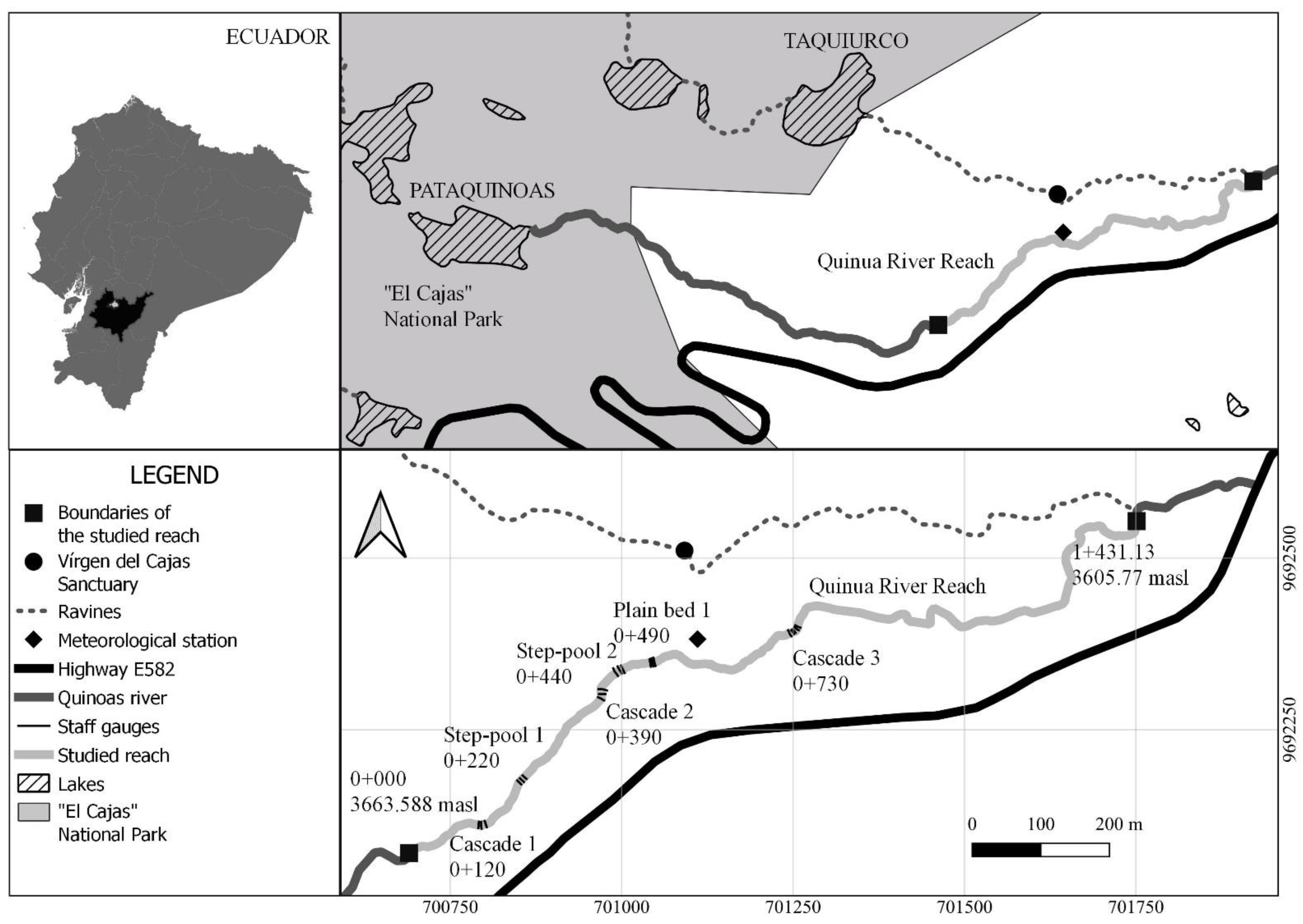
The Quinoas reach, tributary of the Paute river basin, located between the eastern and western cordillera of the Andes in Ecuador, was selected for this study. The reach understudy has a length of 1.5 km and contains different morphologies such as plane-beds, cascades, and step-pools. The terrain level upstream of the reach (0 + 000) is 3664.4 m.a.s.l. and that downstream of the study reach is (1 + 431.13) 3605.77 m.a.s.l., resulting in an average bed slope of 4%. The following morphologies were selected in the 1.5 km river reach: Step-pool 1, Plane-bed 1, and Cascade 3 (see Figure 1 for their location), named herein in this article Step-pool, Plane-bed, and Cascade, respectively.
2.2. Field Data
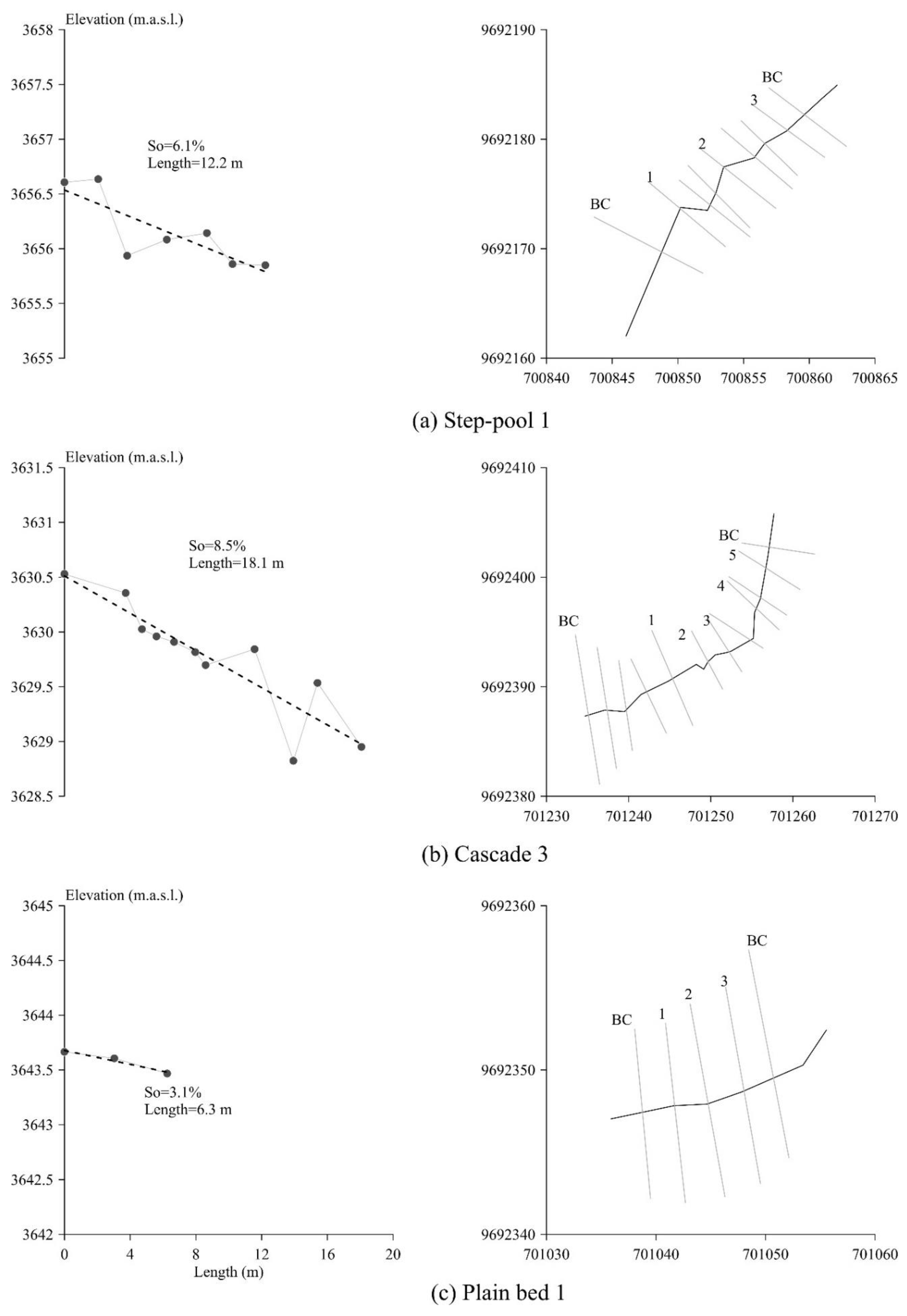
Topographic information was gathered using a differential GPS and total station survey with the objective of capturing critical details with adequate measurement precision (see Figure 2). The measured cross-sections (XSs) were taken at certain locations such as changes in bed slope or changes across XSs.
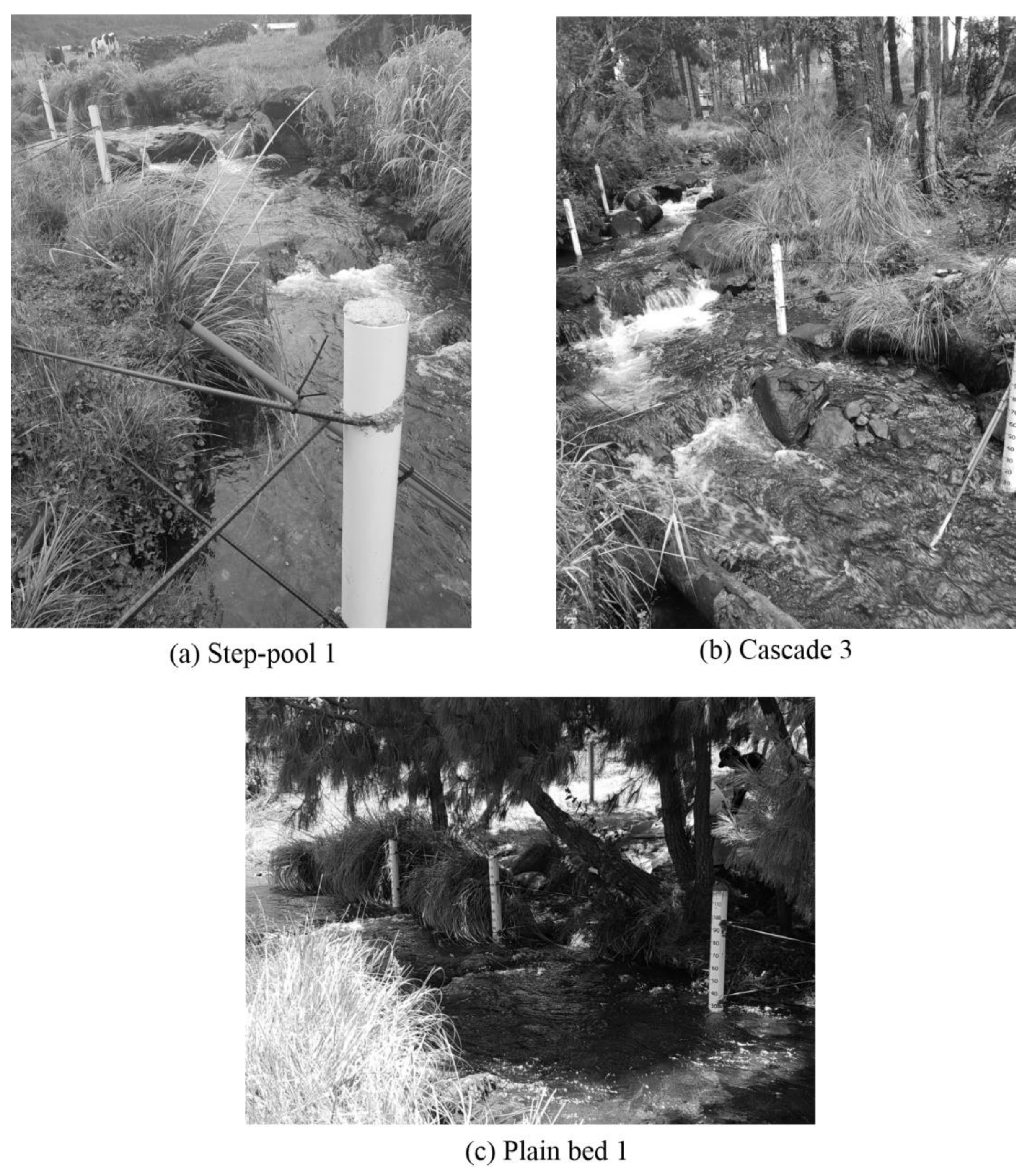
Three staff gauges were used for measuring the water levels in the Step-pool 1 and Plane-bed 1 reaches (Figure 2a,c, respectively) and five staff gauges in the Cascade 3 reach (Figure 2b). In addition, at every staff gauge, the wetted width (w) was measured, while the discharge (Q) was estimated using the dilution-gauging method with salt as a tracer [15]. Figure 3 depicts the studied reaches and the used staff gauges.
The flow velocity (U) was determined using two conductance curves, located upstream and downstream in each reach, using the Harmonic methodology [16] for defining the travel time. The velocity was calculated as the ratio between the distance between staff gauges and the mean travel time. The Friction Slope (SF) was approximated with the water surface slope (Sw) [17], and the bed material distribution size was estimated using the pebble counting approach [18] with a sample of 400 particles. The roughness coefficient was initially determined with the Darcy–Weisbach equation (Equation (1)) with average geometric values for the cross-section of the selected reach. Thereafter, the f coefficient was transformed into Manning’s roughness parameter n using Equation (2).
f = (8 × g × Rh × Sf)/U2
PRP = n = [(f × Rh1/3)/(8 × g)]0.5
2.3. Numerical Scheme
The hydrodynamic model chosen in this research was the 1-D component of HEC-RAS, developed by the Hydrologic Engineering Center (HEC) of the United States Army Corps of Engineers. In this study, all simulations were performed assuming steady-state conditions. The energy equation (Equation (3)) is solved between two adjacent XSs, while, in the case of not obtaining an equilibrium, the numerical algorithm uses the critical depth response given the specific condition. In cases of rapidly varying flow, HEC-RAS solves the momentum equation.
where z is the elevation of the main channel (m), y is the water depth (m), U is the velocity (m s−1), g is the gravity acceleration (m s−2), and he is the energy head loss (m) (Equation (3)). The subscript in XS, 2 and 1, refers to upstream and downstream, respectively.
z2 + y2 + α2 × U22/(2 × g) = z1 + y1 + α1 × U12/(2 × g) + he
The energy head loss (Equation (4)) comprises the loss due to roughness and contraction/expansion losses. Different methodologies are available to estimate the representative friction slope between two cross-sections (RFSM): the average conveyance equation (Equation (5) ACE, the default methodology in HEC-RAS), the average friction slope equation (Equation (6) AFSE), the geometric mean friction slope equation (Equation (7) GMFSE), and the harmonic friction slope equation (Equation (8) HMFSE).
where L is the reach length (m), RFSM is the friction slope between two XSs, and CC is a contraction expansion coefficient. RFSM is calculated using Equation (5).
where Q is the flow rate (m3 s−1) and K is the conveyance (m3 s−1). RFSM can also be calculated using Equations (6)–(8), respectively:
where Sf1 is the friction slope at the upstream XS and Sf2 is the friction slope at the downstream XS.
he = L × RFSM + CC ×|α2 × U22/(2 × g) − α1 × U12/(2 × g)|
RFSM = [(Q1 + Q2)/(K1 + K2)]2
RFSM = (Sf1 + Sf2)/2
RFSM = (Sf1 × Sf2)0.5
RFSM = (2 × Sf1 × Sf2)/(Sf1 + Sf2)
As the velocity distribution of the water flow in a channel presents three-dimensional characteristics, it is necessary to correct it with the coefficients α and β to maintain the energy and momentum flux when the mean cross-section velocity is used [19]. α is obtained with a flow-weighted average in the main channel and overbanks (Equation (9)). Given that the experiments developed in the current research are inbank flow and the water surface is considered as horizontal [5], α will be equal to one.
where Klob, Kmc, and Krob are the conveyance at the left overbank, main channel, and right overbank (m3 s−1), respectively; Kt is the total conveyance (m3 s−1); Alob, Amc, and Arob are the flow areas at the left overbank, main channel, and right overbank (m2), respectively; and At is the total flow area (m2).
α = [At2 × (Klob3/Alob3 + Kmc3/Amc3 + Krob3/Arob3)]/Kt3
For each study reach, the effect of the geometric description was analyzed. The topographic information (Figure 3) was used as a base to include additional XSs interpolated at equidistant distances (one meter, fifty centimeters, and twenty-five centimeters). At each run, the errors and warnings were checked and documented. The final geometric model for each reach was the one without any warning. This test used the physical roughness as the effective roughness for each case. The validation data to verify the performance of each model were the water levels in the staff gauges. These water levels were transformed into water levels relative to the deepest cross-section point. The water depth resulting from the model was transformed in the same way to be compared with the measurements. Ultimately, the HEC-RAS model was run under a steady-state condition with a mixed flow regime (i.e., subcritical and supercritical flow). The boundary conditions in the cross-sections labeled as BC in Figure 2 were normal depth. The validation data consisted of water levels taken from staff gauges labeled with a number in Figure 2.
2.4. The GLUE Methodology
Two GLUE experiments with variable roughness values were performed for three different flows at each reach. Experiment 1 consisted of 5000 runs for each RFSM: ACE (Equation (5)), AFSE (Equation (6)), GMFSE (Equation (7)), and HMFSE (Equation (8)), while in Experiment 2, HEC-RAS internally selected the RFSM (8000 runs) based on profile type and flow regime. The GLUE process was implemented using the HEC-RAS Controller in Visual Basic Excel ® (Microsoft Corporation, Redmond, WA, USA) [20]. The range of roughness coefficients (Manning values) was selected to cover all the possible variations [12] and considering a uniform distribution [5]. The range 0.03–0.5 was imposed using as a criterion for the minimum value recommended in Brunner [21] for mountain streams and for the maximum value measured in the field campaigns. However, the step-pool roughness range needed to be extended up to 0.7 for low flows as the previous roughness range was not wide enough to capture a peak in the likelihood curve. In Experiment 1, each RFSM was identified with a number (1: Equation (5), 2: Equation (6), 3: Equation (7), 4: Equation (8)) and was selected considering a uniform distribution.
There is no universal likelihood function for GLUE experiments [6]; indeed, Jung and Merwade [13] found that different likelihood functions produced different uncertainty bounds (5–95%) that did not produce important changes in the overall uncertainty quantification of an inundation map. In this research, the likelihood function included the sum of root-mean-square error (RMSE), mean average error (MAE), and the standard deviation of residuals (SDR). These metrics were normalized by applying Equation (10). RMSE and MAE represent the residuals’ mean having different weights in the average procedure, while SDR is a dispersion of the residuals measure. The likelihood value is one when the measurements exactly coincide with the modeling result.
where Om is the observations’ mean.
Likelihood = 1 − RMSE/Om − MAE/Om − MSDR/Om
2.5. Uncertainty Measurement Analysis PRP
The uncertainty of direct measurements such as wet width (w) and water level (η) were determined by repeating measurements. Resolution and random errors were combined in the measurements (Equation (11)).
where δX is the absolute uncertainty of X and XO is the central value of the variable.
Relative Uncertainty (%) = δX/ δXO
The uncertainty of indirect measurements (W in Equation (12)), which was estimated based on direct measurements of X, Y, and Z, is given by Equation (12) [22]. The result of Equation (12) was used to obtain the range of variations in W with Equation (13).
where δW is the absolute uncertainty of W, WO is the central value of the variable, and W is the range of possible values of this variable.
δW = | ∂Q/∂X |O δX+| ∂Q/∂Y |O δY +| ∂Q/∂Z |O δZ
W = WO +/− δW
3. Results
3.1. Likelihood Curves
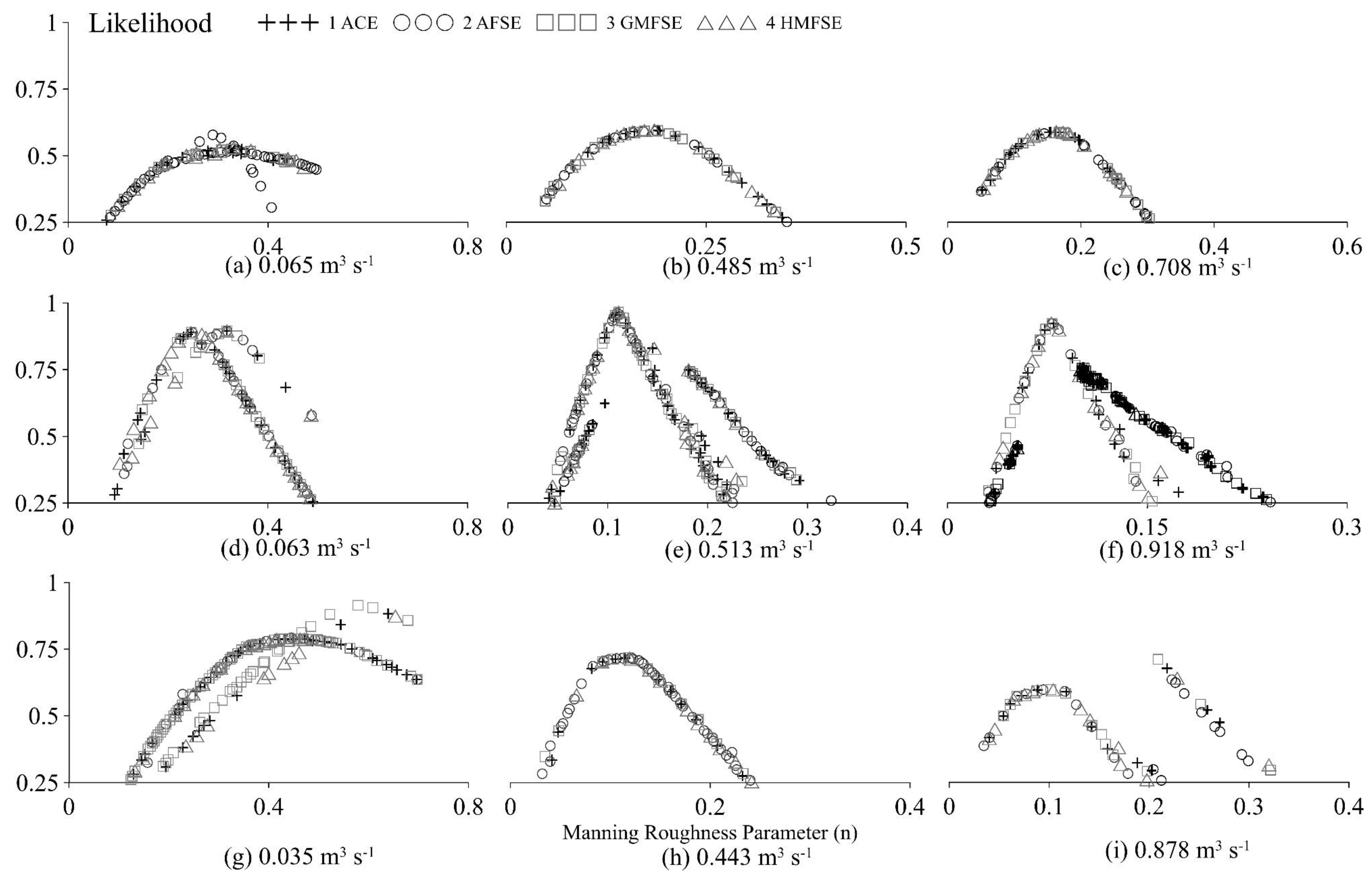
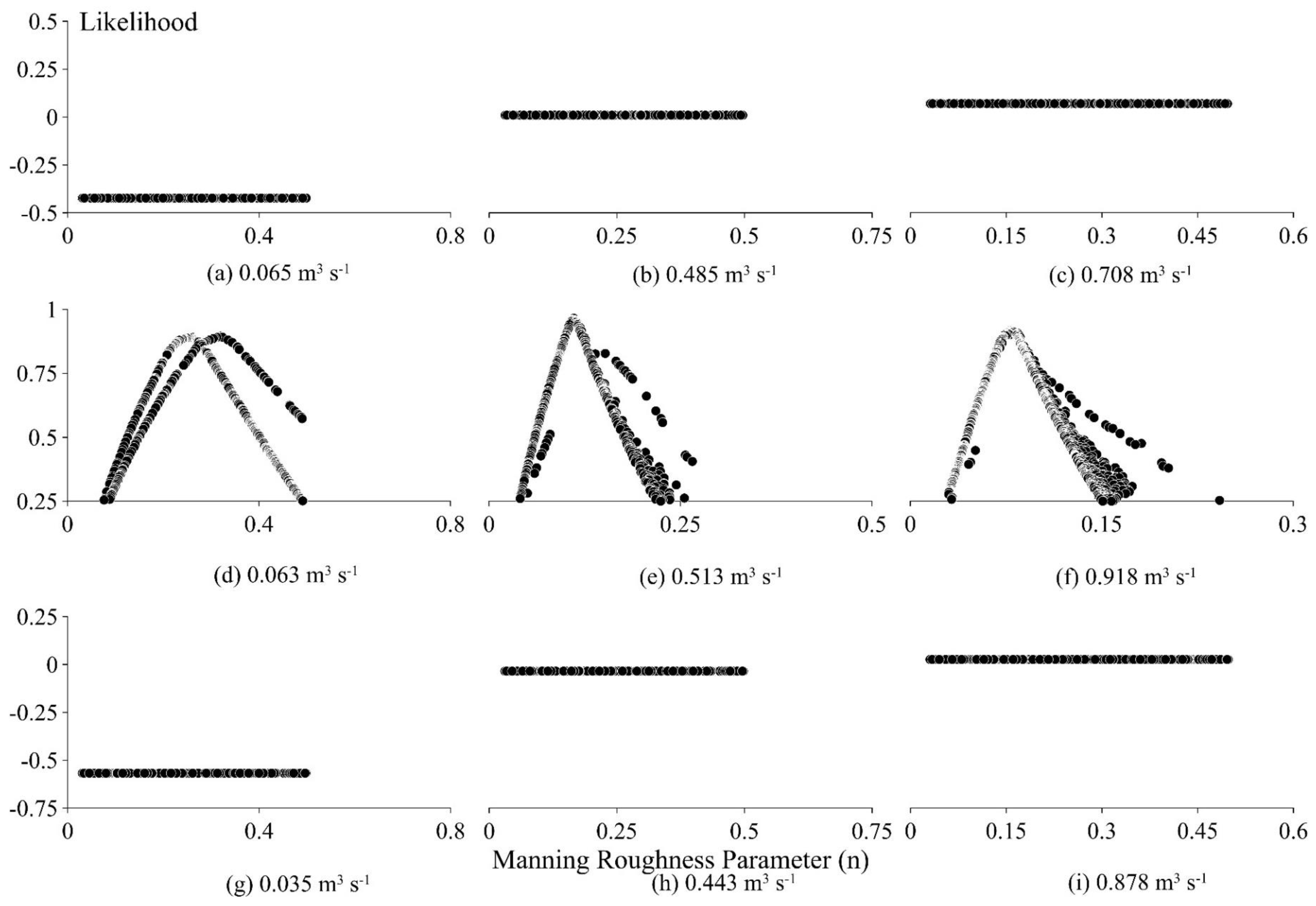
The results of the first GLUE experiment in which the roughness coefficient in the three morphologies was varied according to each RFSM method are presented in Figure 4.
For practical purposes, only the points with a probability threshold greater than 0.25 are shown as lower values are considered as nonbehavioral by not providing relevant information.
Figure 4 reveals that the resulting likelihood curves are concave downward with one or two peaks depending on the flow magnitude and morphology. Cascade has two slightly different likelihood peaks for low flow, but for mid and high flows, there is only one performance peak. Plane-bed has two performance peaks for all flow magnitudes. Step-pool at low flow has two peaks, while at high flow, there is one peak in a concave downward curve in the left and one maximum in a linear pattern in the right. For mid flow, there is a single likelihood peak.
Figure 4a presents the formation of two likelihood curves; the higher performance curve has points from AFSE exclusively, while the lower performance curve is composed of points from all RFSMs. Figure 4d–f show the formation of two likelihood curves composed from all RFSM points. In the cases under study, the one in Figure 4g presents the formation of two likelihood curves, where it can be observed that the one with the best performance is composed only of the GMFSE points. Special attention should be given to the likelihood curves in Figure 4i, where the formation of a curve without concavity can be observed on the right side of the figure. Those results are further discussed in the Discussion section in the subsection Likelihood Curves. Cascade peaks have the lowest performance values (~0.6) in all cases under analysis (Figure 4a–c). Plane-bed has peak performance values greater than 0.89 (Figure 4d–f), while step-pool peak performance values decrease with flow magnitude, ranging from 0.91 to 0.61 (Figure 4 g–i).
The results of the second GLUE experiment (8000 runs) in which HEC-RAS selects RFSM are depicted in Figure 5. Step-pool and cascade show a linear horizontal likelihood trend (constant) with low-performance values. Plane-bed likelihood curves are presented in Figure 5d–f. The shapes of the curves present concavity downward with peak performance values greater than 0.89.
3.2. Field Mesurements Uncertainty
Uncertainties in the direct measurement used to estimate the resistance parameter are the wetted width, water level, velocity, and flow. The wetted width uncertainty is less than 0.14% of the standard uncertainty, while water level (η) has a 1.5% of standard uncertainty; these values are comparable to those found by Lee and Ferguson [23]. The uncertainties for velocity and flow measurement were taken from Lee and Ferguson [23] as 5% as tracers were used for the flow and the centroid method for the velocity calculation. The indirect measurement uncertainties are 10% for the water depth, comparable with the 12% obtained by Lee and Ferguson [23], 10% for the hydraulic radius, 17% for the energy slope, and 19% for (8/f)1/2. The former value is comparable with 17% for (1/f)1/2 found by Lee and Ferguson [23]. Based on the above information, the Manning roughness parameter (n) uncertainty was estimated at 22% of the standard deviation.
3.3. Effective and Measured Roughness Values
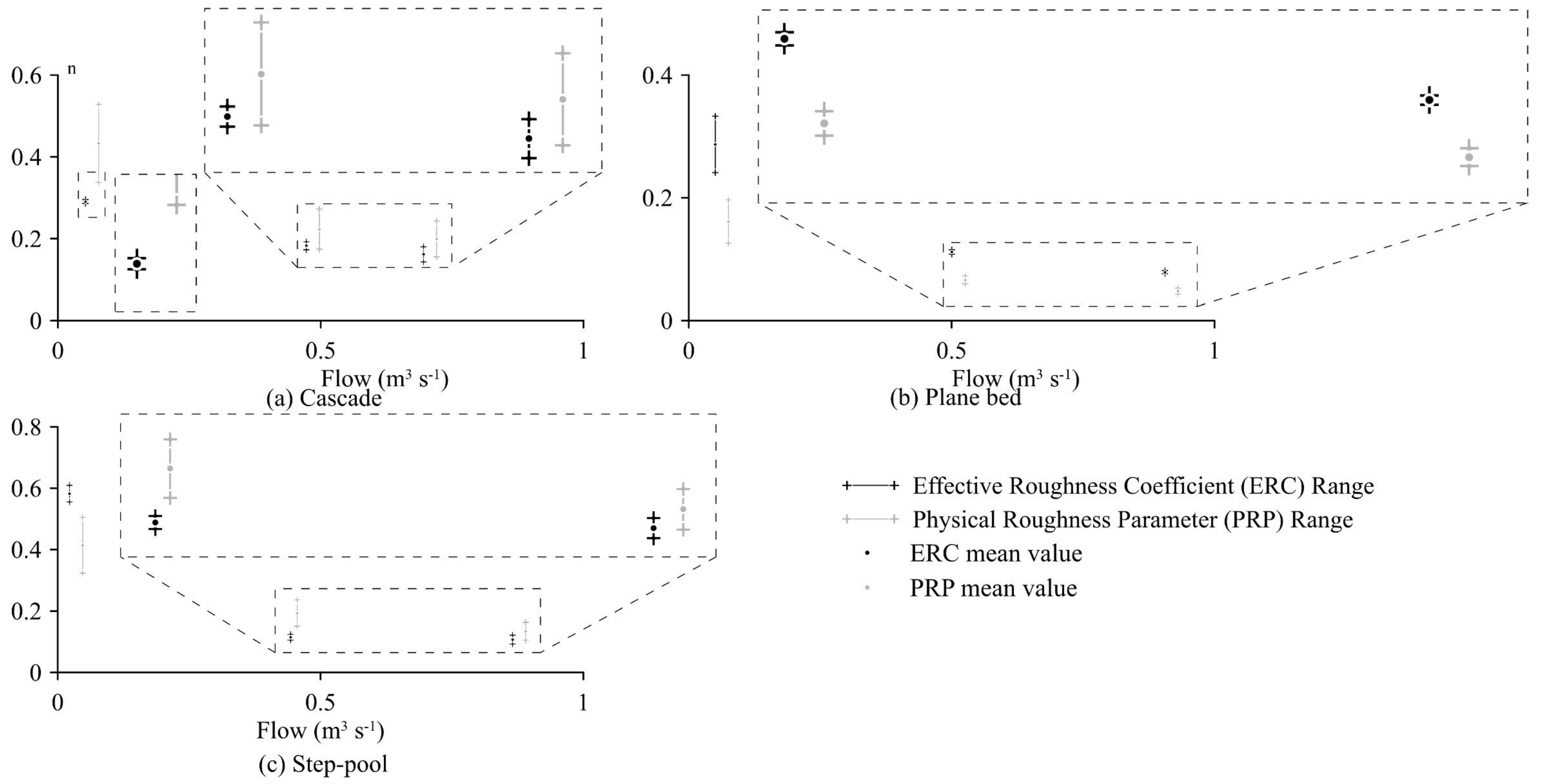
The value ranges of the effective roughness coefficient (ERC)—calibrated—and physical roughness parameter (PRP)—measured—for different flow rates in Experiment 1 (changing roughness and RFSM at the same time) are shown in Table 1 and Figure 6. The range of ERC values was obtained from the analysis of the maximum likelihood curves (Figure 4), while the range of PRP values was the result of the indirect n measurement and the uncertainty analysis. Table 1 compares the PRP, velocity, and Froude numbers measured in this study with those in the literature [24,25].
The comparison in Table 1 shows that the values of the data calculated in the present study are among the measured ranges presented in the literature. An important aspect to emphasize is that the Froude number presents a value lower than that in all the sections studied despite the steep slopes. Jarret [26] stated that extreme turbulence, energy loss produced by the channel, cross-sectional variations, and interactions of the water with the boulders increase the resistance to flow. Jarret [26] noted localized areas of supercritical flow, for example, in areas where the flow passes over large clasts. In Figure 3, the same pattern can be noticed, in which, in certain areas, supercritical flow is presented.
The difference between the ranges of ERC and PRP decreases with the magnitude of flow (seen from a quantitative and qualitative point of view according to Table 1 and Figure 6, respectively). The range values in ERC and PRP overlap for medium and high flows in cascade, while in plane-bed, the range values do not. In step-pool, the range values in ERC and PRP intersect only at high flow rates. Table 2 illustrates the results of Experiment 2 where the RFSM values are selected by HEC-RAS. Cascade and step-pool GLUE experiments did not provide a valid response, as for all roughness values tested, there is equifinality with a low likelihood (below the threshold value).
The low flow ERC range for plane-bed, listed in Table 1, is higher than the interval stated on Table 2. The values of both experiments coincide in the lower limit while they differ in the upper limit, in which the value of experiment 1 is higher. The values for the remaining flow magnitudes are the same for both experiments. Given that the results of cascade and step-pool in Table 2 cannot be used, and the results of plane-bed differ between both experiments only at low flows without improving the peak likelihood, the comparison of ERC and PRP is based on the information in Table 1 in Section 4: Discussion.
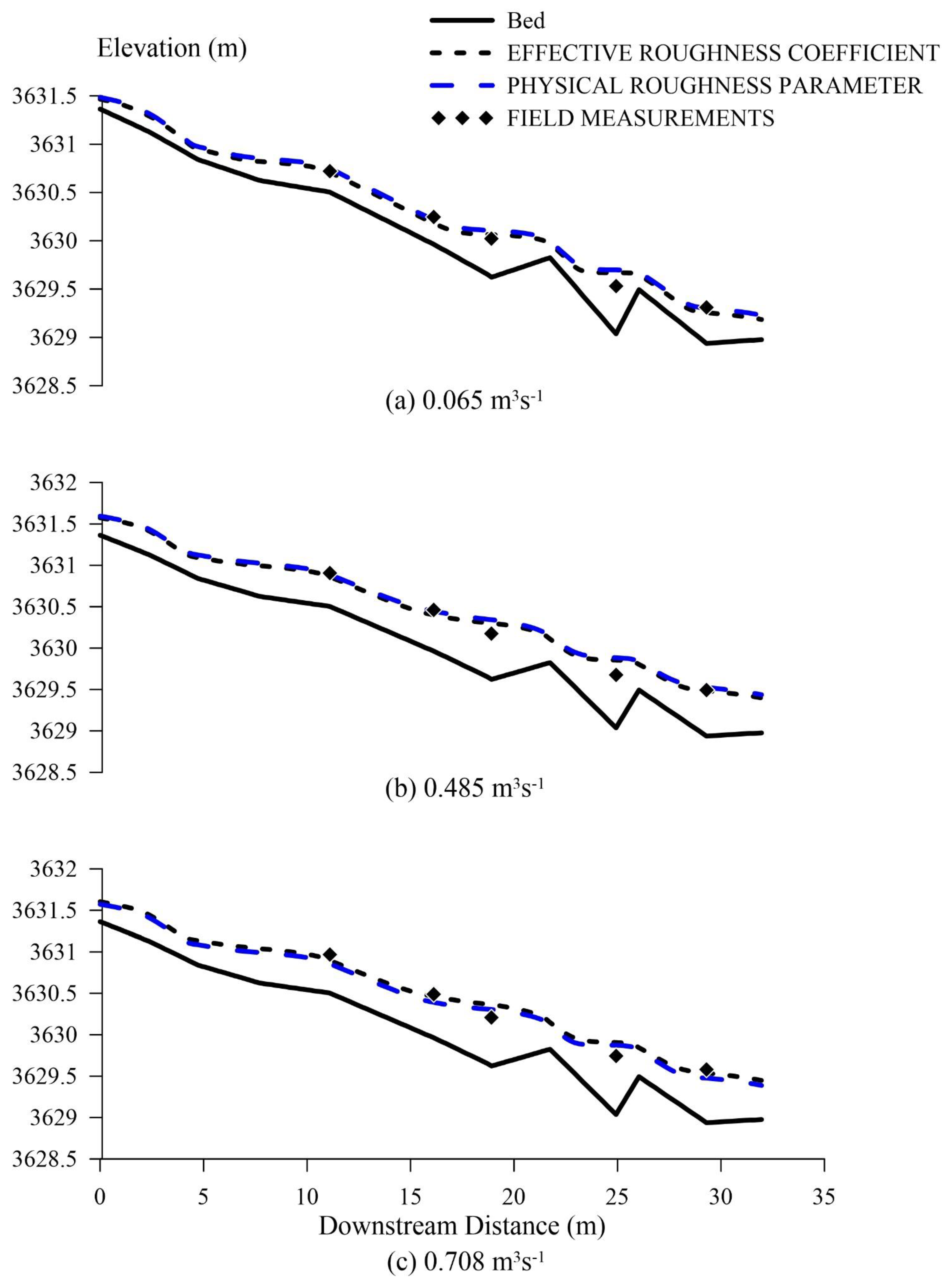
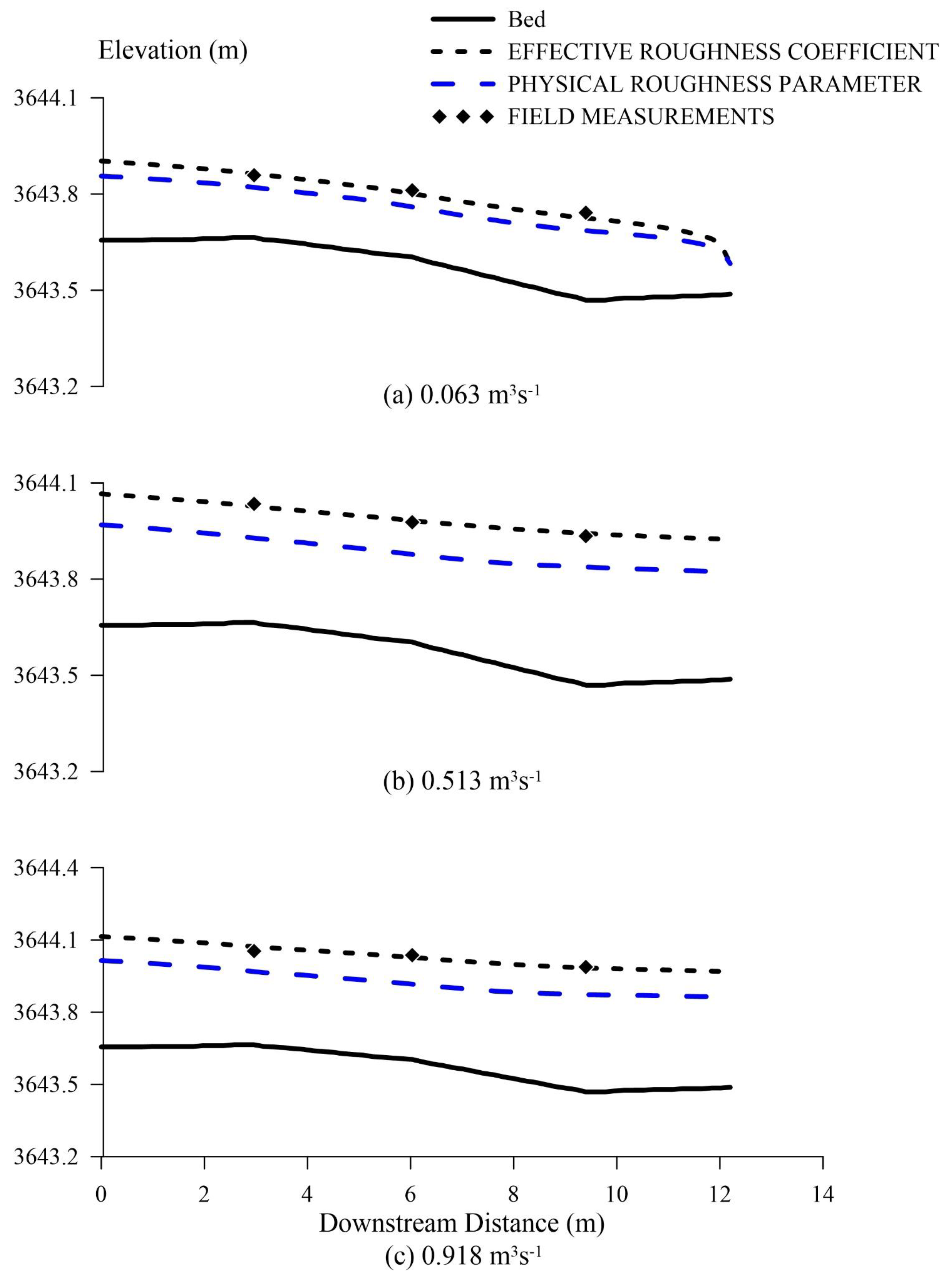
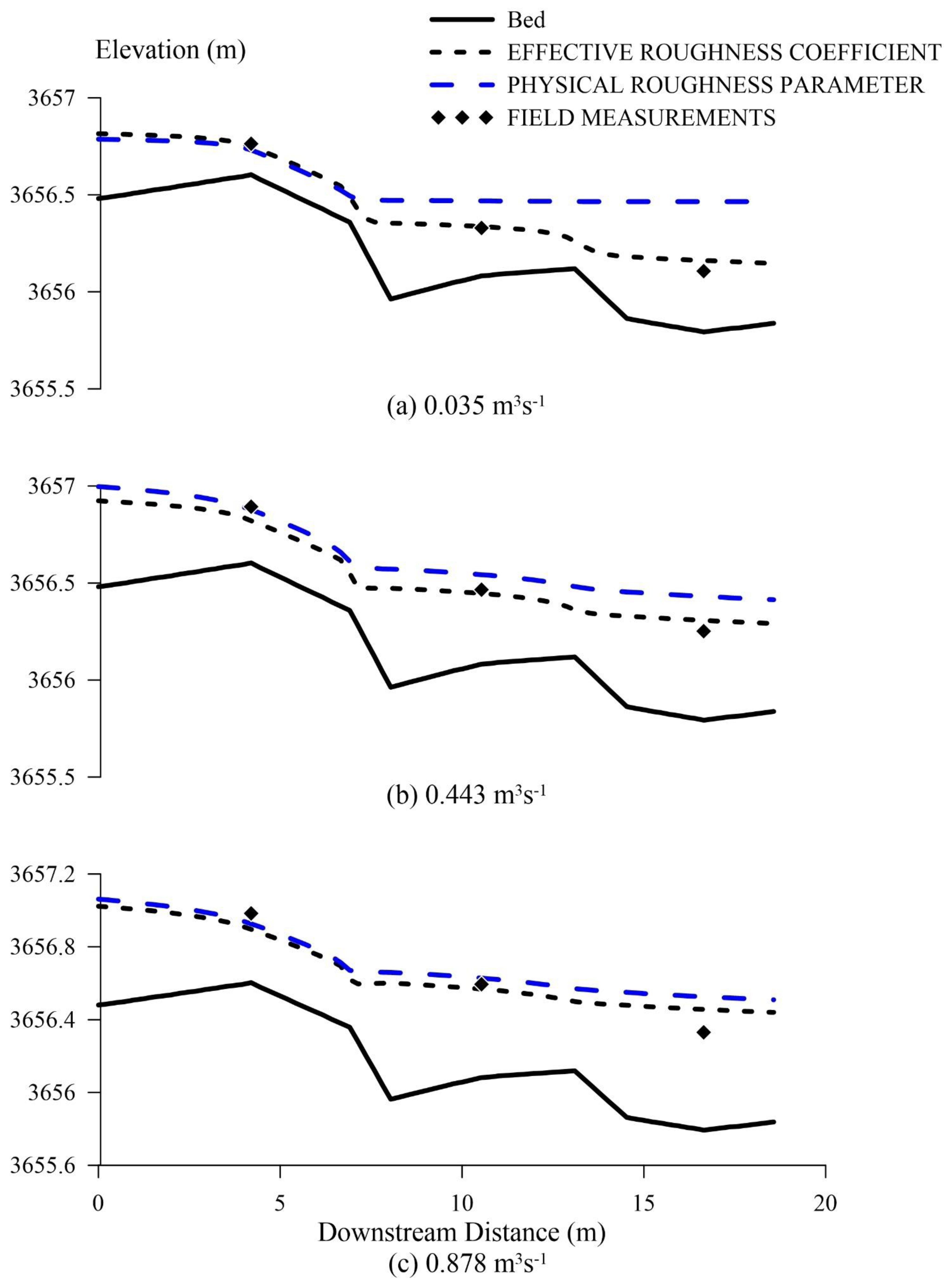
Figure 7, Figure 8 and Figure 9 depict the field-measured water depths, as well as the water surface profile obtained with ERC and PRP (Refer to Table 1). Cascade water depth profiles show that the field data at 24.93 m can be predicted by neither of the parameters, resulting in a low likelihood value obtained for this morphology. Nevertheless, the use of ERC in the model results in a better prediction of points at 18.91 and 24.93 m at low flow. Moreover, for mid and high flow, the intersection of ERC and PRP values makes sense as there is no marked difference between both water surface profiles. Figure 8 shows a notable difference in the water surface profile between both roughness parameters in plane-bed.
ERC considerably increases the predictive capacity of the model, which means that it does not cross with PRP. Besides, all the field measurements are closely predicted when using ERC, resulting in the high likelihood values previously mentioned. Figure 9 illustrates that the use of ERC in step-pool improves the model predictability at low and mid flow, but at high flow, both parameters produce a similar water surface profile. This aspect justifies the intersection of ERC and PRP only at high flows. The descending likelihood value in step-pool is because of the descending prediction capacity to predict the field measurement at 4.2 m.
4. Discussion
4.1. Likelihood Curves
Figure 4 shows that plane-bed for all flows (Figure 4d–f) and step-pool for high flows (Figure 4i) have two likelihood curves. The right-sided likelihood curve in plane-bed is formed when, in the solution, the HEC-RAS numerical model presents the critical depths as a response. This response occurs when, in the iterative process of solving the energy equation, a solution is not found under a specified tolerance given a maximum number of iterations. Note that a critical depth response is not expected in this morphology. Likewise, the curve on the right side in step-pool is formed by the critical depths as responses from the numerical model. The shape of this likelihood curve does not allow a maximum value to be obtained, and it is ignored for analysis.
4.2. Likelihood Peak Values
In the 1-D numerical approach, horizontal water levels in the XS are assumed [21]; however, this assumption deviates from reality at certain morphologies in the headwater of mountain rivers.
The bed of cascade has randomly distributed large clasts consisting of alluvial boulders and cobbles [27]. The water interaction with boulders or cobbles produces both a jet flow and a wake flow around the particles, forming eddy currents behind obstacles, whereas the flow above the described particles produces a tumbling flow [26,27]. The physical process described contrasts with the measured water level at a single point near the bank, resulting in low performance in the outputs of the numerical model, and thus in low peak likelihood values for all flow magnitudes (~0.6 according to Table 1).
Plane-bed flow is closer to the 1-D numerical model assumptions as there are no bedforms, there is no tumbling flow, and the bed material is smaller [27], leading to the representative water level measurement of the XS and the high peak likelihood values (~0.9 according to Table 1).
Step-pool presents a staircase shape (where risers are steps and pools are treads) with a tumbling flow pattern [28]. Water levels are measured in pools. At low flow, the effect of water plunging into pools does not produce a significant free-surface variation, while, as the flow increases, there is an appreciable free-surface variation. This causes the horizontal water level assumption to be invalid. This is the explanation behind the decline in the likelihood peak starting with a value of 0.9 at low flow and decreasing to 0.6 for high flow.
4.3. Friction Slope Methodology
Two studies were found in the literature investigating the influence of RFSM on the model performance when the energy equation is used. Laurenson [29] tested different RFSM performances using analytical data. The validation data consisted of water levels from a cubic equation. According to this analysis, AFSE is the best and safest methodology to predict water levels. Artichowicz and Mikos-Studnicka [30] tested four theoretical cases in a prismatic channel (three tranquil flows and one rapid flow) using the solution of the differential energy equation as validation data. In this study, the analyzed RFSM included all the methodologies available in HEC-RAS and some additional methods available in the literature. AFSE was the best methodology for tranquil flow; on the other hand, HMFSE was the best methodology for rapid flow. There are important differences between previous studies and the current study. First, the selection of the RFSM methodology does not influence most of the GLUE results except for cascades and step-pools at low flows (see Table 1). The cascade reach in this research could be considered similar to the rapid flow case in Artichowicz and Mikos-Studnicka [30]. However, in our study, the best RFSM for cascade at low flow was AFSE (Equation (6)), unlike the HMFSE (Equation (8)) obtained by Artichowicz and Mikos-Studnicka [30]. A possible explanation for this difference might be that the Artichowicz and Mikos-Studnicka [30] test is performed in a prismatic flume without bed material, while cascade has boulders and cobbles interacting with the flow. Furthermore, the cascade results agree with Laurenson [29] who advised AFSE. A case similar to step-pool could not be found in the literature. The best-performing RFSM for low flow was GMFSE (Equation (7)). The authors believe that GMFSE is superior due to its resilience to outliers [31]; in this morphology, it is important that tumbling flow produces abrupt changes in the friction slope. In addition, neither Artichowicz and Mikos-Studnicka [30] nor Laurenson [29] had, in their study, big particles in the riverbed as in our case.
HEC-RAS chose RFSM (Experiment 2) based on both the profile type when it is subcritical or supercritical and the magnitude of the friction slope of the previous XS [21]. However, it seems that high slopes, large-scale roughness elements, slope breaks, or tumbling flow produce the same water levels for any roughness when this option is chosen, thus losing physical realism. Nevertheless, the use of this option in the plane-bed produced the same results as using any other of the four available methodologies. This could mean that the automatic selection of RFSM could be conditioned to lowland rivers.
4.4. Effective Roughness Coefficient (ERC) and Physical Roughness Parameter (PRP)
Several GLUE studies on cascade, plane-bed, and step-pool were not found, as indicated by the relatively low number of references in the Introduction section; therefore, it is not possible to compare the likelihood curves with other references. Moreover, none of the studies found in the literature made a comparison between effective and measured roughness values.
ERC contains the same energy dissipation process as PRP [11,32], but 3-D effects and geometry errors are not represented in the used 1-D model. Furthermore, in this study, the effect of inaccuracies in geometry is minimal due to the high precision of the used measuring equipment (total station and differential GPS), and the consideration of strategic points (slope changes, before and after steps) was considered in the studied reaches to obtain data.
The parameter α in the energy equation (Equation (3)) must be considered when comparing ERC and PRP. Α assumes a value equal to 1 because there is inbank flow only (see Equation (9)), so there is no correction, due to the three-dimensional characteristic of the flow.
4.4.1. Low Flow
For low flow rates in plane-bed and steep-pool morphologies, the range of ERC values is above the range of PRP values (Figure 6b,c, respectively), contrary to what is presented in cascade (Figure 6a). Through linear interpolation of the data in Table 3, it was found that, on average, 40% of the bed material in all morphologies under study protrudes above the water level at low flow flows, having an important influence on resistance. In cascade, the water level shows an alteration due to the interaction of the water with the large clasts [17]. A lower value of ERC with respect to PRP could mean that the numerical model requires the increase in velocity to account for the jetting flow effect around boulders and cobbles [27]. Plane-bed and step-pool depict a similar pattern when comparing ERC with PRP. The water surface variation is significantly lower in plane-bed than cascade because there are fewer boulders and cobbles (see Table 3), and the flow velocity is lower, so the resistance is smaller. At step-pool, there is flow division at steps, so water plunges into the pool at multiple points, reducing the water surface variation. The higher ERC relative to PRP in plane-bed and step-pool may be due to the need of the model for a lower velocity.
4.4.2. Mid to High Flow
According to Figure 6, the different pattern between ERC and PRP was preserved except for step-pool having the same pattern as cascade rather than the previous plane-bed pattern. In step-pool, as the flow increases, both ranges approach each other and overlap for the highest flow tested. The changing difference between ERC and PRP in step-pool may be attributed to a higher water surface deformation during tumbling flow. A higher flow leads to less flow division at steps, so there is a concentrated amount of water plunging into the pool. In cascade (Figure 6a), the bounds of ERC and PRP intersect for mid and high flow, but in plane-bed (Figure 6b), both ranges do not overlap. The possible reason could be the presence of vegetation near the main channel in plane-bed as can be observed in Figure 3c. At mid and high flows, the leaves of the vegetation interact with water, increasing flow resistance. This phenomenon cannot be represented in the model, so ERC may need to be modified to account for it.
5. Conclusions
The difference between the effective (ERC) and physical (PRP) roughness values of three typical morphologies found in mountain rivers (cascade, plane-bed, and step-pool) was analyzed. River flow, mean velocity, topographic data, water levels, and wetted width were monitored, and the measured roughness was estimated based on the average of the cross-sectional data. An effective value of the roughness parameter was derived in two GLUE experiments using the HEC-RAS controller to automate the simulations. The comparison between effective and physical roughness was limited to three flow magnitudes: low, mid, and high, because of the computational power required for the GLUE experiments and the available field data. The likelihood function was a combination of two measures of the mean residual and one measure of the standard deviation of residuals.
The research yielded two important findings. First, the RFSM influence (Experiment 1) on hydrodynamic models was limited to low flows. The results of the step-pool model were the most affected when different methodologies were used, and as a result, four different likelihood curves were found. When HEC-RAS selected the RFSM (Experiment 2) only for plane-bed, acceptable results were found. In cascade and step-pool, equifinal values were obtained for all roughness values, losing physical significance. Second, the highest difference between ERC and PRP was at low flows. As the flow increased, the difference between ERC and PRP ranges decreased and, in some cases, even overlapped. Cascade and plane-bed had opposing patterns when ERC was compared with PRP bounds, while step-pool ERC and PRP patterns depended on the flow magnitude. ERC is a key element in a hydrodynamic model, so a careful selection of the ERC value must be pursued considering morphologies and flow data. Future research could include a wider range of flow magnitudes to compare the different tendencies between effective and physical roughness values.
Author Contributions
Conceptualization, S.C. and E.S.-C.; methodology, S.C. and E.S.-C.; software, S.C.; validation, S.C., E.S.-C. and L.T.; formal analysis, S.C. and E.S.-C.; investigation, S.C.; resources, A.A.; data curation, S.C.; writing—original draft preparation, S.C.; writing—review and editing, S.C., E.S.-C., L.T., E.S. and A.A.; visualization, S.C.; supervision, A.A. and E.S.-C.; project administration, E.S. and A.A.; funding acquisition, A.A. All authors have read and agreed to the published version of the manuscript.
Funding
This research was funded by the Research Directorate of the University of Cuenca and developed within the framework of the project “Towards a sound mathematical description of the dispersion of pollutants in mountain rivers”.
Institutional Review Board Statement
Not applicable.
Informed Consent Statement
Not applicable.
Data Availability Statement
The data presented in this study are available on request from the corresponding author. The data are not publicly available, due to a confidentiality agreement of the financing project “Towards a sound mathematical description of the dispersion of pollutants in mountain rivers”.
Acknowledgments
The authors are thankful to Jan Feyen for reading the manuscript. This manuscript is an outcome of the Doctoral Program in Water Resources by the first author, jointly offered by Universidad de Cuenca, Escuela Politécnica Nacional, and Universidad Técnica Particular de Loja.
Conflicts of Interest
The authors declare no conflict of interest.
References
- Morvan, H.; Knight, D.; Wright, N.; Tang, X.; Crossley, A. The concept of roughness in fluvial hydraulics and its formulation in 1D, 2D and 3D numerical simulation models. J. Hydraul. Res. 2008, 46, 191–208. [Google Scholar] [CrossRef]
- Cook, A.; Merwade, V. Effect of topographic data, geometric configuration and modeling approach on flood inundation mapping. J. Hydrol. 2009, 377, 131–142. [Google Scholar] [CrossRef]
- Teng, J.; Jakeman, A.J.; Vaze, J.; Croke, B.F.W.; Dutta, D.; Kim, S. Flood inundation modelling: A review of methods, recent advances and uncertainty analysis. Environ. Model. Softw. 2017, 90, 201–216. [Google Scholar] [CrossRef]
- Papaioannou, G.; Vasiliades, L.; Loukas, A.; Aronica, G.T. Probabilistic flood inundation mapping at ungauged streams due to roughness coefficient uncertainty in hydraulic modelling. Adv. Geosci. 2017, 44, 23–34. [Google Scholar] [CrossRef] [Green Version]
- Pappenberger, F.; Beven, K.; Horritt, M.; Blazkova, S. Uncertainty in the calibration of effective roughness parameters in HEC-RAS using inundation and downstream level observations. J. Hydrol. 2005, 302, 46–69. [Google Scholar] [CrossRef]
- Blasone, R.S.; Vrugt, J.A.; Madsen, H.; Rosbjerg, D.; Robinson, B.A.; Zyvoloski, G.A. Generalized likelihood uncertainty estimation (GLUE) using adaptive Markov Chain Monte Carlo sampling. Adv. Water Resour. 2008, 31, 630–648. [Google Scholar] [CrossRef] [Green Version]
- Aronica, G.; Bates, P.D.; Horritt, M.S. Assessing the uncertainty in distributed model predictions using observed binary pattern information within GLUE. Hydrol. Process. 2002, 16, 2001–2016. [Google Scholar] [CrossRef]
- Bozzi, S.; Passoni, G.; Bernardara, P.; Goutal, N.; Arnaud, A. Roughness and Discharge Uncertainty in 1D Water Level Calculations. Environ. Model. Assess. 2015, 20, 343–353. [Google Scholar] [CrossRef]
- Beven, K.; Binley, A. GLUE: 20 years on. Hydrol. Process. 2014, 28, 5897–5918. [Google Scholar] [CrossRef] [Green Version]
- Beven, K.; Binley, A. The future of distributed models: Model calibration and uncertainty prediction. Hydrol. Process. 1992, 6, 279–298. [Google Scholar] [CrossRef]
- Bhola, P.K.; Leandro, J.; Disse, M. Reducing uncertainty bounds of two-dimensional hydrodynamic model output by constraining model roughness. Nat. Hazards Earth Syst. Sci. 2019, 19, 1445–1457. [Google Scholar] [CrossRef] [Green Version]
- Aronica, G.; Hankin, B.; Beven, K. Uncertainty and equifinality in calibrating distributed roughness coefficients in a flood propagation model with limited data. Adv. Water Resour. 1998, 22, 349–365. [Google Scholar] [CrossRef]
- Jung, Y.; Merwade, V. Uncertainty quantification in flood inundation mapping using generalized likelihood uncertainty estimate and sensitivity analysis. J. Hydrol. Eng. 2012, 17, 507–520. [Google Scholar] [CrossRef]
- Horritt, M.S.; Bates, P.D. Evaluation of 1D and 2D numerical models for predicting river flood inundation. J. Hydrol. 2002, 268, 87–99. [Google Scholar] [CrossRef]
- Hudson, R.; Fraser, J. Introduction to salt dilution gauging for streamflow measurement, Part IV: The mass balance (or dry injection) method. Streamline Watershed Manag. Bull. 2005, 9, 6–12. [Google Scholar]
- Nitsche, M.; Rickenmann, D.; Kirchner, J.W.; Turowski, J.M.; Badoux, A. Macroroughness and variations in reach-averaged flow resistance in steep mountain streams. Water Resour. Res. 2012, 48. [Google Scholar] [CrossRef] [Green Version]
- David, G.C.L.; Wohl, E.; Yochum, S.E.; Bledsoe, B.P. Controls on spatial variations in flow resistance along steep mountain streams. Water Resour. Res. 2010, 46. [Google Scholar] [CrossRef] [Green Version]
- Bunte, K.; Abt, S.R. Sampling Surface and Subsurface Particle-Size Distributions in Wadable Gravel- and Cobble-Bed Streams for Analyses in Sediment Transport, Hydraulics, and Streambed Monitoring; US Department of Agriculture; Forest Service; Rocky Mountain Research Station: Fort Collins, CO, USA, 2001. [Google Scholar]
- Knight, D.W.; McGahey, C.; Lamb, R.; Samuels, P. Practical Channel Hydraulics: Roughness, Conveyance and Afflux; CRC Press/Taylor & Francis: New York, NY, USA, 2009; ISBN 9780203864180. [Google Scholar]
- Goodell, C. Breaking the HEC-RAS Code: A User’s Guide to Automating HEC-RAS; h2ls: Portland, OR, USA, 2014. [Google Scholar]
- Brunner, G. HEC RAS, River Analysis System Hydraulic Reference Manual; Hydrologic Engineering Center: Davis, CA, USA, 2016. [Google Scholar]
- Fornasini, P. The Uncertainty in Physical Measurements: An Introduction to Data Analysis in the Physics Laboratory; Springer: New York, NY, USA, 2008; ISBN 9780387786506. [Google Scholar]
- Lee, A.J.; Ferguson, R.I. Velocity and flow resistance in step-pool streams. Geomorphology 2002, 46, 59–71. [Google Scholar] [CrossRef]
- Bathurst, J.C. Flow Resistance Estimation in Mountain Rivers. J. Hydraul. Eng. 1985, 111, 625–643. [Google Scholar] [CrossRef]
- Yochum, S.E.; Comiti, F.; Wohl, E.; David, G.C.L.; Mao, L. Photographic Guidance for Selecting Flow Resistance Coefficients in High-Gradient Channels; U.S. Department of Agriculture, Forest Service, Rocky Mountain Research Station: Fort Collins, CO, USA, 2014; Volume 323. [Google Scholar]
- Jarrett, R.D. Hydraulics of high-gradient streams. J. Hydraul. Eng. 1984, 110, 1519–1539. [Google Scholar] [CrossRef]
- Montgomery, D.R.; Buffington, J.M. Channel-reach morphology in mountain drainage basins. Geol. Soc. Am. Bull. 1997, 109, 596–611. [Google Scholar] [CrossRef]
- Chin, A.; Wohl, E. Toward a theory for step pools in stream channels. Prog. Phys. Geogr. 2005, 29, 265–296. [Google Scholar] [CrossRef]
- Laurenson, E.M. Friction Slope Averaging in Backwater Calculations. J. Hydraul. Eng. 1986, 112, 1151–1163. [Google Scholar] [CrossRef]
- Artichowicz, W.; Mikos-Studnicka, P. Comparison of average energy slope estimation formulas for one-dimensional steady gradually varied flow. Arch. Hydroengineering Environ. Mech. 2014, 61, 89–109. [Google Scholar] [CrossRef] [Green Version]
- Dodge, Y. The Concise Encyclopedia of Statistics; Springer Science & Business Media: New York, NY, USA, 2008. [Google Scholar]
- Wohl, E. Mountain Rivers Revisited; John Wiley & Sons American Geophysical Union: Washington, DC, USA, 2013; ISBN 9781118665572. [Google Scholar]
Figure 1.
Location of the 1.5 km river reach with indication of the different morphologies.

Figure 2.
Profiles and topographic characteristics of morphologies under study. (a) Step-pool 1 (b) Cascade 3 (c) Plain bed 1.
Figure 2.
Profiles and topographic characteristics of morphologies under study. (a) Step-pool 1 (b) Cascade 3 (c) Plain bed 1.

Figure 3.
Pictures of analyzed reaches. (a) Step-pool 1 (b) Cascade 3 (c) Plain bed 1.

Figure 4.
GLUE likelihood curves in Experiment 1: Cascade (a–c), Plane-bed (d–f), and Step-pool (g–i).
Figure 4.
GLUE likelihood curves in Experiment 1: Cascade (a–c), Plane-bed (d–f), and Step-pool (g–i).

Figure 5.
GLUE likelihood curves in Experiment 2: Cascade (a–c), Plane-bed (d–f), and Step-pool (g–i).
Figure 5.
GLUE likelihood curves in Experiment 2: Cascade (a–c), Plane-bed (d–f), and Step-pool (g–i).

Figure 6.
Comparison of measured and calibrated n values. (a) Cascade; (b) Plane bed; (c) Step-pool.
Figure 6.
Comparison of measured and calibrated n values. (a) Cascade; (b) Plane bed; (c) Step-pool.

Figure 7.
Water surface profiles using ERC and PRP in Cascade. (a) 0.065 m3s−1 (b) 0.485 m3s−1 (c) 0.708 m3s−1.
Figure 7.
Water surface profiles using ERC and PRP in Cascade. (a) 0.065 m3s−1 (b) 0.485 m3s−1 (c) 0.708 m3s−1.

Figure 8.
Water surface profiles using ERC and PRP in Plane-Bed. (a) 0.063 m3s−1 (b) 0.513 m3s−1 (c) 0.918 m3s−1.
Figure 8.
Water surface profiles using ERC and PRP in Plane-Bed. (a) 0.063 m3s−1 (b) 0.513 m3s−1 (c) 0.918 m3s−1.

Figure 9.
Water surface profiles using ERC and PRP in Step-pool. (a) 0.035 m3s−1 (b) 0.443 m3s−1 (c) 0.878 m3s−1.
Figure 9.
Water surface profiles using ERC and PRP in Step-pool. (a) 0.035 m3s−1 (b) 0.443 m3s−1 (c) 0.878 m3s−1.


Table 1.
Range of values for measured and calibrated n value for Experiment 1.
| Effective Roughness Coefficient (ERC) | Physical Roughness Parameter (PRP) | |||||||||||
|---|---|---|---|---|---|---|---|---|---|---|---|---|
| Site | Flow (m3 s−1) | GLUE Range | Likelihood | Best RFSM | Value Measured | Measurement Uncertainty Range (PRP) | PRP Range Found in Literature [24,25] | Measured Velocity (m s−1) | Measured Depth (m) | Measured Froude Number | Range of Velocity in Literature (m/s) [24,25] | Range of Froude Number in Literature [24,25] |
| 0.065 | 0.286–0.295 | 0.58 | Equation (5) | 0.433 | 0.338–0.528 | 0.16–0.44 | 0.168 | 0.146 | 0.141 | 0.12–0.86 | 0.15–0.51 | |
| Cascade | 0.485 | 0.173–0.192 | 0.6 | All | 0.223 | 0.174–0.272 | 0.496 | 0.282 | 0.298 | |||
| 0.708 | 0.143–0.180 | 0.59 | All | 0.199 | 0.155–0.243 | 0.606 | 0.337 | 0.333 | ||||
| 0.063 | 0.241–0.333 | 0.89 | All | 0.161 | 0.126–0.196 | 0.027–0.189 | 0.184 | 0.109 | 0.179 | 0.177–3.72 | 0.15–1.17 | |
| Plane-bed | 0.513 | 0.108–0.115 | 0.96 | All | 0.0594 | 0.046–0.073 | 0.699 | 0.212 | 0.485 | |||
| 0.918 | 0.076–0.081 | 0.92 | All | 0.043 | 0.034–0.053 | 0.916 | 0.277 | 0.556 | ||||
| 0.035 | 0.555–0.609 | 0.91 | Equation (6) | 0.414 | 0.323–0.505 | 0.12–0.96 | 0.125 | 0.117 | 0.117 | 0.12–1.61 | 0.13–0.92 | |
| Step-pool | 0.443 | 0.105–0.124 | 0.72 | All | 0.193 | 0.151–0.235 | 0.464 | 0.287 | 0.277 | |||
| 0.878 | 0.092–0.121 | 0.61 | All | 0.134 | 0.105–0.163 | 0.733 | 0.330 | 0.407 | ||||
Table 2.
Range of values for calibrated n value for Experiment 2.
| Site | Flow (m3 s−1) | GLUE Range (ERC) | Likelihood |
|---|---|---|---|
| 0.065 | Equifinality for all the roughness range | −0.422 | |
| Cascade | 0.485 | Equifinality for all the roughness range | 0.0095 |
| 0.708 | Equifinality for all the roughness range | 0.0702 | |
| 0.063 | 0.241–0.267 | 0.89 | |
| Plane-bed | 0.513 | 0.108–0.113 | 0.96 |
| 0.918 | 0.076–0.081 | 0.92 | |
| 0.035 | Equifinality for all the roughness range | −0.567 | |
| Step-pool | 0.443 | Equifinality for all the roughness range | −0.0345 |
| 0.878 | Equifinality for all the roughness range | 0.026 |
Table 3.
Bed material quartiles and mean depth for each morphology and flow magnitudes.
| Site | Flow (m3 s−1) | dmean (m) 1 | D50 (m) 2 | D75 (m) 2 | D84 (m) 2 | D95 (m) 2 |
|---|---|---|---|---|---|---|
| 0.065 | 0.145 | 0.0959 | 0.2526 | 0.3465 | 0.6529 | |
| Cascade | 0.485 | 0.282 | ||||
| 0.708 | 0.336 | |||||
| 0.063 | 0.108 | 0.0795 | 0.1458 | 0.2185 | 0.3285 | |
| Plane-bed | 0.513 | 0.211 | ||||
| 0.918 | 0.277 | |||||
| 0.035 | 0.11 | 0.092 | 0.1721 | 0.2512 | 0.4695 | |
| Step-pool | 0.443 | 0.29 | ||||
| 0.878 | 0.329 |
1 dmean is a representative water level in the reach considering the XS as rectangular. It is calculated with average geometric values for all the XS having a staff gauge and the continuity equation; 2 DXX is the xxth percentile of grain size distribution.
Publisher’s Note: MDPI stays neutral with regard to jurisdictional claims in published maps and institutional affiliations. |
© 2021 by the authors. Licensee MDPI, Basel, Switzerland. This article is an open access article distributed under the terms and conditions of the Creative Commons Attribution (CC BY) license (https://creativecommons.org/licenses/by/4.0/).
Share and Cite
MDPI and ACS Style
Cedillo, S.; Sánchez-Cordero, E.; Timbe, L.; Samaniego, E.; Alvarado, A. Patterns of Difference between Physical and 1-D Calibrated Effective Roughness Parameters in Mountain Rivers. Water 2021, 13, 3202. https://doi.org/10.3390/w13223202
AMA Style
Cedillo S, Sánchez-Cordero E, Timbe L, Samaniego E, Alvarado A. Patterns of Difference between Physical and 1-D Calibrated Effective Roughness Parameters in Mountain Rivers. Water. 2021; 13(22):3202. https://doi.org/10.3390/w13223202
Chicago/Turabian StyleCedillo, Sebastián, Esteban Sánchez-Cordero, Luis Timbe, Esteban Samaniego, and Andrés Alvarado. 2021. "Patterns of Difference between Physical and 1-D Calibrated Effective Roughness Parameters in Mountain Rivers" Water 13, no. 22: 3202. https://doi.org/10.3390/w13223202
Note that from the first issue of 2016, this journal uses article numbers instead of page numbers. See further details here.