Multiscale Complexity Analysis of Rainfall in Northeast Brazil

Abstract

In this work, we analyze the complexity of monthly rainfall temporal series recorded from 1962 to 2012, at 133 gauge stations in the state of Pernambuco, northeastern Brazil. To this end, we employ the modified multiscale entropy method (MMSE), which is well suited for short time series, to analyze the rainfall regularity across a wide range of temporal scales, from one month to one year. We identify the temporal scales that distinguish rainfall regularity in the inland semiarid Sertão region, the transitional inland Agreste region, and the coastal, tropical humid Zona da Mata region, by comparing the results for stations across the study area and performing statistical significance tests. Our work contributes to the establishment of multiscale methods based on information theory in climatological studies.

1. Introduction

The northeast of Brazil (NEB) is one of the world’s most densely populated drought regions, and thus among the global regions most vulnerable to the effects of climate change. It covers 18.26 percent (1,542,000 km²) of the total national territory, and consists of nine Brazilian states: Maranhão, Piauí, Ceará, Rio Grande do Norte, Paraíba, Pernambuco, Alagoas, Sergipe, and Bahia. These states (except Maranhão), together with part of the Minas Gerais state, form the so-called Drought Polygon (Polígono de Secas), whose population of more than 53 million is severely affected by the economic, social, and environmental consequences of recurring droughts [1,2].

Observational information and climate change projections from regional climate models suggest an increase in dryness in the region, with rainfall reductions and longer dry spells, leading to drought and the growth of areas with arid conditions in the second half of the 21st century [3]. The spatial and temporal variability of rainfall in NEB, and its relation to global circulation patterns, was extensively studied [4,5,6,7,8,9]; however, much less is known about precipitation on the local state level [10,11,12,13], which is important for the planning of water-related mitigation measures for adverse events such floods and droughts, as well as for the sustainable use of water resources.

In order to increase the understanding of the temporal and spatial rainfall variability, which is important for better planning of use of water resources and protection from related natural hazards, as well for the evaluation and development of climate models, it is necessary to augment the knowledge about climate variability on different temporal and spatial scales. Traditionally, rainfall data were analyzed using methods from classical statistics, and that remains the main quantitative tool in hydrological studies providing information about spatial and temporal variability, long-term trends, extreme values [14,15,16,17,18], and the validation of data from satellite products and reanalysis [19,20,21].

On the other hand, over the last decades, novel concepts from complex systems science have been increasingly used for data analysis, thus contributing to a better understanding of hydrological processes. These studies include fractal and multifractal methods [22,23,24,25], chaos theory [26,27], information measures [28,29,30], and complex networks [31,32,33] that have been extensively used to assess the degree of nonlinearity and the complexity of rainfall dynamics. Recently, entropy measures have attracted considerable attention as a tool to analyze the irregularity and the rate of information flow in order to access different regimes in hydrological temporal series [34,35,36,37,38].

However, hydrological time series such as rainfall and streamflow exhibit variability at different temporal scales, and comprehensive analysis should be performed through a multiscale approach. Multiscale sample entropy (MSE) was introduced by Costa et al. [39] as a generalization of sample entropy [40], which is calculated for multiple time scales and can describe the structural complexity of different components of underlying stochastic processes. In hydrology, MSE was used to analyze streamflow data and was useful to study the alterations related to human activities [41,42,43], though much less is known about the multiscale complexity of rainfall.

Chou [44] used the MSE method to study the multiscale complexity of rainfall and runoff and showed that the entropy measures increase with the scale factors, and that at all temporal scales the rainfall time series exhibit higher entropy values (a lower degree of regularity) than the runoff time series. However, MSE has reliability issues when applied on short time series due to the coarse-grained procedure (used to access multiple time scales) that shortens the length of time series.

In this work, we study the multiscale complexity of rainfall dynamics for the state of Pernambuco, whose large part of the territory (about 70%) belongs to the “Drought Polygon” (Polígono das Secas) and is heavily affected by rainfall seasonal and interannual variability. We analyze the monthly data recorded during the period from 1962 to 2012, in 133 pluviometric stations which are rather homogeneously distributed over the state’s territory and the spatial distribution of rainfall complexity and its relations with different climate regimes. Each dataset contains 612 monthly rainfall values, and in order to access the different temporal scales, we use the modified multiscale entropy method (MMSE) [45], which uses a coarse-grained procedure that is more suitable for short time series.

2. Methods

2.1. Study Area

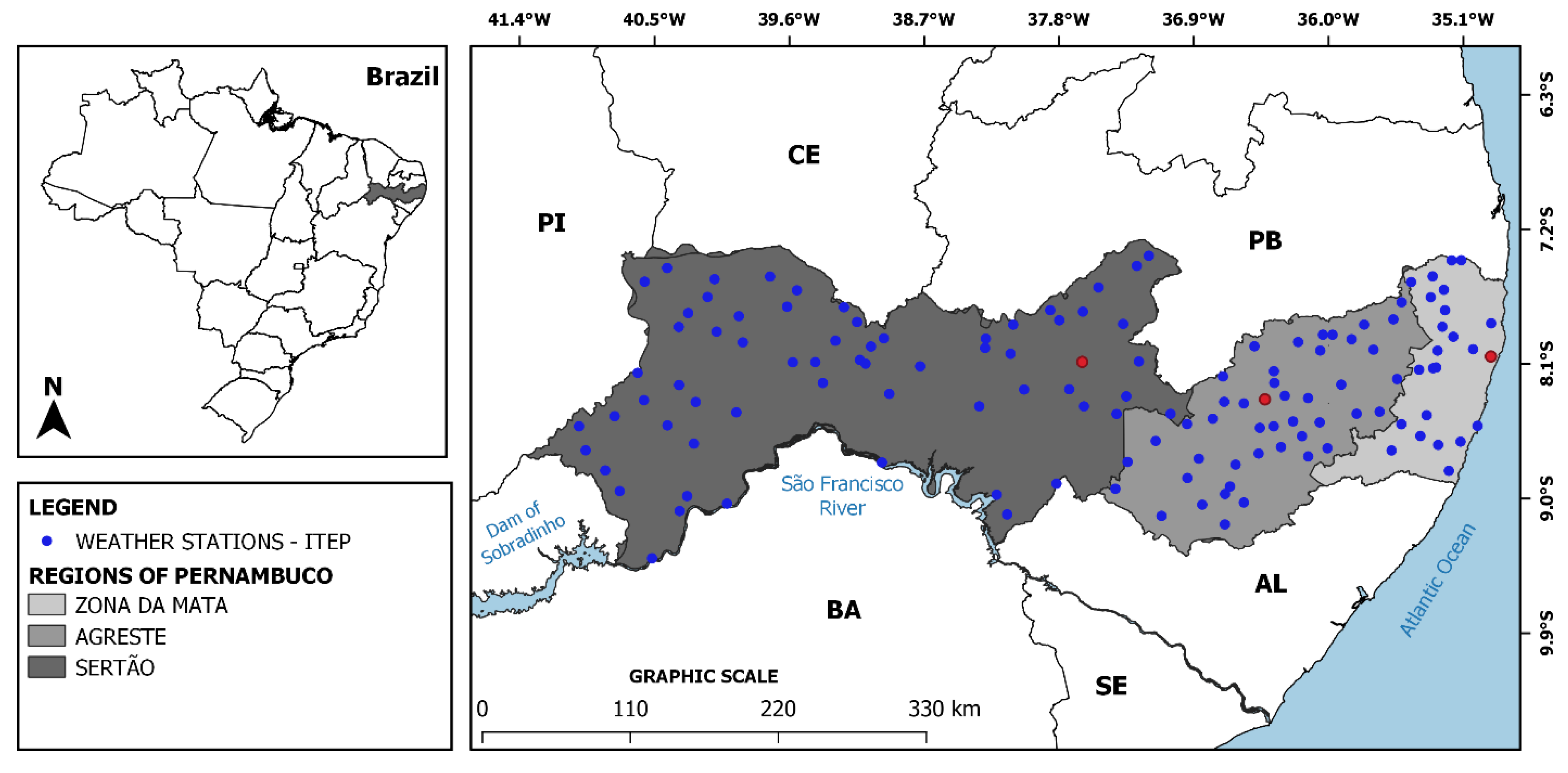
Pernambuco is a state located in the eastern part of the NEB, between the parallels 7° 15′45″ S and 9°28′18″ S and meridians 34°48′33″ W and 41°19′54″ W. It is bordered by the states of Alagoas and Bahia (south), Piaui (west), Paraiba and Ceará (north), and the Atlantic Ocean in the east (Figure 1). Pernambuco is divided into three geographical regions: the Atlantic Forest zone (Zona da Mata), which stretches approximately 70 km from the sea to the Borborema mountain chain, a subhumid transition zone (Agreste), and, to the west of the Borborema chain, the largest semiarid region (Sertão).

The coastal region of Zona da Mata is covered by small patches of Atlantic rainforest, mostly on the tops of low hills (50–100 m high), and sugar cane fields at lower elevations. Caatinga is a semiarid biome dominated by tropical dry forest, pastures, and agricultural fields of subsistence crops (maize, beans, and cassava) that covers the majority of the Sertão region, while both the Atlantic Forest and Caatinga coexist in the transition zone of Agreste [46,47]. The climate in the coastal region is tropical humid with a rainfall gradient from east (1500 mm) to west (700 mm), a rainy season from May to July, and a dry season from September to December.

Sertão has a semiarid climate with less than 500 mm of precipitation annually, concentrated between February and April, and for the rest of the year, 9 months of dry weather [48]. Pernambuco is affected by both the droughts in Sertão and the floods in the coastal area, which increase risks to water, energy, food security, and natural hazards such as flash floods and landslides, and these conditions are expected to become more severe until the end of the century due to climate change. Future projections of those risks depend on the reliability of information about future trends in regional precipitation, which is the main climatic variable used in the modeling of water-related risk indices such as the aridity index, and the flash floods and landslides vulnerability indices [3,49].

2.2. Data

The data used in this work are monthly precipitation time series recorded during the period from 1962 to 2012 at 133 meteorological stations in the state of Pernambuco, Brazil, which are shown in Figure 1. Data are provided by the Meteorological Laboratory of the Institute of Technology of Pernambuco (Laboratório de Meteorologia do Instituto de Tecnologia de Pernambuco—LAMEP/ITEP). More details about this dataset can be found in ref. [50].

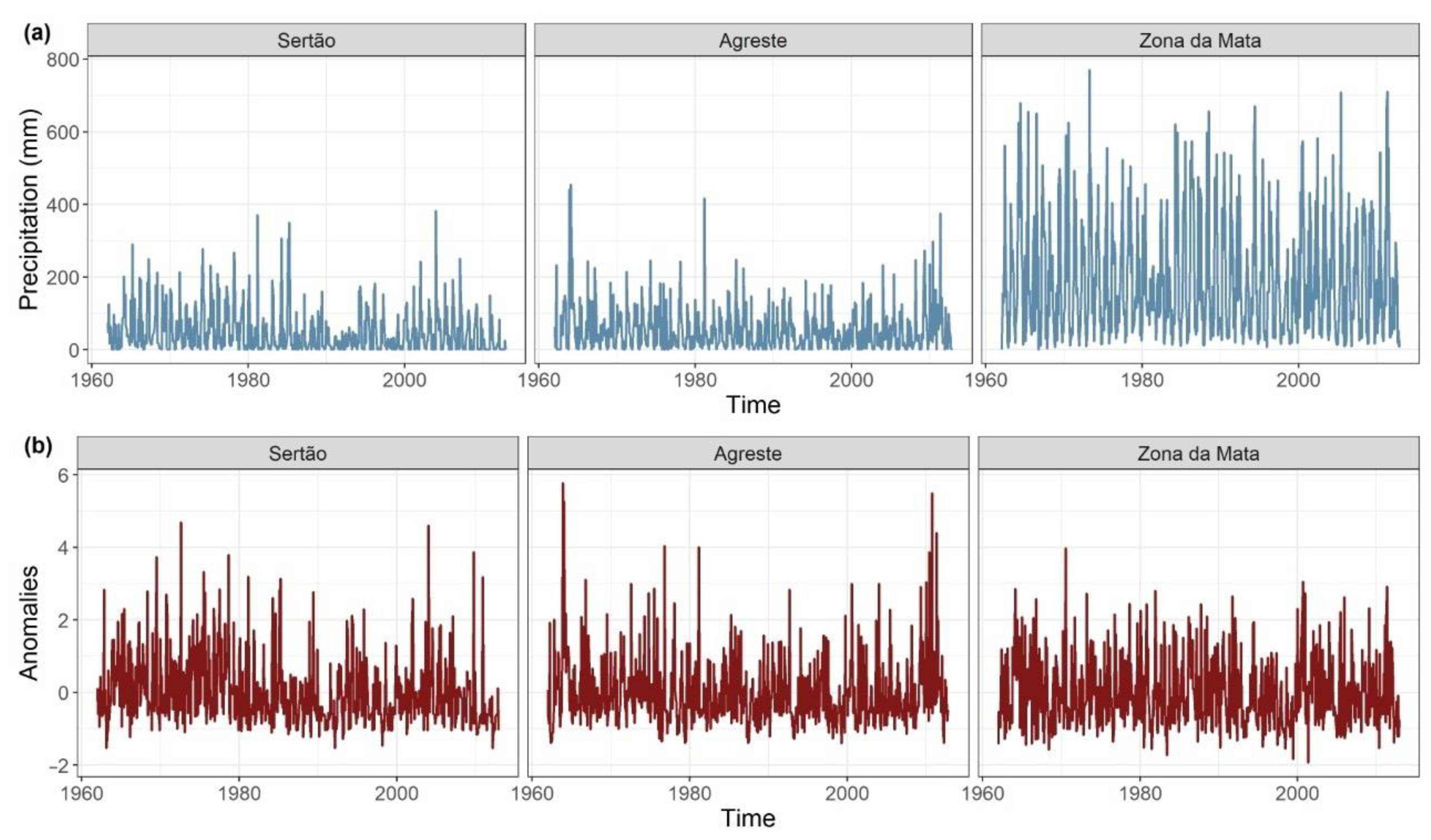
The original and deseasonalized (anomalies) monthly rainfall series for three representative stations, chosen to illustrate the rainfall regime in different climatic zones, are shown in Figure 2. The rainfall anomalies are calculated as

$$X\left(t\right)=\left(x\left(t\right)-{\mu }_t\right)/{\sigma }_t$$

where ${\mu }_t$ and ${\sigma }_t$ are the mean and the standard deviation of monthly rainfall $x\left(t\right)$, calculated for each calendar month by averaging over all the years in the record.

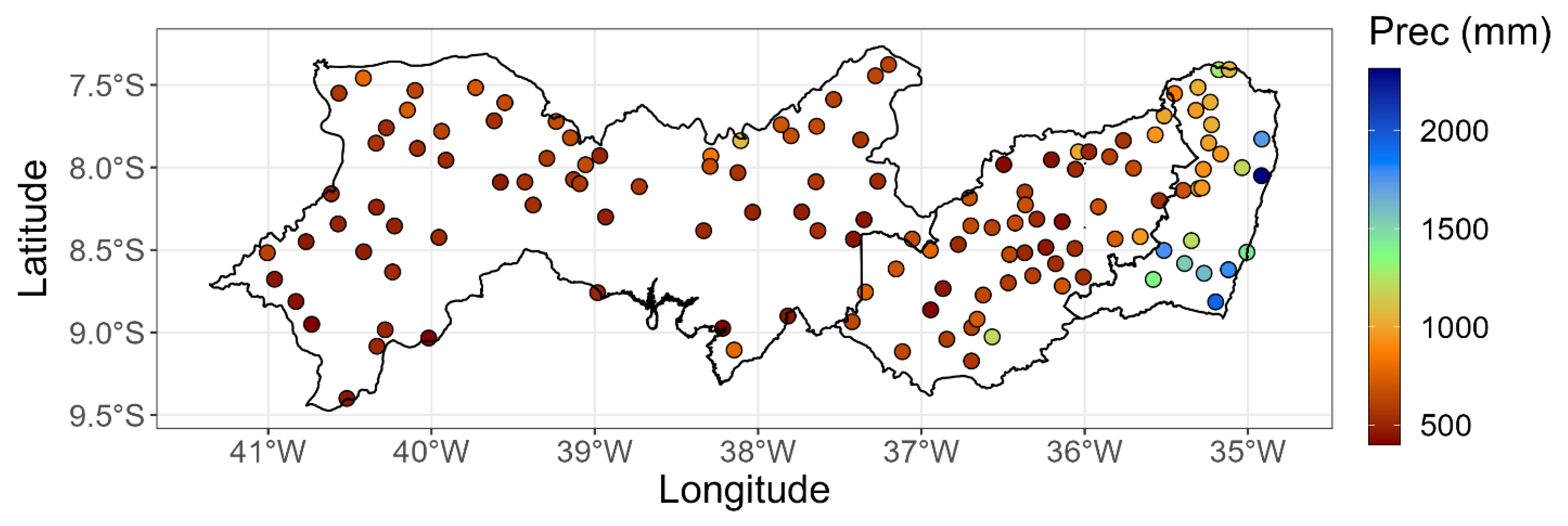
The spatial distribution of the mean annual accumulated rainfall over the state of Pernambuco is shown in Figure 3, where a clear pattern can be observed: the decrease in annual rainfall amounts in the east–west direction, more rainfall in the costal Zona de Mata region, much less rain in the inland semiarid Sertão region, and intermediate rainfall amounts in the transition Agreste region.

This pattern can also be observed in the rainfall series for three representative stations in Figure 2a. The anomalies series (Figure 2b) show more erratic behavior for Sertão and Agreste, where (especially in Sertão) droughts are more pronounced than in Zona de Mata, where the anomalies series are more uniform throughout the analyzed period.

2.3. Sample Entropy (SampEn)

Richman and Moorman [40] introduced sample entropy (SampEn) as a measure of the rate at which new information is generated in a temporal series. $SampEn\left(m,r,N\right)$ is defined as the negative natural logarithm of the conditional probability that two sequences that are similar at $m$ points remain similar at $m+1$ points, assuming that self-matches are excluded from the probability calculation. $SampEn$ can be used to describe the regularity of temporal series, as it has lower values for time series with more frequent occurrence of sequences of similar consecutive values. Sample entropy method was used in physiology [51,52], geophysics [53], climatology [54], hydrology [30,34,35], and engineering [55].

Sample entropy algorithm can be described through the following steps [40]:

• For a time series $u\left(i\right),i=1,\dots ,N$ of length $N$, one first forms m—dimensional template vectors $x_m\left(i\right)=\left\{u\left(i+k\right):k=0,\dots ,m-1\right\},i=1,\dots ,N-m+1$;
• The distance between two vectors $x_m\left(i\right)$ and $x_m\left(j\right)$ is defined as the maximum difference of their corresponding scalar components;
• $d[x_m\left(i\right)$,$x_m\left(j\right)]=\max \left\{\left|u\left(i+k\right)-u\left(j+k\right)\right|:k=0,\dots ,m-1\right\}$;
• One then counts the number $B_i$ of vectors $x_m\left(j\right)$ which are similar to $x_m\left(i\right)$ within the tolerance level $r$: $d[x_m\left(i\right)$,$x_m\left(j\right)\le r,r=r\sigma$ ($\sigma$—standard deviation of $u\left(i\right),i=1,\dots ,N$) and $j\ne i$ to exclude self-matches;
• Defining $B_i^m\left(r\right)=\frac{B_i}{N-m+1}$, the probability that two vectors will match for n points is given by $B^m\left(r\right)=\frac{{{\displaystyle \sum }}_{i=1}^{N-m}{B}_i^m\left(r\right)}{N-m}$;
• The steps i-iv are then repeated for vectors of length $m+1$, defining $A_i^m\left(r\right)=\frac{A_i}{N-m+1}$ and $A^m\left(r\right)=\frac{{{\displaystyle \sum }}_{i=1}^{N-m}{A}_i^m\left(r\right)}{N-m}$, where $A_i$ is a number of vectors $x_{m+1}\left(j\right)$ which are similar (at tolerance level $r$) to $x_{m+1}\left(i\right)$, and $A^m\left(r\right)$ is the probability that two vectors will match for $m+1$ points;
• Finally, sample entropy (SampEn) is defined as

  $$S_E\left(m,r\right)=\underset{N\to \infty }{\lim }\left[-ln\frac{A^m\left(r\right)}{B^m\left(r\right)}\right]$$

  and can be estimated by the statistics

  $$S_E\left(m,r\right)=-ln\frac{A^m\left(r\right)}{B^m\left(r\right)}$$

SampEn can be expressed as $-ln\left(A/B\right)$ where $A$ and $B$ are the total number of forward template matches of length $m+1$ ad $m$, respectively [40].

Sample entropy can also be calculated with template vectors that are defined with time delay $\delta$: $x_m^{\delta }\left(i\right)=\left\{u\left(i\right)u\left(i+\delta \right)\dots u\left(i+\left(m-1\right)\delta \right)\right\}$, $i=1,\dots ,N-\left(m-1\right)\delta$ [56]. The SampEn parameters chosen in this study are $m=2$, $r=0.2$ [40], and different values of $\delta$ for different time scales [45].

2.4. Multiscale Entropy (MSE)

Costa et al. [39] introduced the concept of multiscale sample entropy (MSE) by calculating sample entropy for consecutive coarse-grained time series $x_{\tau }\left(j\right)=\frac{1}{\tau }{{\displaystyle \sum }}_{i=\left(j-1\right)\tau +1}^{j\tau }u\left(i\right)$ where $j=1,\dots ,N/\tau$, $u\left(i\right),i=1,\dots ,N$ denotes the initial time series and τ is a scale factor. MSE is obtained by plotting SampEn values for each scale factor $\tau$, and is more suitable for quantifying complexity in short and noisy time series than traditional entropy methods that are based on pattern repetition on a single temporal scale [39]. MSE method was successfully used in analyzing physiological signals [57,58], geophysical records [59], hydrological processes [41,42,43], and financial time series [60,61].

2.5. Modified Multiscale Entropy (MMSE)

MSE estimation is imprecise for short time series because the coarse-graining procedure reduces the length of the original time series by a scale factor τ. Several alternative coarse graining procedures have been proposed to improve the reliability of MSE [62]. In this work we use the modified multiscale entropy (MMSE) [45], in which the moving average procedure is used for coarse graining ($x_{\tau }\left(j\right)=\frac{1}{\tau }{{\displaystyle \sum }}_{i=j}^{j+\tau }u\left(i\right)$, $j=1,\dots ,N-\tau$ + 1) and for each time scale $\tau$ sample entropy is calculated with a time delay $\delta =\tau$, i.e., using template vectors $x_m^{\tau }\left(i\right)=\left\{x\left(i\right)x\left(i+\tau \right)\dots x\left(i+\left(m-1\right)\tau \right)\right\}$.

3. Results and Discussion

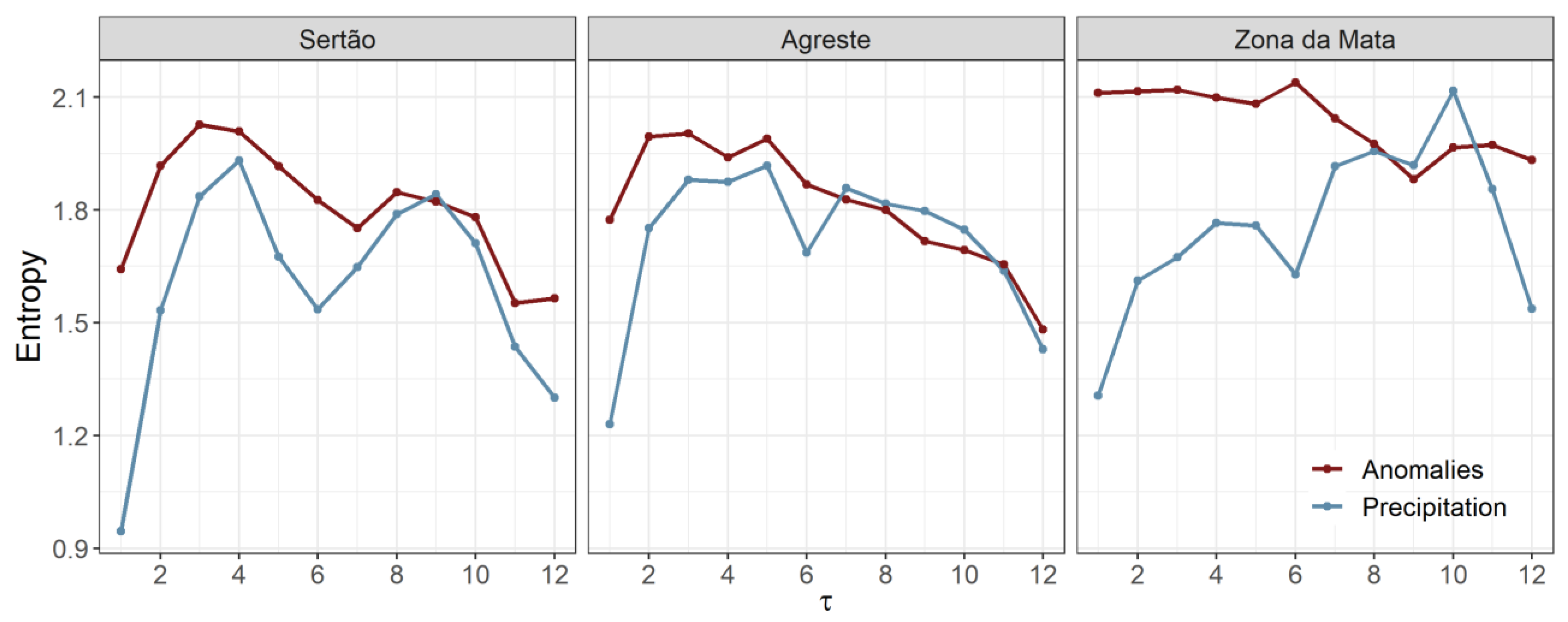
The results for the MMSE values for $\tau$ = 1, 2,…, 12, for the original series and anomalies for three representative stations are shown in Figure 4, where several patterns can be observed. For the low and intermediate scales (due to intra annual variability), the original series show lower entropy values, indicating more regularity and more predictability than the anomaly series. This difference diminishes on higher temporal scales, except for $\tau$ = 12 for Sertão and Zona de Mata, which reflects annual seasonality.

For both the smallest ($\tau$ = 1) and the largest ($\tau$ = 12) temporal scales, the lowest entropy values for the original series are found for the Sertão region due to the most pronounced separation of the dry and rainy seasons. More precisely, the dry season in Sertão lasts 9 months, resulting in high monthly regularity and low entropy for $\tau$ = 1, while the strong annual seasonality results in low entropy for $\tau$ = 12. For all regions, the original series display lower entropy for $\tau$ = 1 than for $\tau$ = 12 indicating that intra-annual regularity is more pronounced than interannual seasonality, and this difference is larger for Sertão. Besides these two scales, in all cases, lower entropy is also observed at $\tau$ = 6, indicating that all three regions show a certain type of synchronization in the rainfall regime when the average monthly rainfall amount calculated over a 6-month period is observed.

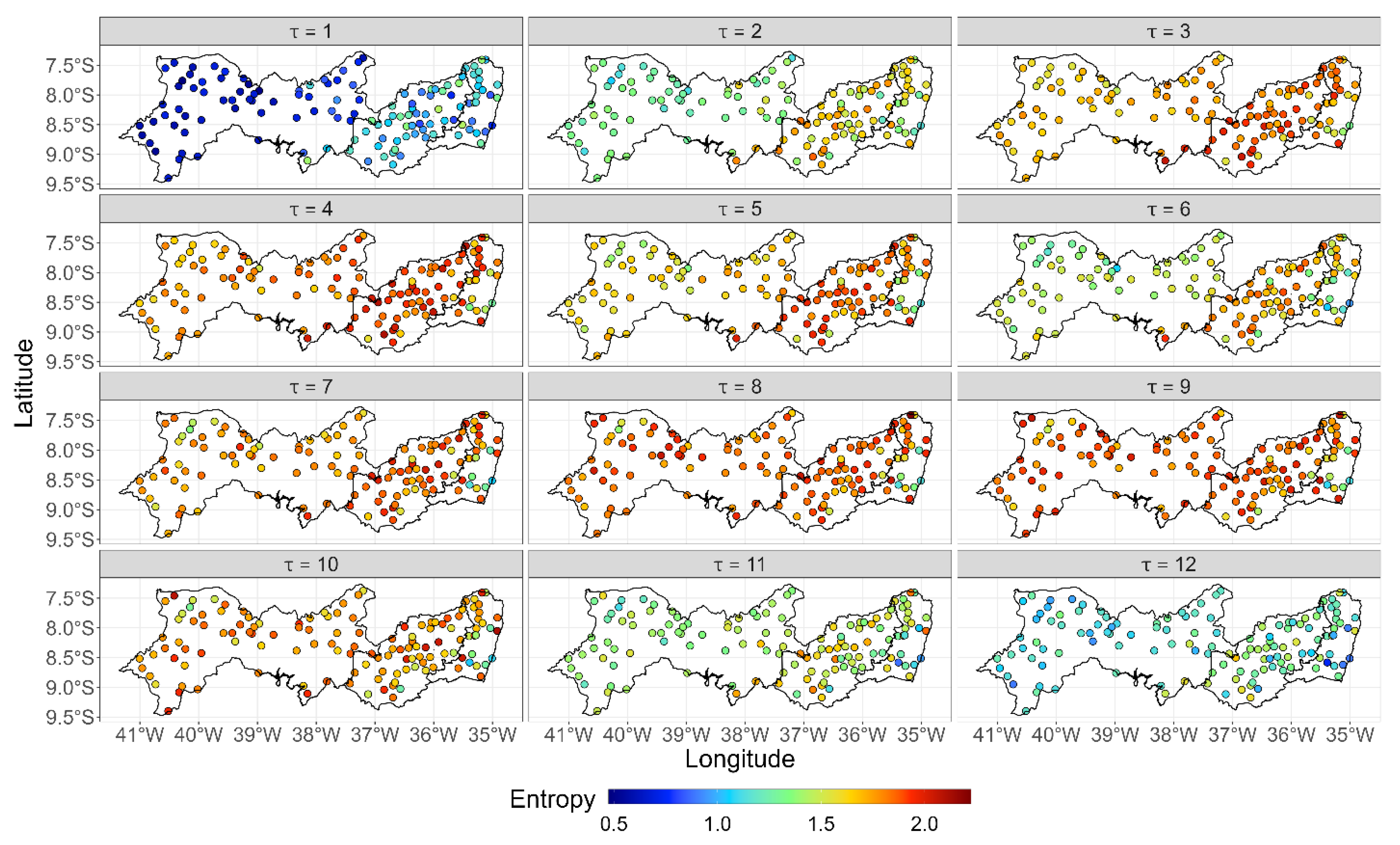
The spatial distribution of the MMSE values for the original and the anomaly series across the state of Pernambuco, obtained for all 133 stations, are shown in Figure 5 and Figure 6, respectively. Besides confirming the results for the representative stations shown in Figure 4 (higher entropy for the anomaly series, as well as lower entropy for the original series for the temporal scales $\tau$ = 1, $\tau$ = 6, and $\tau$ = 12), we can observe more detailed spatial patterns for each temporal scale.

For the original series (Figure 5), for $\tau$ = 1 the entropy increases in the west–east direction, indicating the highest regularity and predictability of rainfall dynamics in the deep inland Sertão region, and the lowest regularity and predictability in the coastal region. For higher temporal scales ($\tau$ = 2, …, 12), the entropy values increase from Sertão towards Agreste, and then decrease towards the coast, indicating that the rainfall regime is the most irregular and the least predictable in the Agreste region, which is a climate transition zone.

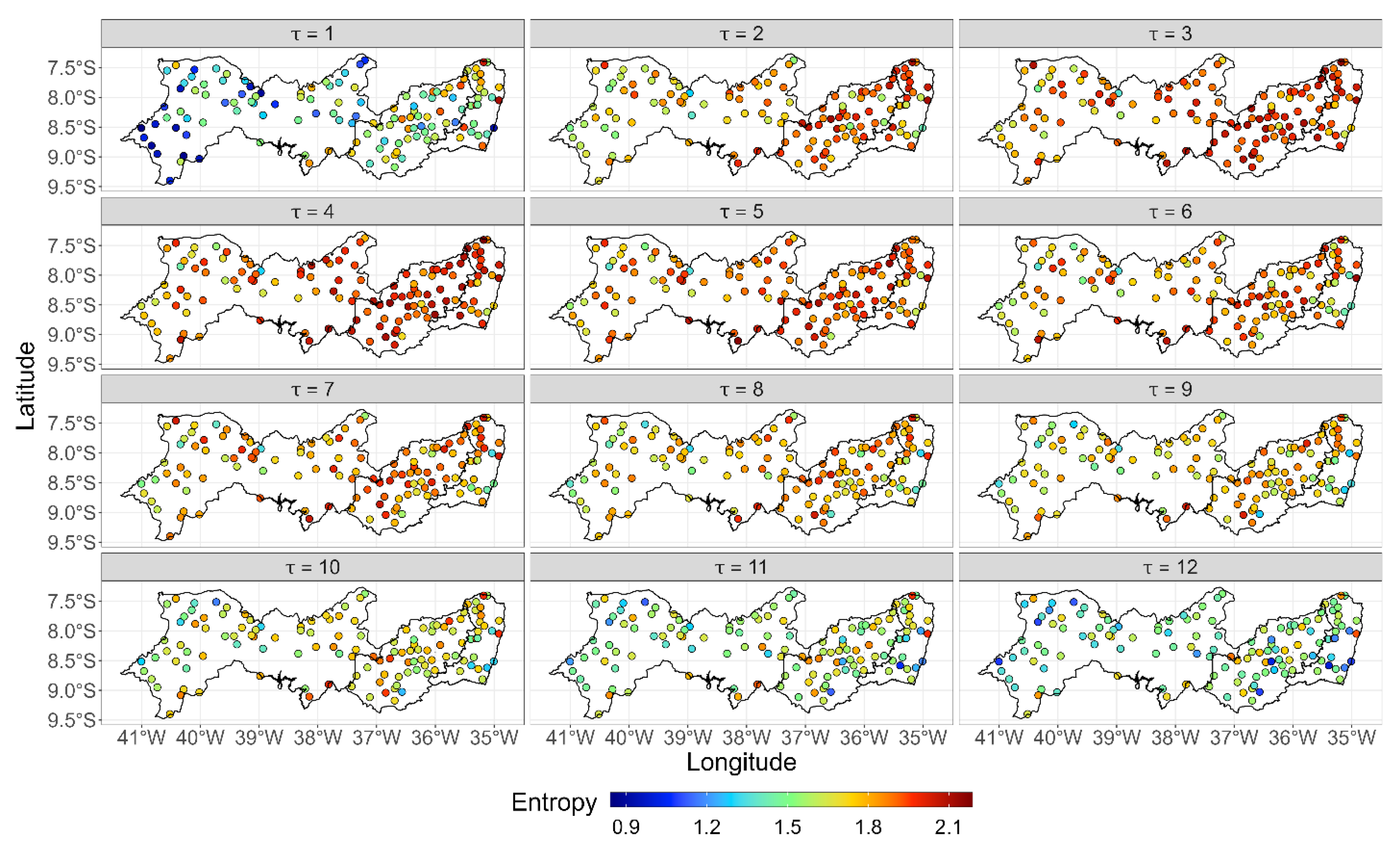
For rainfall anomalies (Figure 6), the difference between the MMSE values for three regions is less pronounced, as yearly seasonality is removed. Still, the lowest entropy values are observed for the smallest ($\tau$ = 1) and the highest ($\tau$ = 12) temporal scales. Considering the whole Pernambuco region, we observe the increase of entropy values until the scale of 4 months ($\tau$ = 4), and then the entropy decreases with scale, reaching the lowest values for $\tau$ = 12. For the original series (Figure 5), we observe several ranges of scale with an alternating tendency in entropy values: increasing until $\tau$ = 4, then decreasing until $\tau$ = 6, increasing until $\tau$ = 9, and decreasing until reaches the lowest values for $\tau$ = 12.

These temporal scales are related to the intra-annual variability of rainfall in Pernambuco: in Zona de Mata, the rainy season is concentrated in three months between May and July, and the intense dry season in four months between September and December; in the Sertão region, the rainy season is concentrated in three months from February to April, and a dry period that lasts nine months [48]; in Agreste, the dry season is concentrated in five months between August and December [63]. The scale $\tau$ = 12 reflects annual seasonality.

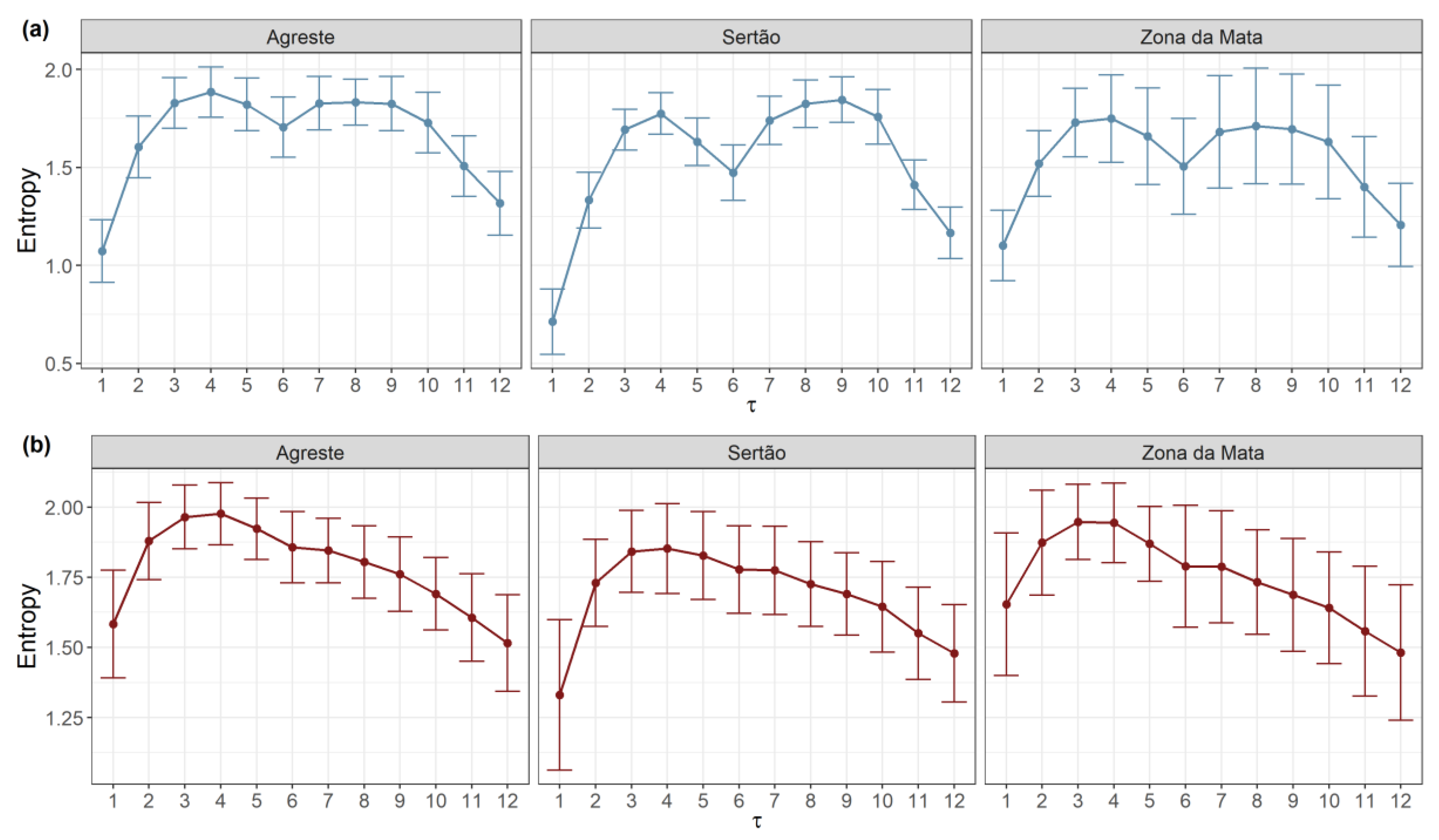
Figure 7 shows the average MMSE curve together with standard deviation calculated for the rainfall original series and rainfall anomalies for Zona de Mata, Agreste, and Sertão stations. It is seen that these curves are much smoother than those for the individual stations shown in Figure 4, but the general observation for the original series still holds: the lowest entropies for the 1-month and 12-month scale and “local minimum” for the 6-month scale.

For the anomalies series, the averaging over all the stations within the regions also produced a clear MMSE pattern: the increase in entropy until the scale of 4 months and then a decrease until the highest scale of 12 months, as seen in Figure 6. The values of the average MMSE and standard deviation for each region and each temporal scale, used to produce Figure 5 and Figure 6, are presented in

Table 1. Average MMSE values (together with standard deviation) for rainfall temporal series.

	Region
$\mathit{\tau }$	Agreste		Sertão		Zona da Mata
	$\overline{\mathit{x}}$	sd	$\overline{\mathit{x}}$	sd	$\overline{\mathit{x}}$	$sd$
1	1.074	0.160	0.713	0.166	1.101	0.180
2	1.605	0.157	1.333	0.142	1.519	0.167
3	1.828	0.129	1.692	0.104	1.729	0.175
4	1.884	0.128	1.775	0.106	1.750	0.223
5	1.821	0.134	1.631	0.121	1.659	0.246
6	1.706	0.154	1.472	0.142	1.506	0.243
7	1.828	0.136	1.740	0.122	1.680	0.286
8	1.833	0.118	1.825	0.121	1.711	0.294
9	1.825	0.138	1.846	0.117	1.696	0.281
10	1.728	0.154	1.758	0.139	1.630	0.290
11	1.507	0.155	1.411	0.126	1.400	0.256
12	1.317	0.163	1.166	0.131	1.207	0.212

and

Table 2. Average MMSE values (together with standard deviation) for rainfall anomalies series.

	Region
$\mathit{\tau }$	Agreste		Sertão		Zona da Mata
	$\overline{\mathit{x}}$	sd	$\overline{\mathit{x}}$	sd	$\overline{\mathit{x}}$	sd
1	1.583	0.192	1.331	0.268	1.654	0.254
2	1.880	0.138	1.730	0.156	1.874	0.187
3	1.965	0.114	1.842	0.147	1.948	0.134
4	1.977	0.110	1.852	0.160	1.944	0.142
5	1.924	0.109	1.828	0.157	1.870	0.133
6	1.858	0.127	1.778	0.156	1.789	0.217
7	1.846	0.115	1.775	0.158	1.788	0.200
8	1.804	0.129	1.726	0.151	1.733	0.186
9	1.761	0.133	1.691	0.147	1.688	0.201
10	1.691	0.130	1.645	0.162	1.641	0.199
11	1.606	0.156	1.550	0.164	1.558	0.232
12	1.516	0.173	1.479	0.173	1.482	0.242

, respectively.

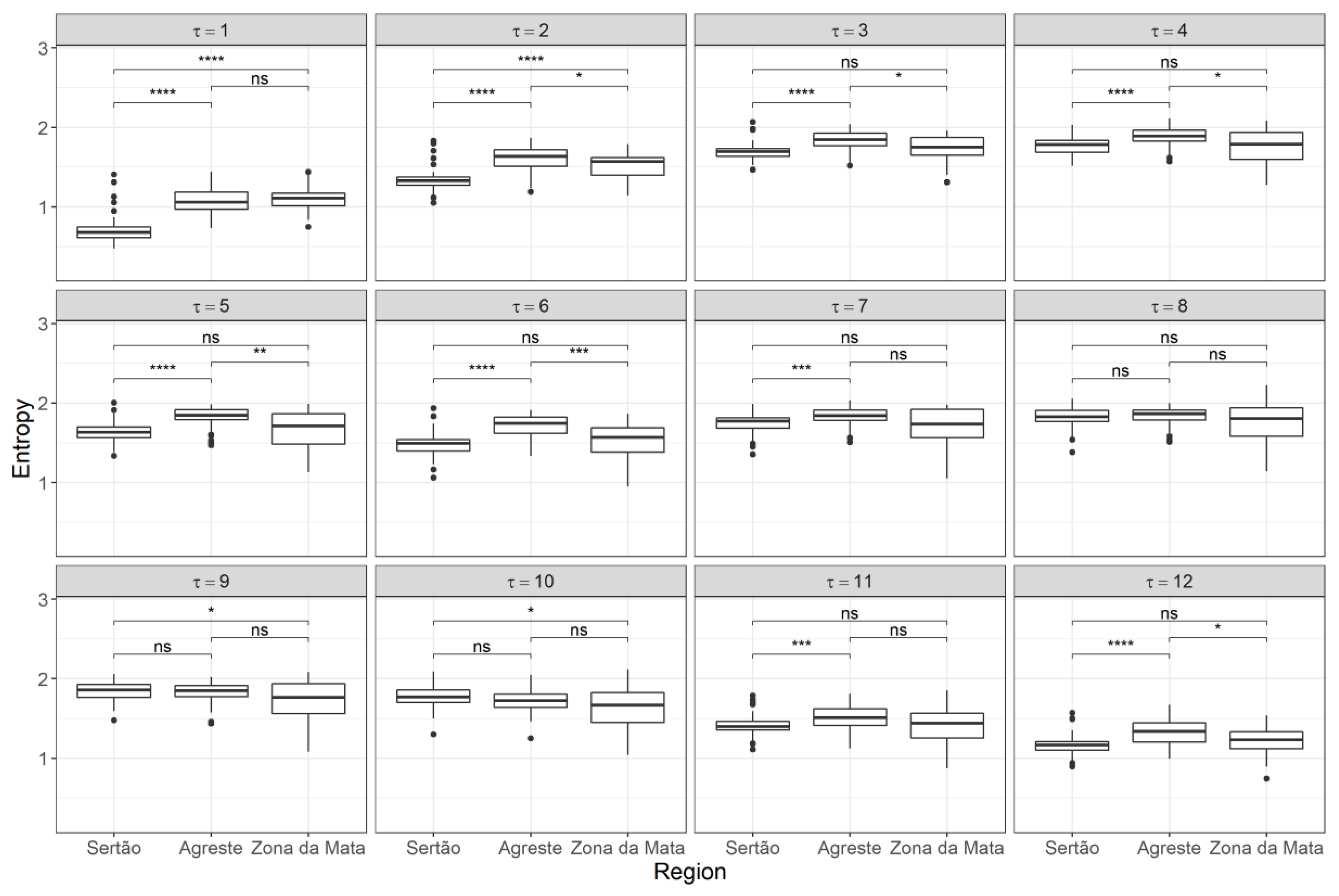
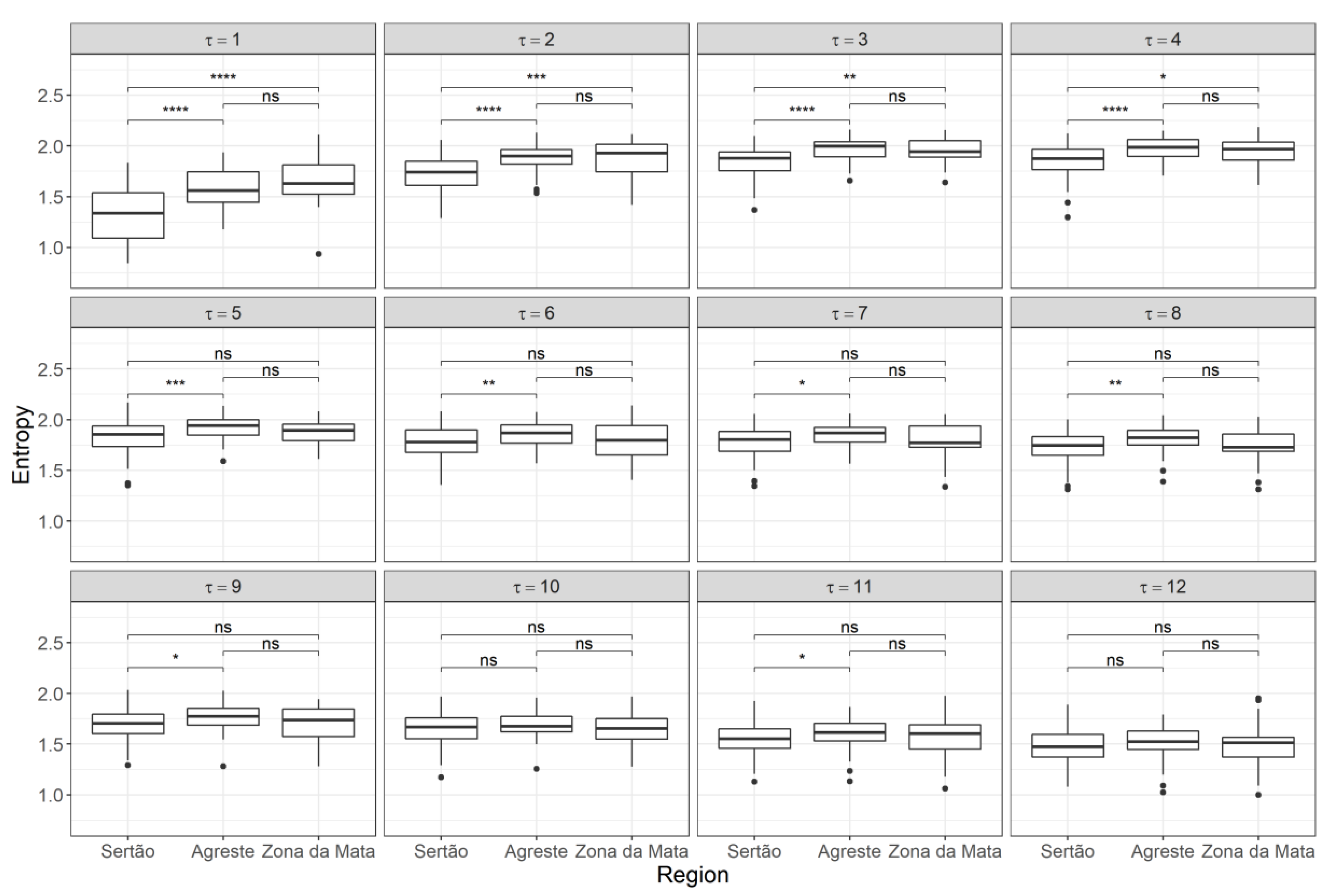
In order to assess the difference in the MMSE values between the three regions, we apply the Wilcoxon-Mann-Whitney test (at the 5% significance level) to each temporal scale τ = 1, 2, …, 12. The results for the original and anomaly series are shown in Figure 8 and Figure 9, respectively.

It is seen from Figure 8 that, for the original series, a significant difference between Sertão and Zona de Mata is found for τ = 1, 2, 9, 10; between Sertão and Agreste for τ = 1, 2, 3, 4, 5, 6, 7, 11, 12, and between Agreste and Zona de Mata for τ = 2, 3, 4, 5, 6, 12. For the anomalies series (Figure 9), the significant difference between Sertão and Zona de Mata is found for τ = 1, 2, 3, 4; between Sertão and Agreste for τ = 1, 2, 3, 4, 5, 6, 7, 8, 9, 11, while between Agreste and Zona de Mata the MMSE values do not show a significant difference.

It is expected that the anomaly series are less sensitive to SampEn analysis, besides showing higher entropy values due to the removed seasonality component, and for Agreste/Zona de Mata they show a similar level of regularity. However, for Sertão/Zona de Mata, a significant difference is found for the same number of scales as for the original series (4), and almost the same for Sertão/Agreste (9 scales for the original series and 10 scales for the anomalies series).

This result may seem surprising, as it is known that among the three regions the amount and distribution of rain during the year is most different between Sertão and Zona de Mata, and the MMSE analysis shows more difference for Sertão/Agreste and Agreste/Zona de Mata for the original series, and for Sertão/Agreste for anomalies series. This finding can be attributed to the fact that SampEn evaluates the regularity of temporal series independently if that regularity is the result of long periods of dry or wet months, and the two rainfall temporal series that have a similar level of “uniformity” may produce similar SampEn values independently of the underlying values of the rainfall amount.

4. Conclusions

In this work, we analyzed the complexity of monthly rainfall series from 133 pluviometric stations from the state of Pernambuco, Brazil, in order to compare the rainfall regimes in three regions: Zona da Mata, Agreste, and Sertão. We applied the method of modified multiscale entropy (MMSE), which evaluates the regularity of temporal series on different temporal scales and is suitable for short time series.

For each rainfall series, we calculated the MMSE values for 12 temporal scales (1–12 months) for the original series and anomalies. For the original series for temporal scale τ = 1, the entropy increased in the west–east direction, indicating the highest regularity and the highest predictability of rainfall dynamics in the deep inland Sertão region, and the lowest regularity and the lowest predictability in the coastal region. For other temporal scales (τ = 2, …, 12), the entropy values increased from Sertão towards Agreste and then decreased toward the coast, indicating that the rainfall regime is most irregular and the least predictable in the transition zone of Agreste.

For all regions, lower entropy values were found for τ = 1 and τ = 12, reflecting intra-annual rainfall variability (well-defined dry and wet seasons) and interannual seasonality, respectively. This effect was less pronounced for rainfall anomalies where seasonality is removed. For intra-annual temporal scales for Sertão, the entropy values of the anomaly series were lower for τ = 3 and τ = 9, which can be attributed to the duration of the wet (3 months) and dry (9 months) seasons.

We also performed a statistical significance test to compare the MMSE values in three regions, and found that, for the original series for most temporal scales, there was a significant difference in the MMSE values (rainfall regularity) between Sertão and Agreste, and Agreste and Zona de Mata. For the anomalies series, a significant difference was found between Sertão and Agreste, but not between Agreste and Zona de Mata. The significant difference between the MMSE values for Sertão and Zona da Mata was found on a limited number of temporal scales.

Although the climate and the amount of annual rainfall are different in these two distant regions, the rainfall regularity is similar due to strong intra-annual seasonality (3 months of wet season). The applications of multiscale entropy in hydrology have been limited to the analysis of streamflow data, and have been shown to be useful for detecting hydrological changes caused by human activities such as dam and reservoir construction [42,43]

Rainfall data were studied with the sample entropy method that evaluates regularity on a temporal scale τ = 1 [30,34,35], while the comprehensive studies on rainfall multiscale dynamics are still ongoing. By using the MMSE method, we obtained entropy values over a wide range of temporal scales, from 1 month to 1 year, which provided a more complete description of rainfall complexity than when analyzed on a single temporal scale.

Our results indicate that a multiscale approach to the analysis of rainfall data can be used to compare the rainfall regimes at different temporal scales and contributes to a better understanding of the mechanisms governing climate dynamics.

References

- Marengo, J.A.; Torres, R.R.; Alves, L.M. Drought in Northeast Brazil—past, present, and future. Theor. Appl. Climatol. 2017, 129, 1189–1200. [Google Scholar] [CrossRef]
- Cunha, A.P.M.A.; Tomasella, J.; Ribeiro-Neto, G.G.; Brown, M.; Garcia, S.R.; Brito, S.B.; Carvalho, M.A. Changes in the spatial–temporal patterns of droughts in the Brazilian Northeast. Atmos. Sci. Lett. 2018, 19, e855. [Google Scholar] [CrossRef] [Green Version]
- Marengo, J.A.; Bernasconi, M. Regional differences in aridity/drought conditions over Northeast Brazil: Present state and future projections. Clim. Chang. 2015, 129, 103–115. [Google Scholar] [CrossRef]
- Hastenrath, S.; Greischar, L. Circulation mechanisms related to Northeast Brazil rainfall anomalies. J. Geophys. Res. Atmos. 1993, 98, 5093–5102. [Google Scholar] [CrossRef]
- Andreoli, R.V.; Kayano, M.T. Tropical Pacific and South Atlantic effects on rainfall variability over Northeast Brazil. Int. J. Climatol. 2006, 26, 1895–1912. [Google Scholar] [CrossRef]
- De Lima Moscati, M.C.; Gan, M.A. Rainfall variability in the rainy season of semiarid zone of Northeast Brazil (NEB) and its relation to wind regime. Int. J. Climatol. 2007, 27, 493–512. [Google Scholar] [CrossRef]
- Liebmann, B.; Kiladis, G.N.; Allured, D.; Vera, C.S.; Jones, C.; Carvalho, L.M.V.; Bladé, I.; Gonzáles, P.L.M. Mechanisms associated with large daily rainfall events in Northeast Brazil. J. Clim. 2011, 24, 376–396. [Google Scholar] [CrossRef] [Green Version]
- Oliveira, P.T.; Santos e Silva, C.M.; Lima, K.C. Climatology and trend analysis of extreme precipitation in subregions of Northeast Brazil. Theor. Appl. Climatol. 2017, 130, 77–90. [Google Scholar] [CrossRef]
- Rodrigues, D.T.; Gonçalves, W.A.; Spyrides, M.H.C.; Santos e Silva, C.M.; Souza, D.O. Spatial distribution of the level of return of extreme precipitation events in Northeast Brazil. Int. J. Climatol. 2020, 40, 5098–5113. [Google Scholar] [CrossRef]
- Uvo, C.; Berndtsson, R. Regionalization and spatial properties of Ceará State rainfall in Northeast Brazil. J. Geophys. Res. Atmos. 1996, 101, 4221–4233. [Google Scholar] [CrossRef] [Green Version]
- Lyra, G.B.; Oliveira-Júnior, J.F.; Zeri, M. Cluster analysis applied to the spatial and temporal variability of monthly rainfall in Alagoas state, Northeast of Brazil. Int. J. Climatol. 2014, 34, 3546–3558. [Google Scholar] [CrossRef]
- Silva, B.K.N.; Lucio, P.S. Characterization of risk/exposure to climate extremes for the Brazilian Northeast—case study: Rio Grande do Norte. Theor. Appl. Climatol. 2015, 122, 59–67. [Google Scholar] [CrossRef]
- Medeiros, E.S.D.; Lima, R.R.D.; Olinda, R.A.D.; Santos, C.A.C.D. Modeling spatiotemporal rainfall variability in Paraíba, Brazil. Water 2019, 11, 1843. [Google Scholar] [CrossRef] [Green Version]
- Buytaert, W.; Celleri, R.; Willems, P.; De Bievre, B.; Wyseure, G. Spatial and temporal rainfall variability in mountainous areas: A case study from the south Ecuadorian Andes. J. Hydrol. 2006, 329, 413–421. [Google Scholar] [CrossRef]
- Longobardi, A.; Villani, P. Trend analysis of annual and seasonal rainfall time series in the Mediterranean area. Int. J. Climatol. 2010, 30, 1538–1546. [Google Scholar] [CrossRef]
- Gebrechorkos, S.H.; Hülsmann, S.; Bernhofer, C. Long-term trends in rainfall and temperature using high-resolution climate datasets in East Africa. Sci. Rep. 2019, 9, 11376. [Google Scholar] [CrossRef] [PubMed] [Green Version]
- Douka, M.; Karacostas, T. Statistical analyses of extreme rainfall events in Thessaloniki, Greece. Atmos. Res. 2018, 208, 60–77. [Google Scholar] [CrossRef]
- Blanchet, J.; Molinié, G.; Touati, J. Spatial analysis of trend in extreme daily rainfall in southern France. Clim. Dyn. 2018, 51, 799–812. [Google Scholar] [CrossRef]
- Camberlin, P.; Barraud, G.; Bigot, S.; Dewitte, O.; Makanzu Imwangana, F.; Maki Mateso, J.; Martiny, N.; Monsieurs, E.; Moron, V.; Pellarin, T.; et al. Evaluation of remotely sensed rainfall products over Central Africa. Q. J. R. Meteorol. Soc. 2019, 145, 2115–2138. [Google Scholar] [CrossRef]
- Neto, R.M.B.; Santos, C.A.G.; da Costa, J.F.C.B.; da Silva, R.M.; Dos Santos, C.A.C.; Mishra, M. Evaluation of the TRMM product for monitoring drought over Paraíba State, northeastern Brazil: A trend analysis. Sci. Rep. 2021, 11, 1097. [Google Scholar] [CrossRef]
- Bosilovich, M.G.; Chen, J.; Robertson, F.R.; Adler, R.F. Evaluation of global precipitation in reanalyses. J. Appl. Meteorol. Climatol. 2008, 47, 2279–2299. [Google Scholar] [CrossRef]
- Tessier, Y.; Lovejoy, S.; Hubert, P.; Schertzer, D.; Pecknold, S. Multifractal analysis and modeling of rainfall and river flows and scaling, causal transfer functions. J. Geophys. Res. Atmos. 1996, 101, 26427–26440. [Google Scholar] [CrossRef]
- Kantelhardt, J.W.; Koscielny-Bunde, E.; Rybski, D.; Braun, P.; Bunde, A.; Havlin, S. Long-term persistence and multifractality of precipitation and river runoff records. J. Geophys. Res. Atmos. 2006, 111. [Google Scholar] [CrossRef]
- Tan, X.; Gan, T.Y. Multifractality of Canadian precipitation and streamflow. Int. J. Climatol. 2017, 37, 1221–1236. [Google Scholar] [CrossRef]
- Adarsh, S.; Nourani, V.; Archana, D.S.; Dharan, D.S. Multifractal description of daily rainfall fields over India. J. Hydrol. 2020, 586, 124913. [Google Scholar] [CrossRef]
- Fuwape, I.A.; Ogunjo, S.T.; Oluyamo, S.S.; Rabiu, A.B. Spatial variation of deterministic chaos in mean daily temperature and rainfall over Nigeria. Theor. Appl. Climatol. 2017, 130, 119–132. [Google Scholar] [CrossRef]
- Sivakumar, B. Nonlinear dynamics and chaos in hydrologic systems: Latest developments and a look forward. Stoch. Environ. Res. Risk Assess. 2009, 23, 1027–1036. [Google Scholar] [CrossRef]
- Mishra, A.K.; Özger, M.; Singh, V.P. An entropy-based investigation into the variability of precipitation. J. Hydrol. 2009, 370, 139–154. [Google Scholar] [CrossRef]
- Pierini, J.O.; Scian, B.; Lovallo, M.; Telesca, L. Discriminating climatological regimes in rainfall time series by using the Fisher-Shannon method. Int. J. Phys. Sci. 2011, 6, 7799–7804. [Google Scholar]
- Xavier, S.F.A.; da Silva Jale, J.; Stosic, T.; dos Santos, C.A.C.; Singh, V.P. An application of sample entropy to precipitation in Paraíba State, Brazil. Theor. Appl. Climatol. 2019, 136, 429–440. [Google Scholar] [CrossRef]
- Malik, N.; Bookhagen, B.; Marwan, N.; Kurths, J. Analysis of spatial and temporal extreme monsoonal rainfall over South Asia using complex networks. Clim. Dyn. 2012, 39, 971–987. [Google Scholar] [CrossRef]
- Boers, N.; Bookhagen, B.; Marengo, J.; Marwan, N.; von Storch, J.S.; Kurths, J. Extreme rainfall of the South American monsoon system: A dataset comparison using complex networks. J. Clim. 2015, 28, 1031–1056. [Google Scholar] [CrossRef]
- Jha, S.K.; Sivakumar, B. Complex networks for rainfall modeling: Spatial connections, temporal scale, and network size. J. Hydrol. 2017, 554, 482–489. [Google Scholar] [CrossRef]
- Zhou, X.; Lei, W. Spatial patterns of sample entropy based on daily precipitation time series in China and their implications for land surface hydrological interactions. Int. J. Climatol. 2020, 40, 1669–1685. [Google Scholar] [CrossRef]
- Hu, J.; Liu, Y.; Sang, Y.F. Precipitation complexity and its spatial difference in the Taihu Lake Basin, China. Entropy 2019, 21, 48. [Google Scholar] [CrossRef] [Green Version]
- Silva, A.S.A.; Menezes, R.S.C.; Rosso, O.A.; Stosic, B.; Stosic, T. Complexity entropy-analysis of monthly rainfall time series in northeastern Brazil. Chaos Solitons Fractals 2021, 143, 110623. [Google Scholar] [CrossRef]
- Serinaldi, F.; Zunino, L.; Rosso, O.A. Complexity–entropy analysis of daily stream flow time series in the continental United States. Stoch. Environ. Res. Risk Assess. 2014, 28, 1685–1708. [Google Scholar] [CrossRef]
- Ma, W.; Kang, Y.; Song, S. Analysis of streamflow complexity based on entropies in the Weihe River Basin, China. Entropy 2019, 22, 38. [Google Scholar] [CrossRef] [PubMed] [Green Version]
- Costa, M.; Goldberger, A.L.; Peng, C.K. Multiscale entropy analysis of complex physiologic time series. Phys. Rev. Lett. 2002, 89, 68102. [Google Scholar] [CrossRef] [Green Version]
- Richman, J.S.S.; Moorman, J.R.R.; Funke, G.J.; Knott, B.A.; Salas, E.; Pavlas, D.; Strang, A.J.; Gilmour, T.P.; Piallat, B.; Lieu, C.A.; et al. Physiological time-series analysis using approximate entropy and sample entropy. Am. J. Physiol. Circ. Physiol. 2000, 278, H2039–H2049. [Google Scholar] [CrossRef] [PubMed] [Green Version]
- Li, Z.; Zhang, Y.K. Multi-scale entropy analysis of Mississippi River flow. Stoch. Environ. Res. Risk Assess. 2008, 22, 507–512. [Google Scholar] [CrossRef]
- Zhang, Q.; Zhou, Y.; Singh, V.P.; Chen, X. The influence of dam and lakes on the Yangtze River streamflow: Long-range correlation and complexity analyses. Hydrol. Process. 2012, 26, 436–444. [Google Scholar] [CrossRef]
- De Carvalho Barreto, I.D.; Stosic, T.; Filho, M.C.; Delrieux, C.; Singh, V.P.; Stosic, B. Complexity analyses of Sao Francisco river streamflow: Influence of dams and reservoirs. J. Hydrol. Eng. 2020, 25, 5020036. [Google Scholar] [CrossRef]
- Chou, C.M. Applying multiscale entropy to the complexity analysis of rainfall-runoff relationships. Entropy 2012, 14, 945–957. [Google Scholar] [CrossRef]
- Wu, S.D.; Wu, C.W.; Lee, K.Y.; Lin, S.G. Modified multiscale entropy for short-term time series analysis. Phys. A Stat. Mech. Its Appl. 2013, 392, 5865–5873. [Google Scholar] [CrossRef]
- Ranta, P.; Blom, T.O.M.; Niemela, J.; Joensuu, E.; Siitonen, M. The fragmented Atlantic rain forest of Brazil: Size, shape and distribution of forest fragments. Biodivers. Conserv. 1998, 7, 385–403. [Google Scholar] [CrossRef]
- Melo Santos, A.M.; Cavalcanti, D.R.; Silva, J.M.C.D.; Tabarelli, M. Biogeographical relationships among tropical forests in north-eastern Brazil. J. Biogeogr. 2007, 34, 437–446. [Google Scholar] [CrossRef]
- Alvares, C.A.; Stape, J.L.; Sentelhas, P.C.; Gonçalves, J.D.M.; Sparovek, G. Köppen’s climate classification map for Brazil. Meteorol. Z. 2013, 22, 711–728. [Google Scholar] [CrossRef]
- Debortoli, N.S.; Camarinha, P.I.M.; Marengo, J.A.; Rodrigues, R.R. An index of Brazil’s vulnerability to expected increases in natural flash flooding and landslide disasters in the context of climate change. Nat. Hazards 2017, 86, 557–582. [Google Scholar] [CrossRef]
- Da Silva, A.S.A.; Stosic, B.; Menezes, R.S.C.; Singh, V.P. Comparison of interpolation methods for spatial distribution of monthly precipitation in the state of Pernambuco, Brazil. J. Hydrol. Eng. 2019, 24, 4018068. [Google Scholar] [CrossRef]
- Lake, D.E.; Richman, J.S.; Griffin, M.P.; Moorman, J.R. Sample entropy analysis of neonatal heart rate variability. Am. J. Physiol. Integr. Comp. Physiol. 2002, 283, R789–R797. [Google Scholar] [CrossRef] [Green Version]
- Mujib Kamal, S.; Babini, M.H.; Krejcar, O.; Namazi, H. Complexity-based decoding of the coupling among heart rate variability (HRV) and walking path. Front. Physiol. 2020, 11, 602027. [Google Scholar] [CrossRef] [PubMed]
- Balasis, G.; Daglis, I.A.; Papadimitriou, C.; Kalimeri, M.; Anastasiadis, A.; Eftaxias, K. Investigating dynamical complexity in the magnetosphere using various entropy measures. J. Geophys. Res. Sp. Phys. 2009, 114, 1–13. [Google Scholar] [CrossRef]
- Shuangcheng, L.; Qiaofu, Z.; Shaohong, W.; Erfu, D. Measurement of climate complexity using sample entropy. Int. J. Climatol. A J. R. Meteorol. Soc. 2006, 26, 2131–2139. [Google Scholar] [CrossRef]
- Han, M.; Pan, J. A fault diagnosis method combined with LMD, sample entropy and energy ratio for roller bearings. Measurement 2015, 76, 7–19. [Google Scholar] [CrossRef]
- Govindan, R.B.; Wilson, J.D.; Eswaran, H.; Lowery, C.L.; Preißl, H. Revisiting sample entropy analysis. Phys. A Stat. Mech. Its Appl. 2007, 376, 158–164. [Google Scholar] [CrossRef]
- Costa, M.; Peng, C.K.; Goldberger, A.L.; Hausdorff, J.M. Multiscale entropy analysis of human gait dynamics. Phys. A Stat. Mech. Its Appl. 2003, 330, 53–60. [Google Scholar] [CrossRef]
- Miskovic, V.; MacDonald, K.J.; Rhodes, L.J.; Cote, K.A. Changes in EEG multiscale entropy and power-law frequency scaling during the human sleep cycle. Hum. Brain Mapp. 2019, 40, 538–551. [Google Scholar] [CrossRef]
- Guzmán-Vargas, L.; Ramírez-Rojas, A.; Angulo-Brown, F. Multiscale entropy analysis of electroseismic time series. Nat. Hazards Earth Syst. Sci. 2008, 8, 855–860. [Google Scholar] [CrossRef]
- Martina, E.; Rodriguez, E.; Escarela-Perez, R.; Alvarez-Ramirez, J. Multiscale entropy analysis of crude oil price dynamics. Energy Econ. 2011, 33, 936–947. [Google Scholar] [CrossRef]
- Gamboa, J.C.R.; Marques, E.C.M.; Stosic, T. Complexity analysis of Brazilian agriculture and energy market. Phys. A Stat. Mech. Its Appl. 2019, 523, 933–941. [Google Scholar]
- Azami, H.; Escudero, J. Coarse-graining approaches in univariate multiscale sample and dispersion entropy. Entropy 2018, 20, 138. [Google Scholar] [CrossRef] [PubMed] [Green Version]
- Dos Santos, S.M.; de Farias, M.M.M. Potential for rainwater harvesting in a dry climate: Assessments in a semiarid region in northeast Brazil. J. Clean. Prod. 2017, 164, 1007–1015. [Google Scholar] [CrossRef]
Figure 1.
Geographical location of the state of Pernambuco, Brazil, and the spatial distribution of the ITEP weather stations. The three representative stations located in Zona de Mata (lat = −8.05, lon = −34.92, Recife), Agreste (lat = −8.34, lon =−36.43, Belo Jardim), and Sertão (lat = −8.09, lon = −37.65, Custódia) are shown by red circles.
Figure 2.
The original monthly rainfall series (a) and monthly anomalies (b) for three representative stations (red circles on the map in Figure 1).
Figure 3.
Mean yearly accumulated rainfall data (for the period 1962–2012) for the state of Pernambuco.
Figure 4.
MMSE for monthly rainfall and monthly anomalies for three representative stations.
Figure 5.
Spatial distribution of MMSE (τ = 1, 2, …, 12 months) over the state of Pernambuco for rainfall original series.
Figure 6.
Spatial distribution of MMSE (τ = 1, 2, …, 12 months) over the state of Pernambuco for rainfall anomalies series.
Figure 7.
Average MMSE (together with standard deviation) for (a) monthly rainfall and (b) monthly anomalies for Zona de Mata, Agreste and Sertão.
Figure 8.
Boxplots for MMSE values (original series) for the regions of Zona de Mata, Agreste, and Sertão for τ = 1, 2, …, 12. “*”, “**”, “***”, “****” indicate that there is a significant difference between the regions at the 5%, 1%, 0.1%, 0.01% significance level, respectively; “ns” means not significant.
Figure 9.
Boxplots for MMSE values (anomalies series) for the regions of Zona de Mata, Agreste, and Sertão for τ = 1, 2, …, 12. “*”, “**”, “***”, “****” indicate that there is a significant difference between the regions at the 5%, 1%, 0.1%, 0.01% significance level, respectively; “ns” means not significant.