
Drag on a Square-Cylinder Array Placed in the Mixing Layer of a Compound Channel
by

Rui M. L. Ferreira
1,*, 
Miltiadis Gymnopoulos
1,
Panayotis Prinos
2,
Elsa Alves
3 and
Ana M. Ricardo
4 1
CERIS, Instituto Superior Técnico, Universidade de Lisboa, PT-1049-001 Lisboa, Portugal
2
Hydraulics Lab., Department of Civil Engineering, Aristotle University of Thessaloniki, GR-54124 Thessaloniki, Greece
3
Laboratório Nacional de Engenharia Civil, PT-1700-066 Lisboa, Portugal
4
CERIS, PT-1049-001 Lisboa, Portugal
*
Author to whom correspondence should be addressed.
Water 2021, 13(22), 3225; https://doi.org/10.3390/w13223225
Submission received: 20 October 2021
/
Revised: 8 November 2021
/
Accepted: 11 November 2021
/
Published: 14 November 2021
(This article belongs to the Section Hydraulics and Hydrodynamics)
Abstract
:There are no studies specifically aimed at characterizing and quantifying drag forces on finite cylinder arrays in the mixing layer of compound channel flows. Addressing this research gap, the current study is aimed at characterizing experimentally drag forces and drag coefficients on a square-cylinder array placed near the main-channel/floodplain interface, where a mixing layer develops. Testing conditions comprise two values of relative submergence of the floodplain and similar ranges of Froude and bulk Reynolds numbers. Time-averaged hydrodynamic drag forces are calculated from an integral analysis: the Reynolds-averaged integral momentum (RAIM) conservation equations are applied to a control volume to compute the drag force, with all other terms in the RAIM equations directly estimated from velocity or depth measurements. This investigation revealed that, for both tested conditions, the values of the array-averaged drag coefficient are smaller than those of cylinders in tandem or side by side. It is argued that momentum exchanges between the flow in the main channel and the flow in front of the array contributes to reduce the pressure difference on cylinders closer to the interface. The observed drag reduction does not scale with the normalized shear rate or the relative submersion. It is proposed that the value of the drag coefficient is inversely proportional to a Reynolds number based on the velocity difference between the main-channel and the array and on cylinder spacing.

1. Introduction
1.1. Motivation
Floodplains are formed when the river becomes able to store its excess sediment load outside the main channel [1]. They extend from the riverbanks to the edge of the valley, forming, in each cross-section, a two-stage geometry. Floodplains are periodically flooded, which occurs when the conveyance of the main channel is exceeded. Floodplains are generally composed of fertile soil where a variety of natural vegetation, from meadows to shrubs and forests, can develop [2]. The combination of fertile land and waterways encouraged early humans settle in floodplains. In spite of the flooding risk, many of todays’ towns and cities are located in floodplains. The present study addresses the problem of determining drag forces and drag coefficients on finite arrays of emergent cylinders located at the interface between floodplain and the main-channel, in flood (overbank flow) events. Through finite arrays, it is intended that they do not cover the full width of the floodplain and that its longitudinal extension does not allow for the establishment of equilibrium conditions or even gradually varied flow conditions. To the best of the authors’ knowledge, there are no studies specifically aimed at characterizing and quantifying drag forces and drag coefficients on finite cylinder arrays when these are placed in the mixing layer of compound channel flows. This study was carried out keeping in mind, primarily, the problem of determining hydrodynamic forces on buildings during urban floods—the array of square-cylinders is a simple model of an urban mesh on a river waterfront. The outcome of this study should be useful to modelers of river flooding in the built environment, as it provides conceptual tools and actual values of drag coefficients able to be used in preliminary shallow-water analysis.
1.2. State of the Art
The drag force on isolated cylinders and the characteristics of their wakes have been extensively investigated by [3,4,5,6], among others. This knowledge, however, is not immediately useful to determine hydrodynamic forces on arrays of cylinders, first of all because of the proximity of cylinder elements in the array. Addressing this issue, the hydrodynamic drag on two or more cylinders, arranged in different ways, has been studied by [7,8,9,10] or [11], among others. The latter investigated how the drag-coefficient of consecutive circular cylinders varies with the number of cylinders, their geometry and surface roughness. They measured directly and separately the force exerted on each cylinder. They reported 50% reductions of the average drag-coefficient of pairs of cylinders, in comparison to that of an isolated cylinder, when the between distance was less than three times their diameter. Yen et al. (2008) [12] observed similar behavior at low Reynolds numbers for two tandem square cylinders. Yen et al. (2011) [13] studied how drag varies in side-by-side cylinder-pair arrangements. They showed that the average drag-coefficient decreases as the spacing between the cylinders becomes smaller. However, this decrease is not greater than 20% (always in comparison with the coefficient of an isolated cylinder), demonstrating that a tandem arrangement appears to result in a larger drag reduction. In the case of square cylinders, Robertson [14] performed experimental tests in order to assess the average drag coefficient of pairs of cylinders arrays. The author found that the average drag coefficient of tandem pairs is reduced, featuring negative drag on the downstream cylinder for distances smaller than three times the cylinder width. However, the drag coefficient for cylinders side-by-side could, on the contrary, increase.
These results indicate that proximity contributes to reduce the pressure differences across each cylinder in tandem configurations. This effect was also investigated in larger arrays of cylinders. The limiting case is that of infinite arrays—those occupying the entire flow width and for sufficient length so that the flow loses the memory of any pre-array conditions. Under these conditions, Tanino et al. [15] studying flows with low cylinder Reynolds number (25 < Red < 685), for different solid-volume fractions, found that the array-averaged drag coefficient increases with solid fraction and is inversely proportional to the cylinder Reynolds number. Earlier, Nepf [16] suggested that for larger Red the array-averaged drag coefficient might decrease with the increase of the solid fraction. Ferreira et al. (2009) [17] performed measurements for Red larger than 1000 and, by analyzing the terms of the double-averaged momentum conservation equation, showed that it is likely that the average drag coefficient increases with the solid fraction for Red > 1000 if the gradient of form-induced stresses also increases.
If the array is infinite but not uniform, e.g., formed by patches that alternate periodically in the longitudinal direction its areal stem density, Ricardo et al. [18] experimental work uncovered variations of form-induced and Reynolds stresses associated with, but out-of-phase, the modulation of the solid fraction. These could explain the results of [19], where the array-averaged drag coefficient seems to be strongly influenced by the spatial memory of the flow, as defined by [20]: essentially, form-induced stresses preserve and carry downstream the features of the upstream flow (for which the solid fraction was different) thus influencing non-locally the mean drag coefficient. Consequently, one expects hysteresis, as flows with the same Red and solid fraction have different values of the patch-averaged drag coefficient depending on the upstream areal density of stems and solid fraction. Hence, in infinite arrays, the equivalent array-averaged drag coefficient may be smaller or larger than that of an isolated cylinder, depending on patch uniformity, areal cylinder density and Reynolds number.
There are no published systematic studies of the variation of the drag coefficient with the length of the array. It is thus not possible to unambiguously determine if an array can be considered infinite or finite. For relatively short arrays, considered finite by the authors, the results of [21], using a fall velocity proxy argument and regular stem configurations, seem to show that the array-averaged drag coefficient decreases with the increase of solid fraction. These results should be confirmed for emergent cylinders but they are in agreement with the findings of the wind tunnel experiments and computational fluid dynamics (CFD) simulations of [22]: upstream elements are subjected to higher drag and change the flow in such way that elements in the back rows are subjected to lower drag. Overall, the effect is that of decreasing array-averaged drag coefficient.
In the case of prismatic compound channels, the flow in the floodplain is slower (because the work of friction forces per unit flow weight is higher), generating a mixing layer in the main-channel/floodplain interface, with strong lateral gradients of the streamwise velocity [23,24,25,26]. The nature of the mixing layer depends on the relative submersion of the floodplain, on the lateral shear rate, and on floodplain confinement [27].
For a highly sheared flow, the mass and momentum mixing processes are essentially two-dimensional and the mixing layer is akin to an unstable planar shear flow [28]. In this case, it is useful to recall research on the influence of planar spanwise shear flows on cylinder wakes. This has been detailed by [5,29,30,31], among others. Drag and lift induced by these flows has been shown to depend on Red and on the shear parameter K, defined as the shear rate normalized by the cylinder diameter and the flow velocity in the centre-line of the cylinder [30]. The experimental work of [32] has shown that, for Red lower than 1600, the drag coefficient Cd decreases with Red for non-zero values of the shear parameter. For a given Red, Cd was also observed to decrease with the increase of the shear parameter. These results are strictly true for planar and linear shear flows and may not be applicable to cylinders in mixing layers of compound channel flows.
The shear flow in compound channel mixing layers is not linear, even when is essentially planar and dominated by two-dimensional processes. Furthermore, and unlike the case of linear shear flows, it is subjected to instabilities akin to the inviscid Kelvin-Helmholtz [33]. Under these conditions, Gymnopoulos et al. [34] investigated the mean drag-force behavior of an isolated circular cylinder placed at the main-channel/floodplain interface. Using the same experimental facilities and employing the same methodology of the current study, they reported a 10% reduction of the mean drag coefficient relatively to the case where the cylinder is found in symmetrical flow conditions. This reduction is similar to that found by [30] but under different values of the Reynolds number (five times smaller) and of the shear parameter (three times larger). This indicates that the fluid–cylinder interaction in a compound channel mixing layer should be more complex and not assimilable to that occurring in a linear planar shear flow. If the normalized velocity difference between the main-channel and the floodplain is smaller than 0.3, it is expected that the mixing processes are essentially three-dimensional [27], including the effect of secondary currents [35,36]. This underlines the point that results for planar linear shear flows may not be adequate for a quantitative discussion of flow-cylinder interaction in compound channel mixing layers.
1.3. Objectives
According to the above review, it is clear that the flow within cylinder arrays exhibits, in general, a superimposition of local effects and spatial memory effects. If the array is sufficiently long and uniform, the difference between local and distal collapses and the mean drag coefficient increases with solid fraction. On the other hand, if the array is small, longitudinally, it has been seen that drag is unevenly distributed—the front cylinders bear the heavier load while those in the back (downstream) rows experience a lower drag. It is also clear that single cylinders in simple planar shear flows are subjected to lower drag forces. Single cylinders in compound channel mixing layers are also subjected to lower drag forces, but the drag reduction does not show the same trends of the linear shear flow.
The above review also reveals that the characterization of hydrodynamic actions on finite arrays of cylinders subjected to shear flow has not received sufficient attention. In particular, the drag force on cylinder arrays in the mixing layer of a compound channel flow has not been quantified.
The current study is thus aimed at: (i) characterizing the drag force that a finite array of square-cylinders sustains, in overbank-flow conditions, when placed in the mixing layer of a compound channel; and (ii) at discussing the reduction of the corresponding array-averaged drag coefficient. Two overbank conditions are tested, featuring relative floodplain submergences of 0.41 and of 0.31. In both cases, the bulk normalized velocity difference between main-channel and floodplain is . It is expected that, for this value of , three-dimensional mixing processes should not be negligible, although the main mixing processes should remain two-dimensional.
To fulfill the objective, experiments were conducted in a laboratory prismatic compound-channel. Nine square cylinders were placed in the floodplain, next to the main-channel/floodplain interface. At the downstream location of the array the width of the mixing layer does not vary, which means that there are not net mass and momentum exchange between main-channel and floodplain.
The drag force on the array, at a certain elevation from the floodplain bed, was assessed experimentally by applying the integral equation of conservation of time-averaged momentum in a fluid control volume, as described in section “Theory”. All terms of the momentum-balance equation in the streamwise direction, except the fluid–solid interaction term, were computed from acoustic Doppler velocimetry (ADV) and water depth measurements. The description of the experimental procedure can be found in the third section. Results are shown in the fourth section: the array-averaged drag coefficient, defined as the bulk array drag force normalized by the product of fluid density, the frontal solid area and the square of the velocity that characterizes the flow upstream the array within its frontal area, are calculated for two values of the normalized velocity difference, λ. The corresponding values are discussed and compared with those found in the literature for isolated cylinders, infinite arrays and cylinder pairs.
2. Theory
2.1. Computing the Bulk Drag Force from an Integral Momentum Balance
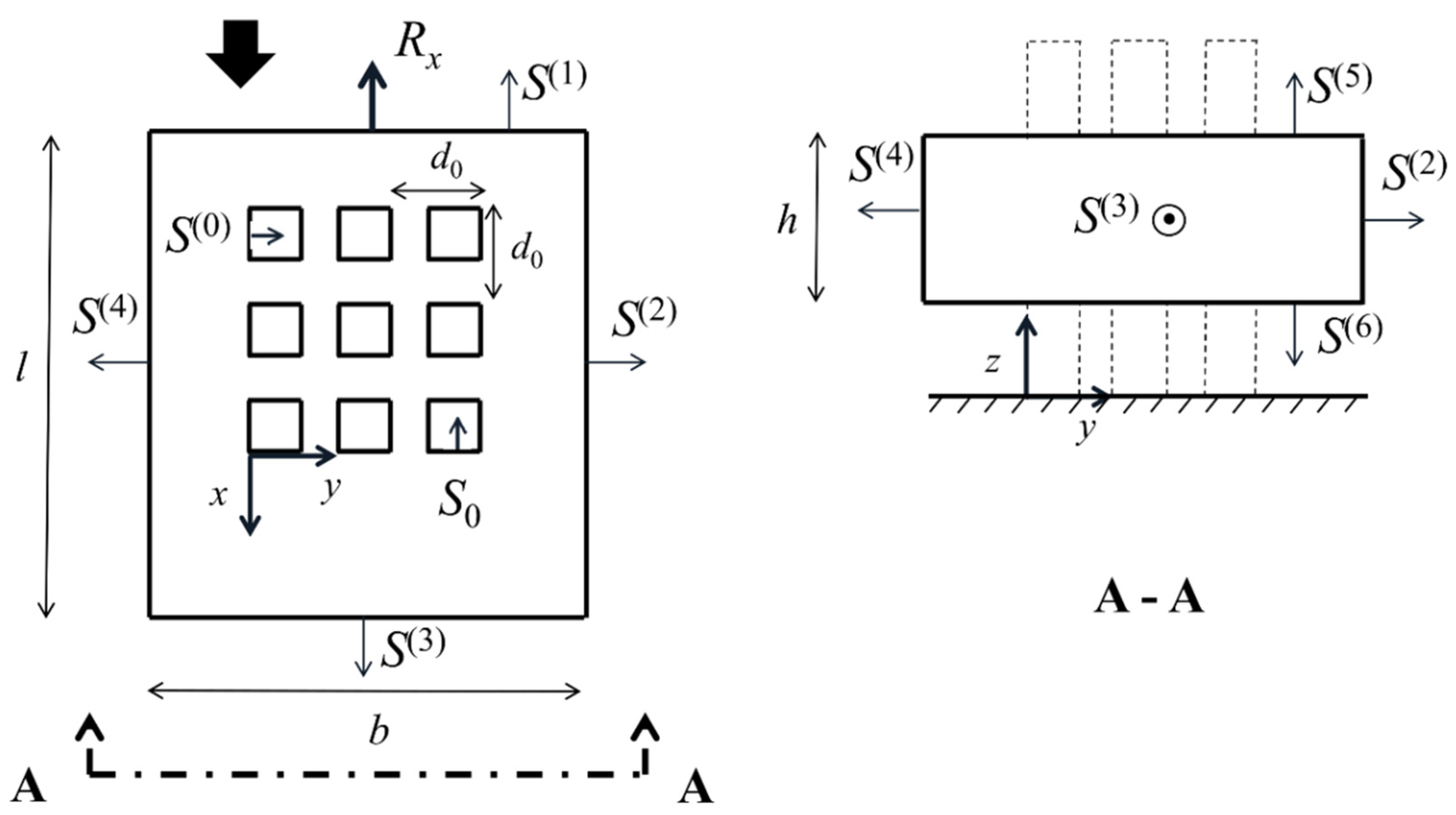
A control volume analysis is employed to compute the bulk drag force—the drag force on the totality of the cylinders in the array. The fluid control volume, shown in Figure 1, is limited by outer, open sections (sections S1 to S6), and inner, solid, sections (S0). There are momentum fluxes across the open sections. The forces applied on S0 constitute the reaction of the solid elements on the fluid in the control volume.
For a statistically stationary turbulent flow, the Reynolds-averaged integral equations of conservation of linear momentum (derived in the Appendix A and herein referred to as RAIM equations) are applied to the fluid control volume of Figure 1. Employing the Einstein-summation convention, they can be written:
where the free index i = 1, 2, 3 stands for the Cartesian spatial directions, Ui is the ith component of the time-averaged velocity vector, is the ith component of the velocity fluctuations, gi is the ith components of the acceleration due to gravity, P is the time-averaged pressure, ρ is the density of the fluid, Tik is the time-averaged viscous stress tensor and is the Reynolds stress tensor. The control volume is represented by Vc while Sc is the total control surface (the union of S1 to S6 and S0), S0 is the solid part of Sc, that coincides with the surface of the cylinders, and Sc\S0 represents the open control surface (the union of S1, …, S6), through which there may be mass and momentum fluxes. The components of the outward pointing normal unit-vectors applied to each boundary are ni. For the sake of conciseness, Equation (1) is written in Cartesian tensor notation, where the dummy index k is used in the summations inherent to the dot products in the first, fourth, fifth and seventh terms. The last two terms on the right-hand side of Equation (1) represent the force exerted on the flow by the cylinders:
where is the net pressure force and is the net viscous force.
If Equation (1) is applied in the streamwise direction, force Rx is the reciprocal of the bulk drag force applied on the cylinder array (FD), i.e., Rx = −FD and Rx = |Rx| = |FD|.
Point-wise time-averaged variables were weight-averaged in the corresponding control sections (accounting for the area of influence of each point) to calculate the integrals in Equation (1), i.e., , where Sm is an open control section, a(m) is a generic time-averaged variable measured in that control section, [ ] is the section-average operator, [a(m)] is the mean value of a in that section and S(m) is the area of the control section. Viscous stresses at the open boundaries of the control volume were considered negligible in comparison to Reynolds stresses. Resolving the integral terms, Equation (1) may be written as:
where θ is the angle between the channel bottom and a horizontal plane. If the thickness of the control volume h (Figure 1) is small compared to the other dimensions of the control volume, implying that the net mean momentum exchange in the vertical direction is negligible, then the last two terms on the right-hand side of Equation (3) may be omitted from the conservation equation:
The component Rx is estimated after all other terms in Equation (4) are determined experimentally, through acquisition of the three-component instantaneous velocity of the fluid in all open control sections and the free-surface elevation along the outer rim of the control section. If the vertical distribution of pressure is approximately hydrostatic, the calculation of the mean pressure on the surfaces is trivial and the gradients of the free-surface elevation are sufficient for the calculation of the pressure forces. Selecting a very thin prismatic control volume with its main dimension oriented parallel with the channel bottom, placed at an adequate distance above it, so that the effect of the bottom boundary to vertical distribution of velocities is not relevant, allows also for the definition of a single Reynolds number of reference for the assessed drag force [34]. The details of the mathematical derivation of Equation (3) are shown in the Appendix A.
2.2. Drag Coefficient
The drag coefficient of an isolated square cylinder, Cd, is expressed as:
where is the absolute value of the bulk drag force, h is the thickness of the control volume, d is the width of the square cylinder and U0 is the time-averaged longitudinal velocity that characterizes the undisturbed upstream flow, calculated as a spanwise average within the frontal area of the cylinder.
For the case of an array that consists of finite number of identical cylinders, the array-averaged Cd is defined as the normalised bulk drag force (Rx) averaged over the total number of cylinders (nc):
where is stagnation pressure, is a reference velocity representing the undisturbed flow upstream the array and defined as the longitudinal velocity laterally-averaged over the span of the cylinder array, and where is the exposed area of each cylinder.
3. Experimental Facility, Instrumentation and Experimental Procedure
3.1. Experimental Facility
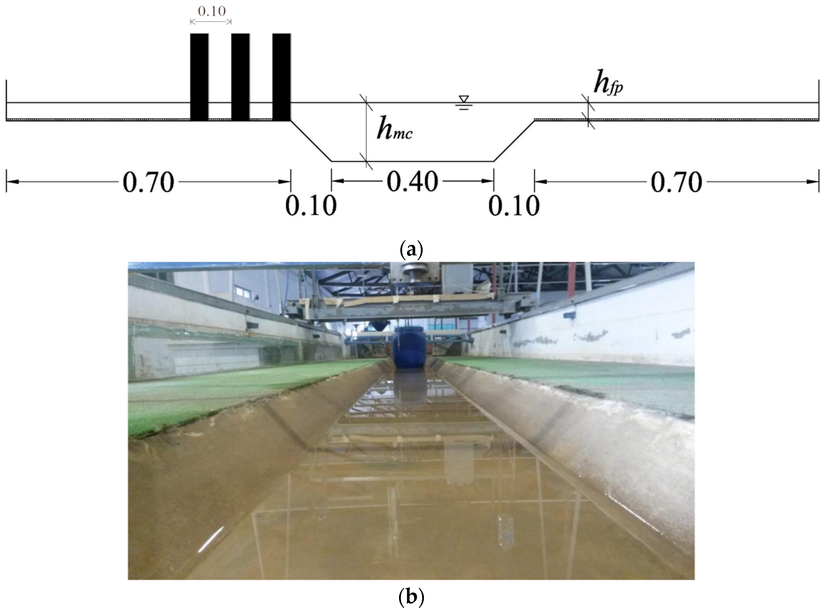
The experimental tests were conducted in the 10 m long prismatic and symmetric compound channel at the National Laboratory for Civil Engineering in Portugal (LNEC). The cross-section of the main channel is trapezoidal, while that of the floodplain is rectangular. The height of the main channel is 0.10 m and the slope of the margins (V:H) is 1.0. The exact dimensions are shown in Figure 2.
The bottom of the main channel is coated with polished concrete (hydraulically smooth). The floodplain is covered by a layer of synthetic grass, as described in [26]. The longitudinal slope of the channel is 0.0011. The inflow rates in the main channel and in the floodplain are regulated independently in order to achieve uniform-flow conditions at a relatively small distances from the entrance of the flow [37].
To minimize vertical accelerations and large-scale fluctuating motions, the flow is directed to the compound channel through a wall of perforated bricks in a tranquilization chamber and barrier of 0.02 m diameter PVC tubes. Acetate sheets are fixed at the end of the tubes pile for further tranquilization of the free surface. The flow depth at the outlet is controlled with tailgates, allowing uniform-flow depth for a given total discharge to be established. The channel is fed through a closed-circuit system involving a lower reservoir that collects the outflow of the channel, a stable-level upper reservoir that discharges into the channel and a pump station that connects the two reservoirs. The circuit ensures steady water head and discharge. Flow depth is measured by point gauges at 1.00 m and 8.00 m downstream of the channel entrance. The inflow rates in the main channel and the floodplain are monitored by electromagnetic flowmeters. A detailed description of the facility can be found in [38].
3.2. Experimental Tests
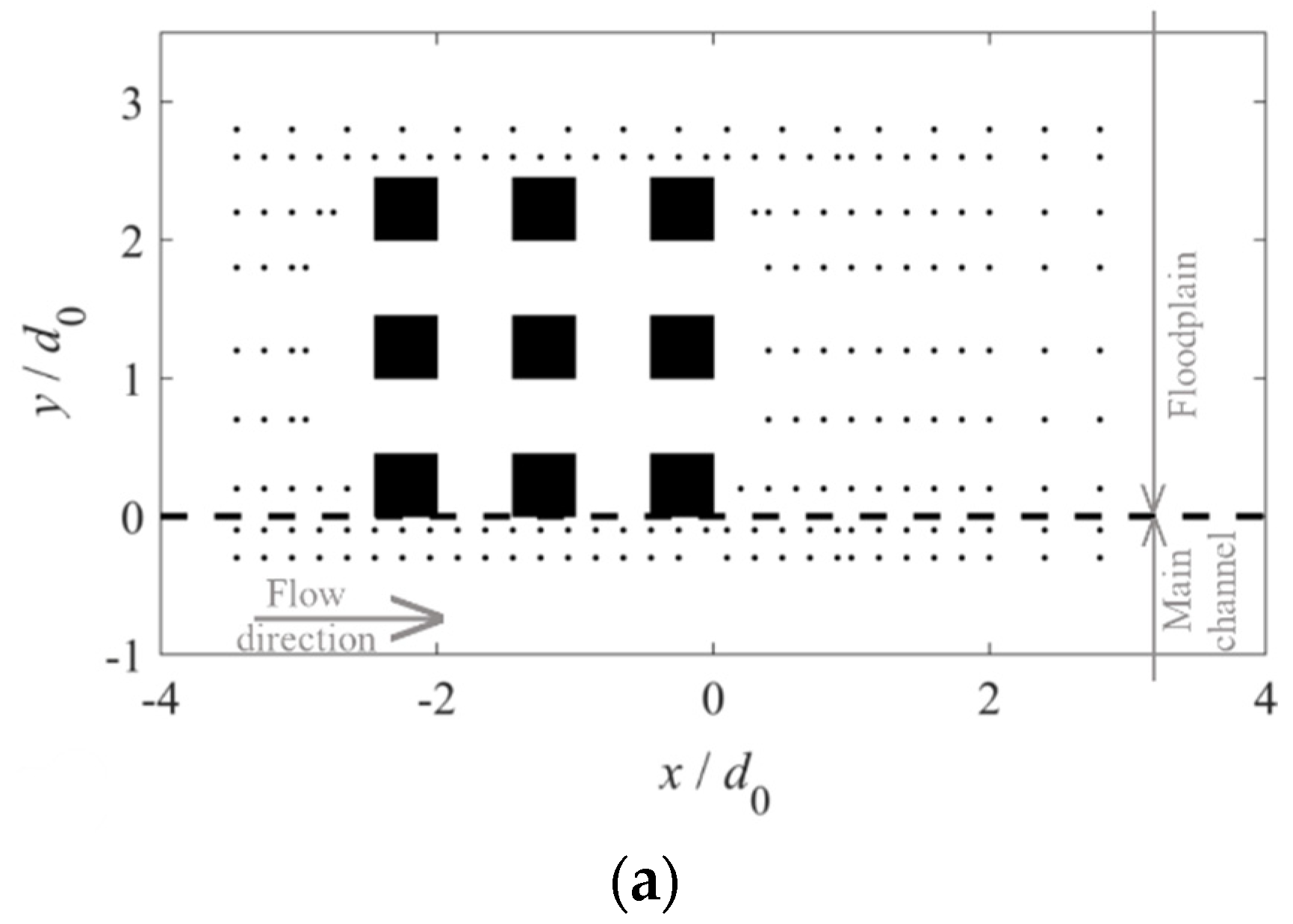
The experimental array is composed of nine square cylinders with width d = 0.045 m. It was placed at the interface between the main-channel and the flood plain, forming a grid orthogonal to the channel axis, as depicted in Figure 3. The distance d0 between two consecutive cylinders was kept equal to 0.10 m. Spacing and sizing were chosen so as to align with those of the experiments carried out in the context of FlowRes ANR, a project oriented to the investigation of compound-channel flows with transition in bed roughness, described in [39]. The tests were run under uniform-flow conditions in the compound channel. To establish uniform flow in the channel, the total discharge Q was initially distributed in the main channel (Qmc) and in the floodplain (Qfp), according to the weighted divided channel method proposed by [40]. The cylinders were emergent under the tested flow conditions.
Two tests were conducted, with different characteristics of the mixing layer. A summary of the flow parameters for both tests, named SA_03 and SA_04, can be consulted in Table 1. These include the Froude number (Fr) and the cylinder Reynolds number defined as Red = dU0/v, where is the kinematic viscosity of the fluid. The Froude number characterizes separately the main channel and the floodplain, and is given by Frfp = (Qfp/(1.40hfp))/√ghfp and Frmc = {Qmc/((0.40 + 0.20)(hmc − 0.10) + 0.05)}/√ghmc. The relative flow depth hr is defined as the ratio between the floodplain flow-depth hfp and the main-channel flow depth hmc. The normalized velocity difference is λ = (Umc − Ufp)/(Umc + Ufp) [27], where Umc and Ufp are the time-averaged and depth-averaged longitudinal velocities of the flow in the main channel and in the floodplain, respectively. In both flows, λ = 0.35, which indicates that the mixing processes should be dominated by two-dimensional planar interactions, associated to large-scale structures akin to Kelvin-Helmholtz instabilities. However, given that the value of λ is not significantly higher than 0.3, it was expected that three-dimensional effects in the mixing layer would not be negligible.
3.3. Velocity Measurements
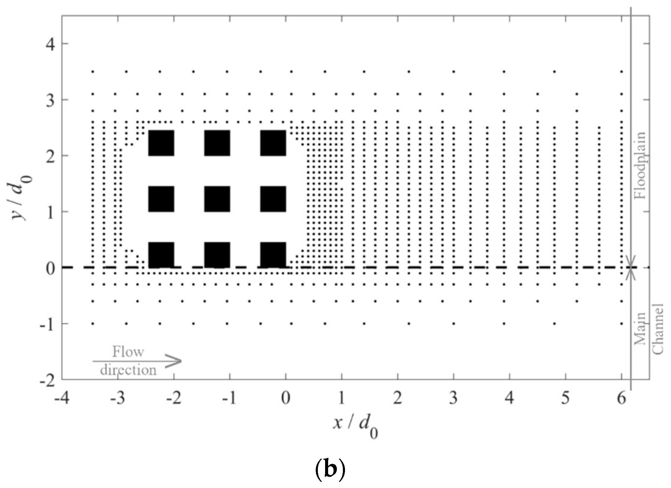
Time series of the three components of the instantaneous velocity were acquired simultaneously with a side-looking Nortek Vectrino ADV at a rate of 200 Hz. The sampling interval was 3 minutes and sampling locations are shown as grid points in Figure 3a (test SA_03) and Figure 3b (test SA_04). The grid is denser in the case of SA_04 to account for possible higher flow complexity due to more pronounced three-dimensional effects. The grid in both tests was applied at a distance z0 = hfp/3 from the floodplain bed and at z = hfp/3 − 0.06hfp.
Post-processing involved de-spiking with the phase-space filter proposed by [41]. Time-series that exhibited bad data in more than 60% of their initial number of samples were eliminated. Time-averaged results of the corresponding grid points were replaced by space-interpolated values. These points represent less than 7% of the total number of grid points and are confined to the region close to the cylinders’ walls.
Free-surface time-series were acquired with ultrasonic distance-measuring sensors at a rate of 10 Hz during 2 min. These measurements were taken in the points of the grid that correspond to the outer rim of the control volume. The free-surface recordings were transformed into hydrostatic pressure forces at sections S1 to S4.
4. Results
4.1. Time-Averaged Flow and Main Wake Processes
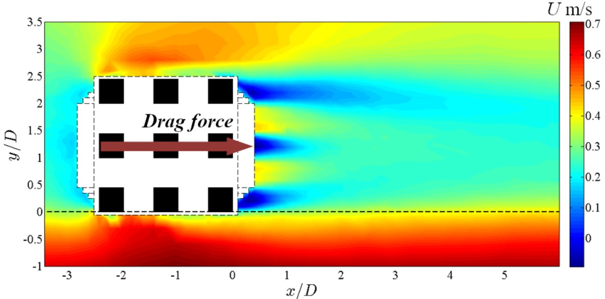
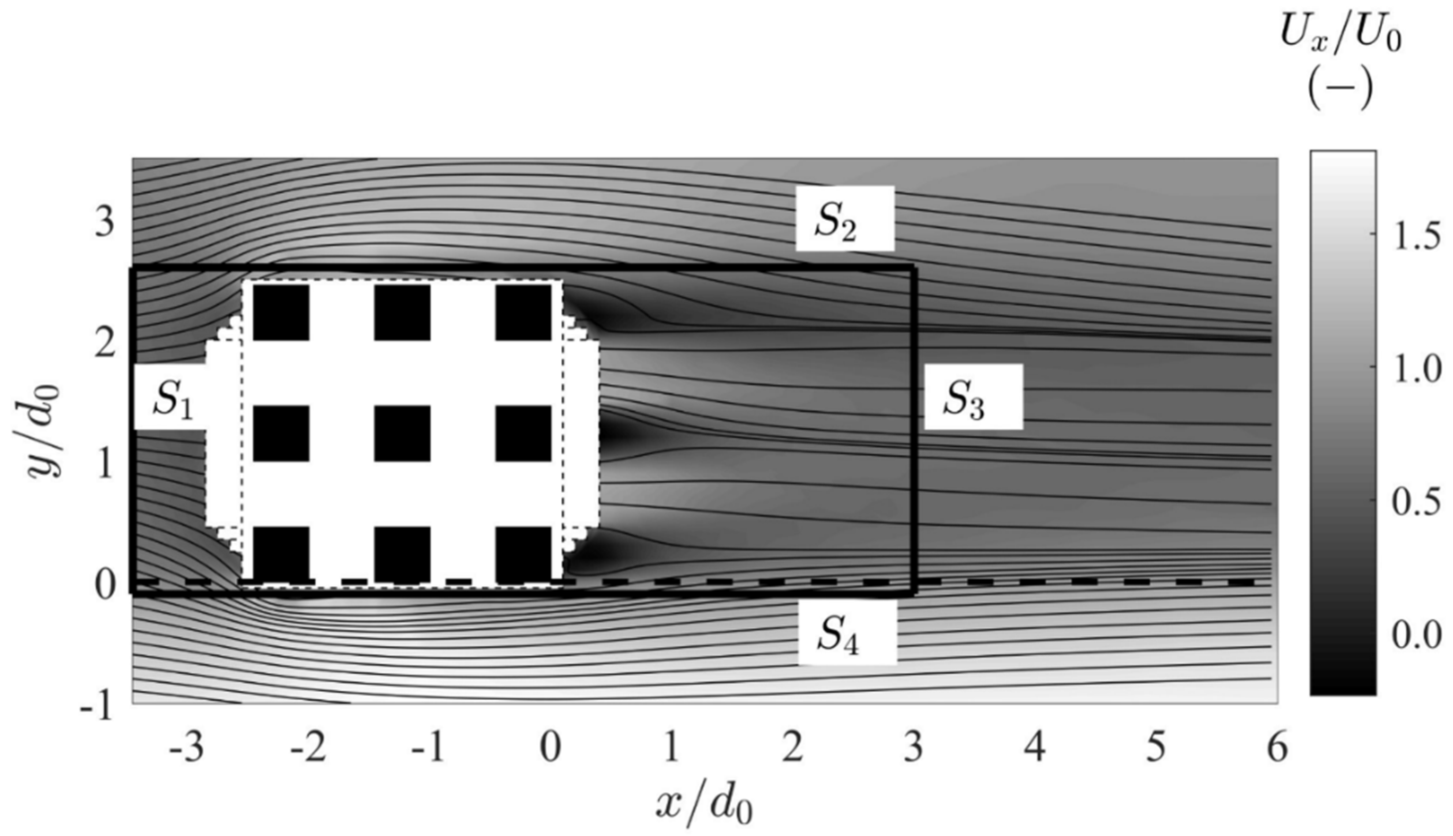
The streamlines and the spatial distribution of the absolute value of time-averaged streamwise velocity are shown in Figure 4 for the SA_04 test. The control volume encompasses the near-wake field [42] of the array, where intense momentum exchange and turbulence occur. The spatial distribution of the velocities is indicative of the main wake-flow processes in both tests since similar patterns were also observed in the SA_03 test.
The ratio (d0−d)/d of the array is equal to 1.22, a value similar to that for which [13] described the relevant wake patterns as the “gap-flow mode”. This wake flow features an alternatively deflecting jet along the streamwise direction between the cylinders and a nested vortex-shedding process within the one formed by the outward edges of two side-by-side cylinders. The streamlines observed in Figure 4 are compatible with this pattern with one notable exception—the formation length of the cylinder adjacent to the interface is smaller than that of the cylinder placed towards the floodplain. This indicates that drag is unevenly distributed in the lateral direction. The observed high velocities of the flow in the near wake and the relative small formation length of all downstream cylinders may indicate limited downstream velocity-deficits and, in turn, decreased bulk drag compared to that on an array with (d0−d)/d >> 1.5 [13].
The patterns of the streamlines denote the main changes in the flow direction as it passes through the array. Upstream of the array, flow deflection at the frontal area of the cylinders is obvious. The deflected streamlines are directed both towards the main channel and the inner floodplain. The latter direction though, seems to present higher angles with the upstream-flow direction and the effect is traceable within a greater region in the floodplain (Figure 4). This may be attributed to the significantly lower flow velocities in the floodplain than those in the main channel, allowing the occurrence of greater yaw angles [43]. Downstream of the array the flow is attracted by the low-pressure region formed at the shaded areas (the formation length). Again, streamline angles with the main-flow directions in the floodplain are greater than the respective ones in the main channel, illustrating the effects of the time-averaged shear flow.
4.2. Analysis of Terms in Equation (4)
The terms of Equation (3) were calculated for a control volume with b = 2.7d0, l = 6.25d0 (note that the plan view of the control volume also shown in Figure 4) and h = 0.06hfp. The momentum fluxes and the Reynolds stresses computed from the velocity measurements at z0 = hfp/3 (section S5) and z = hfp/3−0.06hfp (section S6) confirmed that net momentum flux across sections S5 and S6 is negligible and that the vertical variation of the turbulent stresses is small, justifying the application of Equation (4). All values are normalized with powers of the reference velocity U0 estimated for each test. The values of the terms of Equation (4) are shown in Figure 5, Figure 6 and Figure 7.
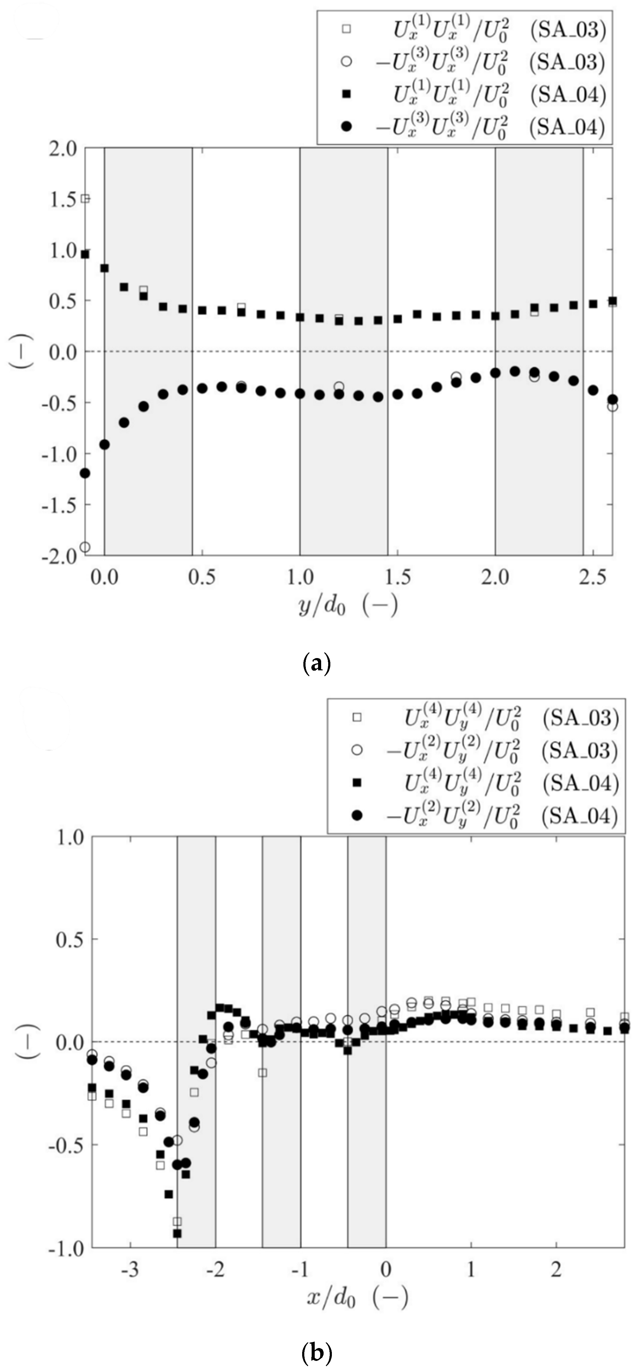
The mechanisms underlying the intense increasing of the curvature of the streamlines involve momentum transport. The distributions of the convective transport UxUk at the vertical control sections S1, S2, S3, S4 are presented in Figure 6a,b. The product UxUk is also called as mean flux, as it represents the momentum flux of the time-averaged flow per unit mass and area, transported in the streamwise direction. The signs of the terms are chosen so that they represent simple summations in Equation (4).
As shown in Figure 5a, the maximum values of mean fluxes, in both control sections S1 and S3, are observed near the main-channel/floodplain interface, as a consequence of the higher velocities in the main channel. For the chosen locations of S1 and S3, both tests present rather balanced fluxes and a near zero net momentum flux. This was sought as a compromise, since placing the S1 and S3 very near the cylinder array would increase the uncertainty in all measured variables. This is especially true for the free-surface at S3, because of the stronger vertical fluctuations generated by the interaction of the cylinder wakes and the lateral fluxes between the floodplain and the main channel.
Momentum transport along the lateral surfaces of the control volume S2 and S4 for both tests is shown in Figure 5b. Flow deflection upstream the array (out of the control volume-negative values in Figure 5b), observed in Figure 4, is also discernible here. The maximum values of the convective transport through these sections occurs just upstream the cylinder array. Flow reattachment is observed downstream the array. In both tests it seems that mean momentum transport out of the control volume upstream the array is higher close to the main channel (S4) than in the inner floodplain (S2). The different characteristics of the mixing layers of tests SA_03 and SA_04 is visible in the different values of the convective transport downstream the first row of cylinders. The outward convective fluxes upstream the cylinder are not influenced by the nature of the mixing layer. However, beyond the first cylinder row, the convective flux near the interface , oscillates between positive (inward in this context) and negative (outward) values. This is especially visible in the higher submersion test SA_04. The negative fluxes are much less expressive in the second and third rows, relative to those upstream of the first row. Outward convective fluxes are not seen at boundary , next to the floodplain. This may indicate a perturbation in the array induced by the flow in the main-channel.
Note that the array spacing ratio is d0/d = 2.22, compatible with the range 1.5 < d0/d < 4 proposed by [12] for partially reattaching flow between two consecutive cylinders. Yet, the flow pattern and the convective fluxes at the boundary seem to indicate that the boundary layer separated from the upstream cylinder does not reattach to the side of the downstream cylinder but is driven inwards in the space between these two consecutive cylinders. It can be hypothesized that the relevant variables are the momentum difference between the main channel and flow in front of the array of cylinders and the space between the cylinders. In that case, a Reynolds number can be formed, . Test SA_03 (lower submergence) is characterized by while SA_04 (higher submergence) has .
The perturbation imposed by the flow at the interface on the flow in the space between cylinders should be mainly a reduction of the pressure difference across the first cylinder, similar to what is found in arrays affected by cross-flow [20]. On the second and third cylinders, the effects of the perturbation are more difficult to envisage: for instance, while lateral intrusion of momentum may contribute to increase the pressure downstream the second cylinder, it may also increase the pressure upstream that cylinder, which, in the reattachment regime, could be lower than the downstream pressure. In the absence of data to clarify this issue, it is further hypothesized that the overall effect of the perturbation induced by the flow at the interface on the flow in the space between the cylinders is to lower bulk drag force. It follows that the higher the value of , the larger the perturbation and the lower the normalized drag force. Test SA_04, with the higher submergence and the higher momentum at the interface, should be the most affected.
On the side of the floodplain, section , the regularity of the convective fluxes is compatible with cylinders in the reattachment regime characterized by none-to-weak vortex formation and negative drag acting on the downstream cylinder. The occurrence of negative drag is highly probable in the last row, which was also observed by [14] for d0/d < 3 and Red~5600–12,800.
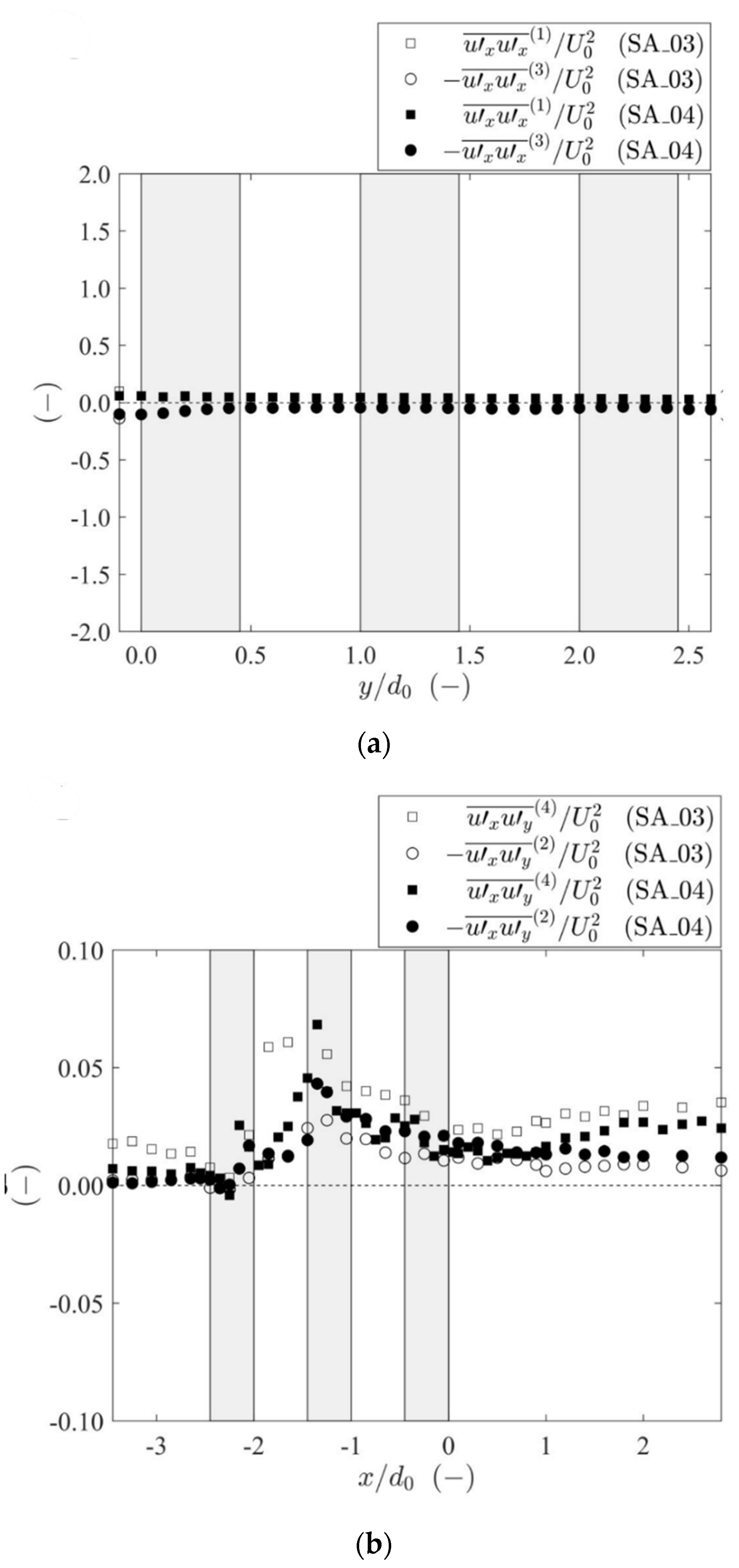
The values of the turbulent transport , normalized with the scale velocity U0, are shown in Figure 6a,b. The variable is also referred as stress, since it expresses the Reynolds stress per unit fluid density. The values of the stresses, both normal and shear, are smaller than those of the convective fluxes. This observation is highlighted by the use of the same scale of the vertical axis in Figure 5a and Figure 6a. The stress values in S1 and S3 (Figure 6a) resemble the distribution of the streamwise convective momentum transport (Figure 5a) featuring higher values at the main-channel/floodplain. Stronger stresses near the interface (y/d0 = 0) are typical of compound-channel flows [23], which suggests that these peaks are not due to the presence of the array. The corresponding peak for S3 is larger in both tests, compared to that of S1. This observation implies that there is an excess in the stress, generated by interaction of the wake flow in the near-interface cylinder and the shear flow. This effect seems more pronounced in the case of test SA_03–lower submersion.
The shear stresses on the lateral control sections S2 and S4 are seen in Figure 6b. It is noteworthy that the peak values are obtained at the second row of the array, following a turbulence suppression caused by the accelerated flow upstream the first row. It is also relevant to note that in the case of test SA_03 (lower submergence) turbulent transport is much higher on the side of the interface (S4). In the case SA_04 (higher submergence), turbulent transport is higher in section S4, relatively to section S2, just upstream the second row and for onwards. Downstream the latter section the characteristics of the compound flow mixing layer become again prevalent, relative to those of the array wake flow. In the space between the first and the second rows, the separated boundary layer from the first cylinder may seem to cross the section, in the case of test SA_03. However, this is not the case of SA_04, which is line with the hypothesis that, for this test, boundary layer reattachment occurs inside the space between cylinders (see discussion of convective fluxes at ). This justifies the stronger difference between shear stresses at and at , in case of SA_03.
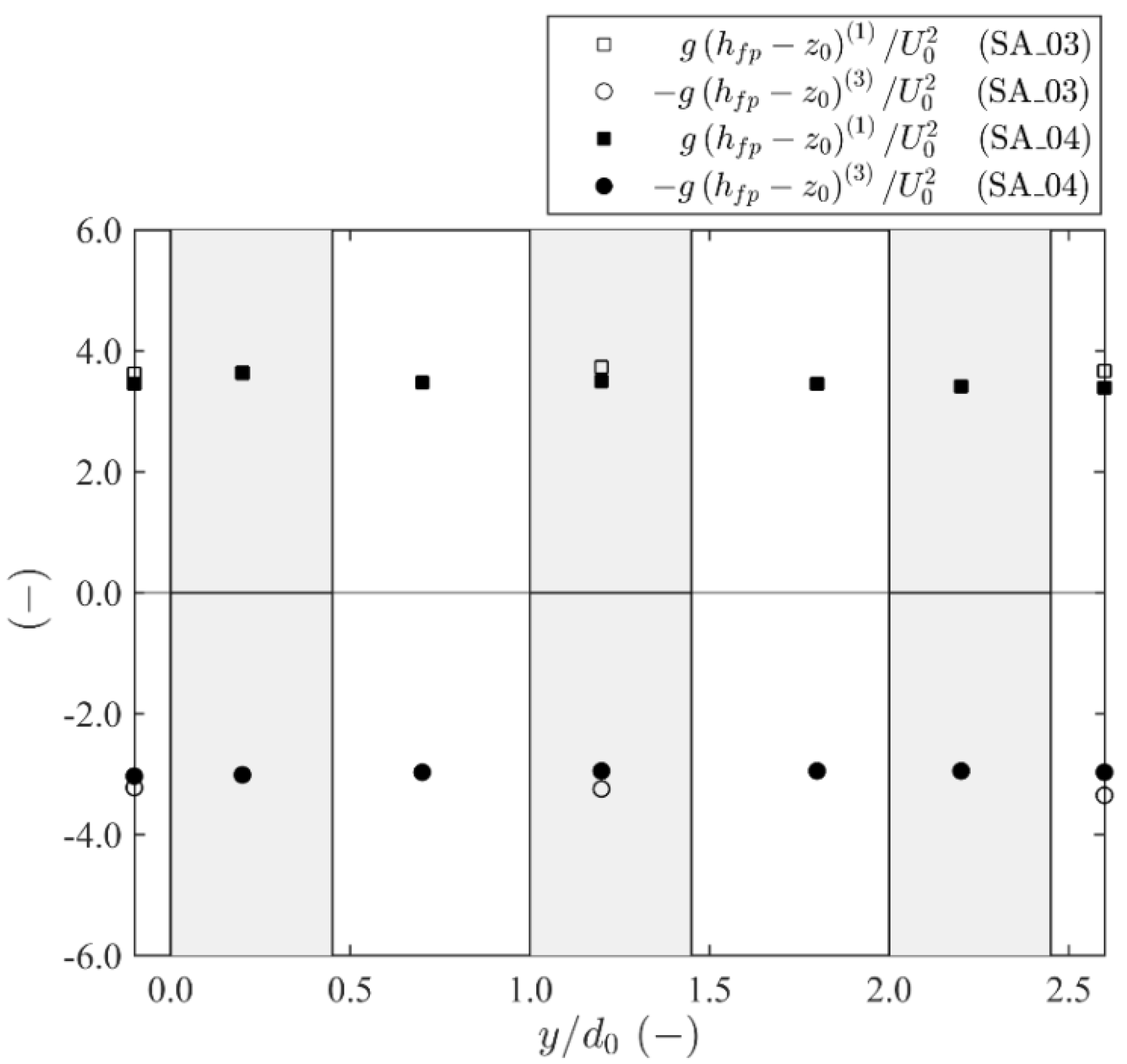
The distribution of the terms , proxies for the pressure forces in Equation (4), assumed hydrostatic, are shown in Figure 7. Pressures upstream the array are larger than pressures downstream. It is recalled that the convective momentum flux measurements shown in Figure 5a revealed a very small imbalance between incoming (at ) and outgoing () convective momentum fluxes.
Lateral net later flux of momentum mostly compensates for the longitudinal momentum lost due to deflection in front of the array. However, the irreversible loss of mechanical energy in the fluid–cylinder interactions results in the pressure drop visible in Figure 7.
4.3. Total Net Contribution of Terms in Equation (4)
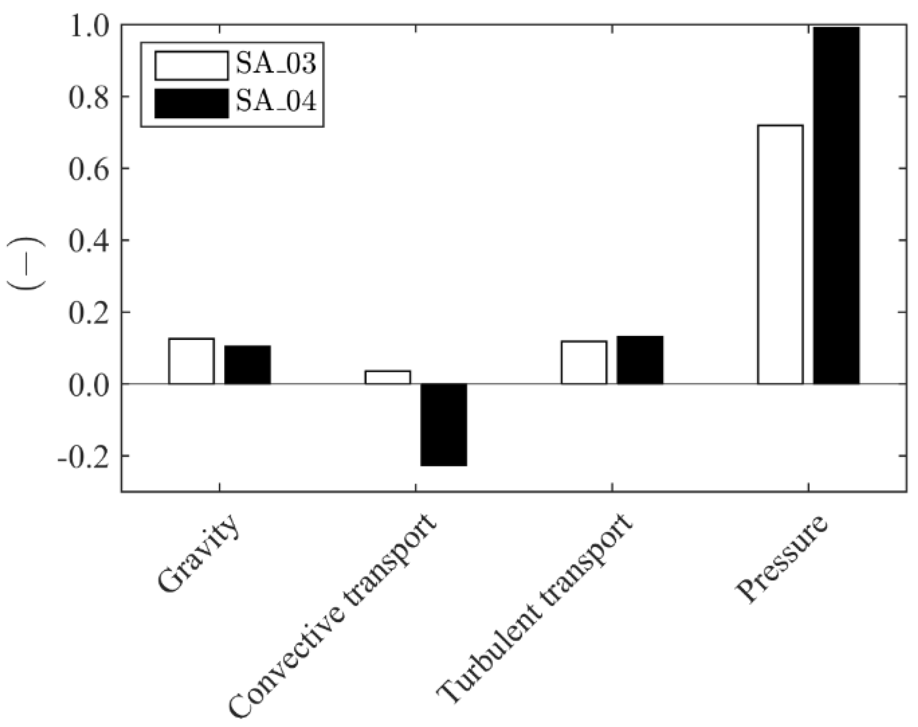
The net contributions of the terms of Equation (4) for both tests referring to the fluid control-volume of Figure 4 are quantified and presented in Figure 8 as percentages of the absolute value of the drag force.
The term is referred to as net convective transport, the term is referred to as the net turbulent transport, the term as the pressure imbalance and the term as the gravity contribution. Figure 8 shows that the pressure imbalance between S1 and S3 is the single major contribution for the drag force. This raises concerns about the accuracy of the estimation of the drag coefficient, given the assumption of the hydrostatic hypothesis.
While the pressure drop is the dominant term, it is also clear that the effects of the mixing layer, expressed through the contributions of the net convective transport and the net turbulent transport, cannot be neglected. The different contributions of the net convective transport of SA_03 and SA_04 justify quantitative and qualitative differences in the value of the drag coefficient.
The negative value of the net convective transport can be seen as an effect of the higher momentum imbalance between the flow in the main-channel adjacent to the interface and the flow in front of the array. The physical processes involved were presented in Section 4.1. It is hypothesized that the penetration of flow from the main channel into the space between cylinders contributes to reduce the pressure imbalance, particularly in the first cylinder row. The main attribute of this penetration is to reduce the value of the net convective momentum transport.
Finally, it should be underlined that the net turbulent momentum transport is not negligible, even if the fluxes associated to Reynolds stresses are one order of magnitude smaller than convective fluxes. Failure to include the turbulence contributions would result in errors of 10% to 15% in the value of the drag coefficient.
4.4. Sensitivity Analysis of the Values of the Drag Coefficient Relatively to the Position of Section S3
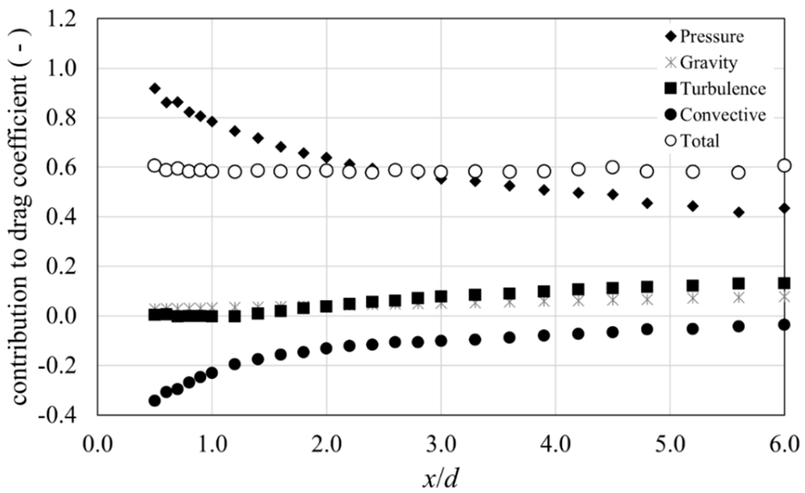
Mean flow and turbulence at the wake of the array are seen to strongly vary longitudinally. To demonstrate the validity of the present integral method, it is necessary to assess the sensitivity of the values of the drag force and of drag coefficient to the changes in the wake flow. The drag coefficient was computed for different control volumes, differing only in the longitudinal positions of section and, hence, of length l (Figure 1). The bulk drag force on the array of cylinders was estimated according to Equation (4) and the drag coefficient was computed from Equation (6).
The different net contributions for the different control volumes are shown in Figure 9, for the case of test SA_04, for which the density of measurements was higher. Each contribution corresponds to its array-averaged value divided by the reference stagnation pressure and by the exposed cylinder area . As an example, the pressure contribution corresponds to . The simple sum of all the contributions is the value of the drag coefficient. It is verified that the values of the drag coefficient are not significantly sensitive to the location of the downstream boundary. As examples, the values of the drag coefficient for , and are 0.583, 0.578 and 0.580, respectively.
If the boundary is placed very near the cylinder array, the pressure imbalance is larger, but the negative contribution of the net convective transport is also larger. These negative values express the negative contribution of the outward momentum fluxes in the upstream reaches of the control volume, which, for short lengths, are not balanced by the positive inward contributions in the wake. As the length of the control volume increases, the positive momentum (inward) contributions increase, and the net momentum transport becomes less negative. Evidently, the further the section is placed, the smaller the pressure imbalance. The net turbulent transport increases with the length of the control volume as it picks up the lateral shear stress imbalance between the interface and the floodplain, downstream of the array.
4.5. Values of the Drag Coefficient and Discussion
The array-averaged values of Cd for tests SA_03 and SA_04 are presented in Table 2. The same table summarizes the values of drag coefficients found in other studies, corresponding to different configurations of square cylinders and types of flow. Among these, some employ cylinders in open-channel flows [23], closed water-channel flows [44] and air flows [13]. One case concerns a regular array in open-channel flow [23] and the others regard cylinder pairs arranged in tandem or side-by-side configurations with relative distance between the cylinders d0/d similar to that of the regular array examined herein. All Cd values in Table 2 are array-average values. As a general trend, the drag coefficient of square cylinders in tandem is smaller than that of isolated cylinders in uniform flow. The drag coefficient of cylinders in a side-by-side configuration may be increased relatively to that of isolated cylinders. The drag coefficients of the tests conducted here (SA_03 and SA_04) are smaller than those of isolated cylinders and also smaller than those of cylinders in tandem for the same cylinder spacing and range of Reynolds number. The larger cylinder spacing reported by [12] features lower values of the drag coefficient. This is attributed to the lower value of the Reynolds number and not discussed in this paper. The discussion below addresses the reason why the drag coefficient of the cylinders in the mixing layer is smaller than that of cylinders in tandem in uniform flow and clarifies the differences between the values obtained for the two tests SA_03 and SA_04.
Test SA_03, with the lower relative submergence, yielded the higher drag coefficient. The different values of the drag coefficient are mainly due to the differences in the net convective transport. Without this term, the summation of the normalized contributions for the drag coefficient are 0.72, for test SA_03, and 0.70 for test SA_04. The different values of the net convective transport express different hydrodynamics of the interaction between the compound channel mixing layers and the flow within the array.
It hypothesized that the key difference between test SA_03 and SA_04 is a result of the difference between the momentum in the main channel and the momentum of the flow in front of the array. If this difference is normalized by the total momentum transported compound channel, one obtains a parameter that is approximately the same as the normalized shear rate. This parameter is fundamental to understand the nature of the mixing processes between floodplain and main channel in the absence of localized perturbations. In the presence of the finite array, it is hypothesized that it is not appropriate to scale the momentum difference by any other momentum quantity, since the array locally disrupts the lateral exchange processes of the compound channel flow. Instead, it is proposed that the momentum difference between the flow in the main channel and the flow in front of the array should be taken as a measure of the ability of the flow in the main channel to penetrate in the space between consecutive cylinders. The velocity difference, a geometrical variable expressing the distance between consecutive cylinders and the fluid properties density and viscosity are grouped into a Reynolds number that may be more adequate to parameterize the differences in the net convective transport.
The differences between test SA_03 and test SA_04 are thus not a simple consequence of different relative submersions of the floodplain. The latter are a result of different discharges in the main-channel and in the floodplain. The higher momentum transported in the main-channel in test SA_04 (with the higher relative submersion) induces a change in the reattachment regime of the cylinders adjacent to the floodplain relatively to what would be expected in a simple array in uniform flow. This change, envisaged in the values of the momentum fluxes at section and in the pattern of streamlines shows, consists in a deflection of the separated boundary layers from the upstream cylinders. As per the effect of lateral momentum influxes, they do not re-attach at the outer walls of the downstream cylinders, as is expected in that range of Reynolds numbers and cylinder distances, but against the upstream faces of the downstream cylinders.
It is noteworthy that both tests produced significantly smaller values of Cd, comparatively to those of isolated, tandem or side-by-side cylinders in uniform flows (see Table 2). The array-averaged values of Cd of both SA_03 and SA_04 are closer to those of tandem cylinders than to those of the side-by-side reported by [14] or [13] for the same ranges of the Reynolds number and of the ratio d0/d. It is thus hypothesized that downstream cylinders, especially those on the inner column or on the side of the floodplain, experience significantly less drag—or even negative drag—than that of the upstream cylinder. In short, it was expected that the array-averaged drag coefficient of the array under investigation would be smaller than that of an isolated cylinder, since each column is likely to behave as a system of cylinders in tandem, even if the side-by-side configuration may attenuate this effect. The additional drag reduction brought about by the mixing layer called for an explanation. It was hypothesized that it should be the effect of convective fluxes that equalize pressures across the second row of cylinders, especially in the column adjacent to the interface, an effect that is stronger in test SA_04.
It was earlier argued that the relative importance of the pressure forces to the total drag force poses the question of the accuracy of the results, given the hydrostatic hypothesis. Deviations from hydrostatic pressure distribution are expected only if streamlines exhibit strong vertical curvatures. It is unlikely that such strong curvatures are found in this flow. In the case of the upstream section, the values agree well with those obtained by application of the Bernoulli principle—conversion of kinetic head into pressure head. In the case of the downstream section, the results of Figure 9 show that the drag coefficient is essentially independent of the longitudinal position of that section. Given that vertical accelerations are more likely to occur just downstream of the array, it is concluded that streamline curvature in the vertical plane should be negligible everywhere.
As a last remark, concerning the precision of the results, if it is assumed that the precision of the free-surface measurements at the downstream section is 1 mm, the values of the drag coefficient would vary as follows: 0.742 ± 0.09, for test SA_03, and for test SA_04.
5. Conclusions
This study was aimed at experimentally assessing the bulk drag force on arrays of cylinders in compound channel mixing layers and the corresponding array-averaged drag coefficients. The drag force was estimated by applying the Reynolds-averaged integral momentum conservation equations (RAIM) in a fluid control-volume around the array. The robustness of the methodology was demonstrated by carrying out a sensitivity analysis to the size of the control volume. It was shown that the values of the drag coefficients do not depend on the location of the downstream section.
Two values of the relative submergence were tested. It was found that the values of the array-averaged drag coefficients, of both tests, are smaller than those of cylinders in tandem or side-by-side, obtained for comparable values of the Reynolds number and cylinder spacing. Drag reduction in the downstream cylinders of a tandem arrangement has been verified in the reattachment regime. The drag reduction observed in the tested arrays should be partially explained by a strong drop of the pressure imbalance in the downstream rows of the array, leading, possibly, to negative drag.
Further drag reduction should be due to the effect of lateral convective fluxes of momentum from the main-channel to the space between consecutive cylinders. This perturbation is likely to strongly reduce the pressure imbalance on the first cylinder row, on the side of the main channel. It is argued that this effect should become more pronounced with the increase of the difference between the momentum in the main-channel flow and the momentum of the flow in front of the array. The value of the array-averaged drag coefficient should thus be inversely proportional to a power of the Reynolds number . Test SA_04 featured the highest imbalance of momentum relatively to the kinematic scale and, hence, exhibited the stronger drag reduction. The normalized shear rate or the relative submergence, per se, are not adequate parameters to express drag reduction in cylinder arrays in the mixing layer of compound channel flows. Further attention should be given to finding a relation between the variation of the drag coefficient of finite arrays in mixing layers with for a wider range of normalized shear rates, Reynolds numbers and relative floodplain submersions.
This study is meant to provide researchers on urban flooding with a conceptual framework to derive drag forces from fundamental principles of hydrodynamics and to propose an actual quantification of drag coefficients susceptible to be used in simplified two-dimensional shallow-water models using, e.g., porosity approaches to determine momentum and energy losses due to urban meshes. The method used in this study provided values for the drag coefficient at a height of approximately 1/3 of the flow depth above the floodplain bed. In principle, the method can be applied to obtain depth-averaged estimates of the drag coefficient. For that purpose, it would be beneficial to obtain velocity data at several horizontal planes. The method is sensitive to the errors in the pressure forces. The assumption of hydrostatic vertical pressure distribution is an important limitation. The method can be improved if pressures are taken with pressure transducers. Another improvement would be the determination of all three velocity components in planar regions with stereo particle image velocimetry. This would allow for the calculation of instantaneous forces on the cylinders provided that the velocity measurements could be synchronized with pressure acquisitions. It would thus strengthen the argument that the additional drag reduction due to the mixing layer is mainly the effect of the lateral convective fluxes that equalize pressures across the second and following rows of cylinders.
Author Contributions
Conceptualization, R.M.L.F. and A.M.R.; Data curation, E.A. and A.M.R.; Formal analysis, R.M.L.F., M.G. and A.M.R.; Funding acquisition, R.M.L.F.; Investigation, M.G. and A.M.R.; Methodology, R.M.L.F., P.P., E.A. and A.M.R.; Project administration, R.M.L.F.; Resources, E.A.; Supervision, R.M.L.F., P.P. and E.A.; Writing—original draft, M.G.; Writing—review & editing, R.M.L.F. and A.M.R. All authors have read and agreed to the published version of the manuscript.
Funding
The second author was funded by the Marie Curie FP7-PEOPLE-2013-ITN program of the European Union, through the SEDITRANS project. Other aspects of the research were funded by FEDER-COMPETE2020 (POCI) and Portuguese funds (Foundation for Science and Technology, IP) through project PTDC/ECI-EGS/29835/2017-ASHES.
Informed Consent Statement
Not applicable.
Acknowledgments
The current experimental work was aligned with the objectives of the FlowRes ANR Project (2015–2018), IRSTEA, towards characterization of compound-channel flow, influenced by various floodplain land-uses.
Conflicts of Interest
The authors declare no conflict of interest.
Nomenclature
The following symbols are used in this paper:
| α | generic time-averaged variable; |
| b | width of the fluid control-volume; |
| C | forces-normalization quantity; |
| Cd | drag coefficient; |
| d | width of square cylinder; |
| d0 | distance between two consecutive cylinders; |
| Fr | Froude number; |
| FD | time-averaged force exerted by the flow on the cylinders; |
| g | gravitational acceleration; |
| h | height of the fluid control-volume; |
| hr | relative flow depth in a compound channel; |
| K | shear parameter; |
| l | length of the fluid control-volume; |
| n | outward pointing normal unit-vector; |
| nc | number of cylinders of an array; |
| P | time-averaged pressure of fluid; |
| Q | discharge in the channel; |
| Red | Reynolds number based on cylinder’s width; |
| Reynolds number based on the velocity difference between the flow in the main- channel and in the array and on the cylinder spacing; | |
| R | time-averaged force exerted by the cylinders on the flow; |
| Rx = |FD| | absolute value of the time-averaged drag force on the cylinders; |
| Sc | total surface of the fluid control-volume; |
| Sm | open control-section; |
| S(m) | area of an open control-section; |
| Tik | time-averaged viscous stress tensor; |
| t | Time; |
| U | time-averaged velocity; |
| U0 | mean representative velocity of the approaching flow to the cylinder array; |
| Reynolds-stress tensor; | |
| Vc | control volume; |
| z0 | vertical distance of the measuring level from the floodplain bed; |
| x, y, z | longitudinal, lateral and vertical directions; |
| θ | angle between the channel bottom and the horizontal plane; |
| λ | dimensionless shear; |
| ν | kinematic viscosity of fluid; and |
| ρ | density of fluid |
| Subscript or superscript m (m = 1, 2, 3, 4, 5, 6) refers to an open control-section | |
| Subscripts mc and fp refer to main channel and floodplain respectively | |
Appendix A
Reynolds transport theorem is applied to a fixed control volume containing an incompressible Newtonian fluid. The control volume is not simply connected, has open boundaries (allowing for mass fluxes across it) and closed boundaries (not allowing for mass fluxes), the latter representing the boundaries of solid objects. The integral equation of conservation of linear momentum thus obtained is:
where Einstein’s summation convention is expressed in the repetition of index k. In Equation (A1), the free index i assumes the values i = 1, 2, 3 for the three Cartesian directions. Time is identified by t, the ith component of the velocity vector is , the pressure is p, the fluid density is , the viscous stress tensor is and he acceleration due to gravity is . Since the fluid is incompressible , where is the viscosity of the fluid and the comma (,) stands for partial derivative. The boundaries of the control volume are denoted , in general. The closed boundaries are denoted and, hence, the open boundaries are denoted . For the purpose of this study, it is assumed that the closed boundaries express the outer boundary of a solid body on which hydrodynamic actions are to be evaluated. The components of the unit vector applied in each boundary and pointing outwards (from inside to outside the control volume) are denoted .
Reynolds decomposition involves expressing particular instances of velocities and pressure (for instance instantaneous values) as the sum of an ensemble average and a fluctuation: and (the capital letter stands for ensemble average and the prime stands for fluctuation). Introducing the Reynolds decomposition in Equation (A1), ensemble averaging, and restricting the application to statistically stationary flows, the Reynolds-averaged integral momentum (RAIM) conservation equations are obtained
where the overbar stands for ensemble-averaging and is the ensemble-averaged viscous stress tensor. In this stationary case, the ensemble average can be thought of as a time average. The analysis is further restricted to flows with sufficiently high values of the Reynolds number, so that the effects of the viscous tensor can be neglected in the interior of the control volume and in the open boundaries but not necessarily at the solid boundaries. Equation (A2) thus becomes:
This analysis is used to determine the hydrodynamic actions on the solid parts of the control boundaries. The reaction of the solid walls onto the fluid in the control volume is the integral:
The minus sign in definition (A4) is a matter of convention–it is assumed that the hydrodynamic action on the solids in the control volume, , is along the main flow direction and that the x-direction is aligned with this direction. Hence, given that , the reaction of the solids in the control volume is assumed to be against the direction of the main flow. Introducing these assumptions and definitions in Equation (A3), one obtains:
If Equation (A5) is applied to the control volume of Figure 1 and is solved for , (the component in the direction of the main flow) one obtains:
To improve readability, Einstein’s summation convention is kept in Equation (A5). However, instead of the x-direction is made explicit. The outcome of Equation (A6) is positive if the drag force is along the main flow direction.
The conversion of the integral terms in Equation (A5) to summations of discrete values, applying the trapezoidal rule, leads to:
where is the inclination angle of the channel. The area and the outward unit vectors of each section are denoted and , respectively. Variables and are the distributions of velocities and pressure, respectively, for each section m. The operator [ ] is the section-average operator such that [a(m)] is the mean value of a in that section. The unit vectors for the arrangement in Figure 1 are n (1) = (−1, 0, 0), n (2) = (0, +1, 0), n (3) = (+1, 0, 0), n (4) = (0, −1, 0), n (5) = (0, 0, +1), n (6) = (0, 0, −1). Applying the directions of the outward unit vectors, the operational equation for Rx is:
It is noted that the drag force on the cylinders is the reciprocal of vector R, in the x-direction i.e., and .
References
- Jain, V.; Fryiers, K.; Brierley, G. Where do floodplains begin? The role of total stream power and longitudinal profile form on floodplain initiation processes. GSA Bull. 2008, 120, 127–141. [Google Scholar] [CrossRef]
- Dieck, J.J.; Ruhser, J.; Hoy, E.; Robinson, L.R. General Classification Handbook for Floodplain Vegetation in Large River Systems (Ver. 2.0, November 2015): U.S. Geological Survey Techniques and Methods, Book 2; U.S. Geological Survey: Reston, VA, USA, 2015; Chapter A1; 51p. [CrossRef] [Green Version]
- Schiller, L.; Linke, W. Pressure and Frictional Resistance of a Cylinder at Reynolds Numbers 5000 to 40,000; NACA Technical Memorandums No. 715; NACA: Boston, MA, USA, 1933. [Google Scholar]
- Roshko, A. On the Drag and Shedding Frequency of Two-Dimensional Bluff Bodies; NACA Technical Memorandums No. 3169; NACA: Boston, MA, USA, 1954. [Google Scholar]
- Zdravkovich, M.M. Flow around Circular Cylinders. Volume 1: Fundamentals; Reprint 2007; Oxford University Press: Oxford, UK, 1997. [Google Scholar]
- Zdravkovich, M.M. Flow around Circular Cylinders. Volume 2: Applications; Reprint 2009; Oxford University Press: Oxford, UK, 2003. [Google Scholar]
- Sumner, D. Two circular cylinders in cross-flow: A review. J. Fluids Struct. 2010, 26, 849–899. [Google Scholar] [CrossRef]
- Sumner, D.; Richards, M.D.; Akosile, O.O. Two staggered circular cylinders of equal diameter in cross-flow. J. Fluids Struct. 2005, 20, 255–276. [Google Scholar] [CrossRef]
- Sumner, D.; Price, S.J.; Païdoussis, M.P. Tandem cylinders in impulsively started flow. J. Fluids Struct. 1999, 13, 955–965. [Google Scholar] [CrossRef]
- Sumner, D.; Price, S.J.; Païdoussis, M.P. Flow-pattern identification for two staggered circular cylinders in cross-flow. J. Fluid Mech. 2000, 411, 263–303. [Google Scholar] [CrossRef] [Green Version]
- Liu, X.; Levitan, M.; Nikitopoulos, D. Wind tunnel tests for mean drag and lift coefficients on multiple circular cylinders arranged in-line. J. Wind Eng. Ind. Aerodyn. 2008, 96, 831–839. [Google Scholar] [CrossRef]
- Yen, S.C.; San, K.C.; Chuang, T.H. Interactions of tandem square cylinders at low Reynolds numbers. Exp. Therm. Fluid Sci. 2008, 32, 927–938. [Google Scholar] [CrossRef]
- Yen, S.C.; Liu, J.H. Wake flow behind two side-by-side square cylinders. Int. J. Heat Fluid Flow 2011, 32, 41–51. [Google Scholar] [CrossRef]
- Robertson, F.H. An Experimental Investigation of the Drag on Idealised Rigid, Emergent Vegetation and Other Obstacles in Turbulent Free-Surface Flows. Ph.D. Thesis, University of Manchester, Manchester, UK, 2016. [Google Scholar]
- Tanino, Y.; Nepf, H.M. Laboratory investigation of mean drag in a random array of rigid, emergent cylinders. J. Hydraul. Eng. 2008, 134, 34–41. [Google Scholar] [CrossRef]
- Nepf, H.M. Drag, turbulence, and diffusion in flow through emergent vegetation. Water Resour. Res. 1999, 35, 479–489. [Google Scholar] [CrossRef]
- Ferreira, R.M.L.; Ricardo, A.M.; Franca, M.J. Discussion of “Laboratory Investigation of Mean Drag in a Random Array of Rigid, Emergent Cylinders” by Yukie Tanino and Heidi M. Nepf. J. Hydraul. Eng. 2009, 135, 690–693. [Google Scholar] [CrossRef]
- Ricardo, A.M.; Franca, M.J.; Ferreira, R.M.L. Turbulent flows within random arrays of rigid and emergent cylinders with varying distribution. J. Hydraul. Eng. 2016, 142, 04016022. [Google Scholar] [CrossRef]
- Ricardo, A.M.; Martinho, M.; Sanches, P.; Franca, M.J. Experimental characterization of drag on arrays of rough cylinders. In Proceedings of the 3rd IAHR Europe Congress, Porto, Portugal, 14–15 April 2014; pp. 251–260. [Google Scholar]
- Ricardo, A.M.; Sanches, P.; Ferreira, R.M.L. Vortex shedding and vorticity fluxes in the wake of cylinders within a random array. J. Turbul. 2016, 17, 1–16. [Google Scholar] [CrossRef]
- Cheng, N.-S.; Hui, C.L.; Chen, X. Estimate of drag coefficient for a finite patch of rigid cylinders. J. Hydraul. Eng. 2019, 145, 06018019. [Google Scholar] [CrossRef]
- Blocken, B.; van Druenen, T.; Toparlar, Y.; Malizia, F.; Mannion, P.; Andrianne, T.; Marchal, T.; Mass, G.J.; Diepens, J. Aerodynamic drag in cycling pelotons: New insights by CFD simulation and wind tunnel testing. J. Wind Eng. Ind. Aerodyn. 2018, 179, 319–337. [Google Scholar]
- Prinos, P.; Townsend, R.; Tavoularis, S. Structure of turbulence in compound channel flows. J. Hydraul. Eng. 1985, 111, 1246–1261. [Google Scholar] [CrossRef]
- Shiono, K.; Knight, D.W. Turbulent open channel flows with variable depth across the channel. J. Fluid Mech. 1991, 222, 617–646. [Google Scholar] [CrossRef]
- Proust, S.; Fernandes, J.N.; Peltier, Y.; Leal, J.B.; Riviere, N.; Cardoso, A.H. Turbulent non-uniform flows in straight compound open-channels. J. Hydraul. Res. 2013, 51, 656–667. [Google Scholar] [CrossRef] [Green Version]
- Fernandes, J.N.; Leal, J.B.; Cardoso, A.H. Improvement of the Lateral Distribution Method based on the mixing layer theory. Adv. Water Resour. 2014, 69, 159–167. [Google Scholar] [CrossRef]
- Proust, S.; Fernandes, J.N.; Leal, J.B.; Rivière, N.; Peltier, Y. Mixing layer and coherent structures in compound channel flows: Effects of transverse flow, velocity ratio, and vertical confinement. Water Resour. Res. 2017, 53, 3387–3406. [Google Scholar] [CrossRef]
- Besio, G.; Stocchino, A.; Angiolani, S.; Brocchini, M. Transversal and longitudinal mixing in compound channels. Water Resour. Res. 2012, 48, W12517. [Google Scholar] [CrossRef] [Green Version]
- Woo, H.G.C.; Peterka, J.A.; Cermak, J.E. Secondary flows and vortex formation around circular cylinder in constant shear flow. J. Fluid Mech. 1989, 204, 523–542. [Google Scholar] [CrossRef]
- Sumner, D.; Akosile, O.O. On uniform planar shear flowaround a circular cylinder at subcritical Reynolds number. J. Fluids Struct. 2003, 18, 441–454. [Google Scholar]
- Kappler, M.; Rodi, W.; Szepessy, S.; Badran, O. Experiments on the flow past long circular cylinders in a shear flow. Exp. Fluids. 2005, 38, 269–284. [Google Scholar] [CrossRef]
- Kwon, S.; Sung, H.J.; Hyun, J.M. Experimental investigation of uniform-shear flow past a circular cylinder. J. Fluids Eng. 1992, 114, 457–460. [Google Scholar] [CrossRef]
- Stocchino, A.; Brocchini, M. Horizontal mixing of quasi-uniform straight compound channel flows. J. Fluid Mech. 2010, 643, 425–435. [Google Scholar] [CrossRef] [Green Version]
- Gymnopoulos, M.; Ricardo, A.M.; Alves, E.; Ferreira, R.M.L. A circular cylinder in the main-channel/floodplain interface of a compound channel: Effect of the shear flow on drag and lift. J. Hydraul. Res. 2019, 58, 420–433. [Google Scholar] [CrossRef]
- Tominaga, A.; Nezu, I. Turbulent structure in compound open-channel flows. J. Hydraul. Eng. 1991, 117, 21–41. [Google Scholar] [CrossRef]
- Nezu, I.; Nakayama, T. Space–Time correlation structures of horizontal coherent vortices in compound channel flows by using particle-tracking velocimetry. J. Hydraul. Res. 1997, 35, 191–208. [Google Scholar] [CrossRef]
- Bousmar, D.; Riviere, N.; Proust, S.; Paquier, A.; Morel, R.; Zech, Y. Upstream discharge distribution in compound-channel flumes. J. Hydraul. Eng. 2005, 131, 408. [Google Scholar] [CrossRef] [Green Version]
- Fernandes, J.N. Compound Channel Uniform and Non-Uniform Flows with and without Vegetation in the Floodplain. Ph.D. Thesis, Instituto Superior Técnico, Lisbon, Portugal, 2013. [Google Scholar]
- Proust, S.; Berni, C.; Boudou, M.; Chiaverini, A.; Dupuis, V.; Faure, J.B.; Paquier, A.; Lang, M.; Guillen-Ludena, S.; Lopez, D.; et al. Predicting the flow in the floodplains with evolving land occupations during extreme flood events (FlowRes ANR project). In Proceedings of the 3rd European Conference on Flood Risk Management (FLOODrisk 2016), Lyon, France, 17–21 October 2016. [Google Scholar]
- Lambert, M.F.; Myers, W.R. Estimating the discharge capacity in straight compound channels. Proc. Inst. Civ. Eng.-Water Marit. Energ. 1998, 130, 84–94. [Google Scholar] [CrossRef]
- Goring, D.G.; Nikora, V.I. Despiking acoustic doppler velocimeter data. J. Hydraul. Eng. 2002, 128, 117–126. [Google Scholar] [CrossRef] [Green Version]
- Brown, G.L.; Roshko, A. Turbulent shear layers and wakes. J. Turbul. 2012, 13, 1–32. [Google Scholar] [CrossRef]
- Ahmed, F.; Rajaratnam, N. Flow around bridge piers. J. Hydraul. Eng. 1998, 124. [Google Scholar] [CrossRef]
- Lyn, D.A.; Einav, S.; Rodi, W.; Park, J.H. A laser-Doppler velocimetry study of ensemble-averaged characteristics of the turbulent near wake of a square cylinder. J. Fluid Mech. 1995, 304, 285–319. [Google Scholar] [CrossRef]
Figure 1.
General depiction of the control volume in the x-y and y-z planes. Black thick arrow indicates the flow direction.
Figure 1.
General depiction of the control volume in the x-y and y-z planes. Black thick arrow indicates the flow direction.

Figure 2.
(a) Channel cross-section. Units are expressed in metres; (b) view from downstream to upstream.
Figure 2.
(a) Channel cross-section. Units are expressed in metres; (b) view from downstream to upstream.

Figure 3.
The grid of the measuring points, applied at two elevations for both (a) SA_03 and (b) SA_04. The flow is from left to right.
Figure 3.
The grid of the measuring points, applied at two elevations for both (a) SA_03 and (b) SA_04. The flow is from left to right.


Figure 4.
Distribution of time-averaged streamwise velocities and streamlines at z = z0 for SA_04. Black lines represent the vertical surfaces of the control volume.
Figure 4.
Distribution of time-averaged streamwise velocities and streamlines at z = z0 for SA_04. Black lines represent the vertical surfaces of the control volume.

Figure 5.
Distribution of convective transport on (a) S1, S3 and (b) S2, S4.

Figure 6.
Distribution of turbulent transport on (a) S1, S3 and (b) S2, S4.

Figure 7.
Distribution of a proxy of hydrostatic pressure forces on S1 and S3.

Figure 8.
Net contributions (in percentage) of the terms in the right-hand side of Equation (4) to drag.
Figure 8.
Net contributions (in percentage) of the terms in the right-hand side of Equation (4) to drag.

Figure 9.
Net contributions to the drag coefficient for different positioning of the control section S3.
Figure 9.
Net contributions to the drag coefficient for different positioning of the control section S3.


Table 1.
Experimental uniform-flow parameters.
| Test | hr (-) | hfp (m) | Q (ls−1) | Qmc (ls−1) | Qfp (ls−1) | Frmc (-) | Frfp (-) | Red (-) |
|---|---|---|---|---|---|---|---|---|
| SA_03 | 0.31 | 0.045 | 58.9 | 42.3 | 16.6 | 0.46 | 0.40 | 13,800 |
| SA_04 | 0.41 | 0.070 | 95.4 | 63.2 | 32.2 | 0.53 | 0.40 | 18,100 |
Table 2.
Drag coefficients estimated for various configurations of square cylinders.
| Reference | Flow Type | Configuration | Red | Cd | |
|---|---|---|---|---|---|
| SA_03 | compound-channel flow | 9-cylinder regular array (d0/d = 2.22) |  | 13,800 | 0.74 |
| SA_04 | compound-channel flow | 9-cylinder regular array (d0/d = 2.22) |  | 18,100 | 0.58 |
| Robertson (2016) [14] | open-channel flow | infinite regular array (x: d0/d = 5.26, y: d0/d = 2.63) |  | 9670 | 2.04 |
| Robertson (2016) [14] | open-channel flow | isolated cylinder in uniform flow |  | 10,000–22,000 | 2.11 |
| Lyn et al. (1995) [44] | closed water-channel flow | isolated cylinder in uniform flow |  | 21,400 | 2.10 |
| Yen and Liu (2011) [13] | air flow | isolated cylinder in uniform flow |  | 21,000 | 2.06 |
| Robertson (2016) [14] | open-channel flow | pairs side-by-side (2 < d0/d < 3) |  | 5600–12,800 | 2.59–3.28 |
| Yen and Liu (2011) [13] | air flow | pairs side-by-side (d0/d = 2.5) |  | 21,000 | 1.90 |
| Robertson (2016) [14] | open-channel flow | pairs tandem (2 < d0/d <3) |  | 5600–12,800 | 0.92–1.15 |
| Yen et al. (2008) [12] | air flow | pairs tandem (d0/d = 3) |  | 900–1200 | 0.50 |
| Yen et al. (2008) [12] | air flow | pairs tandem (d0/d = 1.5) |  | 900–1200 | 1.15 |
Publisher’s Note: MDPI stays neutral with regard to jurisdictional claims in published maps and institutional affiliations. |
© 2021 by the authors. Licensee MDPI, Basel, Switzerland. This article is an open access article distributed under the terms and conditions of the Creative Commons Attribution (CC BY) license (https://creativecommons.org/licenses/by/4.0/).
Share and Cite
MDPI and ACS Style
Ferreira, R.M.L.; Gymnopoulos, M.; Prinos, P.; Alves, E.; Ricardo, A.M. Drag on a Square-Cylinder Array Placed in the Mixing Layer of a Compound Channel. Water 2021, 13, 3225. https://doi.org/10.3390/w13223225
AMA Style
Ferreira RML, Gymnopoulos M, Prinos P, Alves E, Ricardo AM. Drag on a Square-Cylinder Array Placed in the Mixing Layer of a Compound Channel. Water. 2021; 13(22):3225. https://doi.org/10.3390/w13223225
Chicago/Turabian StyleFerreira, Rui M. L., Miltiadis Gymnopoulos, Panayotis Prinos, Elsa Alves, and Ana M. Ricardo. 2021. "Drag on a Square-Cylinder Array Placed in the Mixing Layer of a Compound Channel" Water 13, no. 22: 3225. https://doi.org/10.3390/w13223225
Note that from the first issue of 2016, this journal uses article numbers instead of page numbers. See further details here.