Article

Potential Impacts of Land Use Changes on Water Resources in a Tropical Headwater Catchment

by
Magda Stella de Melo Martins
1,2,3,
Carlos Alberto Valera
1,2,4,
Marcelo Zanata
2,5,
Regina Maria Bessa Santos
6,
Vera Lúcia Abdala
2,3,
Fernando António Leal Pacheco
2,7,*,
Luís Filipe Sanches Fernandes
2,6 and
Teresa Cristina Tarlé Pissarra
1,2,*
1
Curso de Pós-Graduação em Agronomia, Programa Ciência do Solo, Faculdade de Ciências Agrárias e Veterinárias, Universidade Estadual Paulista (UNESP), Via de Acesso Prof. Paulo Donato Castellane s/n, Jaboticabal 14884-900, SP, Brazil
2
PolUS—Grupo de Política de Uso do Solo, Universidade Estadual Paulista (UNESP), Via de Acesso Prof. Paulo Donato Castellane s/n, Jaboticabal 14884-900, SP, Brazil
3
Instituto Federal de Educação, Ciência e Tecnologia do Triângulo Mineiro—Campus Uberaba, Rua João Batista Ribeiro 4000, Bairro Distrito Industrial II, Uberaba 38064-790, MG, Brazil
4
Promotoria de Justiça do Ministério Público do Estado de Minas Gerais, Uberaba 38000-000, MG, Brazil
5
Instituto de Pesquisas Ambientais do Estado de São Paulo, Rodovia Cândido Portinari, km 347, Horto Florestal, Batatais 14300-000, SP, Brazil
6
Centre for the Research and Technology of Agro-Environment and Biological Sciences, University of Trás-os-Montes and Alto Douro, 5001-801 Vila Real, Portugal
7
Chemistry Research Centre, University of Trás-os-Montes and Alto Douro, 5001-801 Vila Real, Portugal
*
Authors to whom correspondence should be addressed.
Water 2021, 13(22), 3249; https://doi.org/10.3390/w13223249
Submission received: 27 July 2021 / Revised: 9 November 2021 / Accepted: 12 November 2021 / Published: 16 November 2021
(This article belongs to the Special Issue Water Security and Governance in Catchments)

Abstract

:
The main objective of this study was to investigate the relationships between land use and future scenarios of land changes on water runoff and groundwater storage in an Environmental Protection Area (EPAs) watershed. The methodology was based on the application of the Soil and Water Assessment Tool (SWAT) hydrological modelling to investigate flow simulations in current land use and in two future scenarios (forest and pasture). The performance of goodness-of-fit indicators in the calibration (NSE = 0.82, R2 = 0.85, PBIAS = 11.9% and RSR = 0.42) and validation (NSE = 0.70, R2 = 0.72, PBIAS = −4% and RSR = 0.55) was classified as good and very good, respectively. The model accurately reproduced the inter-annual distribution of rainfall. The spatial distribution of average annual surface flow, lateral flow, and groundwater flow were different between sub-basins. The future scenario on land use change to forest (FRSE) and pasture (PAST) differed during the year, with greater changes on rainy and dry seasons. FRSE increase of 64.5% in area led to decreased surface runoff, total runoff, and soil water; and increased lateral flow, groundwater, and evapotranspiration. The effect of the natural vegetation cover on soil moisture content is still unclear. The hydrological model indicated the main areas of optimal spatial water flow. Considering economic values, those areas should encourage the development of government policies based on incentive platforms that can improve environmental soil and water sustainability by establishing payment for environmental services (PES).

1. Introduction

The extent of land use land changes (LULC) in tropical headwater catchment can result in the deterioration of many natural materials as a result of a human actions that directly affect the water and soil resources. Therefore, the increasing demand for production lands modify the water cycle and soil properties, which causes intense environmental degradation [1,2,3,4]. Understanding the LULC impacts by using future projections of scenarios from natural vegetation cover and the human alteration of landscapes is a major concern for the development of socioeconomic functions and sustainability [5,6,7,8,9,10,11]. Each land use production unit varies in its effect on environmental attributes [12], and impact the hydrologic cycle, affecting people’s living.
Population growth and needs have been subjected to most environmental changes in studies over the last century to detect the critical processes that drive most changes. During the last few decades there has been an increase in world population and LULC impact on soil and water resources [6,9,11,12], and a better improved land organization is important to better distinguish the watershed factors of the ecosystem balance. Understanding the potential impacts on water and soil resources is challenging and enables consideration of the aspects on how LULC varies in space and time to apply better management practices.
Landscape properties interact with global climate change [6,7,8,9,13] and other land use policy issues [14], so, to apply hypothetical scenarios of methodology in watershed environment is important for several reasons. Research into forecasters of land use interests can inform policy and contribute to the development of economic decisions to prepare for landowners’ agricultural and livestock demand. Furthermore, understanding the nature of assessing potential impacts of the land use changes scientifically explains the alterations in a watershed hydrology and river discharge [2,4,8,9], which may permit the private landowners’ decisions to allocate economic land uses to increase water storage in spring catchment areas. The retention capabilities of soil systems were analyzed by [11]; urban areas contribute to decreased water capacity in catchments and causes the high percentage of natural land use in the upper part of the catchment to increase.
The land-use catchment hydrology effects have great local and temporal variability. The dominant vegetation type in deforested areas results in great difference in scale between the clime information resulting from the resolution of hydrological downscaling of dynamic and statistical models that use regional atmospheric data. For global models to reproduce, hydrological change needs to use large-sized grids (low spatial resolution). However, for impact, vulnerability, adaptation, and resilience studies, greater detail is necessary as these studies are generally local in specific watersheds [6,7,8,9,10,11,13].
Assessing the potential impact of eventual land-use changes of the analyzed area on a spatially distributed assessment criteria permit identification variables and quantify them to compare and estimate LULC on a watershed scale. The study of the main impacts provides relative importance to farm land-use policies. A quantitative investigation explores the effect of two land uses: Pasture and natural forest on the water resource management of a tropical catchment. Hypothetical simulation of land use scenarios have attracted interest [2,6,7,8,9,10,11] and investigations of the hydrological regime on climate change and urbanization scenarios based on the coupling of a stochastic weather generator with a land use change model in a basin-scale; water balance components will show the main changes of the scenarios evaluated [13,15,16,17].
The generated future scenarios were successively used to force a physically based and spatially distributed hydrological model to reconstruct the basin response under different conditions. The authors of [11,18] showed that urban expansion around protected areas will continue to be a major threat. On the other hand, the increases in ecological areas and crop/pasture lands in protected areas can limit the potential recovery of natural vegetation [19]. By modeling the land uses and water in river basins, it is possible to analyze and predict the effect of the LULC on natural resources. The authors of [20,21,22] installed a monitoring system in a small agricultural and forested catchment in an intensive livestock production area to obtain new information on the effect of livestock production systems on water cycles. In this way, it is possible to monitor the water dynamics and from there, estimate, with mathematical models, the causes that interfere in the environment, to understand the water cycle in the basin system to apply the best forms of management [23,24].
SWAT (Soil and Water Assessment Tool) is a semi-distributed, comprehensive river basin model [25]. This is a tool that assists the surface modeling of watersheds that aims to predict the impact of soil management on water resources [26]. The SWAT tool also infers several scenarios with different types of management and conservation practices, quickly and with low cost. The uncertainty, calibration, and parameter sensitivity analysis is used to provide statistics for goodness-of-fit and to obtain a better understanding of the overall hydrologic processes [25]. After a long period of change of land use from forest to pasture, the storm flow increased 17 times, while surface flow doubled in pastured areas, associated with the storm flow [27,28].
The farmers in these units must be conscious that the water requirements of the growing population are essential and it is necessary to acquire parcels of the terrain in the upper lands where preservation of vegetation is imperative [17,28]. Therefore, threatened springs, streams, and rivers should be identified and protected so that the population and agriculture can have enough water of better quality. Thus, the identification of areas of hydrological ecosystem services on units for protection is essential for the conservation of natural resources [14,29,30,31,32].
The main objective of this research was to analyze an environmental modeling system for some phases of watershed hydrology on land use future scenarios in the Environmental Protection Areas (EPAs), from Portuguese: ‘Áreas de Proteção Ambiental (APA)’ of the Uberaba River basin using the SWAT model to guarantee the improvement, soil management, and the conservation of the natural resources of this ecosystem.

2. Material and Methods
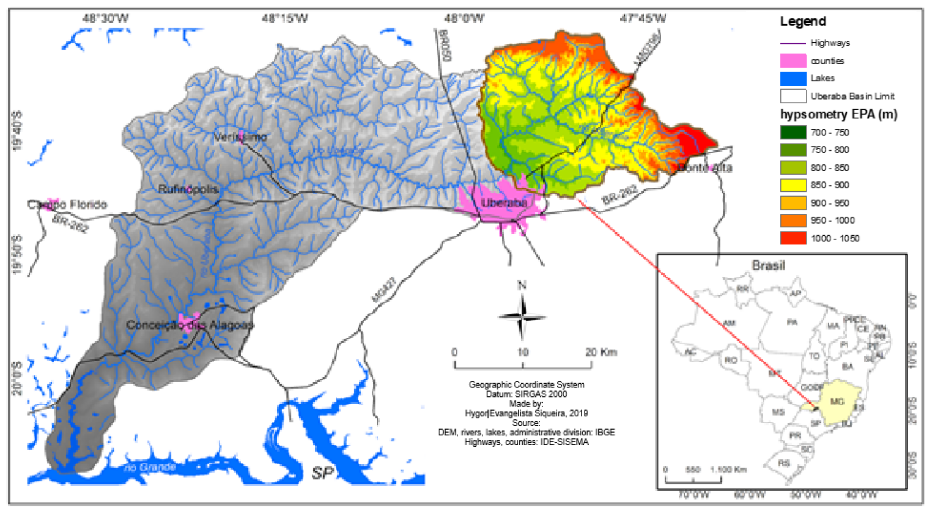
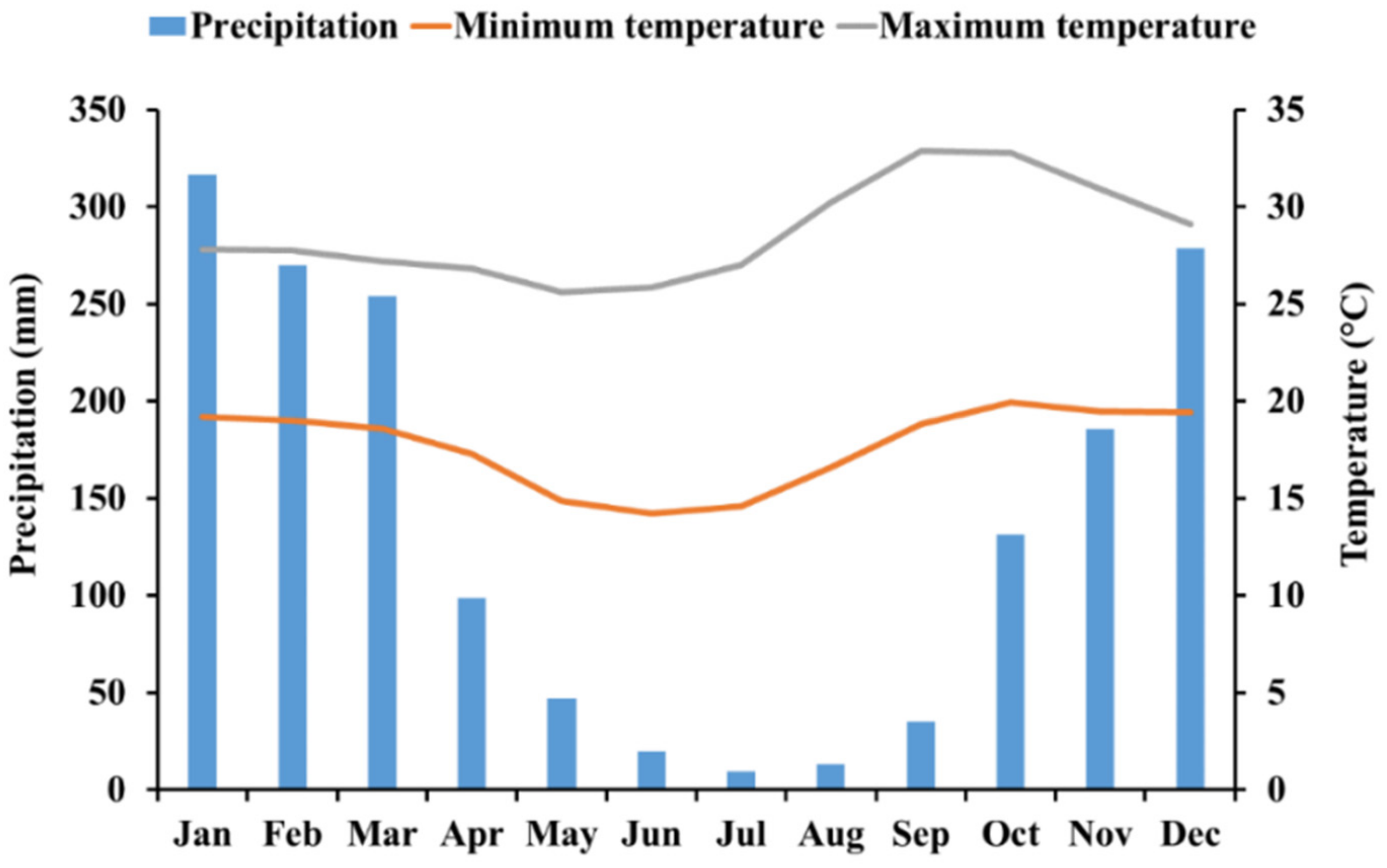
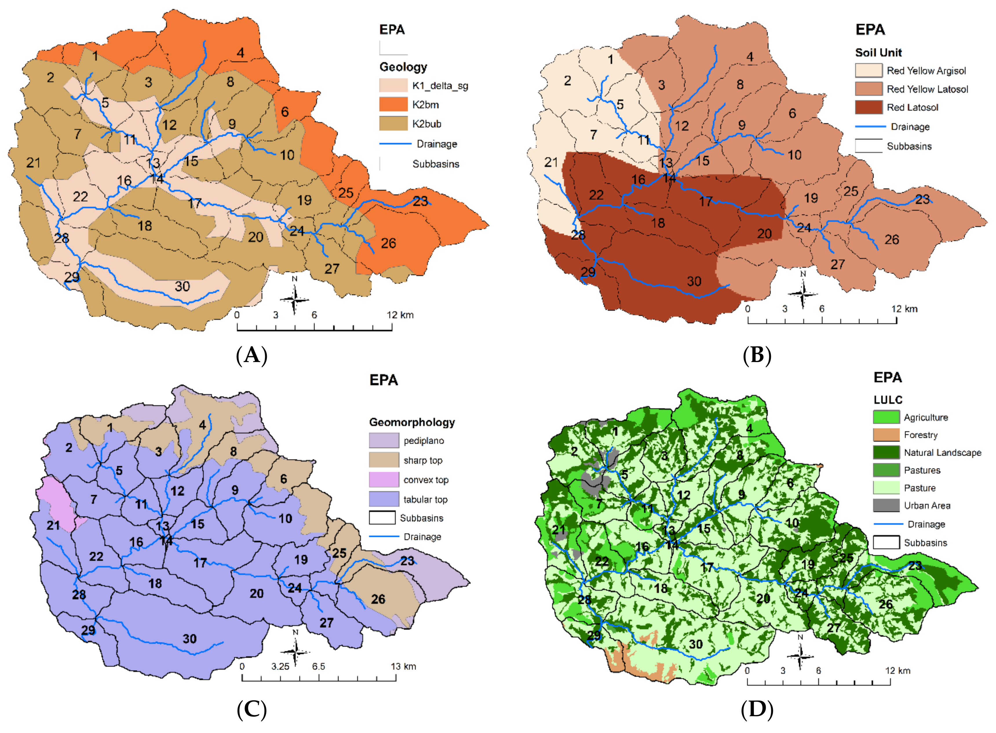
2.1. Study Area

The experimental area is the EPA of the Uberaba River located in Minas Gerais state, Brazil, between longitudes 47°45′ W and 48°00′ W and latitudes 19°35′ S to 19°45′ S (Figure 1). Altitudes varying from 700 m to 1050 m, the basin area covers 525 km2, around 30% of the Uberaba River basin. The Uberaba River flows into Grande River and this into Paraná River.
The EPAs are protected areas defined by the Brazilian Government, regulated by Law 9985, 18 July 2000 [33], that establishes the National System of wildlife protected areas management (SNUC, in Portuguese) aimed to conserve Units of Conservation (UC) to protect the biodiversity and genetic resources within the national territory and waters under the Brazilian jurisdiction. The creation of EPAs has been encouraged as the most effective way to conserve forest remnants [34,35], and especially water recharge areas. Therefore, it is linked to the use of natural resources and, at the same time, to improve the connection of human beings with nature [36].
The area was established as an EPA due to its environmental importance in the region. The area represents the upper portion of the Uberaba River basin that supplies water to Uberaba City, Uberaba Municipality, Minas Gerais state, Brazil. The upper spring supply is a provision of water direct from drainage net to a number of consumers, and is also a source of groundwater to large supplies that are managed by water companies and serve entire communities. According to the Brazilian Institute of Geography and Statistics [37,38] the estimated population of Uberaba City in 2019 was 333,783 people. The area is subdivided into 17 sub-basins and has a drainage net with approximately 454 first-order watercourses, and according to the ‘Mineiro’ Water Management Institute [39], the water is classified as class 2, favoring the use of these waters for public supply, in addition to other uses.
The climate of the region is classified as a semi-dry tropical type, with dry season during April to September and a rainy season from October to March, representing six months of drought [40]. Its average annual precipitation was 1659.3 mm in the period from 1979 to 2013, according to data from ‘Instituto Nacional de Meteorologia do Ministério da Agricultura, Pecuária e Abastecimento’ [41]. The greatest precipitation usually occurs from December to March with values ranging between 253.8 mm and 316.4 mm in March and January, respectively [42,43]. The average minimum and maximum monthly temperature for the same period (from 1979 to 2013) were 17.7 °C and 28.7 °C, respectively (Figure 2).
The geology (A), soil (B), geomorphology (C), and land use (D) of the EPA at the Uberaba River basin are presented on Figure 3.
The geology is mainly in the northeast portion of the Paraná Sedimentary basin, under the geological features of the Central Plateau, formed by the Uberaba formation (k2bub), Marília formation (k2bm), and Serra Geral formation (k1 delta sg) (Figure 3A), [44,45,46]. The soil is formed by organic and inorganic compounds, formed by horizons and change according to climatic influences in a pedological differentiation concerning the source material and the pedogenetic processes [46,47,48,49,50]. The soils were identified in three types, as can be seen in Figure 3B: Red Latosol (Oxisols), Red Yellow Latosol, and Red Yellow Argisol [48]. The geomorphology of the EPA of the Uberaba River basin is characterized by four compartments, which are identified by the tops of the Pediplano, the headwaters, smooth–wavy surface with the convex top, and wavy surface with the sharp top [44,45,46,47,48,49,50] (Figure 3C), occupying 11.13%, 6.56%, 66.68%, and 15.63% of the area, respectively. The main land use of land cover are: agriculture, forestry (eucalyptus), natural landscape (native forest), mining, and urban areas (Figure 3D). Pasture for livestock is predominant, [51,52], and since the 1990s this activity has lost areas to agriculture, which has been gradually advancing in the region. The term agriculture was used for land cover type, “crops”, and meant for cultivation or growing of certain vegetable species to produce food and energy, such as food crops (maize, rice), cash crops (sugarcane, cotton, oilseeds), plantation crops (coffee and rubber) and horticulture crops (fruits and vegetables).

2.2. SWAT Model Data

The ArcSWAT model is an ArcGIS interface tool for soil and water assessment that is a physically-based continues-event hydrologic model developed by the USDA Agricultural Research Service (ARS) [53]. The setup working directory and geodatabases were created to store the parameters needed for SWAT model run. The EPA watershed and sub basins delineation was performed using the Digital Elevation Model (DEM) by Embrapa Relevo Project [54], interpolated to 20 m of spatial resolution converted to SIRGAS 2000, and the slope of the terrain were reclassified into four classes as flat (0–3%), smooth–wavy (3–8%), undulating (8–20%), and mountainous (20–45%) according to [48,49].
The stream definition function was made in the entire area by a watershed delineator method based in a discretization of the Basin areas into smaller increments, such as sub-basins [55,56,57]. The number of sub-basins created was 30, and each one possesses a geographic position in the watershed and is spatially related to one another. The drainage network, the stream juncture points, and the contours (divisors) of each sub-basin were displayed on the map of the Basin (Figure 3). The model incorporates regression equations to describe the relationship between the input and output variables [26].
The following soil classes are found in the basin Red Latosol, Red Yellow Latosol, and Red Yellow Argisol (Figure 3B). The vector files of the soil classes were prepared by Embrapa on a scale of 1:250,000 and acquired from the IBGE database. The data of the tropical soil parameters were inserted into the SWAT database for each soil type.
The runoff volume, as SCS curve number procedure to runoff equation was an empirical model involving rainfall–runoff relationships from small rural watersheds across the U.S. [58]. The model provided a consistent basis for estimating the amounts of runoff under varying land use and soil types [48,49,58]. The retention parameter varies spatially, due to changes in soils, land use, management, and slope; and temporally, due to changes in soil water content.
Daily and monthly climatic data on precipitation, air temperature, relative humidity, wind speed, and solar radiation were obtained from the World Climate Data (USGS). The data were sampled by two automatic meteorological stations of the National Institute of Meteorology—INMET, located in the mesoregion of the Triângulo Mineiro—MG state, Brazil: Conceição das Alagoas meteorological station (A520), at an altitude of 573 m, and the Uberaba weather station (A568), at an altitude of 778 m. To calculate the evapotranspiration, the Penman–Monteith equation was used with monthly climatic data between 1979 and 2013.
The climatic data were precipitation (mm), minimum and maximum air temperature (°C), relative humidity (%), wind speed (ms−1), and solar radiation (MJ/m2 day). To analyze the climate data on the coefficient of variation, the Coefficient of Variation Classification methodology [59], described by Technical Norm No. 171 of November 1989, of the Institute for Forest Research and Studies (IPEF), was used. The climate in EPA of Uberaba River provides indications of the humidity and energy data that control water balance and determine the relative importance of the components of hydrological cycles [26]. To calculate the runoff, the SWAT uses a modified Soil Conservation Service Curve Number (SCS CN) methodology. The SCS CN is a function of the soil permeability, land use, and antecedent soil water conditions and is calculated by the cover, hydrologic soil group, land use, treatment or practice, and hydrologic condition A, B, C, and D [38].
The land use map was made by The Brazilian Annual Land Use and Land Cover Mapping Project (MapBiomas), from Brazilian 1985-2020 database, located at https://mapbiomas.org/en/project, accessed on 14 February 2020. Land use data were determined considering the coverage of the predominant rural area and the coverage of the urban area, considering the land uses described on [60,61], described in Table 1, and Figure 3D.
To model purposes [60,61,62,63,64,65,66], the SWAT model divided the watershed into a sub-basin and, in turn, into the hydrologic response units (HRUs) [26]. Each HRU was a homogeneous unit that comprised the unique land cover, soil, and slope attributes.
The SWAT quantified the relative impacts of vegetation, soil, management, and climate change within each HRU. The output of the hydrological model (e.g., runoff, sediments, and nutrients) was calculated in each HRU and then summed to another HRU of the same sub-basin to compute the total loading from the sub-basin. The SWAT model was executed on a monthly basis with a warm-up period of 3 years (from 1979 to 1981) with the aim of (i) helping to minimize the model values for the initial hydrological conditions, and (ii) ensuring the establishment of basic flow conditions and hydrologic process equilibriums [24].
All LULC parameters were obtained from the SWAT database, excepted the BLAI (maximum leaf area index), GSi (canopy stomatal conductance), and OV_N (Manning coefficient for the soil surface) of the vegetation covers. These parameters were changed to better represent the tropical conditions (Table 2).
The hydrological cycle is based on water balance equations [62,66] and the results provide, in addition to the physical description of the compartments, the total runoff value of the EPA of the Uberaba River sub-basins. When the rains fall, the drops are intercepted according to the morphometric characteristics of the vegetation cover. The redistribution component of the SWAT model uses a rainwater tracking technique to predict the flow of water entering the system on the hydrological cycle processes.

2.3. Model Calibration and Uncertainty Analysis

2.3.1. Calibration and Validation of Streamflow Data

For the calibration and validation of the SWAT model, we used streamflow data of the website of the National Water Agency [67], from the Uberaba fluviometric station, identified by code 61794000 corresponding to the point flow, under the coordinates 19°43′48″ S and 47°58′48″ W. This hydrometric station was located approximately 4.8 km from the mouth of the Uberaba River and was used for the calibration and validation of the SWAT model from 1982 to 1987 and 2006 to 2010, respectively. The discharge was calibrated at a monthly time step rather than a daily time step because, despite the precipitation being available at the daily scale, the observed streamflow had daily data with gaps but is complete and reliable at the monthly scale. Despite monthly water balance models not performing as well as daily water balance models in simulating monthly runoff, the research developed by [68,69] showed that monthly calibration is particularly valuable for applications where one is primarily interested in monthly, seasonal, and annual streamflow volumes, and is a viable alternative to daily calibration when no daily streamflow data are available. Finally, the monthly calibration has the advantage of making the calculation process faster, so it is possible to quickly carry out a large number of simulations for parameter sensitivity and uncertainty analyses [69,70].

2.3.2. Parameter Selection

Model calibration was focused on optimizing seven parameters, which were identified using the sensitivity analysis tool. This method combines Latin-Hypercube and one-factor-at-a-time sampling. The parameters are ranked according to their sensitivities and the first three parameters (GWQMN, EPCO, and GW_DELAY) had a significant influence on calibration (p ≤ 0.05) (Table 3).
To calibrate the hydrological model, it was necessary to change the parameters that govern (i) the surface water processes, including the curve number (CN), (ii) both evapotranspiration and soil moisture including the parameters of the soil evaporation compensation factor (ESCO) and plant uptake compensation factor (EPCO), and (iii) the parameters that control the subsurface water processes, including the flow threshold depth of water in a shallow aquifer (GWQMN), groundwater delay (GW_DELAY), and deep aquifer percolation fraction (RCHRG_DP), and Baseflow alpha factor (ALPHA_BF) [55,56,57,58,59,60,61,62,63,64,65,66,67,68,69,70,71,72].
The CN2 parameter was raised during calibration, which has the effect of increasing the amount of surface runoff generated from rainfall. The ESCO parameter remained close to the maximum value (0.943) meaning that the predicted streamflow values became closer to the observed streamflow when the ESCO value was at its maximum. This parameter controlled the soil evaporative demand that was to be met from different depths of the soil [70]. Thus, raising the ESCO value decreased the soil depth to which SWAT can satisfy potential soil evaporative demand [69,70,71], thus decreasing soil evaporation and ET and increasing total water yield, streamflow, and baseflow [71,72]. In turn, the EPCO parameter was lowered (0.022) because the water uptake demand for plants was met by higher layers in the soil. This way, less water was transferred from the lower layers in the soil to atmosphere through evapotranspiration [24,25,26,27,28].
The shallow aquifer contributed baseflow to the main channel or reached within the sub-basin. Baseflow was allowed to enter the reach only if the amount of water stored in the shallow aquifer exceeded a threshold value specified by the user which was defined by GWQMN parameter [73]. For a low value of GWQMN, SWAT produced more base flow. The effect of this parameter on baseflow influenced the streamflow as well [72]. The low value of GWQMN (357 mm) corresponded to high streamflow, which was in accordance with observed streamflow values. The ALPHA BF described the rate at which groundwater entered a stream. The approximate value of 0.3 was estimated in this study. Compared with commonly used values, which range from 0.3 to 1 [74], the baseflow recession constant of 0.3 was small, suggesting slow drainage and major storage in shallow aquifers. To adjust the baseflow, it was also necessary to raise the value of GW_DELAY, i.e., increase the time delay between water exiting the soil profile and entering the shallow aquifer (about 260 days). Indeed, this value can be considered reasonable because the soils present in the catchment are deep and have Red-Yellow Argisol (PVA) which is characterized by low hydraulic conductivity. Finally, for an optimal model, adjustment was necessary to increase the deep percolation (RCHRG_DP = 0.247). The RCHRG_DP is a fraction of the total daily re-charge that can be routed to the deep aquifer. The amount of water moving from the shallow aquifer due to percolation into the deep aquifer was correlated to the aquifer percolation coefficient, i.e., the amount of recharge entering both aquifers [62,73].

2.3.3. The SUFI-2 Procedure and the Statistical Evaluation Criteria

The Sequential Uncertainty Fitting (SUFI-2) routine, which is linked to SWAT under the platform of SWAT Calibration and Uncertainty Programs (SWAT-CUP) 2012 [75], was used to model the calibration and estimation of both parameter and predictive uncertainty at the EPA of the Uberaba River basin. SWAT-CUP 2012 is a standalone computer program developed for calibration and validation of SWAT model [75] and SUFI-2 is acknowledged as a powerful tool for making calibration and uncertainty analysis of the SWAT model [75,76,77]. In SUFI-2, parameter uncertainty is reported using a multivariate uniform distribution in a parameter hypercube, while the model output uncertainty is derived from the cumulative distribution of the output variables [77,78].
The objective function selected as the calibrated parameter set was the Nash–Sutcliffe Efficiency (NSE). It was also used as the coefficient of determination (R2) and the percent bias (PBIAS) and standardized RMSE (RSR) to assess the model performance. The NSE is commonly used for reflecting the overall fit of a hydrograph because it is very sensitive to high extreme values (due to the squared differences) [24,66]. NSE values vary from −∞ to 1, with a value of 1 indicating that the simulated and observed discharge data are perfectly matched. This way, NSE values greater than 0.5 means that the model is appropriate and good for the simulation of maximum streamflow [79]. The goodness-of-fit indicator, R2, describes the proportion of the variance in measured data explained by the model. R2 ranges from 0 to 1, with higher values indicating less error variance. This indicator has been widely used for model evaluation, and values granter than 0.5 and 0.75 have been considered satisfactory and very good performance of the model, respectively [78].
The PBIAS values indicate the deviations between the mean simulated and observed streamflow, expressed as a percentage. The optimal value of PBIAS is 0.0, with low-magnitude values indicating accurate model simulation. A positive value of PBIAS indicates an underestimation bias while a negative value indicates an overestimation one [75,79]. The RSR is the ratio of the root mean square error (RMSE) to the standard deviation of measured data (STDEVobs). The RSR varies from 0 to a large positive value. The optimal value is 0 which indicates zero RMSE or residual variation and therefore perfect model simulation [79]). In general, these goodness-of-fit indicators are considered satisfactory whenever R2 and NS are greater than 0.5, RSR less than 0.7 and PBIAS ranges between less than ±25% for the streamflow [79,80].

2.4. Afforestation and Pasture Scenarios

The land use scenarios were selected in order to verify the phenomena of replacement of land occupation in natural landscapes. Anthropogenic actions contribute to the degradation of natural resources, including water resources. Originally created by Law 6902/1981, environmental protection areas are now regulated by Law 9.985/00, the National System of Nature Conservation Units (SNUC). The EPA can be established in areas of public or private domain, by the Union, States, or municipalities, without the need for expropriation of private lands. The status of the EPA is an area for protection and conservation of the sustainable land use category as the law allows for human occupation and sustainable production. Therefore, there was not yet an orderly human occupation of the area and the sustainable use of its natural resources.
The activities and uses developed in these areas are subject to specific rules and the owner must establish the conditions for research and public visitation, subject to legal requirements and restrictions. To evaluate the hydrological response to land use changes at the EPA of the Uberaba River basin, two scenarios were considered. Forest Scenario supposes that all current PAST and AGRL will be changed to FRST representing a 97% increase in FRST area over the entire catchment.
The scenarios of the land uses changed from 32.6% to 97.1%—forest or 53.3% to 97.1%—pastures, and the areas were investigated to better understand the environmental conditions or watershed potential as the land use modifies to pasture or crops scenarios.
Pasture Scenario supposes that all current FRSE and AGRL will be converted to PAST, representing a 97% increase in PAST area over the entire catchment. Meanwhile, the rest of the land covers, Residential-Medium Density (URMD), Industrial (UIDU), and Eucalyptus (EUCA), will remain unchanged.
The scenarios were chosen due to the link between process studies of hydric balance change and impact assessments to analyze the indication of what the future might achievably be like. At the EPA, the land uses are changed in environmental systems of watershed from natural landscape transformed in pasture lands emphasizing the functional role of land for economic activities.
The study will show basic assumptions to ensuring sustainable conditions and might also trigger feedback to the system and vulnerability conditions, such as the forest management nexus in the EPA versus pasture consequences on water resources. These two land use change scenarios (i.e., afforestation and pasture) were based on present land use conditions and potential future land use. The percentage areas of the current land use and the change scenarios are shown in Figure 4.

3. Results

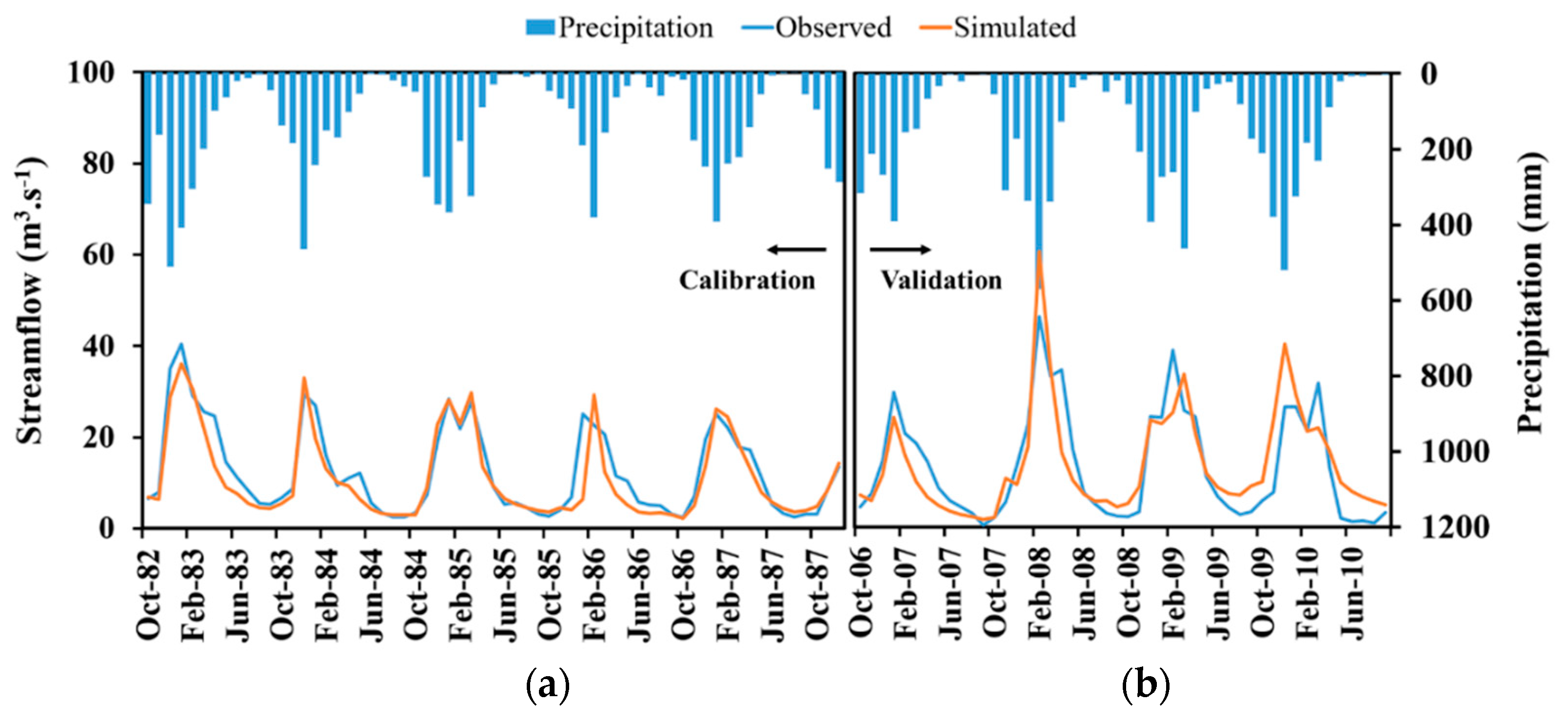
3.1. Calibration and Validation of the Streamflow

The streamflow was calibrated to a 5-year period (1982–1987) and validated to a 4-year period (2006–2010), both monthly. Figure 5 shows the agreement between the observed and the simulated streamflow for both calibration and validation periods. The visual analysis of the simulated hydrograph reproduced the measured discharge reasonably well and closely replicated the temporal variation, as well as the mean monthly precipitation. Table 4 depicts the goodness-of-fit indicators for the streamflow calibration and validation based on the NSE, R2, PBIAS, and RSR. The goodness-of-fit indicators for the streamflow show good and very good performance of the model in both calibration and validation. The analysis of the NSE values is 0.82 (very good) and 0.70 (good) for both calibration and validation respectively. The R2 shows good and very good performance of the model with values of 0.85 and 0.72 for calibration and validation, respectively [78]. The PBIAS values indicate some deviations between the mean simulated and observed streamflow. In calibration, it shows an underestimation of 12% of simulated streamflow, and in validation a slight overestimation in 4% of cases. These values mean that the performance of the SWAT model in estimating the mean streamflow is satisfactory and very good in both calibration and validation, respectively (Figure 5) [79]. The analysis of the RSR shows values of 0.42 (very good) and 0.55 (good) for calibration and validation, respectively [79].

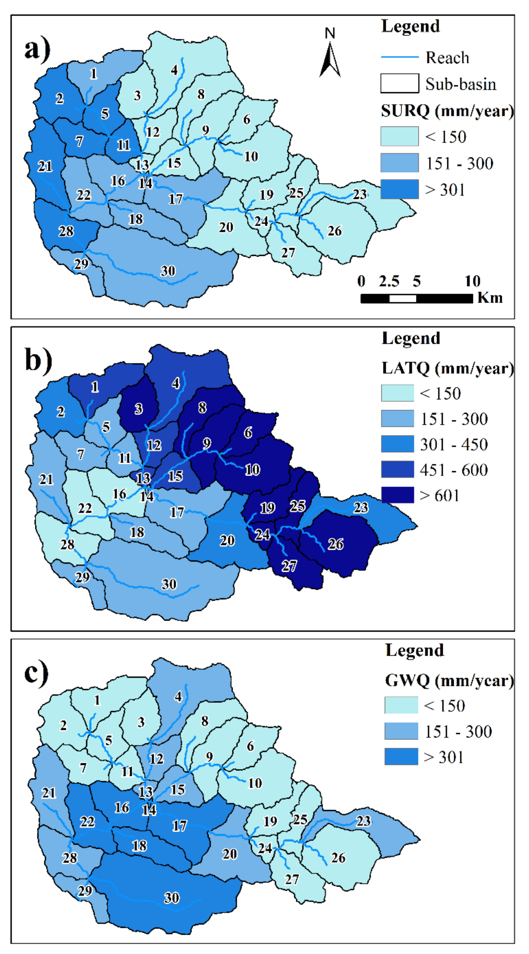
3.2. Water Balance of the Current Land Use

The water balance of the Uberaba River basin is presented in Table 5. The streamflow and actual evapotranspiration (ET) represented 44% and 51% of the precipitation respectively and the remaining 5% percolate to the deep aquifer. The largest amount of water that reaches the river comes from the lateral flow (48%), and the remaining flow is from the surface and groundwater with 25% and 27%, respectively (Table 5). Figure 6 shows the spatial distribution (in each sub-basin) of surface runoff (SURQ), lateral runoff (LATQ), and groundwater (GWQ) in the current land use. The values of flow components are expressed in mm and are an average annual between 1982 and 2013 in the Uberaba River basin. The spatial distribution of flow components in the catchment is very uneven, i.e., the average annual of surface flow was greater in the western sub-basins (>300 mm/year), while the lateral flow is major in the eastern and northern sub-basins (>450 mm/year) and the groundwater flow is higher in the southern sub-basins (>300 mm/year).

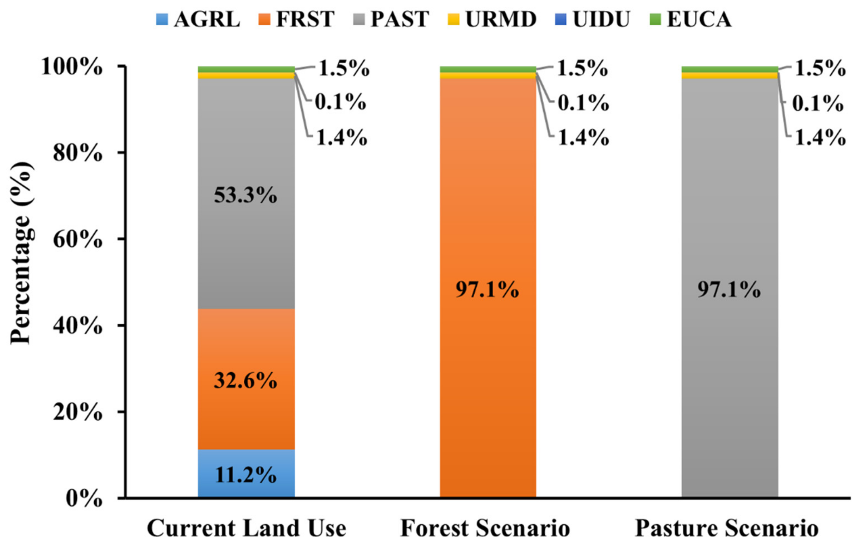
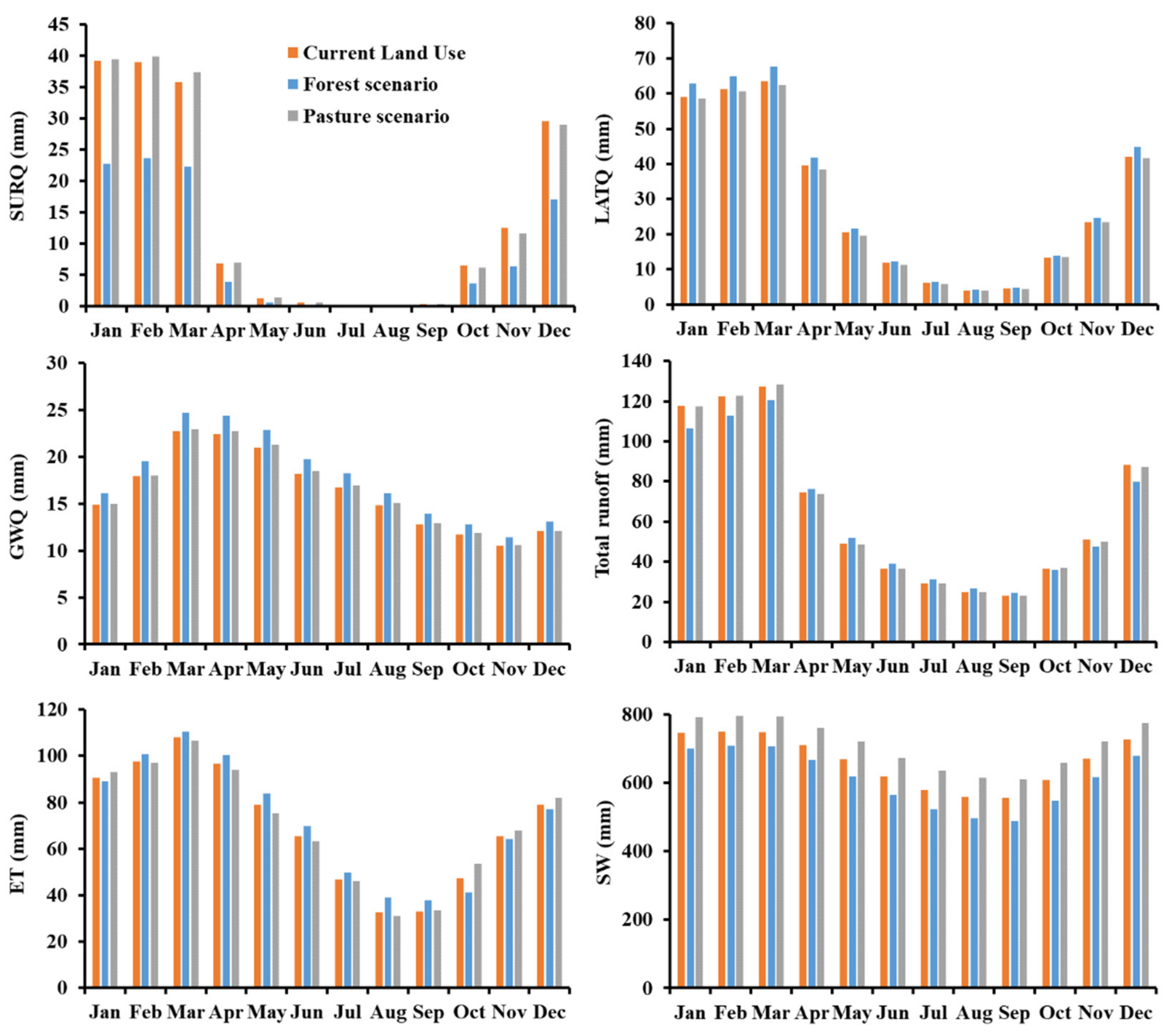
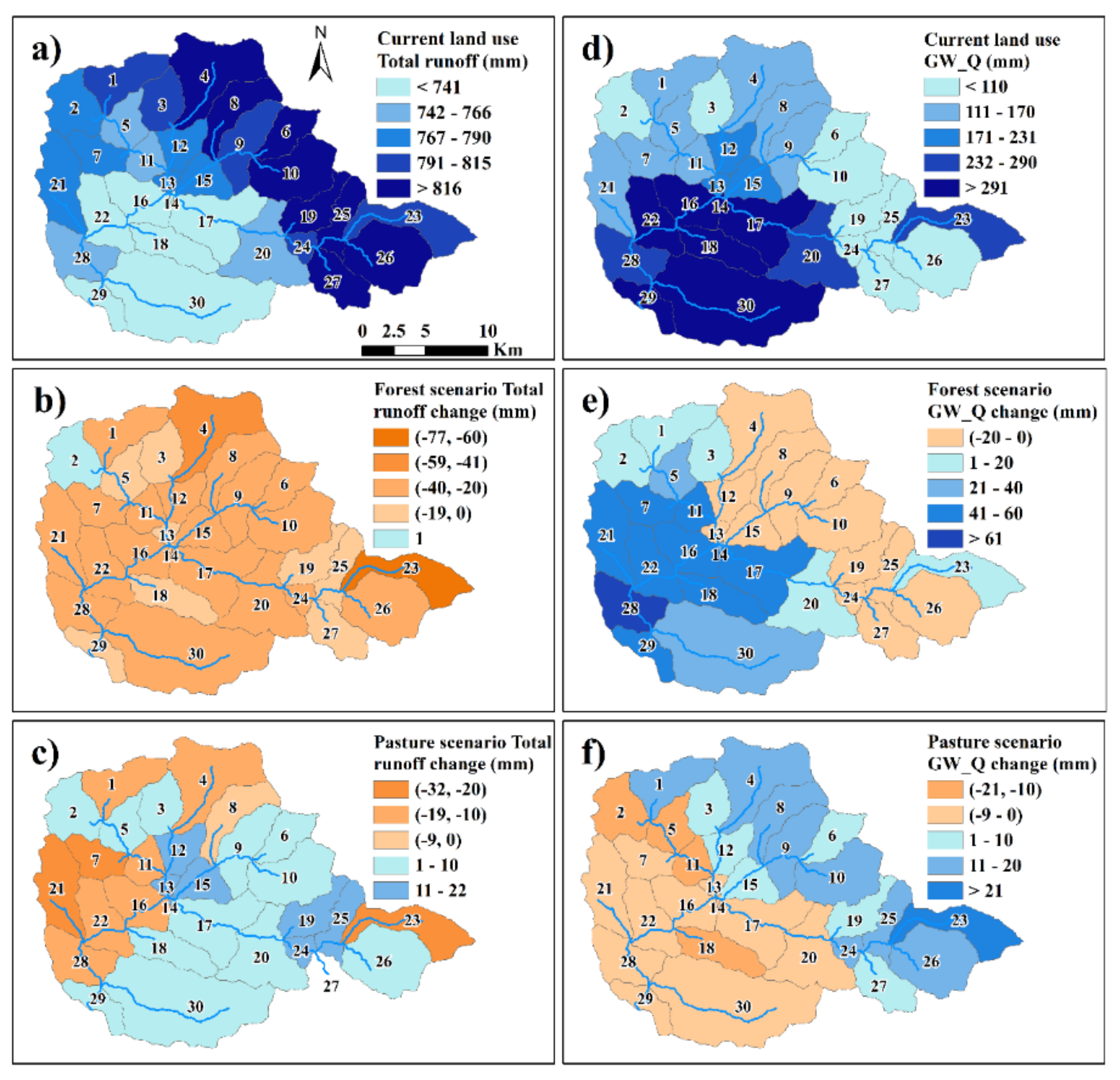
3.3. The Current Land Use, and Forest and Pasture Scenarios

The calibrated SWAT model was applied to simulate the monthly SURQ, LATQ, GWQ, total runoff, ET, and soil water (SW) under the current land use, and the scenarios of forest and pasture (Figure 7). The results show that all components of water balance presented monthly variations, with values generally greater between December and May, which corresponds to the wet season (Summer and Autumn), and minor values between June and November, which corresponds to the dry season (Winter and Spring) (Figure 7). The monthly SURQ of the forest scenario was the component that showed high differences under land-use scenarios, with the most changes occurring during the wet season from December to May. Less remarkable changes were observed in other components of water balance in the forest scenario, and all components in the pasture scenario (Figure 7). Table 6 summarizes the average annual values of current land use, and the average annual values change and percentage change of both scenarios for the same components analyzed in Figure 7. The 64.5% increase in FRSE area led to a decrease of 71.1 mm (45.3%) in the surface runoff, 11 mm (4.8%) in total runoff, and 48.5 mm (7.1%) in soil water; and an increase of 21 mm (5.7%) in lateral flow, 17.1 mm (2.6%) in groundwater, and 23.2 mm (2.9%) in evapotranspiration (Table 6). The 43.8% increase in PAST area led to an increase of 1 mm (3%) in surface flow, 2.1 mm (2%) in groundwater, 2.5 mm (0.2%) in evapotranspiration, and 48.3 mm (6.8%) in soil water; and a decrease of 5.4 mm (1.5%) in lateral flow and 0.8 mm (0.6%) in total runoff.
Figure 8 shows the spatial distribution (in each sub-basin) and annual average of total runoff and GWQ in current land use, and the changes under forest and pasture scenarios. The spatial distribution of total runoff and GWQ in current land use is distinct. While the total runoff is greater in the northern sub-basins (>790 mm), the GWQ is higher in the southern sub-basins (>230 mm) (Figure 8a,d). In the forest scenario, the decreased total runoff observed in Figure 8b and Table 6 is found evenly distributed across the basin, being that most sub-basins show between −20 and −40 mm. The increase of GWQ observed in Figure 8e and Table 6 is found in the western and southern sub-basins (until 60 mm). Contrarily, in the northern sub-basins we detected a decrease until −20 mm of GWQ. In the pasture scenario, the decreased total runoff observed in Figure 8c and Table 6 only occurred in the western and some northern sub-basins (until −32 mm); in the remaining sub-basis we observed an increase (until 22 mm). Contrary to total runoff, the GWQs observed in Figure 8 and Table 6 increase, but the spatial distribution shows that the increase only occurs in the northern sub-basins (until 21 mm), while in the southern sub-basins we observed a decrease (until −21 mm).

4. Discussion

4.1. Limitations of the Simulation

Although calibration results are considered good, there are some factors that com-promise the model performance. In this work, the two factors that seem to most influence the flow estimation are the rain gauge density and the accuracy of the hydrometric gauges. The performance of hydrological modeling depends largely on the quality of the rainfall data and the density of rain gauges. The authors of [80,81] analyzed the effect of the high variability in rainfall on the uncertainty of the calibrated model, and they suggest that the high variability in rainfall can be attributed to the low rain gauge density. In fact, the density of the rainfall input data contributes significantly to the level of uncertainty in the simulated streamflow because as the variability in rainfall increases, the uncertainty of calibrated model also increases. Thus, reducing the variability in rainfall input data and accurately estimating the rainfall data used for calibrating the model could lead to a significant improvement in simulated streamflow thereby reducing the level of uncertainty of the model. In addition, this low density difficultly represents the orographic effect on the precipitation, i.e., some climate stations are within lower altitude values and consequently cannot represent the orographic effect on the precipitation rates. In the study area, the rain gauges are located at an altitude of 573 and 778 m, i.e., in valleys, within the orographic “shadow” of the surrounding mountains that reach 1043 m of altitude.

4.2. Water Balance Analysis

The spatial distribution of the surface flow, lateral flow, and groundwater flow in current land use are not equal in the entire basin and their variability has different sources. The spatial distribution of the surface flow is similar to the soil type map (Figure 3c), while the lateral flow represents the different slopes that occur in the basin, and the groundwater represents both the soil type and slope. Indeed, the higher surface flow in the western sub-basins of the catchment occurs under Red-Yellow Argisol (PVA). This soil has poor aeration during the rainy season due to low hydraulic conductivity at the top of the Bt horizon, resulting in high surface runoff and high erodibility [82]. Meanwhile, in the southern and northern/eastern sub-basins there is Red Latosol (LV) and Red-Yellow Latosol (LVA), respectively. These soils are characterized by good internal drainage that is attributed to their great porosity. As a whole, they have low erodibility associated with low flow potential superficial [82].
The spatial distribution of lateral flow is a faithful representation of the slope, being that it is greater in the eastern and northern sub-basins of the catchment where it is a predominantly steep slope. Indeed, the slope has an important role in streamflow and sediment yield. Several authors, in their works, also obtained the similar results [83,84]. Ref. [83] using the SWAT in the Upper Danube Basin (which covers about 132,000 km2 across Austria, Germany, Czech Republic, and Slovakia) showed that default hillslope length (the SWAT method) resulted in large overestimations of lateral flow. In addition, [84] reported that the SWAT for the calculation of lateral flow velocity, in HRUs, overestimates the amount of lateral flow in steep slopes. The same authors argue that the SWAT also drives an increasing underestimation of surface runoff in increasing slope gradients.
The spatial distribution of groundwater flow reflects the soil type in the southern and western sub-basins and the slope in the eastern and northern sub-basins of the catchment. In the southern sub-basins, the major groundwater flow is associated with Red Latosol due to its good internal drainage. In the eastern and northern sub-basins, the lower groundwater flow is associated with a steep slope. Indeed, the higher lateral flow drives a decrease in the amount of soil water that is available for percolation to the groundwater. This observation can explain the lower groundwater flow in steep slope sub-basins. The same results were obtained by the authors [83,84].
In the EPA of the Uberaba River basin, the streamflow and ET represented 44% and 51% of the precipitation, respectively (Table 5). These values are different from work developed by [66] in Atlantic Forest of the Pomba River basin, located in Minas Gerais state and Rio de Janeiro states. They performed tests on water balance in SWAT and the values of ET were 69% and 63% for calibration and validation respectively, and 27% and 30% for calibration and validation of the streamflow, respectively. In addition, the percentage of water that reaches the river by surface, lateral, and groundwater flows were different. They presented a similar percentage of lateral and groundwater flows, between 46% and 48% for calibration and validation. They obtained 6% of the streamflow from the surface flow for calibration and validation against 25% in the EPA of the Uberaba River basin and the opposite for groundwater flow, with approximately 48% in the Pomba River Basin against 27% in the EPA. Only the lateral flow presented an equal percentage near 48% in both basins. The differences between both basins can be due to major area of forest and eucalyptus in the Pomba River basin that leads to an increase of infiltration and consequently less surface flow and major ET. In addition, the Red-Yellow Latosol with good internal drainage as dominant type soil in Pomba River basin contributed to less surface flow.
The uncertainties represent limitations for decision making with respect to the mitigation of impacts, based on a paradigm of optimization. Nevertheless, the rural farmers need the integration of knowledge that they consider the multiple stressors that condition the environment of decision of the EPA. Application of exploratory analysis, which consider multiples scenarios, systematically explores the implications of a wide range of hydrological conditions and policies [5,6,7,8,9,10,11].

4.3. Components of the Water Balance of the Current Land Use Forest and Pasture Scenarios

The Uberaba River basin is inserted in a summer rainfall-dominant region, that occurs between December and May, and a predominantly dry winter that occurs between June and November (Figure 8). This inter-annual distribution of rainfall is well represented by the monthly variations in SURQ, LATQ, GWQ, total runoff, ET, and SW simulated by SWAT in the current land use. In addition, the changes under forest and pasture scenarios differed across months. The greater changes occurred during the wet season (December–May) and the SURQ, LATQ, GWQ, and total runoff were the components that best represented these changes. In the forest scenario, a decrease of the surface flow, total runoff, and soil water, and an increase of the lateral flow, groundwater flow, and evapotranspiration were observed. Between all components, the surface flow presented the major percentage change (average of −45%) at annual time scales (Table 6).
The increases of infiltration were due to increases in soil organic matter improved by the forest. Indeed, the increase in the lateral flow and groundwater flow, in the study area, indicates that the Atlantic Forest contributes to an increase of water infiltration into the soil. The results showed that the increase of infiltration does not necessarily drive the increases in total runoff and soil water: on the contrary, they decreased. This occurs because trees with their deep root systems can extract more water from shallow aquifer storage, and, can transpire more due to larger leaf area [85,86,87]. However, the effect of the vegetation cover on soil moisture content is still questionable. This is because if it is true that the increase of vegetation cover increases the transpiration loss and the rainfall interception, it also triggers the decreases of evaporation loss through shading. This way, the shading of canopy vegetation reduces the direct radiation absorption, leading to lower soil temperature and soil evaporation rates, followed by greater soil moisture [88]. The same authors argue that the effect of vegetation cover on the soil water content may be due to climate and the length of dry or wet periods.
The EPA of the Uberaba River Basin protected area was created by the local municipal government with the main goal of bringing environmental benefits to Uberaba’s society. Concerning preservation policy, the local actors established a unit of conservation within an economic interest as agricultural and livestock production systems, following the Brazilian Forest Code to land use regulation in rural estate properties and the improvement of policies on economic and ecological zoning (ZEE) [29].
The water environmental interests should have strong incentives to seek better management at the EPA of the Uberaba River Basin. This study also shows a way of looking at the effect of land use change in watersheds on the volume of water available, as a subsidy to payments for ecosystem services (PES) system, that can come about with the establishment of catchments on springs, and the hydrological benefits that will come from productive pasture potential of land to be changed into forest land with more biodiversity and hydrological functioning. Those incentives should encourage groups of rural producers to adopt policy platforms and lobbying strategies that can improve the environmental soil and water sustainability. The environmental interests of land use, land changes, and the preservation of natural lands may benefit from at least some of the owners of rural properties over conservation units for preserving the natural ecosystem in a biological function. The social and economic functions of the land are stronger when the land is used. The government should create a protected area seeking the needs of major local production systems as main industries and subnational efforts to reconcile competing interest yields on average weaker environmental policy at a local level of government. The creation of payment for environmental service policies need to consider the water production in each area along rivers and springs along with the areas that must be preserved by the Brazilian Forest Code. The PES schemes are relatively new and policies are needed to support positive environmental externalities through the transfer of financial resources from beneficiaries of certain environmental services to those who provide these services or are fiduciaries of environmental resources. The area of the EPA of the Uberaba River Basin is a perfect area to start those policies to benefit local rural producers and water uses in the Uberaba municipality which, according to data from the Brazilian Institute of Geography and Statistics (IBGE), has approximately 337,000 inhabitants.

5. Conclusions

The hydrological discharge of headwater sub-basins showed space–time variation in magnitude on the 30 sub-basins at EPA of the Uberaba River basin. The SWAT-T model was used to analyze the hydrological sensitivity of a tropical catchment in Minas Gerais state, Brazil. To better represent the vegetation types for tropical areas, the parameters BLAI, GSi, and OV_N were changed. After that, we created land use changes on forest and pasture scenarios.
The land use changes on forest and pasture scenarios showed that all components of water balance presented monthly variations. The greater changes occurred during the wet season (December–May) in the monthly SURQ of the forest scenario. The results showed that a 64.5% increase of FRSE area led to a decrease of 71.1 mm in surface runoff, 11 mm in total runoff, and 48.5 mm in soil water; and an increase of 21 mm in lateral flow, 17.1 mm in groundwater, and 23.2 mm in evapotranspiration. The 43.8% increase in PAST area led to an increase of 1 mm in surface flow, 2.1 mm in groundwater, 2.5 mm in evapotranspiration, and 48.3 mm in soil water; and a decrease of 5.4 mm in lateral flow and 0.8 mm in total runoff.
The hydrological model indicated the main areas of spatial optimal water flow. Considering economic values, those areas should encourage the government’s policy of incentive platforms that can improve environmental soil and water sustainability. The creation of payment for environmental service (PES) policies should consider the water production and the areas further along with the areas that must be preserved by the Brazilian Forest Code and the Conservation Units should be an environmental protection area to hydrological economic interests. Furthermore, the methodology employed in this study can be further applied to other tropical catchments for LULC impact assessments on water resources.
Information processing models suggest that a variety of scenario characteristics may affect watershed ecosystems in hypothetical testing scenarios in ways that can influence the degree to which a landowner engages with and carefully considers information about the land uses of pasture and forest. Examinations of the SWAT Processing Model suggest that details underscoring the importance of and accountability for a land use decision lead to the application of better management practice on rural lands. For example, hypothetical scenarios of pasture and forest might include information linking the hydrological cycle to a sub-basin unit, thereby increasing the sustainability management of forest and forest livestock will be a better choice for management practices. The management of forest and pasture areas and the accountability of a better land use policy are important to consider, as they are more likely to naturally occur in a watershed ecosystem, as opposed to hypothetical scenarios where the influence of forest and pasture are often absent.

Author Contributions

Conceptualization, M.S.d.M.M., T.C.T.P. and C.A.V.; methodology, T.C.T.P. and R.M.B.S.; software, L.F.S.F., T.C.T.P. and R.M.B.S.; validation, T.C.T.P. and R.M.B.S.; formal analysis, F.A.L.P., T.C.T.P. and M.Z.; investigation, M.S.d.M.M., T.C.T.P. and C.A.V.; resources, M.S.d.M.M. and T.C.T.P.; data curation, M.S.d.M.M., T.C.T.P. and R.M.B.S.; writing—original draft preparation, M.S.d.M.M., T.C.T.P., R.M.B.S., M.Z. and T.C.T.P.; writing—review and editing, F.A.L.P., M.S.d.M.M., V.L.A., T.C.T.P. and R.M.B.S.; visualization, F.A.L.P. supervision, T.C.T.P. and L.F.S.F.; project administration, T.C.T.P. and L.F.S.F.; funding acquisition, M.S.d.M.M., T.C.T.P. and L.F.S.F. All authors have read and agreed to the published version of the manuscript.

Funding

The present study was carried out within the framework of the Post Graduation Research Program of ‘Coordenação de Aperfeiçoamento de Pessoal de Nível Superior’ (CAPES); Conselho Nacional de Desenvolvimento Científico e Tecnológico (CNPq); Agência do Ministério da Ciência, Tecnologia, Inovações e Comunicações (MCTIC); and Land Use Policy Brazilian Group (PolUS). For the author integrated in the CITAB Research Centre, the research was further financed by the FEDER/COMPETE/POCI—Operational Competitiveness and Internationalization Program, under Project POCI-01-0145-FEDER-006958, and by the National Funds of FCT—Portuguese Foundation for Science and Technology, under the project UIDB/AGR/04033/2020. For the author integrated in the CQVR, the research was further financed by National Funds of FCT—Portuguese Foundation for Science and Technology, under the project UIDB/QUI/00616/2020.

Institutional Review Board Statement

Not applicable. The study was conducted not involving humans or animals.

Informed Consent Statement

Not applicable.

Data Availability Statement

Not applicable.

Acknowledgments

The authors would like to thank: the Coordination of Improvement of Higher Education Personnel (CAPES) for the scholarship; the National Council for Scientific and Technological Development (CNPq) for Research funds; the Agronomy (Soil Science) Post-Graduation Program from School of Agricultural and Veterinary Sciences, São Paulo State University (UNESP); The Land Use Policy Research Group—PolUS; the Federal Institute of Education, Science and Technology of ‘Triângulo Mineiro’ region (IFTM).

Conflicts of Interest

The authors declare no conflict of interest.

References

  1. Nugroho, P.; Marsono, D.; Sudira, P.; Suryatmojo, H. Impact of Land-use Changes on Water Balance. Procedia Environ. Sci. 2013, 17, 256–262. [Google Scholar] [CrossRef] [Green Version]
  2. Pumo, D.; Arnone, E.; Francipane, A.; Caracciolo, D.; Noto, L.V. Potential implications of climate change and urbanization on watershed hydrology. J. Hydrol. 2017, 554, 80–99. [Google Scholar] [CrossRef]
  3. Teklay, A.; Dile, Y.T.; Asfaw, D.H.; Bayabil, H.K.; Sisay, K. Impacts of land surface model and land use data on WRF model simulations of rainfall and temperature over Lake Tana Basin, Ethiopia. Heliyon 2019, 5, e02469. [Google Scholar] [CrossRef] [PubMed]
  4. Gao, Y.; Chen, L.; Zhang, W.; Li, X.; Xu, Q. Spatiotemporal variations in characteristic discharge in the Yangtze River downstream of the Three Gorges Dam. Sci. Total Environ. 2021, 785, 147343. [Google Scholar] [CrossRef] [PubMed]
  5. Calder, I.; Aylward, B. Floresta e inundações: Mudando para uma abordagem baseada em evidências para a gestão integrada de bacias hidrográficas e inundações. Water Int. 2006, 31, 87–99. [Google Scholar] [CrossRef]
  6. Crétaz, A.L.; de la Barten, P.K. Land Use Effects on Streamflow and Water Quality in the Northeastern United States; CRC Press: Boca Raton, FL, USA; Taylor & Francis Group: Abingdon, UK, 2007; ISBN 9780429694905. [Google Scholar]
  7. Viola, M.R.; Mello, C.R.; Beskow, S.; Norton, L.D. Impacts of Land-use Changes on the Hydrology of the Grande River Basin Headwaters, Southeastern Brazil. Water Resour. Manag. 2014, 28, 4537–4550. [Google Scholar] [CrossRef]
  8. Lepeška, T.; Radecki-Pawlik, A.; Wojkowski, J.; Walega, A. Hydric potential of the river basin: Prądnik, Polish Highlands. Acta Geophys. 2017, 65, 1253–1267. [Google Scholar] [CrossRef]
  9. Oudin, L.; Salavati, B.; Furusho-Percot, C.; Ribstein, P.; Saadi, M. Hydrological impacts of urbanization at the catchment scale. J. Hydrol. 2018, 559, 774–786. [Google Scholar] [CrossRef] [Green Version]
  10. Wojkowski, J.; Młyński, D.; Lepeška, T.; Wałęga, A.; Radecki-Pawlik, A. Link between hydric potential and predictability of maximum flow for selected catchments in Western Carpathians. Sci. Total Environ. 2019, 683, 293–307. [Google Scholar] [CrossRef]
  11. Lepeška, T.; Wojkowski, J.; Wałega, A.; Młyński, D.; Radecki-Pawlik, A.; Olah, B. Urbanization-Its hidden impact on water losses: Pradnik river Basin, Lesser Poland. Water 2020, 12, 1958. [Google Scholar] [CrossRef]
  12. Pissarra, T.C.T.; Sanches Fernandes, L.F.; Pacheco, F.A.L. Production of clean water in agriculture headwater catchments: A model based on the payment for environmental services. Sci. Total Environ. 2021, 785, 147331. [Google Scholar] [CrossRef]
  13. Rahman, K.; da Silva, A.G.; Tejeda, E.M.; Gobiet, A.; Beniston, M.; Lehmann, A. An independent and combined effect analysis of land use and climate change in the upper Rhone River watershed, Switzerland. Appl. Geogr. 2015, 63, 264–272. [Google Scholar] [CrossRef]
  14. Schürmann, A.; Kleemann, J.; Fürst, C.; Teucher, M. Assessing the relationship between land tenure issues and land cover changes around the Arabuko Sokoke Forest in Kenya. Land Use Policy 2020, 95, 104625. [Google Scholar] [CrossRef]
  15. Liu, J.; Zhang, C.; Kou, L.; Zhou, Q. Effects of Climate and Land Use Changes on Water Resources in the Taoer River. Adv. Meteorol. 2017, 2017. [Google Scholar] [CrossRef] [Green Version]
  16. Ronnquist, A.L.; Westbrook, C.J. Beaver dams: How structure, flow state, and landscape setting regulate water storage and release. Sci. Total Environ. 2021, 785, 147333. [Google Scholar] [CrossRef]
  17. Teklay, A.; Dile, Y.T.; Asfaw, D.H.; Bayabil, H.K.; Sisay, K. Impacts of Climate and Land Use Change on Hydrological Response in Gumara Watershed, Ethiopia. Ecohydrol. Hydrobiol. 2021, 21, 315–332. [Google Scholar] [CrossRef]
  18. Martinuzzi, S.; Radeloff, V.C.; Joppa, L.N.; Hamilton, C.M.; Helmers, D.P.; Plantinga, A.J.; Lewis, D.J. Scenarios of future land use change around United States’ protected areas. Biol. Conserv. 2015, 184, 446–455. [Google Scholar] [CrossRef]
  19. Faleiro, F.V.; Machado, R.B.; Loyola, R.D. Defining spatial conservation priorities in the face of land-use and climate change. Biol. Conserv. 2013, 158, 248–257. [Google Scholar] [CrossRef]
  20. Micha, D.N.; Penello, G.M.; Kawabata, R.M.S.; Camarotti, T. “Vendo o invisível”. Experimentos de visualização do infravermelho feitos com materiais simples e de baixo custo. Rev. Bras. Ensino Fis. 2011, 33, 1–6. [Google Scholar] [CrossRef]
  21. Araujo, R.D.C.; Ponte, M.X. Efeitos do desmatamento em larga-escala na hidrologia da bacia do Uraim, Amazônia. Rev. Bras. Geogr. Física 2016, 9, 2390–2404. [Google Scholar]
  22. Räty, M.; Järvenranta, K.; Saarijärvi, E.; Koskiaho, J.; Virkajärvi, P. Losses of phosphorus, nitrogen, dissolved organic carbon and soil from a small agricultural and forested catchment in east-central Finland. Agric. Ecosyst. Environ. 2020, 302, 107075. [Google Scholar] [CrossRef]
  23. Rennó, C.D.; Soares, J.V. Conceitos Básicos de Modelagem Hidrológica. Geomát. Modelos E Apl. Ambient. 2007, 11, 529–556. [Google Scholar]
  24. Santos, R.M.B.; Fernandes, L.F.S.; Cortes, R.M.V.; Pacheco, F.A.L. Hydrologic impacts of land use changes in the Sabor river basin: A historical view and future perspectives. Water 2019, 11, 1464. [Google Scholar] [CrossRef] [Green Version]
  25. Arnold, J.G.; Moriasi, D.N.; Gassman, P.W.; Abbaspour, K.C.; White, M.J.; Srinivasan, R.; Santhi, C.; Harmel, R.D.; Van Griensven, A.; Van Liew, M.W.; et al. SWAT: Model use, calibration, and validation. Trans. ASABE 2012, 55, 1491–1508. [Google Scholar] [CrossRef]
  26. Neitsch, P.S.L.; Arnold, J.G.; Kiniry, J.R.; Williams, J.R. Soil & Water Assessment Tool (SWAT). 2011. Available online: https://swat.tamu.edu/media/99192/swat2009-theory.pdf (accessed on 20 March 2017).
  27. Germer, S.; Neill, C.; Krusche, A.V.; Elsenbeer, H. Influence of land-use change on near-surface hydrological processes: Undisturbed forest to pasture. J. Hydrol. 2010, 380, 473–480. [Google Scholar] [CrossRef]
  28. Thomaz, E.L.; Nunes, D.D.; Watanabe, M. Effects of tropical forest conversion on soil and aquatic systems in southwestern Brazilian Amazonia: A synthesis. Environ. Res. 2020, 183, 109220. [Google Scholar] [CrossRef]
  29. IPAM. Brazil’s Forest Code; IPAM: Brasilia, Brazil, 2016; Available online: https://ipam.org.br/wp-content/uploads/2017/01/relat%C3%B3rio_en_ocf_web.pdf (accessed on 25 March 2018).
  30. Huggett, R.J. Fundamentals of Geomorphology; Routledge: Manchester, UK, 2016. [Google Scholar]
  31. Brasil LEI No 9.985, DE 18 DE JULHO DE 2000. Regulamenta o Art. 225, § 1o, Incisos I, II, III e VII da Constituição Federal, Institui o Sistema Nacional de Unidades de Conservação da Natureza e dá Outras Providências. 2000. Available online: http://www.planalto.gov.br/ccivil_03/leis/l9985.htm (accessed on 20 March 2017).
  32. De Aquino, A.R.; Paletta, F.C.; de Almeida, J.R.; de Aquino, A.R.; Lange, C.N.; de Lima, C.M.; de Amorim, E.P.; Paletta, F.C.; Ferreira, H.P.; Bordon, I.C.A.; et al. Vulnerabilidade Sociambiental; Blücher: São Paulo, Brazil, 2017; ISBN 9788580392425. [Google Scholar]
  33. Brasil Sistema Nacional de Unidades de Conservação da Natureza—SNUC, lei no 9.985, de 18 de Julho de 2000; Decreto no 4.340, de 22 de Agosto de 2002. 2004. Available online: http://www.planalto.gov.br/ccivil_03/decreto/2002/d4340.htm (accessed on 20 March 2017).
  34. Schleicher, J. The environmental and social impacts of protected areas and conservation concessions in South America. Curr. Opin. Environ. Sustain. 2018, 32, 1–8. [Google Scholar] [CrossRef]
  35. Figueirôa, C.F.B.; Salvio, G.M.M. Analysis of the fragility of the environmental protection area Alto Rio Doce, mg, Brazil. Cienc. Florest. 2020, 30, 1008–1018. [Google Scholar] [CrossRef]
  36. Madureira Cruz, C.B.; da Rocha de Souza, E.M.F.; Richter, M.; dos Santos Rosário, L.; de Abreu e Diego Sperle, M.B. Unidades De Conservação No Entorno Da Bacia De Campos: Análise Da Representatividade E Distribuição Espacial. In Atlas de Sensibilidade Ambiental Ao Óleo; Lima, S., Ed.; Elsevier Ltd.: Rio de Janeiro, Brazil, 2017; pp. 31–47. ISBN 978-85-352-7735-7. [Google Scholar]
  37. Siqueira, H.E. Identificação de Áreas para Conservação do Solo e da Água na Área de Proteção Ambiental do Rio Uberaba cm Geoprocessamento; UNESP-Universidade Estadual Paulista—Tese: Jaboticabal, SP, Brazil, 2019. [Google Scholar]
  38. IBGE. Cidades e Estados: Uberaba Código: 3170107. 2019. Available online: https://www.ibge.gov.br/cidades-e-estados/mg/uberaba.html (accessed on 15 June 2021).
  39. IGAM—INSTITUTO MINEIRO DE GESTÃO DAS ÁGUAS. Monitoramento da Qualidade das Águas Superficiais da Sub-bacia do Ribeirão Pampulha-Relatório Trimestral-4° Trimestre de 2017; Igam: Belo Horizonte, Brazil, 2018. [Google Scholar]
  40. Novais, G.T.; Brito, J.L.S.; Sanches, F.D.O. Unidades Climáticas do Triângulo Mineiro/Alto Paranaíba. Rev. Bras. Climatol. 2018, 23, 223–243. [Google Scholar] [CrossRef]
  41. INMET—Instituto Nacional de Meteorologia—Ministério da Agricultura, Pecuária e Abastecimento—Pátria Amada Brasil. Dados Metereológicos. Estação Uberaba-A568. 2019. Available online: https://portal.inmet.gov.br/ (accessed on 15 June 2021).
  42. Abdala, V.L. Diagnóstico Hídrico do Rio Uberaba-MG como Subsídio Para a Gestão das Áreas de Conflito Ambiental; UNESP—Universidade Estadual Paulista—Tese: Jaboticabal, SP, Brazil, 2012. [Google Scholar]
  43. Valera, C.A. Avaliação do Novo Código Florestal: As Áreas de Preservação Permanente—APPs, e a Conservação da Qualidade do Solo e da Água Superficial; UNESP: Universidade Estadual Paulista—Tese: Jaboticabal, SP, Brazil, 2017. [Google Scholar]
  44. Codemig—Portal Da Geologia De Minas Gerais. Available online: http://www.portalgeologia.com.br/index.php/mapa/ (accessed on 15 June 2021).
  45. Ferreira, P.D., Jr.; Gomes, N.S. Petrografia E Diagênese Da Formação Uberaba, Cretáceo Superior Da Bacia Do Paraná No Triângulo Mineiro. Rev. Bras. Geociênc. 1999, 29, 163–172. [Google Scholar] [CrossRef]
  46. Batezelli, A.; Saad, A.R.; Fulfaro, V.J.; Corsi, A.C.; Landim, P.M.B.; Perinotto, J.A.d.J. Análise de Bacia Aplicada às Unidades Mesozóicas do Triângulo Mineiro ( Sudeste do Brasil ): Uma Estratégia na Prospecção de Recursos Hídricos Subterrâneos. Águas Subterrâneas 2005, 19, 61–73. [Google Scholar] [CrossRef] [Green Version]
  47. CODAU. Plano de Manejo Emergencial—Área de Proteção Ambiental Municipal do Rio Uberaba 1–875. Available online: http://www.uberaba.mg.gov.br/portal/acervo/meio_ambiente/APA/Plano%20de%20Manejo%20Emergencial%20-%20APA%20Rio%20Uberaba%20-%202013.pdf (accessed on 25 March 2018).
  48. Embrapa. Sistema Brasileiro de Classificação de Solos; Embrapa Solos: Brasília, Brazil, 2006; ISBN 8585864192. [Google Scholar]
  49. Santos, H.G.; Carvalho, W.D., Jr.; Dart, R.D.O.; Áglio, M.L.D.; de Sousa, J.S.; Pares, J.G.; de Oliveira, A.P. O Novo Mapa de Solos do Brasil: Legenda Atualizada. Embrapa Solos-Documentos (INFOTECA-E). Mapa de Solos do Brasil 2001. Available online: https://www.embrapa.br/busca-de-publicacoes/-/publicacao/920267/o-novo-mapa-de-solos-do-brasil-legenda-atualizada (accessed on 15 June 2021).
  50. AGEITEC, A.E.I.T. Árvore do Conhecimento—Solos. Available online: http://www.agencia.cnptia.embrapa.br/gestor/solos_tropicais/arvore/CONTAG01_6_2212200611537.html# (accessed on 20 March 2017).
  51. Do Valle, R.F., Jr. Diagnóstico de Áreas de Risco de Erosão e Conflito de Uso dos Solos na Bacia do Rio Uberaba; UNESP: Jaboticabal, SP, Brazil, 2008. [Google Scholar]
  52. Silva, M.M.A.P. Efeitos Naturais e Antrópicos Na Qualidade das Águas Superficiais da Bacia Hidrográfica do Rio Uberaba-Mg Utilizando Técnicas de Geoprocessamento; UNESP: Jaboticabal, SP, Brazil, 2018. [Google Scholar]
  53. Winchell, M.; Srinivasan, R.; Di Luzio, M.; Arnold, J. ArcSWAT Interface for SWAT 2005. User’sGuide, Blackland Research Center, Texas Agricultural Experiment Station; Soil and Water Research Laboratory, USDA Agricultural Research Service: Temple, TX, USA, 2007.
  54. De Miranda, E.E. Coord. Brasil em Relevo 2005. United States Geological Survey. Earth Resources Observation and Science (EROS) Center. USGS EROS Archive—Digital Elevation—Shuttle Radar Topography Mission (SRTM) Non-Void Filled. Available online: https://www.usgs.gov/centers/eros/science/usgs-eros-archive-digital-elevation-shuttle-radar-topography-mission-srtm-non?qt-science_center_objects=0#qt-science_center_objects (accessed on 10 February 2017).
  55. Migliaccio, K.W.; Chaubey, I. Spatial Distributions and Stochastic Parameter Influences on SWAT Flow and Sediment Predictions. J. Hydrol. Eng. 2008, 13, 258–269. [Google Scholar] [CrossRef] [Green Version]
  56. Neitsch, S.L.; Arnold, J.G.; Kiniry, J.R.; Srinivasan, R.; Williams, J.R. Soil and Water Assessment Tool: Input/Output File Documentation/Version 2009. Texas Water Resorces Instititute Technical Report No 365. 2010. Available online: https://swat.tamu.edu/media/19754/swat-io-2009.pdf (accessed on 20 March 2017).
  57. Williams, J.R.; Hann, R.W. Hymo, A problem-oriented computer language for building hydrologic models. Water Resour. Res. 1972, 8, 79–86. [Google Scholar] [CrossRef]
  58. Rallison, R.E.; Miller, N. Past, Present, and Future Scs Runoff Procedure. In Rainfall-Runoff Relationship; Water Resources Publication: Littleton, CO, USA, 1982; pp. 353–364. ISBN 0918334454. [Google Scholar]
  59. Garcia, C.H. Tabelas para Classificação do Coeficiente de Variação; IPEF-Instituto de Pesquisas e Estudos Florestais: Piracicaba, Brazil, 1989; ISSN 0100-3453. [Google Scholar]
  60. De Almeida, A.C.; Soares, J.V. Comparação entre uso de água em plantações de Eucalyptus grandis e floresta ombrófila densa (Mata Atlântica) na costa leste do Brasil. Rev. Árvore 2003, 27, 159–170. [Google Scholar] [CrossRef] [Green Version]
  61. Tonello, K.C.; Teixeira Filho, J. Ecophysiology of three native species from a Brazilianatlantic forest with different water Regimes. Irriga 2012, 17, 85–101. [Google Scholar] [CrossRef] [Green Version]
  62. Neitsch, S.L.; Arnold, J.G.; Kiniry, J.R.; Williams, J.R. Soil and Water Assessment Tool Theoretical Documentation. Version 2005; Grassland, Soil and Water Research Laboratory, Agricultural Research Service: Temple, TX, USA, 2005.
  63. Viola, M.R.; de Mello, C.R.; Acerbi, F.W., Jr.; da Silva, A.M. Modelagem hidrológica na bacia hidrográfica do Rio Aiuruoca, MG. Rev. Bras. Eng. Agríc. E Ambient. 2009, 13, 581–590. [Google Scholar] [CrossRef] [Green Version]
  64. Gash, J.H.C.; Nobre, C.A.; Roberts, J.M.; Victoria, R.L.; Baldocchi, D. Amazonian Deforestation and Climate; Wiley: Hoboken, NJ, USA, 1997. [Google Scholar]
  65. Gomes, N.M.; de Mello, C.R.; da Silva, A.M.; Beskow, S. Aplicabilidade do lisem (limburg soil erosion) para simulação hidrológica em uma bacia hidrográfica tropical. Rev. Bras. Ciência Solo 2008, 32, 2483–2492. [Google Scholar] [CrossRef] [Green Version]
  66. Pereira, d.R.D.; Martinez, M.A.; Pruski, F.F.; da Silva, D.D. Hydrological simulation in a basin of typical tropical climate and soil using the SWAT model part I: Calibration and validation tests. J. Hydrol. Reg. Stud. 2016, 7, 14–37. [Google Scholar] [CrossRef] [Green Version]
  67. ANA—Agência Nacional de Águas e Saneamento Básico (ANA) Rede Hidrometeorológica Nacional. Available online: https://dadosabertos.ana.gov.br/datasets/8014bf6e92144a9b871bb4136390f732_0/data?geometry=-48.206%2C-19.762%2C-47.743%2C-19.649 (accessed on 13 November 2017).
  68. Lerat, J.; Thyer, M.; McInerney, D.; Kavetski, D.; Woldemeskel, F.; Pickett-Heaps, C.; Shin, D.; Feikema, P. A robust approach for calibrating a daily rainfall-runoff model to monthly streamflow data. J. Hydrol. 2020, 591, 125129. [Google Scholar] [CrossRef]
  69. Wang, Q.J.; Pagano, T.C.; Zhou, S.L.; Hapuarachchi, H.A.P.; Zhang, L.; Robertson, D.E. Monthly versus daily water balance models in simulating monthly runoff. J. Hydrol. 2011, 404, 166–175. [Google Scholar] [CrossRef]
  70. Cibin, R.; Sudheer, K.P.; Chaubey, I. Sensitivity and identifiability of stream flow generation parameters of the SWAT model. Hydrol. Process. 2010, 24, 1133–1148. [Google Scholar] [CrossRef]
  71. Park, G.A.; Park, J.Y.; Joh, H.K.; Lee, J.W.; Ahn, S.R.; Kim, S.J. Evaluation of mixed forest evapotranspiration and soil moisture using measured and swat simulated results in a hillslope watershed. KSCE J. Civ. Eng. 2014, 18, 315–322. [Google Scholar] [CrossRef]
  72. Kannan, N.; White, S.M.; Worrall, F.; Whelan, M.J. Sensitivity analysis and identification of the best evapotranspiration and runoff options for hydrological modelling in SWAT-2000. J. Hydrol. 2007, 332, 456–466. [Google Scholar] [CrossRef]
  73. Schmalz, B.; Fohrer, N. Comparing model sensitivities of different landscapes using the ecohydrological SWAT model. Adv. Geosci. 2009, 21, 91–98. [Google Scholar] [CrossRef] [Green Version]
  74. Wu, K.; Johnston, C.A. Hydrologic comparison between a forested and a wetland/lakedominated watershed using SWAT. Hydrol. Process. 2008, 22, 1431–1442. [Google Scholar] [CrossRef]
  75. Abbaspour, K.C. SWAT-CUP: SWAT Calibration and Uncertainty Programs—A User Manual; Department of Systems Analysis, Intergrated Assessment and Modelling (SIAM), EAWAG, Swiss Federal Institute of Aqualtic Science and Technology: Dübendorf, Switzerland, 2015; p. 100. [Google Scholar]
  76. Santos, R.M.B.; Fernandes, L.F.S.; Cortes, R.M.V.; Pacheco, F.A.L. Development of a hydrologic and water allocation model to assess water availability in the Sabor river basin (Portugal). Int. J. Environ. Res. Public Health 2019, 16, 2419. [Google Scholar] [CrossRef] [PubMed] [Green Version]
  77. Strauch, M.; Bernhofer, C.; Koide, S.; Volk, M.; Lorz, C.; Makeschin, F. Using precipitation data ensemble for uncertainty analysis in SWAT streamflow simulation. J. Hydrol. 2012, 414–415, 413–424. [Google Scholar] [CrossRef]
  78. Yang, J.; Reichert, P.; Abbaspour, K.C.; Xia, J.; Yang, H. Comparing uncertainty analysis techniques for a SWAT application to the Chaohe Basin in China. J. Hydrol. 2008, 358, 1–23. [Google Scholar] [CrossRef]
  79. Moriasi, D.N.; Arnold, J.G.; Van Liew, M.W.; Binfner, R.L.; Harmet, R.D.; Veith, T.L. Model Evaluation Guidelines for Systematic Quantification of Accuracy in Watershed Simulations. Trans. ASABE 2007, 50, 885–900. [Google Scholar] [CrossRef]
  80. Santhi, C.; Arnold, J.G.; Williams, J.R.; Dugas, W.A.; Srinivasan, R.; Hauck, L.M. Validation of the Swat Model on a Large Rwer Basin with Point and Nonpoint Sources. J. Am. Water Resour. Assoc. 2001, 37, 1169–1188. [Google Scholar] [CrossRef]
  81. Nkiaka, E.; Nawaz, N.R.; Lovett, J.C. Evaluating global reanalysis datasets as input for hydrological modelling in the Sudano-Sahel region. Hydrology 2017, 4, 13. [Google Scholar] [CrossRef] [Green Version]
  82. Sartori, A.; Lombardi Neto, F.; Genovez, A.M. Classificação Hidrológica de Solos Brasileiros para a Estimativa da Chuva Excedente com o Método do Serviço de Conservação do Solo dos Estados Unidos Parte 1: Classificação. Rev. Bras. Recur. Hídricos 2005, 10, 5–18. [Google Scholar] [CrossRef]
  83. Malagò, A.; Vigiak, O.; Bouraoui, F.; Pagliero, L.; Franchini, M. The hillslope length impact on SWAT streamflow prediction in large basins. J. Environ. Inform. 2018, 32, 82–97. [Google Scholar] [CrossRef] [Green Version]
  84. Bieger, K.; Hörmann, G.; Fohrer, N. Detailed spatial analysis of SWAT-simulated surface runoff and sediment yield in a mountainous watershed in China. Hydrol. Sci. J. 2015, 60, 784–800. [Google Scholar] [CrossRef]
  85. Ilstedt, U.; Malmer, A.; Verbeeten, E.; Murdiyarso, D. The effect of afforestation on water infiltration in the tropics: A systematic review and meta-analysis. For. Ecol. Manag. 2007, 251, 45–51. [Google Scholar] [CrossRef]
  86. Nunes, A.N.; de Almeida, A.C.; Coelho, C.O.A. Impacts of land use and cover type on runoff and soil erosion in a marginal area of Portugal. Appl. Geogr. 2011, 31, 687–699. [Google Scholar] [CrossRef]
  87. Zhang, H.; Wang, B.; Liu, D.L.; Zhang, M.; Leslie, L.M.; Yu, Q. Using an improved SWAT model to simulate hydrological responses to land use change: A case study of a catchment in tropical Australia. J. Hydrol. 2020, 585, 124822. [Google Scholar] [CrossRef]
  88. Chen, X.; Zhang, Z.; Chen, X.; Shi, P. The impact of land use and land cover changes on soil moisture and hydraulic conductivity along the karst hillslopes of southwest China. Environ. Earth Sci. 2009, 59, 811–820. [Google Scholar] [CrossRef]
Figure 1. Experimental area of the EPA of the Uberaba River. Map Source: [37].
Water 13 03249 g001
Figure 2. Average monthly precipitation and average minimum and maximum monthly temperature between 1979–2013 at the EPA of the Uberaba River.
Water 13 03249 g002
Figure 3. Geology (A), soil (B), geomorphology (C), and land use (D) at the EPA of Uberaba River. Source (A): The author, adapted from [44].
Water 13 03249 g003
Figure 4. Land use proportions for current land use and the scenarios of forest and pasture in the Uberaba River basin. In the forest scenario, Agricultural Land-Generic (AGRL) and Pasture (PAST) change to Forest-Mixed (FRST), and in the pasture scenario, Agricultural Land-Generic (AGRL) and forest-evergreen (FRSE) change to Pasture (PAST). Legend: Residential-Medium Density (URMD), Industrial (UIDU) and Eucalyptus (EUCA).
Water 13 03249 g004
Figure 5. Comparison of observed and simulated monthly streamflow during (a) the calibration (between 1982 and 1987); and (b) validation (between 2006 and 2010) in the Uberaba River basin.
Water 13 03249 g005
Figure 6. SWAT output maps of the surface flow (a); the lateral flow (b); and the groundwater flow (c). The values are expressed in mm per year between 1982 and 2013 with current land use of the Uberaba River basin.
Water 13 03249 g006
Figure 7. Monthly surface runoff (SURQ), lateral runoff (LATQ), groundwater (GWQ), water yield, actual evapotranspiration (ET), and soil water (SW) using calibrated SWAT model in current land use and the forest and pasture scenarios. The data are between 1982 and 2013 of the Uberaba River basin.
Water 13 03249 g007
Figure 8. Spatial distribution of the average annual total runoff (mm) (ac) and groundwater flow (GW_Q) (mm) (df) under current land use (a,d), in forest (b,e) and pasture (c,f) scenarios. The values are expressed in mm and are an average annual between 1982 and 2013 of the Uberaba River basin.
Water 13 03249 g008
Table 1. Land use land cover at the EPA of the Uberaba River.
Symbol—Soil UseConcept
AGRL—AgricultureBoth perennial and annual agriculture were considered in this class.
URMD—UrbanThe region presents the expansion of the urban network, but this is still concentrated close to the water executory of the EPA of Uberaba River.
FRST—Natural LandscapeThe term “FRST” was designed to natural native forest and permanent preservation areas.
UIDU—MiningMining activity is basalt mining.
PAST—PastureLand use predominant at the EPA of Uberaba River.
EUCA—Silviculture and/or exposed soilThe term “EUCA”was designed for forest farming in a woodland as Pine and Eucalyptus. Less predominant land use at the EPA of Uberaba River
Table 2. Modified vegetation parameters as Maximum leaf area index (BLAI), Canopy stomatal conductance (GSi) and Manning’s “n” for the surface (OV_N) from the SWAT model’s database.
Vegetation Cover BLAI (Maximum Leaf
Area Index) (m2∙m−2)
GSi (Canopy Stomatal
Conductance) (m∙s−1)
OV_N (Manning’s “n” for the Surface) (s∙m−1/3)
Native vegetation
(Atlantic Forest)
7.5 [60]0.033 [61]0.3 [62]
Eucalyptus4.0 [60]0.01 [60]0.17 [62]
Pasture3.0 [63]0.01 [64]0.23 [65]
Agriculture7.0 [63]0.0095 [66]0.14 [62]
Table 3. The parameters used in the calibration procedure of streamflow between 1982 and 1987, in the Uberaba River basin. In the legend of methods, R is relative and V is the replacement value. The asterisk (*) represent the parameters statistically significant (p ≤ 0.05).
Method and ParameterDescriptionUnitsMinimum ValueMaximum ValueFitted Value
V_GWQMN.gw *Flow threshold depth of water in shallow aquifermm05000357.676
V_EPCO.hru *Plant uptake compensation factor010.022
V_GW_DELAY.gw *Groundwater delaydays0500258.819
V_RCHRG_DP.gwFlow deep aquifer percolation coefficient010.247
R_CN2.mgtCurve number for moisture condition II−0.10.10.069
V_ESCO.hruSoil evaporation compensation factor010.943
V_ALPHA_BF.gwBaseflow alpha factor1/days010.298
Table 4. Goodness-of-fit indicators for monthly calibration between 1982 and 1987 and the validation of streamflow between 2006 and 2010 in the Uberaba River basin.
MeasuresValuesAcceptable Ranges
Calibration
NSE (Nash–Sutcliffe Efficiency)0.82≥0.75 very good
R2 (Coefficient of determination)0.85≥0.75 very good
PBIAS11.9%±10–±15 good
RSR (Standardized RMSE)0.42≤0.5 very good
Validation
NSE (Nash–Sutcliffe Efficiency)0.700.65–0.75 good
R2 (Coefficient of determination)0.720.65–0.75 good
PBIAS−4%≤±10 very good
RSR (Standardized RMSE)0.550.5–0.6 good
Table 5. Water balance ratios simulated by SWAT between 1982 and 2013 with current land use of the Uberaba River basin.
Water Balance RatiosCurrent Land Use
Streamflow/Precipitation0.44
Surface runoff/Total flow0.25
Lateral flow/Total flow0.48
Groundwater flow/Total flow0.27
Percolation/Precipitation0.16
Deep recharge/Precipitation0.04
Evapotranspiration/Precipitation0.51
Table 6. The average annual values of current land use and the average annual values change and percentage change of both scenarios (Forest and Pasture) for the components: surface runoff (SURQ), lateral runoff (LATQ), groundwater (GWQ), total runoff, evapotranspiration (ET), and soil water (SW). The data are between 1982 and 2013 of the Uberaba River basin.
Current Land Use/ScenariosSURQLATQGWQTotal RunoffETSW
Current land use
Value (mm)171.92349.03195.95238.97840.79726.61
Forest scenario
Value (mm)100.84370.01213.03227.96863.99678.09
Value change (mm)−71.0820.9717.08−11.0123.20−48.52
Percentage change (%)−45.275.682.56−4.772.88−7.05
Pasture scenario
Value (mm)172.94343.60198.03238.19843.32774.94
Value change (mm)1.02−5.442.08−0.782.5348.33
Percentage change (%)−3.01−1.451.97−0.570.216.84
Publisher’s Note: MDPI stays neutral with regard to jurisdictional claims in published maps and institutional affiliations.

