
Effect of Time-Resolution of Rainfall Data on Trend Estimation for Annual Maximum Depths with a Duration of 24 Hours


1
Department of Civil and Environmental Engineering, University of Perugia, via G. Duranti 93, 06125 Perugia, Italy
2
National Research Council, Research Institute for Geo-Hydrological Protection, via Madonna Alta 126, 06128 Perugia, Italy
*
Author to whom correspondence should be addressed.
Water 2021, 13(22), 3264; https://doi.org/10.3390/w13223264
Submission received: 11 October 2021
/
Revised: 9 November 2021
/
Accepted: 16 November 2021
/
Published: 17 November 2021
(This article belongs to the Special Issue Time-Resolution of Rainfall Data and Its Role in the Hydrological Analyses)
Abstract
:The main challenge of this paper is to demonstrate that one of the most frequently conducted analyses in the climate change field could be affected by significant errors, due to the use of rainfall data characterized by coarse time-resolution. In fact, in the scientific literature, there are many studies to verify the possible impacts of climate change on extreme rainfall, and particularly on annual maximum rainfall depths, Hd, characterized by duration d equal to 24 h, due to the significant length of the corresponding series. Typically, these studies do not specify the temporal aggregation, ta, of the rainfall data on which maxima rely, although it is well known that the use of rainfall data with coarse ta can lead to significant underestimates of Hd. The effect of ta on the estimation of trends in annual maximum depths with d = 24 h, Hd=24 h, over the last 100 years is examined. We have used a published series of Hd=24 h derived by long-term historical rainfall observations with various temporal aggregations, due to the progress of recording systems through time, at 39 representative meteorological stations located in an inland region of Central Italy. Then, by using a recently developed mathematical relation between average underestimation error and the ratio ta/d, each Hd=24 h value has been corrected. Successively, commonly used climatic trend tests based on different approaches, including least-squares linear trend analysis, Mann–Kendall, and Sen’s method, have been applied to the “uncorrected” and “corrected” series. The results show that the underestimation of Hd=24 h values with coarse ta plays a significant role in the analysis of the effects of climatic change on extreme rainfalls. Specifically, the correction of the Hd=24 h values can change the sign of the trend from positive to negative. Furthermore, it has been observed that the innovative Sen’s method (based on a graphical approach) is less sensitive to corrections of the Hd values than the least-squares linear trend and the Mann–Kendall method. In any case, the analysis of Hd series containing potentially underestimated values, especially when d = 24 h, can lead to misleading results. Therefore, before conducting any trend analysis, Hd values determined from rainfall data characterized by coarse temporal resolution should always be corrected.
1. Introduction
It is well known that climate change is mainly due to greenhouse gas emissions from human activities [1]. One of the most important consequences is the modification of the hydrologic cycle with significant implications for water resources [2,3,4,5]. In the last century, mean global surface temperatures showed an increase of approximately 1.1 °C [6] and, based on the Clausius–Clapeyron relation, for each 1 °C increase in global temperature, the precipitable water increases by ~7% [7,8], even though relative humidity appears to decrease at high temperatures [1,8,9,10]. Moreover, it is expected that temperature will increase near to the surface and will decrease in the upper troposphere, favoring atmospheric instability [11]. Considering that atmospheric warming and water vapor trends also have local non-uniformity, the associated variation in average rainfall is typically mutable over the planet [12].
Extreme precipitation is very erratic, and its trends are less spatially coherent than those in average rainfall. On a global scale, there are significant unevenness and places where heavy rainfall is increasing, seemingly prevailing over areas where they are decreasing [13]. For example, [14] evaluated the long-term (1950–2018) trends in daily precipitation extremes over more than 7000 stations, and found that 66% of them showed increasing trends, and the remaining 34% showed decreasing trends. Furthermore, approximately 10% of stations (mainly in Europe, North America, and South Africa) showed a statistically significant increasing trend, while only 2.1% of stations (in the western United States, Canadian Prairies, and northern China) showed a significant decreasing trend. Reference [15] studied changes in daily precipitation over the Australian continent (period 1966–2013). They found an increase in daily precipitation during the second half of the observed period, as compared to the first half. Considering the period 1950–2015 and using daily gridded rainfall data (at 0.25-degree spatial resolution), [16] showed a significant rise in extreme precipitation events over central India. Increasing daily rainfall trends have been found also in west China [17], Bangladesh [18], South Korea [19], southern west Africa [20], and parts of southeast Asia [21].
Clear evidence that temporal variations in the occurrence of extreme rainfall events can be due to large-scale atmospheric and oceanographic oscillations, such as the North Atlantic Oscillation (NAO) or El Niño-Southern Oscillation (ENSO), is described in the scientific literature (e.g., [22,23,24,25,26,27,28,29,30]). Indicative analysis by [31] showed cyclic variations with a period of 30–40 years, and concluded that trends over time periods of <40 years could be ascribed to large-scale atmospheric changes.
Therefore, the analysis of trends in annual maximum rainfall depths, Hd, for a given duration, d, should be performed only for long-term rainfall data recorded, for example, from the earliest decades of the last century (see also [32]). Furthermore, analyses on the Hd series for d < 1 h are rarely available since, in the last century, all rainfall data have been recorded by adopting different temporal aggregations (or time resolutions), ta, dependent on changes in the recording systems through time. Currently, rainfall amounts are measured by tipping bucket sensors and recorded in a data-logger for each tip-time associated with a fixed rainfall depth, but until the last decades of the 21st century they were recorded only over paper rolls (pluviograph), generally with hourly ta [33,34]. In addition, for many years, especially before the Second World War, only daily rainfalls are available, recorded daily at a specific local time, and measuring the accumulated depth during the previous 24 h [35].
On this basis it can be deduced that, before the advent of data-loggers, rainfall data were always characterized by coarse temporal aggregation, with probable effects on analyses based on their use [36,37,38,39,40,41,42,43,44,45,46,47]. In fact, in some cases, the correct values of Hd can be significantly underestimated up to 50%, especially when d = 1 h and 24 h, due to the high probability of the presence of values with ta/d = 1 [48]. Moreover, long series of Hd values, together with a percentage of values obtained from continuous data (more recently recorded), always contain a percentage of elements derived from data characterized by coarse temporal aggregation, that are therefore potentially underestimated. This is problematic since, as well as the replacement of stations, the use of various rain gauge types with time and the change of surrounding near the equipment, could produce important effects on associated analyses, including the determination of rainfall depth-intensity-frequency curves [47] and trend evaluation of intense rainfalls [48].
By using some of the more common climatic trend tests characterized by very different approaches (least-squares linear trend analysis, Mann–Kendall test, and Sen’s method) the main objective of this paper is to evaluate the effect of time-resolution of rainfall data on trend estimation for annual maximum depths with duration 24 h. We focus our attention on the Hd series with d = 24 h as they are among the longest and most frequently available series for analyses of climate trends. However, similar analyses could be carried out for different d.
Furthermore, another significant challenge that we launch with this paper, together with the special issue that we promoted, consists in stimulating similar analyses conducted in different geographical areas of the world.
2. Study Area and Rainfall Data
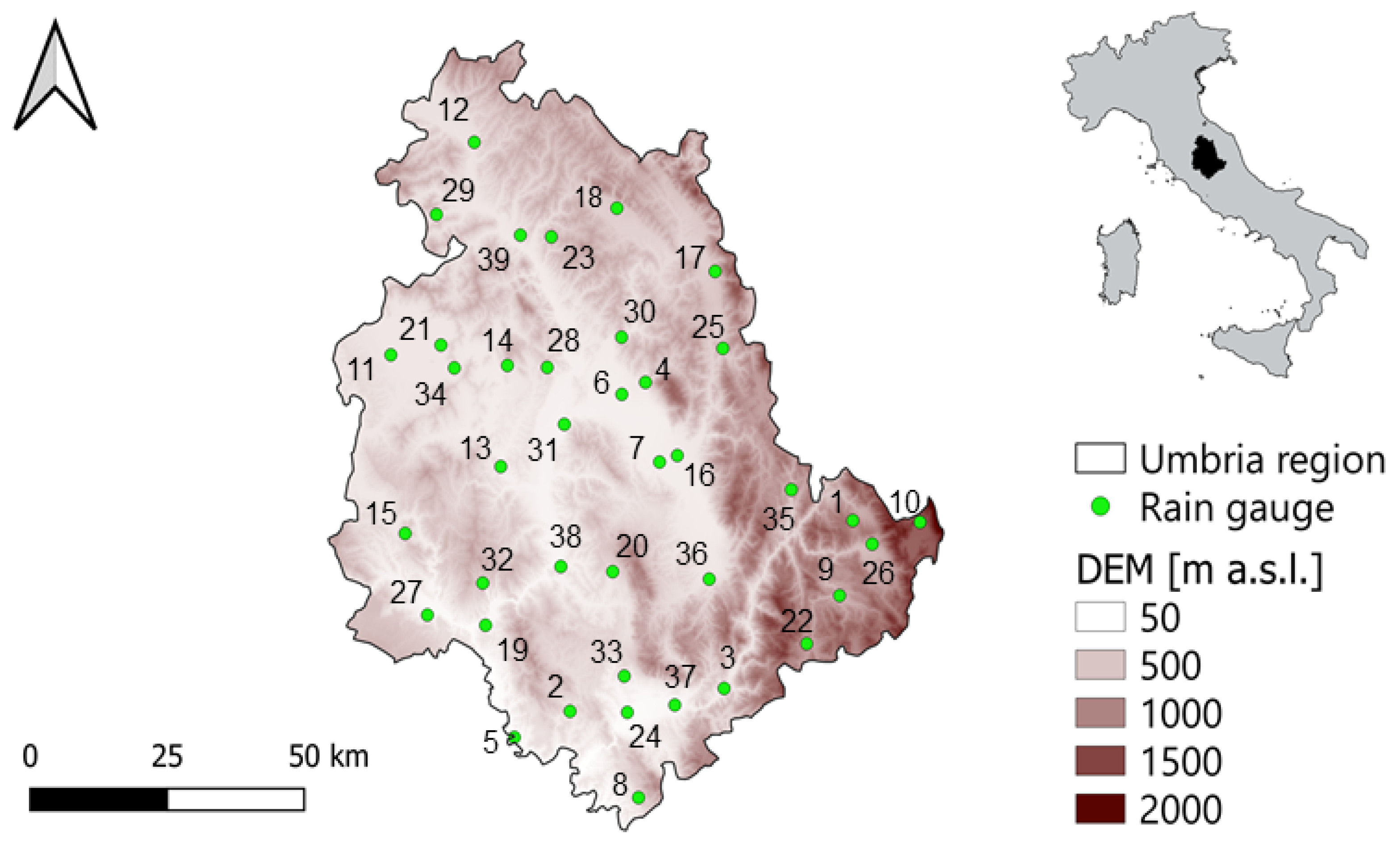
The study area (Umbria region, with a surface area of 8456 km2) is located in an inland zone of central Italy, and is characterized by a complex orography along the eastern boundary, where the Apennine Mountains exceed 2000 m a.s.l. In the central and western areas, orography is mainly of hilly type, with elevations ranging from 100 to 800 m a.s.l.. A wide percentage of the study area is included in the basin of Tiber River that crosses the region from north to south-west receiving water from many tributaries, mainly located on the hydrographic left side.
On the basis of observations made by the rain gauge network shown in Figure 1 and specified in Table 1, annual rainfall depth through the region ranges from 650 mm to 1450 mm, with mean value of about 900 mm. Higher monthly rainfall values generally occur during the autumn-winter period, with floods caused by widespread rainfall.
For each selected station, we considered all the Hd=24 h values already obtained and validated from the Regional Hydrographic Service (RHS) by using the available rainfall data. It is important to note that recently, mainly since 1992, it has been possible to obtain rainfall data recorded in data-loggers for each tip time associated with a fixed rainfall depth (no more than 0.2 mm). In this case, each rainfall event was summarized by aggregating the number of tips over a ta equal to 1 min. Nevertheless, for long time series, a considerable amount of rainfall data was available with hourly recording system, as a consequence of the paper rolls adoption. Furthermore, in the absence of other possibilities, daily information derived from direct observation made each day at 9:00 a.m. was used. Two examples of the Hd=24 h series used in this paper are shown in Table 2 and Table 3 for the Gubbio and Todi rain gauge stations, respectively. For all analyses carried out in this paper, 39 Hd=24 h time series for the rain gauge stations reported in Table 1 were selected.
3. Methods
Each of the selected Hd=24 h series, hereinafter referred to as “uncorrected” because they can contain some underestimated values (see also [47]), is used to verify the existence of possible trend produced by climate change. Specifically, we considered the following tests, selected as they are characterized by very different approaches: (1) least-squares linear trend analysis; (2) non-parametrical Mann–Kendall test [49,50]; and (3) Sen’s method [51].
The least-squares method uses a straight line in order to fit the given points and it is known as the method of linear or ordinary least squares. This line is found as the best fit from which the sum of squares of the distances from the points is minimized. Equations with certain parameters usually represent the results in this method. The method of least squares actually defines the solution for the minimization of the sum of squares of deviations or the errors in the result of each equation.
The non-parametrical Mann–Kendall test is commonly used in detecting trends of variables in many fields. Statistic S can be calculated by the following:
with:
and where n is the length of the sample, 𝑥k and 𝑥j are from 𝑘 = 1, 2, …, n − 1 and 𝑗 = 𝑘 + 1, …, n. If n is bigger than 8, statistic S approximates to normal distribution. The mean of S is 0 and the variance of S can be acquired as follows:
Then, the test statistic Z is denoted by:
If Z > 0, it indicates an increasing trend, and vice versa. Given a confidence level α, the sequential data would be supposed to experience statistically significant trend if |Z| > Z(1 − α/2), where Z(1 − α/2) is the corresponding value of P = α/2 following the standard normal distribution. In this study, a 0.05 confidence level was used.
Finally, the innovative trend analysis proposed by Sen (2012) is based on a sub-section time series plot on a Cartesian coordinate system. In this method, recently criticized by [52], a time series is divided into two equal parts that are separately sorted in ascending order. Then, the first sub-series is located on the X-axis, and the second sub-series is located on the Y-axis. If the investigated data are collected on the 1:1 line, then there is no trend. If data fall above the 1:1 line or below the 1:1 line, then an upward trend or a downward trend in the time series, respectively, exists [51].
We note that these three very common tests could be representative to many others. Furthermore, since they are characterized by very different approaches, they could potentially offer different results.
Successively, the above-mentioned tests were repeated on a new version of the same series (hereinafter referred to as “corrected”), where the underestimation error due to the coarse time resolution of historical rainfall data was eliminated/minimized by using an average correction identically applied to all Hd values characterized by the same ratio ta/d. We note that an alternative correction approach, based on a sophisticated stochastic method, would produce very similar results with respect to the simple deterministic approach used here [48]. Note that this last result cannot be easily generalized to any other analysis [10,53,54]. With the aim of applying the correction, the average underestimation errors, Ea%, have been determined through the relations proposed earlier by [47], expressed by:
4. Results and Discussion
As previously mentioned, initially the Hd=24 h series were corrected through the use of Equation (5c) proposed by [47]. For correction, we could use any of the relationships proposed by [36,37,38,39,40,41,42,43,44,45,46], but there is no reason to assume that this choice could have a significant effect on the results we present. As an example, Table 4 shows the Hd=24 h series of the Spoleto station, both in the original version (“uncorrected”) and in the “corrected” version.
Then, we fitted a least-squares linear trend to the Hd=24 h in both versions, “uncorrected” and “corrected”, considering all 39 selected stations. For the “uncorrected” Hd=24 h series, the number of positive least-square linear trends, equal to 23, outnumbers the negative ones, equal to 16 (see also Table 5). Opposite results were obtained for the “corrected” Hd=24 h series, as cases with negative least-square linear trends become equal to 27, whereas the positive ones become 12.
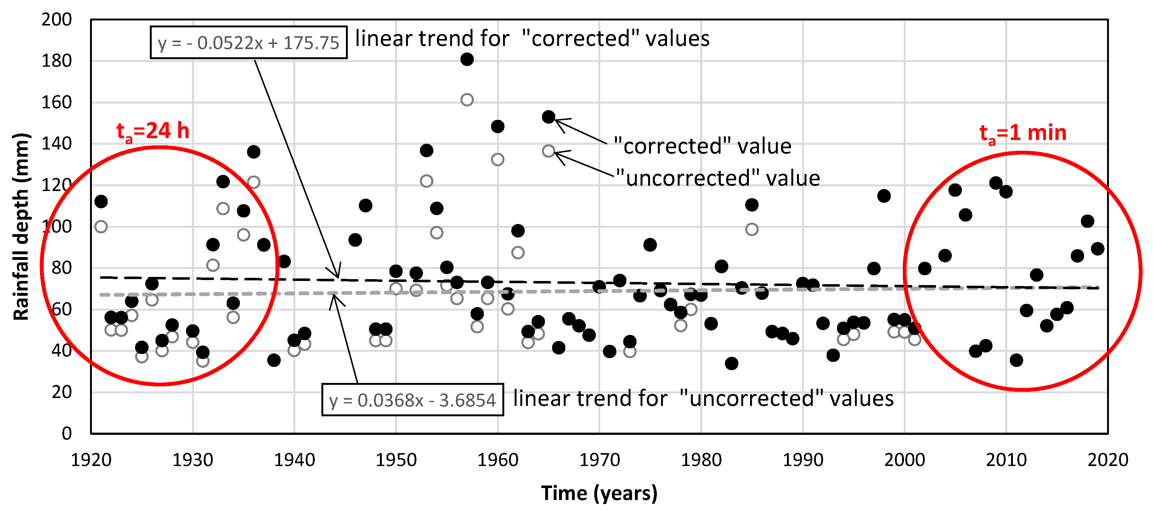
Figure 2 shows a comparison between “uncorrected” and “corrected” annual maximum rainfall depths for duration 24 h regarding Terni station. As can be seen, the “uncorrected” series shows a positive trend, while the “corrected” series linear trend is negative. This is mainly due to the fact that many old Hd=24 h values were underestimated, due to being derived by daily observations, while in the last decades the original Hd=24 h values have been determined without errors by using rainfall data recorded in data-loggers for each tip time associated with a fixed rainfall depth equal to 0.1 or 0.2 mm. Then, from a geometric point of view, if older values increase due to corrections and the most recent ones remain unchanged, the linear regression will be characterized by a decreasing slope.
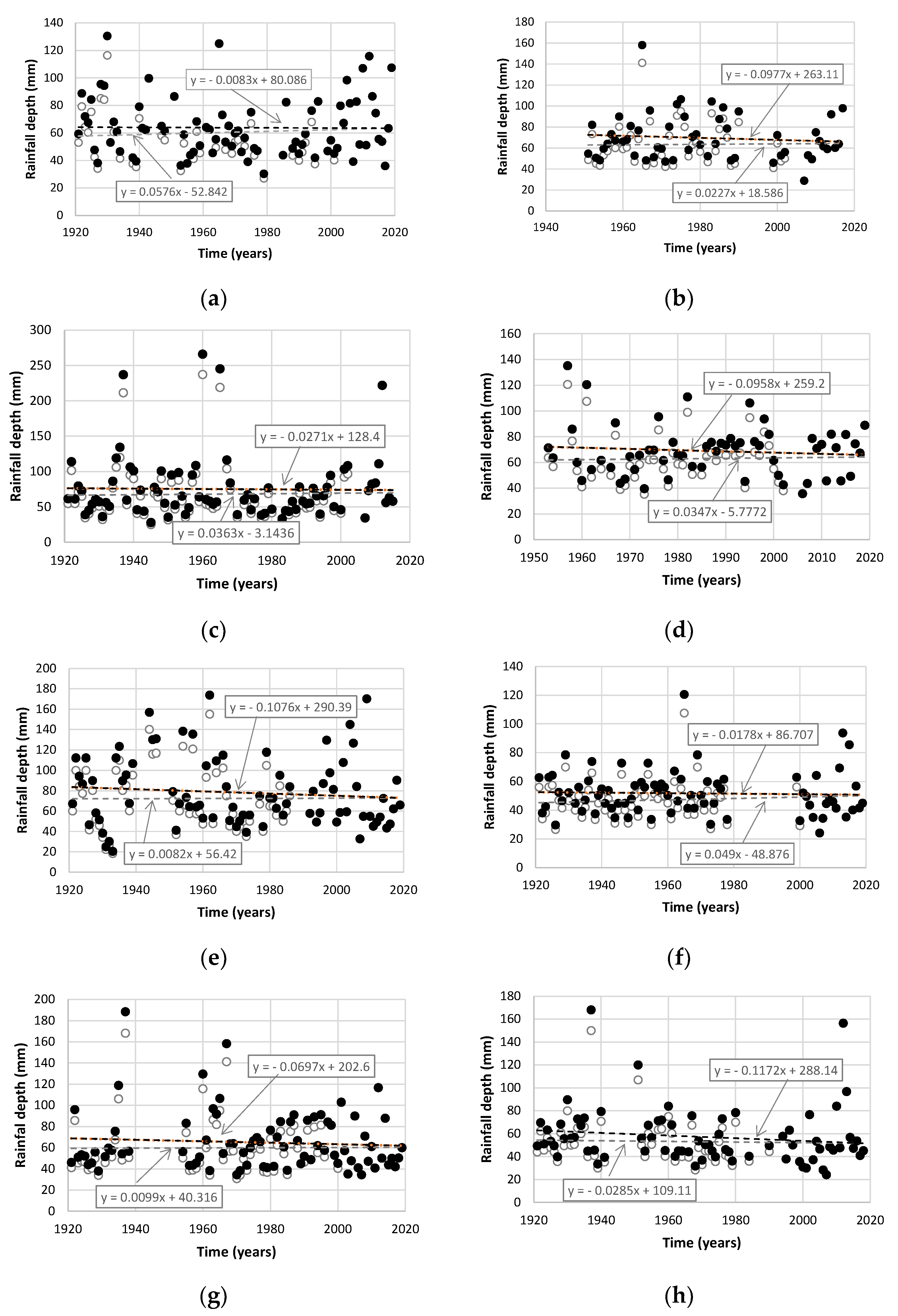
Figure 3 shows the same comparison of Figure 2 between “uncorrected” and “corrected” Hd=24 h series for a restricted number of representative stations. It can be seen that, in some cases, such as that of Figure 3h regarding San Savino station, the least-square linear trend was also negative before correction with Equation (5c), with slope of the linear regression equal to −0.0285 mm/year. However, after correction, the negative trend becomes exacerbated (slope of the linear regression equal to −0.1172 mm/year).
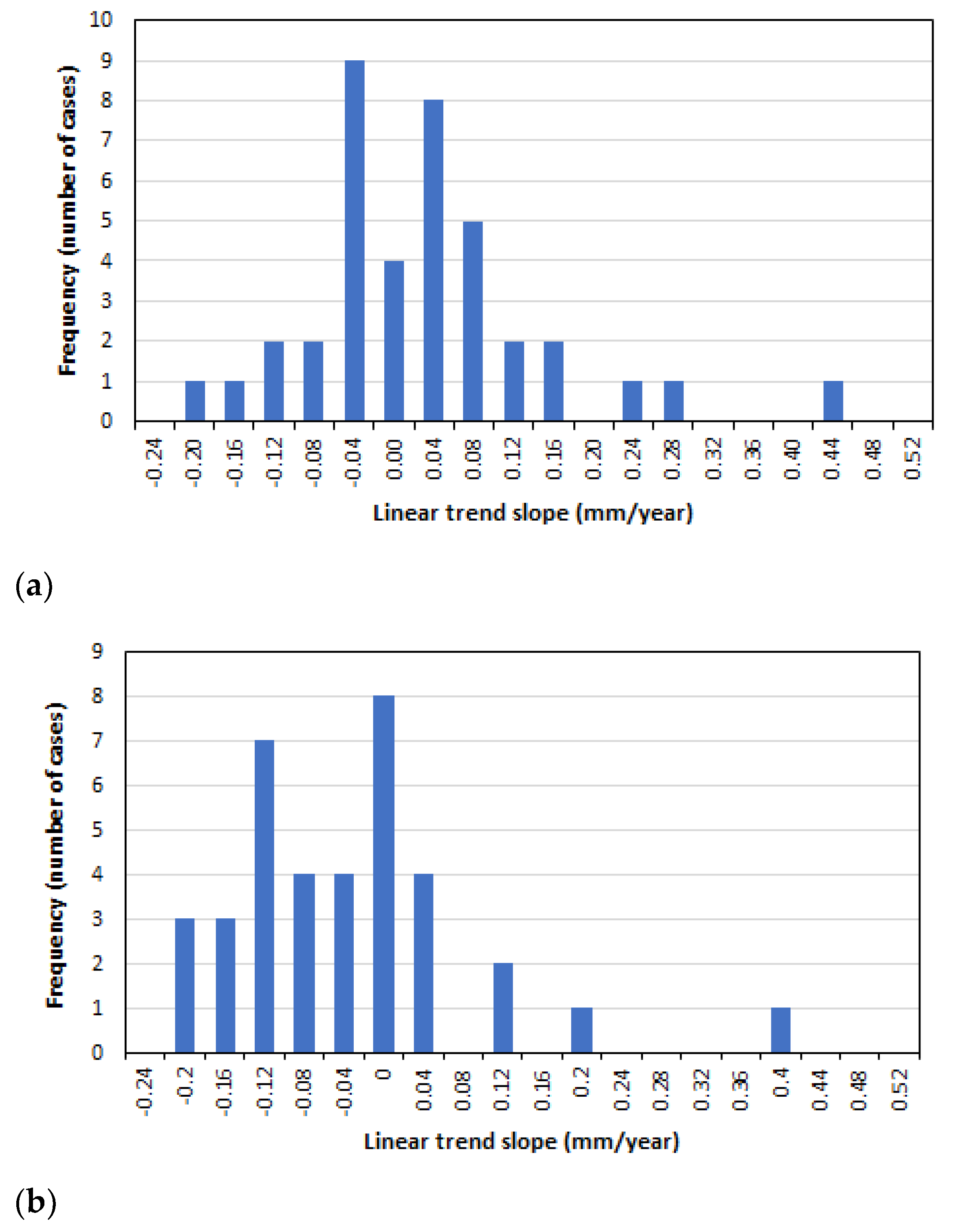
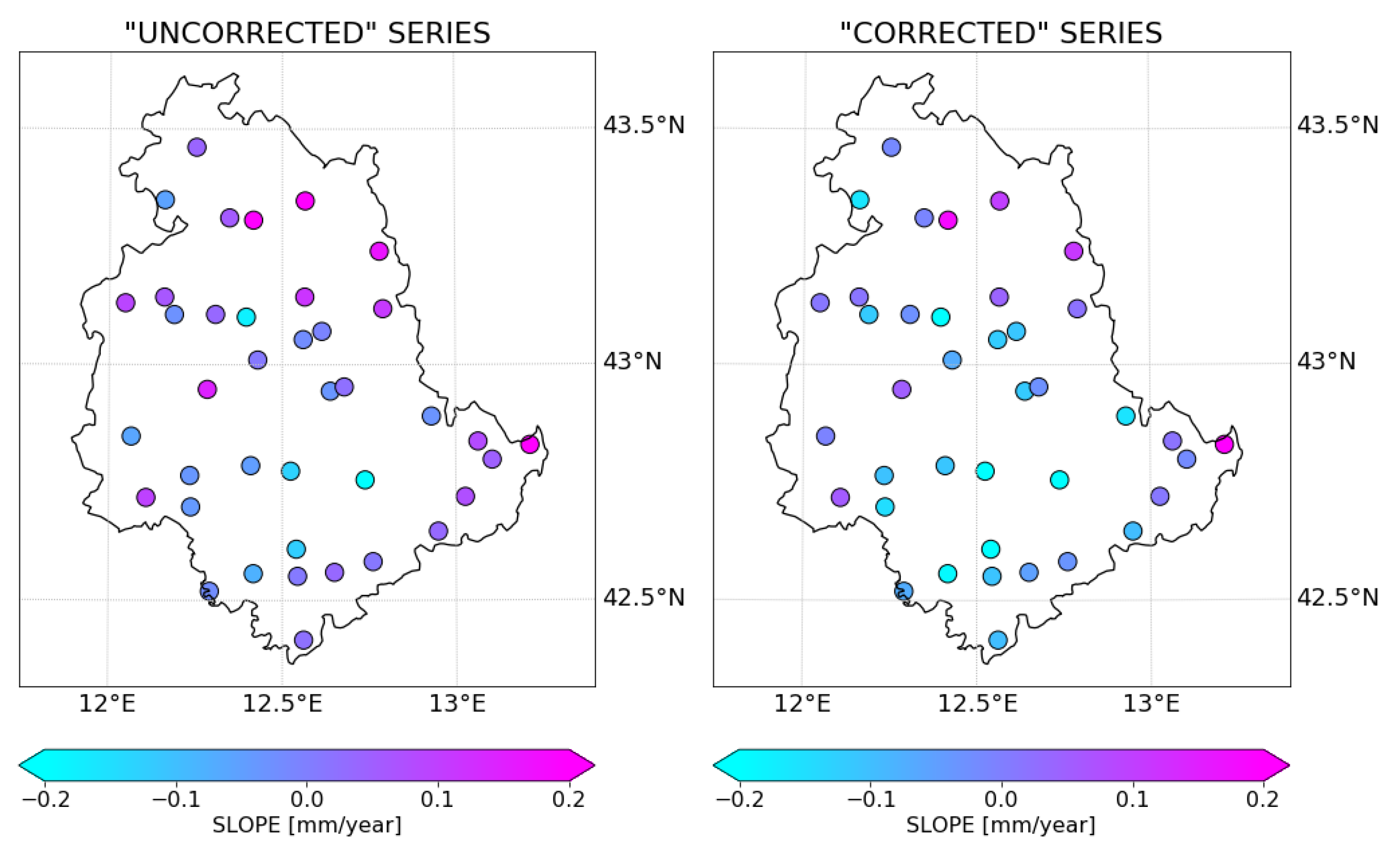
With the main purpose to obtain useful and intuitive graphic representations of the linear trend slopes for both “uncorrected” and “corrected” series, Figure 4 shows the frequency of a reasonable number of slope classes, while in Figure 5 positive and negative slope values have been located in the geographic position of each rain gauge station.
Figure 4 highlights that a Gaussian probability function could be adequate to represent the distribution of linear trend slope values independently if “uncorrected” or “corrected” series are considered, with the average value changing from positive (0.0287) in the case of the “uncorrected” series to negative (−0.0485) for the “corrected” series. As it can also be deduced in Table 5, the two standard deviations are almost indistinguishable.
Figure 5 highlights that, within the Umbria region, there are no geographic areas most affected by specific trends, both when considering the “uncorrected” or “corrected” series.
The analysis of the 39-time series was successively performed by the non-parametric Mann–Kendall test. For the “uncorrected” series, by using a significance level equal to 0.05, the percentage without significant trends is approximately 90%, with one series (Spoleto) characterized by a significant negative trend, and three series (Castelluccio di Norcia, Gubbio and Montelovesco) by a significant positive trend (see Table 5). After the correction, the Mann–Kendall test evidenced six cases with a significant negative trend (Abeto, Massa Martana, Perugia, San Gemini, San Savino and Spoleto), and no positive cases. Therefore, for the Mann–Kendall test, the transition from “uncorrected” and “corrected” Hd=24 h series produces different results and conclusions.
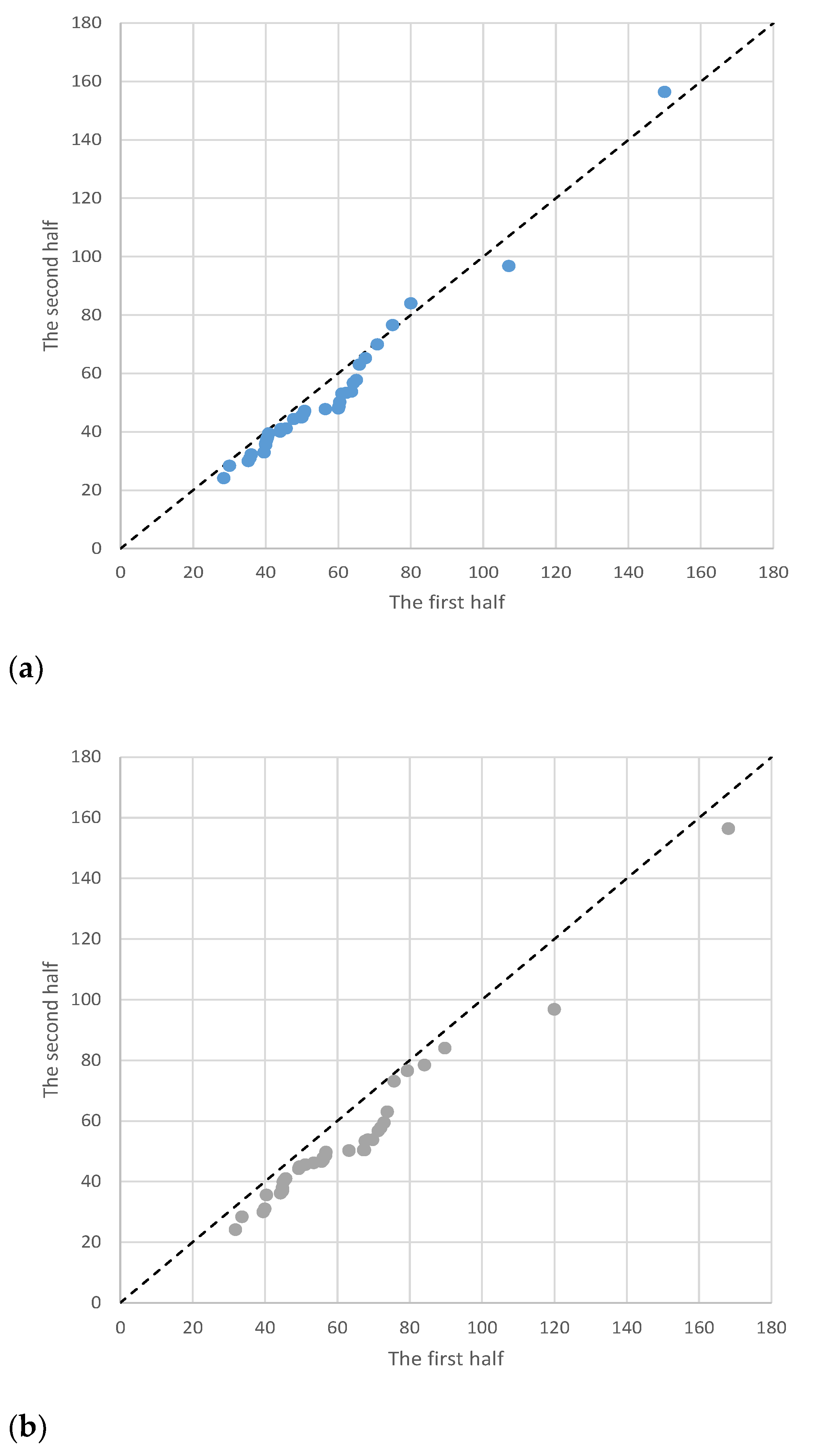
Similarly to that which has already emerged using the most classic analyses, Sen’s method also produces different results when applied to the “uncorrected” and “corrected” annual maximum rainfall depths series. As an example, Figure 6 shows the results of the method for both the “uncorrected” and “corrected” Hd=24 h series observed at San Savino station. As can be seen in Figure 6a, the “uncorrected” series shows a no trend condition, because all values are close to 1:1 line and cross it several times, while in Figure 6b, the “correct” series evidences a clear monotonic decreasing trend (details on the results interpretation can be found in [51]).
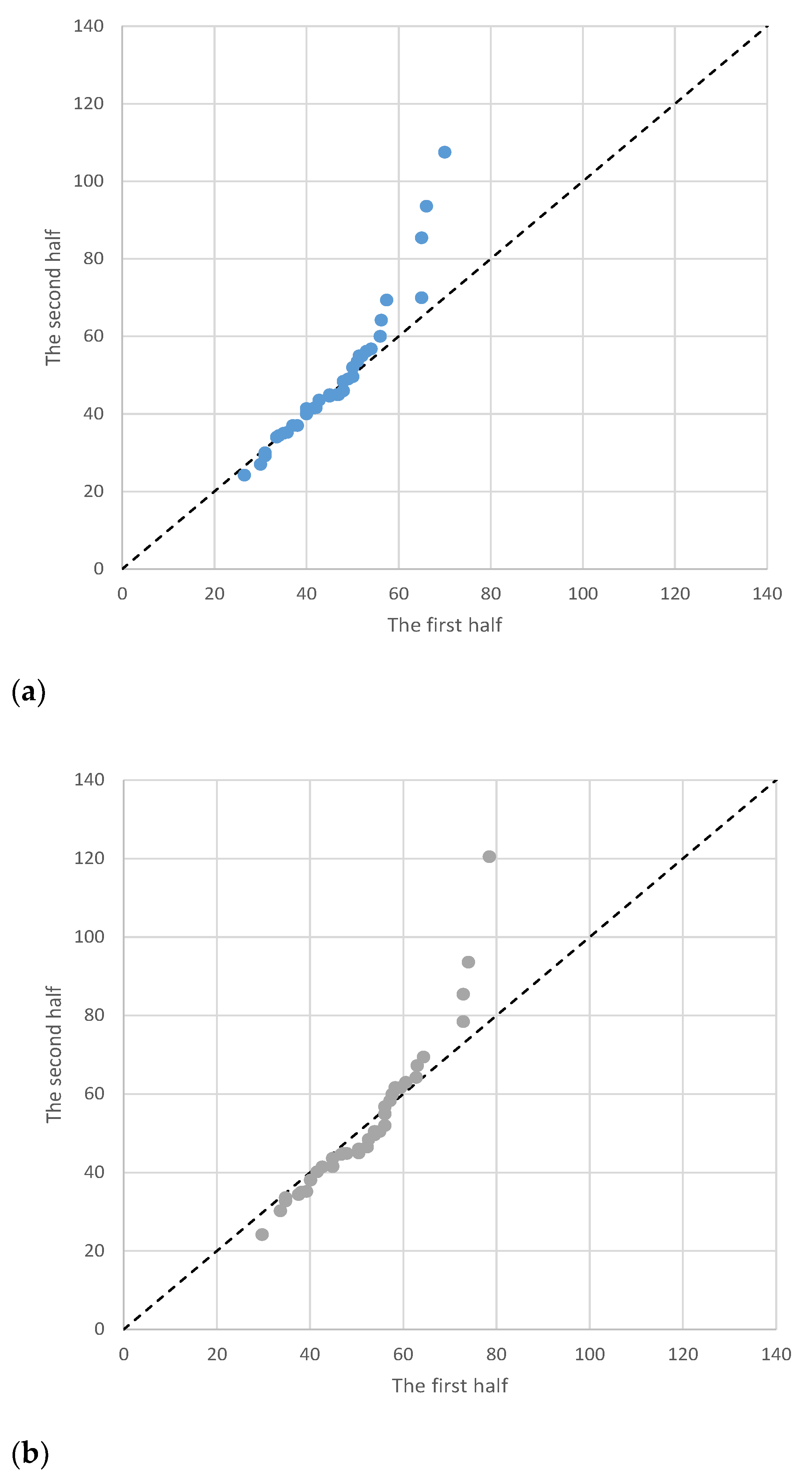
It is interesting to note Sen’s method appears less sensitive to the Hd underestimation, due to the rainfall coarse temporal aggregation than classical linear regression and Mann–Kendall methods. This depends by the graphical approach on which the method is based. The example of the series regarding Norcia station is emblematic. Moving from the “uncorrected” series to the “corrected” series, both the linear trend slope and the Mann–Kendall test statistic Z change from positive to negative values (see Table 5). Instead, as shown in Figure 7, Sen’s method suggests that both “uncorrected” and “corrected” series are non-monotonically increasing.
All the results we have presented refer to a region of central Italy. We believe that they can be generalized to any other geographical area of the world, since it is widely demonstrated that the problem of the Hd underestimation is dependent on the technological evolution of rainfall recording systems, with all places showing similarity. In any case, we hope that this work can stimulate other case studies.
Even outside of the scope of this paper, it can be stated that, recently, in a study region located in central Italy, extreme rainfall events characterized by duration 24 h have not clearly and significantly deviated to trends observed 50–80 years ago. Therefore, despite in this region the effects of climate change having produced a continuous decrease in the annual rainfall amount and a significant increase of annual and monthly air temperature, these proclamations that try to attribute to climatic changes also the responsibility for the worrying hydrological and geological instability of the regional territory are not at all justified.
5. Conclusions
In the scientific literature, it is possible to find many analyses conducted to assess whether climate change has influenced the trends of the annual maximum rainfall depths with a duration of 24 h. Although it is well known that the Hd values obtained from rainfall data characterized by coarse temporal resolution can be significantly underestimated, the aforementioned analyses have been always conducted without taking into account the data origin.
The main objective of this paper was to evaluate the effect of time-resolution of rainfall data on Hd=24 h series trend estimation.
A representative number of rain gauge stations working perfectly for approximately a century with available Hd=24 h series, validated by the Regional Hydrographic Service, was carefully chosen.
All selected series, referred to as “uncorrected” since there were certainly some data containing some underestimated values [47], were used to verify the existence of possible trend due to climate change. For this purpose, we considered the very common least-squares linear trend analysis, the non-parametrical Mann–Kendall test, and the Sen’s method. Successively, the same series were modified through the procedure proposed by [47], with the purpose of eliminating/minimizing the underestimations, obtaining the so-called “corrected” series.
The underestimation errors due to coarse time-resolution of rainfall data produce significant effects on the least-squares linear trend analysis (based on a geometric approach) of the Hd=24 h values. Specifically, since a prevalence of increasing and decreasing trends for “uncorrected” and “corrected” series, respectively, was observed, the correction procedure can change the sign of the trend. For the non-parametric Mann–Kendall test (based on a statistical approach) with a significance level 0.05, using the selected 39 “uncorrected” time series, only one case was characterized by a significant negative trend, while three cases exhibited a significant positive trend. After the corrections, cases with negative trends became six, and there were no cases with a positive trend. Finally, the innovative Sen’s method (based on a graphical approach) has been noted to be less sensitive to corrections of the Hd values than the least-squares linear trend and the Mann–Kendall method. However, its results on the Hd=24 h series were also affected by the correction.
Overall, it can be concluded that the analysis of Hd series containing potentially underestimated values, especially when d = 24 h, can lead to misleading results. Therefore, before conducting any trend analysis, Hd values determined from rainfall data characterized by coarse temporal resolution should always be corrected with appropriate procedures suggested by the scientific literature. This correction could be neglected in the analysis performed by using the temporal scale of rainfall records [55].
The analysis conducted in this work may have the limit of considering rainfall data from only one geographical area of the world. There is no reason to assume that choosing only the case study of Umbria instead of many different case studies could have a significant effect on the results we presented. In any case, in the future we hope to find in the scientific literature similar analyses from many other territories.
Author Contributions
Investigation, writing—original draft preparation and writing—review and editing, R.M., C.S., J.D., A.F. All authors have read and agreed to the published version of the manuscript.
Funding
This research was mainly financed by University of Perugia (Fondo Ricerca di Base 2019).
Informed Consent Statement
Not applicable.
Data Availability Statement
The data presented in this study are available on request from the corresponding author.
Conflicts of Interest
The authors declare no conflict of interest.
References
- Koutsoyiannis, D. Revisiting the global hydrological cycle: Is it intensifying? Hydrol. Earth Syst. Sci. 2020, 24, 3899–3932. [Google Scholar] [CrossRef]
- Barnett, T.P.; Pierce1, D.W.; Hidalgo, H.G.; Bonfils, C.; Santer, B.D.; Das, T.; Bala, G.; Wood, A.W.; Nozawa, T.; Mirin, A.A.; et al. Human-induced changes in the hydrology of the Western United States. Science 2008, 319, 1080–1083. [Google Scholar] [CrossRef] [PubMed] [Green Version]
- Sharafati, A.; Pezeshki, E. A strategy to assess the uncertainty of a climate change impact on extreme hydrological events in the semi-arid Dehbar catchment in Iran. Theor. Appl. Climatol. 2020, 139, 389–402. [Google Scholar] [CrossRef]
- Hajani, E. Climate change and its influence on design rainfall at-site in new south wales state, Australia. J. Water Clim. Chang. 2020, 11, 251–269. [Google Scholar] [CrossRef]
- Homsi, R.; Sanusi Shiru, M.; Shahid, S.; Ismail, T.; Bin Harun, S.; Al-Ansari, N.; Chau, K.-W.; Mundher Yaseen, Z. Precipitation projection using a CMIP5 GCM ensemble model: A regional investigation of Syria. Eng. Appl. Comp. Fluid Mech. 2020, 14, 90–106. [Google Scholar] [CrossRef]
- IPCC. Global Warming of 1.5 °C. An IPCC Special Report on the Impacts of Global Warming of 1.5 °C above Pre-Industrial Levels and Related Global Greenhouse Gas Emission Pathways, in the Context of Strengthening the Global Response to the Threat of Climate Change, Sustainable Development, and Efforts to Eradicate Poverty; Masson-Delmotte, V., Zhai, P., Pörtner, H.-O., Roberts, D., Skea, J., Shukla, P.R., Pirani, A., Moufouma-Okia, W., Péan, C., Pidcock, R., et al., Eds.; World Meteorological Organization: Geneva, Switzerland, 2018; p. 32. [Google Scholar]
- Lenderink, G.; Van Meijgarrd, E. Increase in hourly precipitation extremes beyond expectations from temperature changes. Nat. Geosci. 2008, 1, 511–514. [Google Scholar] [CrossRef]
- Hardwick-Jones, R.; Westra, S.; Sharma, A. Observed relationships between extreme sub-daily precipitation, surface temperature, and relative humidity. Geophys. Res. Lett. 2010, 37, L22805. [Google Scholar] [CrossRef] [Green Version]
- Wang, J.-W.; Wang, K.; Pielke Sr, R.A.; Lin, J.C.; Matsui, T. Towards a robust test on North America warming trend and precipitable water content increase. Geophys. Res. Lett. 2008, 35, L18804. [Google Scholar] [CrossRef] [Green Version]
- Dimitriadis, P.; Koutsoyiannis, D.; Iliopoulou, T.; Papanicolaou, P. A global-scale investigation of stochastic similarities in marginal distribution and dependence structure of key hydrological-cycle processes. Hydrology 2021, 8, 59. [Google Scholar] [CrossRef]
- Kunkel, K. North American trends in extreme precipitation. Nat. Hazards 2003, 29, 291–305. [Google Scholar] [CrossRef]
- Re, M.; Barros, V.R. Extreme rainfalls in SE South America. Clim. Chang. 2009, 96, 119–136. [Google Scholar] [CrossRef]
- Fowler, H.J.; Ali, H. Changes in Extreme Rainfall Events under the Warming Climate. In Rainfall. Modeling, Measurement and Applications; Morbidelli, R., Ed.; Elsevier: Amsterdam, The Netherlands, 2021. [Google Scholar] [CrossRef]
- Sun, Q.; Zhang, X.; Zwiers, F.; Westra, S.; Alexander, L.V. A global, continental, and regional analysis of changes in extreme precipitation. J. Clim. 2021, 34, 243–258. [Google Scholar] [CrossRef]
- Guerreiro, S.B.; Fowler, H.J.; Barbero, R.; Westra, S.; Lenderink, G.; Blenkinsop, S.; Li, X.F. Detection of continental-scale intensification of hourly rainfall extremes. Nat. Clim. Chang. 2018, 8, 803–807. [Google Scholar] [CrossRef]
- Roxy, M.K.; Ghosh, S.; Pathak, A.; Athulya, R.; Mujumdar, M.; Murtugudde, R.; Rajeevan, M. A threefold rise in widespread extreme rain events over central India. Nat. Commun. 2017, 8, 1–11. [Google Scholar] [CrossRef] [PubMed]
- Wang, Y.; Zhou, L. Observed trends in extreme precipitation events in China during 1961–2001 and the associated changes in large-scale circulation. Geophys. Res. Lett. 2005, 32, L09707. [Google Scholar] [CrossRef]
- Shahid, S. Trends in extreme rainfall events of Bangladesh. Theor. Appl. Climatol. 2011, 104, 489–499. [Google Scholar] [CrossRef]
- Park, J.S.; Kang, H.S.; Lee, Y.S.; Kim, M.K. Changes in the extreme daily rainfall in South Korea. Int. J. Climatol. 2011, 31, 2290–2299. [Google Scholar] [CrossRef]
- Nkrumah, F.; Vischel, T.; Panthou, G.; Klutse, N.A.B.; Adukpo, D.C.; Diedhiou, A. Recent trends in the daily rainfall regime in southern West Africa. Atmosphere 2019, 10, 741. [Google Scholar] [CrossRef] [Green Version]
- Donat, M.G.; Alexander, L.V.; Herold, N.; Dittus, A.J. Temperature and precipitation extremes in century-long gridded observations, reanalyses, and atmospheric model simulations. J. Geophys. Res. Atmos. 2016, 121, 11174–11189. [Google Scholar] [CrossRef] [Green Version]
- Gershunov, A.; Cayan, D.R. Heavy daily precipitation frequency over the contiguous United States: Sources of climatic variability and seasonal predictability. J. Clim. 2003, 16, 2752–2765. [Google Scholar] [CrossRef] [Green Version]
- Schreck, C.J.; Semazzi, F.H.M. Variability of the recent climate of Eastern Africa. Int. J. Climatol. 2004, 24, 681–701. [Google Scholar] [CrossRef]
- Grimm, A.M.; Tedeschi, R.G. ENSO and extreme rainfall events in South America. J. Clim. 2009, 22, 1589–1609. [Google Scholar] [CrossRef]
- Haylock, M.R.; Peterson, T.C.; Alves, L.M.; Ambrizzi, T.; Anunciação, Y.M.T.; Baez, J.; Barroz, V.R.; Berlato, M.A.; Bidegain, M.; Coronel, G.; et al. Trends in total and extreme South America rainfall in 1960–2000 and links with sea surface temperature. J. Clim. 2006, 19, 1490–1512. [Google Scholar] [CrossRef]
- Cayan, D.R.; Redmond, K.T.; Riddle, L.G. ENSO and hydrologic extremes in the western United States. J. Clim. 1999, 12, 2881–2893. [Google Scholar] [CrossRef] [Green Version]
- Gershunov, A. ENSO influence on intraseasonal extreme rainfall and temperature frequencies in the contiguous United States: Implications for long-range predictability. J. Clim. 1998, 11, 3192–3203. [Google Scholar] [CrossRef]
- Aryal, S.K.; Bates, B.C.; Campbell, E.P.; Li, Y.; Palmer, M.J.; Viney, N.R. Characterizing and modelling temporal and spatial trends in rainfall extremes. J. Hydromet. 2009, 10, 241–253. [Google Scholar] [CrossRef]
- Kamruzzaman, M.; Beecham, S.; Metcalfe, A.V. Non-stationarity in rainfall and temperature in the Murray Darling Basin. Hydrol. Proc. 2011, 25, 1659–1675. [Google Scholar] [CrossRef]
- Kendon, E.J.; Blenkinsop, S.; Fowler, H.J. Will changes in short duration precipitation extremes be detectable before daily extremes? J. Clim. 2018, 31. [Google Scholar] [CrossRef]
- Willems, P. Adjustment of extreme rainfall statistics accounting for multidecadal climate oscillations. J. Hydrol. 2013, 490, 126–133. [Google Scholar] [CrossRef]
- Teegavarapu, R.S.V.; Nayak, A. Evaluation of long-term trends in extreme precipitation: Implications of in-filled historical data use for analysis. J. Hydrol. 2017, 550, 616–634. [Google Scholar] [CrossRef]
- Bonaccorso, B.; Cancelliere, A.; Rossi, G. Detecting trends of extreme rainfall series in Sicily. Adv. Geosci. 2005, 2, 7–11. [Google Scholar] [CrossRef] [Green Version]
- Fatichi, S.; Caporali, E. A comprehensive analysis of changes in precipitation regime in Tuscany. Int. J. Climatol. 2009, 29, 1883–1893. [Google Scholar] [CrossRef]
- Morbidelli, R.; García-Marín, A.P.; Al Mamun, A.; Atiqur, R.M.; Ayuso-Muñoz, J.L.; Bachir Taouti, M.; Baranowski, P.; Bellocchi, G.; Sangüesa-Pool, C.; Bennett, B.; et al. The history of rainfall data time-resolution in different geographical areas of the world. J. Hydrol. 2020, 590, 125258. [Google Scholar] [CrossRef]
- Hershfield, D.M.; Wilson, W.T. Generalizing of Rainfall-intensity-frequency Data. IUGG/IAHS Publication No. 43; AIHS. Gen. Ass. Tor. 1958, 1, 499–506. [Google Scholar]
- Hershfield, D.M. Rainfall Frequency Atlas of the United States for Durations from 30 Minutes to 24 Hours and Return Periods from 1 to 100 Years; US Weather Bureau Technical Paper N. 40; U.S. Department of Commerce: Washington, DC, USA, 1961. [Google Scholar]
- Weiss, L.L. Ratio of true to fixed-interval maximum rainfall. J. Hydraul. Div. 1964, 90, 77–82. [Google Scholar] [CrossRef]
- Harihara, P.S.; Tripathi, N. Relationship of the clock-hour to 60-min and the observational day to 1440-min rainfall. Ind. J. Meteorol. Geophys. 1973, 24, 279–282. [Google Scholar]
- Natural Environment Research Council. Flood Studies Report; Natural Environmental Research Council: London, UK, 1975. [Google Scholar]
- Van Montfort, M.A.J. Sliding maxima. J. Hydrol. 1990, 118, 77–85. [Google Scholar] [CrossRef]
- Faiers, G.E.; Grymes, J.M.; Keim, B.D.; Muller, R.A. A re-examination of extreme 24 hour rainfall in Louisiana, USA. Clim. Res. 1994, 4, 25–31. [Google Scholar] [CrossRef]
- Van Montfort, M.A.J. Concomitants of the Hershfield factor. J. Hydrol. 1997, 194, 357–365. [Google Scholar] [CrossRef]
- Young, C.B.; McEnroe, B.M. Sampling adjustment factors for rainfall recorded at fixed time intervals. J. Hydrol. Eng. 2003, 8, 294–296. [Google Scholar] [CrossRef]
- Yoo, C.; Park, M.; Kim, H.J.; Choi, J.; Sin, J.; Jun, C. Classification and evaluation of the documentary-recorded storm events in the Annals of the Choson Dynasty (1392–1910), Korea. J. Hydrol. 2015, 520, 387–396. [Google Scholar] [CrossRef]
- Papalexiou, S.M.; Dialynas, Y.G.; Grimaldi, S. Hershfield factor revisited: Correcting annual maximum precipitation. J. Hydrol. 2016, 524, 884–895. [Google Scholar] [CrossRef]
- Morbidelli, R.; Saltalippi, C.; Flammini, A.; Cifrodelli, M.; Picciafuoco, T.; Corradini, C.; Casas-Castillo, M.C.; Fowler, H.J.; Wilkinson, S.M. Effect of temporal aggregation on the estimate of annual maximum rainfall depths for the design of hydraulic infrastructure systems. J. Hydrol. 2017, 554, 710–720. [Google Scholar] [CrossRef] [Green Version]
- Morbidelli, R.; Saltalippi, C.; Flammini, A.; Corradini, C.; Wilkinson, S.M.; Fowler, H.J. Influence of temporal data aggregation on trend estimation for intense rainfall. Adv. Water. Resour. 2018, 122, 304–316. [Google Scholar] [CrossRef]
- Mann, H.B. Nonparametric tests against trend. Econometrica 1945, 13, 46–59. [Google Scholar] [CrossRef]
- Kendall, M.G. Rank Correlation Methods; Griffin: London, UK, 1975. [Google Scholar]
- Sen, Z. Innovative trend analysis methodology. J. Hydrol. Eng. 2012, 17, 1042–1046. [Google Scholar] [CrossRef]
- Serinaldi, F.; Chebana, F.; Kilsby, C.G. Dissecting innovative trend analysis. Stoch. Environ. Res. Risk Assess. 2020, 34, 733–754. [Google Scholar] [CrossRef]
- Iliopoulou, T.; Koutsoyiannis, D. Revealing hidden persistence in maximum rainfall records. Hydrol. Sci. J. 2019, 64, 1673–1689. [Google Scholar] [CrossRef]
- Iliopoulou, T.; Koutsoyiannis, D. Projecting the future of rainfall extremes: Better classic than trendy. J. Hydrol. 2020, 588. [Google Scholar] [CrossRef]
- Koutsoyiannis, D. Stochastics of Hydroclimatic Extremes—A Cool Look at Risk; Kallipos: Athens, Greece, 2021; 333p, ISBN 978-618-85370-0-2. [Google Scholar]
Figure 1.
Morphology of the study area and rain gauges used in the analysis with identification numbers listed in Table 1. The background Digital Elevation Model (DEM), whose spatial resolution is 25 m, is derived by the Copernicus EU-DEM v1.1.
Figure 1.
Morphology of the study area and rain gauges used in the analysis with identification numbers listed in Table 1. The background Digital Elevation Model (DEM), whose spatial resolution is 25 m, is derived by the Copernicus EU-DEM v1.1.

Figure 2.
Time sequence of “uncorrected” and “corrected” annual maximum rainfall depths for duration 24 h, Hd=24 h, with the respective linear trends, for Terni station. The red circles highlight periods where the Hd=24 h values have been obtained from rainfall data with the indicated aggregation time, ta. During the period 1936–2001 Hd=24 h values have been obtained from rainfall data with variable ta. Available data within the period 1921–2019.

Figure 3.
Time sequence of “uncorrected” and “corrected” annual maximum rainfall depths for duration 24 h, Hd=24 h, with the respective linear trends, for the following stations: (a) Umbertide; (b) Calvi dell’Umbria; (c) Ficulle; (d) Monteleone di Spoleto; (e) Narni Scalo; (f) Norcia; (g) Ponte Nuovo; and (h) San Savino. Available data within the period 1921–2019.

Figure 4.
Frequency of the linear trend slope for (a) “uncorrected” and (b) “corrected” Hd=24 h series considering classes amplitude equal to 0.04 mm/year. All selected rain gauge stations were considered.
Figure 4.
Frequency of the linear trend slope for (a) “uncorrected” and (b) “corrected” Hd=24 h series considering classes amplitude equal to 0.04 mm/year. All selected rain gauge stations were considered.

Figure 5.
Values of the linear trend slopes for both “uncorrected” (left) and “corrected” (right) Hd=24 h series located in the corresponding geographic position of the rain gauge station.
Figure 5.
Values of the linear trend slopes for both “uncorrected” (left) and “corrected” (right) Hd=24 h series located in the corresponding geographic position of the rain gauge station.

Figure 6.
Trend conditions according to Sen’s method for the annual maximum rainfall depths for San Savino station and duration equal to 24 h: (a) “uncorrected” series; and (b) “corrected” series. Available data within the period 1921–2018.
Figure 6.
Trend conditions according to Sen’s method for the annual maximum rainfall depths for San Savino station and duration equal to 24 h: (a) “uncorrected” series; and (b) “corrected” series. Available data within the period 1921–2018.

Figure 7.
Trend conditions according to Sen’s method for the annual maximum rainfall depths for Norcia station and duration equal to 24 h: (a) “uncorrected” series; and (b) “corrected” series. Available data within the period 1921–2019.
Figure 7.
Trend conditions according to Sen’s method for the annual maximum rainfall depths for Norcia station and duration equal to 24 h: (a) “uncorrected” series; and (b) “corrected” series. Available data within the period 1921–2019.


Table 1.
Main characteristics of the selected rainfall stations. The geographic position is expressed in Universal Transvers Mercator (UTM) coordinates computed by using the WGS84 ellipsoid model. ARDta is the percentage of available rainfall data characterized by specific temporal aggregation, ta.
Table 1.
Main characteristics of the selected rainfall stations. The geographic position is expressed in Universal Transvers Mercator (UTM) coordinates computed by using the WGS84 ellipsoid model. ARDta is the percentage of available rainfall data characterized by specific temporal aggregation, ta.
| ID Number | Rain Gauge Station | Altitude (m a.s.l.) | UTM33 X (m) | UTM33 Y (m) | Available Data Period | ARDta (%) | ||
|---|---|---|---|---|---|---|---|---|
| ta = 1 min | ta = 60 min | ta = 1440 min | ||||||
| 1 | Abeto | 946 | 341,805 | 4,744,571 | 1951–2014 | 9.4 | 0.0 | 90.6 |
| 2 | Amelia | 321 | 287,959 | 4,714,829 | 1921–2017 | 19.2 | 20.5 | 60.3 |
| 3 | Arrone | 221 | 316,289 | 4,716,860 | 1921–2017 | 11.0 | 0.0 | 89.0 |
| 4 | Assisi | 408 | 305,799 | 4,771,442 | 1921–2001 | 0.0 | 45.2 | 54.8 |
| 5 | Attigliano | 64 | 277,495 | 4,711,022 | 1921–2015 | 11.8 | 0.0 | 88.2 |
| 6 | Bastia | 203 | 301,377 | 4,769,716 | 1922–2017 | 31.8 | 0.0 | 68.2 |
| 7 | Bevagna | 212 | 307,370 | 4,757,320 | 1921–2017 | 21.7 | 6.0 | 72.3 |
| 8 | Calvi dell’Umbria | 305 | 299,164 | 4,698,561 | 1951–2017 | 20.4 | 0.0 | 79.6 |
| 9 | Cascia | 604 | 338,477 | 4,731,592 | 1922–2017 | 19.6 | 0.0 | 80.4 |
| 10 | Castelluccio di Norcia | 1349 | 354,031 | 4,743,409 | 1921–2017 | 12.7 | 0.0 | 87.3 |
| 11 | Castiglione del Lago | 260 | 259,760 | 4,779,579 | 1921–2019 | 15.7 | 27.1 | 57.1 |
| 12 | Città di Castello | 304 | 277,643 | 4,815,738 | 1921–2019 | 36.4 | 29.9 | 33.8 |
| 13 | Compignano | 240 | 278,394 | 4,758,593 | 1922–2017 | 34.6 | 0.0 | 65.4 |
| 14 | Corciano | 306 | 280,871 | 4,776,204 | 1921–2019 | 16.4 | 0.0 | 83.6 |
| 15 | Ficulle | 440 | 260,144 | 4,747,480 | 1921–2015 | 10.8 | 0.0 | 89.2 |
| 16 | Foligno | 220 | 310,678 | 4,758,225 | 1916–2015 | 25.7 | 31.4 | 42.9 |
| 17 | Gualdo Tadino | 599 | 319,870 | 4,789,953 | 1921–2019 | 18.4 | 47.1 | 34.5 |
| 18 | Gubbio | 471 | 302,789 | 4,802,329 | 1921–2019 | 20.0 | 42.5 | 37.5 |
| 19 | Lago di Corbara | 128 | 273,640 | 4,731,014 | 1963–2019 | 34.0 | 0.0 | 66.0 |
| 20 | Massa Martana | 328 | 297,457 | 4,738,741 | 1921–2019 | 24.6 | 4.9 | 70.5 |
| 21 | Monte del Lago | 260 | 270,657 | 4,780,252 | 1923–2016 | 12.5 | 36.3 | 51.3 |
| 22 | Monteleone di Spoleto | 933 | 331,882 | 4,723,618 | 1953–2019 | 23.7 | 0.0 | 76.3 |
| 23 | Montelovesco | 634 | 290,484 | 4,798,142 | 1921–2019 | 41.2 | 0.0 | 58.8 |
| 24 | Narni Scalo | 109 | 298,381 | 4,713,916 | 1921–2019 | 33.7 | 0.0 | 66.3 |
| 25 | Nocera Umbra | 534 | 320,281 | 4,776,405 | 1921–2019 | 32.6 | 0.0 | 67.4 |
| 26 | Norcia | 691 | 345,042 | 4,740,189 | 1921–2019 | 24.4 | 0.0 | 75.6 |
| 27 | Orvieto | 311 | 263,178 | 4,733,559 | 1921–2015 | 21.3 | 46.1 | 32.6 |
| 28 | Perugia | 440 | 288,087 | 4,775,349 | 1921–2019 | 3.8 | 43.8 | 52.5 |
| 29 | Petrelle | 342 | 269,830 | 4,803,553 | 1921–2019 | 30.4 | 0.0 | 69.6 |
| 30 | Pianello | 233 | 302,003 | 4,779,669 | 1921–2019 | 22.6 | 0.0 | 77.4 |
| 31 | Ponte Nuovo | 174 | 290,491 | 4,765,144 | 1921–2019 | 21.7 | 7.2 | 71.1 |
| 32 | Prodo | 431 | 273,752 | 4,738,790 | 1921–2017 | 13.6 | 0.0 | 86.4 |
| 33 | San Gemini | 299 | 298,275 | 4,720,301 | 1921–2019 | 19.5 | 6.9 | 73.6 |
| 34 | San Savino | 260 | 271,170 | 4,776,468 | 1921–2018 | 32.0 | 0.0 | 68.0 |
| 35 | Sellano | 604 | 330,307 | 4,750,480 | 1951–2017 | 32.4 | 0.0 | 67.6 |
| 36 | Spoleto | 353 | 314,952 | 4,736,162 | 1921–2019 | 20.7 | 40.2 | 39.1 |
| 37 | Terni | 123 | 307,123 | 4,714,603 | 1921–2019 | 18.4 | 32.2 | 49.4 |
| 38 | Todi | 329 | 288,089 | 4,740,319 | 1921–2019 | 29.8 | 40.4 | 29.8 |
| 39 | Umbertide | 305 | 284,867 | 4,798,836 | 1921–2019 | 22.5 | 28.8 | 48.8 |
Table 2.
Annual maximum rainfall depths (in mm) for duration (d) equal to 24 h, Hd=24 h, derived from data characterized by different aggregation times, ta. Gubbio rain gauge station.
Table 2.
Annual maximum rainfall depths (in mm) for duration (d) equal to 24 h, Hd=24 h, derived from data characterized by different aggregation times, ta. Gubbio rain gauge station.
| Year | Hd=24 h | Year | Hd=24 h | Year | Hd=24 h | Year | Hd=24 h |
|---|---|---|---|---|---|---|---|
| 1921 | 65 | 1944 | 58.2 | 1973 | 43.4 | 1997 | 76.7 |
| 1922 | 49 | 1946 | 72 | 1974 | 40.4 | 1998 | 62.7 |
| 1923 | 55.6 | 1947 | 55 | 1975 | 89.8 | 1999 | 70.4 |
| 1924 | 45 | 1948 | 61 | 1976 | 72.4 | 2000 | 63 |
| 1925 | 48 | 1949 | 58 | 1977 | 40 | 2001 | 51.5 |
| 1926 | 56.4 | 1950 | 31.7 | 1978 | 54.2 | 2002 | 52.6 |
| 1927 | 34.2 | 1951 | 61 | 1979 | 53.4 | 2003 | 106.8 |
| 1928 | 55.7 | 1952 | 41 | 1980 | 66.8 | 2004 | 55.8 |
| 1929 | 74.2 | 1953 | 30.8 | 1981 | 59.8 | 2005 | 91.8 |
| 1930 | 83.4 | 1954 | 55 | 1982 | 77 | 2006 | 83.6 |
| 1931 | 79.1 | 1955 | 68.8 | 1984 | 101 | 2007 | 45.4 |
| 1932 | 57.2 | 1956 | 50.5 | 1985 | 44 | 2008 | 65.6 |
| 1933 | 64.6 | 1957 | 61 | 1986 | 58.6 | 2009 | 51 |
| 1934 | 71.4 | 1958 | 51 | 1987 | 68.4 | 2010 | 78 |
| 1935 | 67.8 | 1959 | 51.5 | 1988 | 62.6 | 2011 | 37.2 |
| 1936 | 59.8 | 1960 | 127.2 | 1989 | 91.4 | 2012 | 131.4 |
| 1937 | 74 | 1961 | 76 | 1990 | 78 | 2013 | 104.2 |
| 1938 | 33.4 | 1962 | 70 | 1991 | 47.8 | 2014 | 72.4 |
| 1939 | 44.8 | 1963 | 52 | 1992 | 60.6 | 2015 | 54.2 |
| 1940 | 48 | 1964 | 58.4 | 1993 | 64.4 | 2016 | 76.6 |
| 1941 | 44.6 | 1965 | 115.4 | 1994 | 87 | 2017 | 44.8 |
| 1942 | 57 | 1966 | 45.4 | 1995 | 51.1 | 2018 | 51.2 |
| 1943 | 60.8 | 1968 | 68.2 | 1996 | 78.1 | 2019 | 82.2 |
Legend:
| ta = 1 minute | |
| ta = 1 hour | |
| ta = 1 day |
Table 3.
Annual maximum rainfall depths (in mm) for duration (d) equal to 24 h, Hd=24 h, derived from data characterized by different aggregation times, ta. Todi rain gauge station.
Table 3.
Annual maximum rainfall depths (in mm) for duration (d) equal to 24 h, Hd=24 h, derived from data characterized by different aggregation times, ta. Todi rain gauge station.
| Year | Hd=24 h | Year | Hd=24 h | Year | Hd=24 h | Year | Hd=24 h |
|---|---|---|---|---|---|---|---|
| 1921 | 69.3 | 1950 | 32 | 1974 | 56.5 | 1998 | 113.2 |
| 1922 | 56 | 1951 | 77.3 | 1975 | 65.6 | 1999 | 88.2 |
| 1923 | 63.3 | 1952 | 51.4 | 1976 | 51.4 | 2000 | 42.2 |
| 1924 | 39.4 | 1953 | 50.2 | 1977 | 41.8 | 2001 | 54.6 |
| 1925 | 52.2 | 1954 | 48.2 | 1978 | 74.2 | 2002 | 83.1 |
| 1926 | 46.6 | 1955 | 45.8 | 1979 | 53 | 2003 | 41.7 |
| 1927 | 50.8 | 1956 | 52.6 | 1980 | 93.6 | 2004 | 47.4 |
| 1928 | 61 | 1957 | 48.4 | 1981 | 29 | 2005 | 70.6 |
| 1929 | 65 | 1958 | 45 | 1982 | 49.8 | 2006 | 41.1 |
| 1930 | 37.2 | 1959 | 57 | 1983 | 63 | 2007 | 36.8 |
| 1931 | 38.4 | 1960 | 124 | 1984 | 67.2 | 2008 | 55.6 |
| 1932 | 56 | 1961 | 82.8 | 1985 | 43.4 | 2009 | 83.3 |
| 1933 | 48.2 | 1962 | 55 | 1986 | 98.6 | 2010 | 65.1 |
| 1934 | 69.6 | 1963 | 88.5 | 1987 | 63.2 | 2011 | 37.5 |
| 1935 | 140.4 | 1964 | 90.8 | 1988 | 60 | 2012 | 67.5 |
| 1936 | 207 | 1965 | 84 | 1989 | 45.8 | 2013 | 45.8 |
| 1937 | 80 | 1966 | 42.2 | 1990 | 65.2 | 2014 | 67.9 |
| 1938 | 65.8 | 1967 | 64.2 | 1991 | 46.8 | 2015 | 39.5 |
| 1939 | 53.2 | 1968 | 97 | 1992 | 50.8 | 2016 | 55.2 |
| 1940 | 61.4 | 1969 | 103.4 | 1993 | 84.1 | 2017 | 47.8 |
| 1941 | 58 | 1970 | 38.2 | 1994 | 38.8 | 2018 | 44.2 |
| 1942 | 47 | 1971 | 36.5 | 1995 | 137.5 | 2019 | 58 |
| 1948 | 41.5 | 1972 | 46.6 | 1996 | 47.2 | ||
| 1949 | 51 | 1973 | 58 | 1997 | 118.2 |
Legend:
| ta = 1 minute | |
| ta = 1 hour | |
| ta = 1 day |
Table 4.
Annual maximum rainfall depths (in mm) for duration (d) equal to 24 h, Hd=24 h, in the original version (“uncorr.”) and in the modified version through Equation (5c) (“corr.”). Spoleto rain gauge station.
Table 4.
Annual maximum rainfall depths (in mm) for duration (d) equal to 24 h, Hd=24 h, in the original version (“uncorr.”) and in the modified version through Equation (5c) (“corr.”). Spoleto rain gauge station.
| Year | Hd=24 h | Year | Hd=24 h | Year | Hd=24 h | |||
|---|---|---|---|---|---|---|---|---|
| “Uncorr.” Series | “Corr.” Series | “Uncorr.” Series | “Corr.” Series | “Uncorr.” Series | “Corr.” Series | |||
| 1921 | 70 | 78.4 | 1959 | 70.8 | 79.3 | 1989 | 52 | 52.1 |
| 1922 | 69 | 77.3 | 1960 | 87.3 | 87.5 | 1990 | 99.4 | 99.6 |
| 1923 | 150 | 168.1 | 1961 | 72.1 | 72.3 | 1991 | 61 | 61.1 |
| 1924 | 142 | 159.1 | 1962 | 79.3 | 79.5 | 1992 | 85.6 | 85.8 |
| 1925 | 62 | 69.5 | 1963 | 112 | 112.2 | 1993 | 60.8 | 60.9 |
| 1926 | 60 | 67.2 | 1964 | 113.6 | 113.8 | 1994 | 56.7 | 63.5 |
| 1927 | 58 | 65.0 | 1965 | 104 | 104.2 | 1995 | 58.5 | 65.6 |
| 1928 | 46.5 | 52.1 | 1966 | 52.9 | 53.0 | 1996 | 67.3 | 75.4 |
| 1929 | 70 | 78.4 | 1967 | 82.8 | 83.0 | 1997 | 61 | 68.4 |
| 1930 | 74 | 82.9 | 1968 | 65.6 | 65.7 | 1999 | 73 | 73.2 |
| 1931 | 53 | 59.4 | 1969 | 76 | 76.2 | 2000 | 48.6 | 48.7 |
| 1932 | 60 | 67.2 | 1970 | 38.7 | 38.8 | 2001 | 35.8 | 40.1 |
| 1933 | 70 | 78.4 | 1971 | 61.6 | 61.7 | 2002 | 54.6 | 54.6 |
| 1934 | 68 | 76.2 | 1972 | 51 | 51.1 | 2003 | 33.4 | 33.4 |
| 1935 | 140 | 156.9 | 1973 | 50.4 | 50.5 | 2004 | 43 | 43 |
| 1936 | 95 | 106.5 | 1974 | 42.6 | 42.7 | 2005 | 99.4 | 99.4 |
| 1937 | 73 | 81.8 | 1975 | 107 | 107.2 | 2006 | 42.7 | 42.7 |
| 1939 | 46 | 51.6 | 1976 | 98 | 98.2 | 2007 | 39.1 | 39.1 |
| 1940 | 58.4 | 65.4 | 1977 | 74.3 | 74.5 | 2008 | 45.6 | 45.6 |
| 1941 | 58.3 | 65.3 | 1978 | 54 | 54.1 | 2009 | 73.6 | 73.6 |
| 1949 | 68.4 | 68.5 | 1979 | 48.1 | 53.9 | 2010 | 52.6 | 52.6 |
| 1950 | 62.4 | 62.5 | 1980 | 68.2 | 68.3 | 2011 | 44.8 | 44.8 |
| 1951 | 85 | 85.2 | 1981 | 61.6 | 61.7 | 2012 | 64.6 | 64.6 |
| 1952 | 71.2 | 71.3 | 1982 | 63.2 | 63.3 | 2013 | 66.4 | 66.4 |
| 1953 | 43.4 | 48.6 | 1983 | 58.4 | 58.5 | 2014 | 78.2 | 78.2 |
| 1954 | 56.6 | 63.4 | 1984 | 73 | 73.2 | 2015 | 60.8 | 60.8 |
| 1955 | 56.5 | 63.3 | 1985 | 38.2 | 42.8 | 2016 | 54.4 | 54.4 |
| 1956 | 81 | 81.2 | 1986 | 78.4 | 78.6 | 2017 | 82.8 | 82.8 |
| 1957 | 60.9 | 68.3 | 1987 | 62.6 | 62.7 | 2018 | 79.2 | 79.2 |
| 1958 | 65.2 | 65.3 | 1988 | 36.6 | 36.7 | 2019 | 62 | 62 |
Legend:
| Value modified through Equation (5c) with ta = 1 hour | |
| Value modified through Equation (5c) with ta = 1 day |
Table 5.
Slope (in mm/year) of the least-squares linear regressions and Mann–Kendall test statistic Z of annual maximum rainfall depths for the selected stations and for duration 24 h, for the “uncorrected” and “corrected” series. For the Mann–Kendall test statistic Z, in bold the cases with significant trend.
| Rain Gauge Station | Linear Trend Slope (mm/year) | Mann-Kendall Test Statistic Z | ||
|---|---|---|---|---|
| “Uncorrected” Series | “Corrected” Series | “Uncorrected” Series | “Corrected” Series | |
| Abeto | 0.0815 | 0.0196 | 0.79 | −1.97 |
| Amelia | −0.0766 | −0.1913 | −0.59 | −1.45 |
| Arrone | 0.0115 | −0.0333 | 0.29 | −0.19 |
| Assisi | −0.0071 | −0.1097 | −0.41 | −1.15 |
| Attigliano | −0.0212 | −0.0716 | −0.30 | −0.82 |
| Bastia Umbra | −0.0211 | −0.1193 | 0.16 | −0.99 |
| Bevagna | −0.0348 | −0.1158 | −0.84 | −1.81 |
| Calvi dell’Umbria | 0.0227 | −0.0977 | 0.68 | −0.12 |
| Cascia | 0.0751 | 0.0115 | 1.56 | 0.69 |
| Castelluccio di Norcia | 0.4293 | 0.4150 | 1.97 | 1.69 |
| Castiglione del Lago | 0.0907 | 0.0129 | 1.79 | 0.03 |
| Città di Castello | 0.0413 | −0.0154 | 0.75 | 0.16 |
| Compignano | 0.1458 | 0.0527 | 1.66 | 0.81 |
| Corciano | −0.0419 | −0.1482 | −0.55 | −1.13 |
| Ficulle | 0.0363 | −0.0271 | 0.31 | −0.04 |
| Foligno | −0.0604 | −0.0059 | 0.34 | −0.64 |
| Gualdo Tadino | 0.0237 | −0.0277 | 0.28 | −0.38 |
| Gubbio | 0.1680 | 0.1114 | 2.16 | 1.25 |
| Lago di Corbara | 0.2500 | 0.1026 | 1.46 | 0.84 |
| Massa Martana | −0.1288 | −0.2280 | −1.54 | −2.48 |
| Monte del Lago | 0.0639 | 0.0157 | 0.04 | −0.64 |
| Monteleone di Spoleto | 0.0347 | −0.0958 | 1.58 | 0.63 |
| Montelovesco | 0.2639 | 0.1857 | 3.11 | 1.95 |
| Narni Scalo | 0.0082 | −0.1076 | −0.32 | −1.21 |
| Nocera Umbra | 0.1103 | 0.0217 | 1.05 | −0.18 |
| Norcia | 0.0490 | −0.0178 | 0.42 | −0.63 |
| Orvieto | 0.0976 | 0.0572 | 1.43 | 0.74 |
| Perugia | −0.1769 | −0.2129 | −1.72 | −1.99 |
| Petrelle | −0.0551 | −0.1604 | 0.22 | −0.91 |
| Pianello | 0.1181 | 0.0428 | 1.76 | 0.83 |
| Ponte Nuovo | 0.0099 | −0.0697 | 1.03 | −0.47 |
| Prodo | −0.0373 | −0.1039 | 0.38 | −0.17 |
| San Gemini | −0.1220 | −0.2188 | −1.60 | −2.36 |
| San Savino | −0.0285 | −0.1172 | −0.97 | −1.97 |
| Sellano | −0.0315 | −0.1575 | −0.30 | −1.22 |
| Spoleto | −0.2171 | −0.3159 | −2.08 | −3.16 |
| Terni | 0.0368 | −0.0522 | 0.63 | −0.13 |
| Todi | −0.0473 | −0.1102 | −0.15 | −1.09 |
| Umbertide | 0.0576 | −0.0083 | 0.58 | −0.15 |
| average | 0.0287 | −0.0485 | 0.39 | −0.50 |
| standard deviation | 0.1190 | 0.1281 | 1.15 | 1.16 |
Publisher’s Note: MDPI stays neutral with regard to jurisdictional claims in published maps and institutional affiliations. |
© 2021 by the authors. Licensee MDPI, Basel, Switzerland. This article is an open access article distributed under the terms and conditions of the Creative Commons Attribution (CC BY) license (https://creativecommons.org/licenses/by/4.0/).
Share and Cite
MDPI and ACS Style
Morbidelli, R.; Saltalippi, C.; Dari, J.; Flammini, A. Effect of Time-Resolution of Rainfall Data on Trend Estimation for Annual Maximum Depths with a Duration of 24 Hours. Water 2021, 13, 3264. https://doi.org/10.3390/w13223264
AMA Style
Morbidelli R, Saltalippi C, Dari J, Flammini A. Effect of Time-Resolution of Rainfall Data on Trend Estimation for Annual Maximum Depths with a Duration of 24 Hours. Water. 2021; 13(22):3264. https://doi.org/10.3390/w13223264
Chicago/Turabian StyleMorbidelli, Renato, Carla Saltalippi, Jacopo Dari, and Alessia Flammini. 2021. "Effect of Time-Resolution of Rainfall Data on Trend Estimation for Annual Maximum Depths with a Duration of 24 Hours" Water 13, no. 22: 3264. https://doi.org/10.3390/w13223264
Note that from the first issue of 2016, this journal uses article numbers instead of page numbers. See further details here.