Article

Fish Assemblages in Seagrass (Zostera marina L.) Meadows and Mussel Reefs (Mytilus edulis): Implications for Coastal Fisheries, Restoration and Marine Spatial Planning

by
Georgios A. Orfanidis
1,*,
Konstantinos Touloumis
1,
Claus Stenberg
2,
Patrizio Mariani
2,
Josianne Gatt Støttrup
2 and
Jon C. Svendsen
2
1
Fisheries Research Institute, ELGO-Demeter, Nea Peramos, 64007 Kavala, Greece
2
National Institute of Aquatic Resources, Technical University of Denmark (DTU Aqua), 2800 Kgs. Lyngby, Denmark
*
Author to whom correspondence should be addressed.
Water 2021, 13(22), 3268; https://doi.org/10.3390/w13223268
Submission received: 4 November 2021 / Accepted: 15 November 2021 / Published: 17 November 2021

Abstract

:
Seagrass meadows and mussel reefs provide favorable habitats for many fish species, but few studies have compared the associated fish assemblages directly and examined the influence of environmental variables. Knowledge of fish assemblages associated with disparate habitats is needed for the conservation of coastal fisheries and marine spatial planning. Catch per unit effort data derived from fyke nets showed similar species richness and diversity in seagrass meadows and mussel reefs, suggesting that both habitats support elevated marine biodiversity of mobile fauna. However, it was shown that fish assemblage structure differed between those habitats, and also fish abundance in seagrass meadows was significantly higher than in mussel reefs by comparing the data with a multivariate extension of Generalized Linear Models (GLM). Furthermore, employing underwater video recordings to compare fish abundances in high and low water current speed mussel reefs with a Generalized Linear Mixed Model with negative binomial distribution, data revealed similar fish abundances (in terms of the MaxN metric) despite the variation in current speed, probably because the mussel formations provide sufficient shelter, even from high water currents. The commercially important species Atlantic cod (G. morhua), however, was significantly more abundant in the low water current mussel reef. Therefore, restoration efforts targeting G. morhua could benefit from restoring low current mussel reefs. Our study provides input for the conservation of coastal recreational and commercial fisheries, habitat restoration and marine spatial planning where certain habitats may be prioritized.

1. Introduction

During recent decades, intensified human activities in coastal areas have degraded many marine habitats and caused subsequent declines in numerous organisms. Impacted organisms include seagrass and bivalves, which are considered significant habitat modifiers in coastal areas [1,2,3,4,5,6]. Importantly, seagrass meadows and bivalve reefs often support several important ecosystem services (ES), partly because the habitats act as nurseries for many marine species by providing nesting grounds, refuge from predators and habitats for foraging [7,8,9,10,11,12,13].
Bivalve reefs are often the target of restoration and management plans in coastal areas because of the associated ES; however, most restoration projects have targeted oyster species (e.g., European flat oyster; Ostrea edulis [14], Pacific oyster; Crassostrea gigas [9,15] and eastern oyster; Crassostrea virginica [8,16]). Fewer studies have targeted blue mussel (Mytilus edulis) [17], although M. edulis reefs often form biodiversity hotspots, including habitats for many infaunal and epifaunal species [18,19]. For example, M. edulis reefs may augment seagrass growth [20] and fish production in the Baltic Sea [15,17,18].
In the Baltic Sea, seagrass meadows mainly consist of Zostera marina and provide several ES [3,4,21,22], and the meadows contribute to significant ecosystem functions, including carbon sequestration, nutrient cycling and alterations of water flows [3,7,21,23,24]. Moreover, Z. marina provides habitats for many organisms, including foraging habitats for several fish species [3,7,25] that may be exploited commercially and recreationally [10,26,27,28].
The important roles of Z. marina meadows and M. edulis reefs for coastal fishes have been documented by many studies suggesting that fish production is positively affected by the two habitats [2,3,7,9,10,17,29,30]. Importantly, both habitats may provide spatial refuges for predation and alleviate food limitations [2,31,32,33]. Few studies, however, have compared the fish assemblages associated with Z. marina meadows and M. edulis reefs to understand the relative significance of these habitats for a broad range of fish species.
Fish abundance and assemblage composition is often affected by the degree of structural complexity of the habitat [33,34,35,36,37,38]. For example, a previous study [37] showed that complex habitats, including seagrass and oyster habitats, are more diverse in terms of fish and invertebrate communities compared to mudflats. In addition to habitat complexity, environmental variables may affect fish assemblages. Recent studies have suggested that water currents may affect fish abundances and assemblage composition in freshwater [39,40] and marine ecosystems [41,42] and should be considered for integrated management plans [41]. Despite these findings in aquatic systems, the influence of contrasting water currents on fish assemblages associated with bivalve reefs remains largely unknown. This may be particularly relevant for reef restoration projects targeting bivalves to enhance fisheries production.
The ES provided by seagrass meadows and bivalve reefs may play a critical role for spatial management and coastal restoration plans [9,28]. Current challenges for management plans include gaining an integrated understanding of the processes that are taking place in marine habitats, and their threats, to design efficient plans [9,16,43]. Indeed, a thorough understanding of the relationships between seagrass meadows, bivalve reefs and fish assemblages can provide guidance for marine management and help to mitigate habitat degradation [16,30,44], as well as evaluate and protect the ES and ecosystem goods (EG) that the habitats provide [45,46].
The objective of this study was to investigate habitat use of marine fishes to improve ecosystem-based approaches for the management of marine resources and fisheries [47,48]. To this end, we compared fish assemblages in Z. marina meadows and M. edulis reefs in the Western Baltic Sea (i.e., Øresund between Denmark and Sweden). In addition, we contrasted fish assemblages representing two different M. edulis reefs with high and low water currents. Specifically, we tested the hypotheses that (1) Z. marina meadows support higher fish diversity and abundance than M. edulis reefs, and (2) fish abundance differs between M. edulis reefs exposed to high and low water currents.

2. Materials and Methods
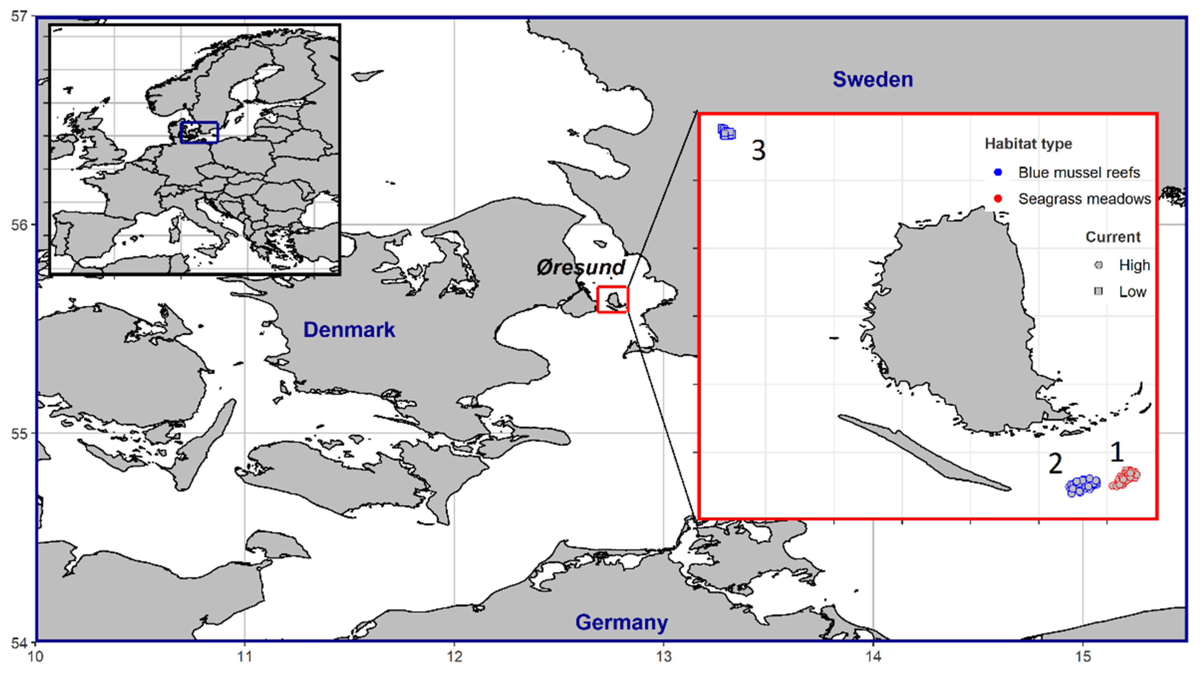
2.1. Study Area

This study was carried out in the Sound (Øresund; ICES subdivision 23) between Denmark and Sweden (Figure 1). The Øresund represents transient waters between the Baltic Sea and Kattegat. Seagrass meadows (Z. marina) occur on sandy sediments at depths ranging between 1–6 m. In total, 162 km2 are covered by seagrass meadows in Øresund [49], whereas blue mussel reefs (M. edulis) cover 46 km2 [50].
Fish abundance and diversity were measured on three field sites near the island of Saltholm in Øresund. Southeast of the island (55°35′12.21″ N; 12°48′04.42″ E), field sites 1 and 2 had high water currents (range: 0.007–1.81 m s−1) (Figure 2a,b). Field site 1 (0.22 km2) provided dense Z. marina meadows, whereas field site 2 (0.28 km2) provided extensive M. edulis reefs.
In contrast, field site 3 (0.17 km2) northwest of the island (55°41′32.63″ N; 12°41′31.68″ E) had low water currents (range: 0.003–0.88 m s−1) (Figure 2a,b) combined with widely developed M. edulis reefs. Comparing additional environmental parameters derived from a numerical operational model, which estimates hourly the hydrographic conditions in the surface water column of Øresund basin (Western Baltic Sea), both sites (site 2 and 3) were characterized by similar water temperature (°C) (Figure 2c,d) and salinity (ppt) (Figure 2e,f). All data were collected during autumn and winter of 2014.

2.2. Fish Assemblages in Z. marina Meadows and M. edulis Reefs

A total of 60 double fyke nets were deployed in Z. marina meadows (field site 1) and M. edulis reefs (field site 2) (high water currents). The lead lengths of fyke nets were 8 m, heights were 0.6 m and mesh sizes were 18 mm. Diameters of the seven sequential hoops were 60, 55, 50, 45, 40, 35 and 35 cm, similar to earlier studies [51]. All fyke nets were deployed identically and with the same orientation to current direction in random positions at field sites 1 and 2 in the afternoon and fished for about 24 h. Deployment and retrieval of the fyke nets followed standard procedures [51,52]. After retrieval, fishes were identified to species or family levels. Catch per unit effort (CPUE) data were derived as the total catch (in numbers) of each taxon for each deployment (i.e., per 24 h). CPUE data were considered proxies of the relative fish abundance following previous studies [53,54,55].

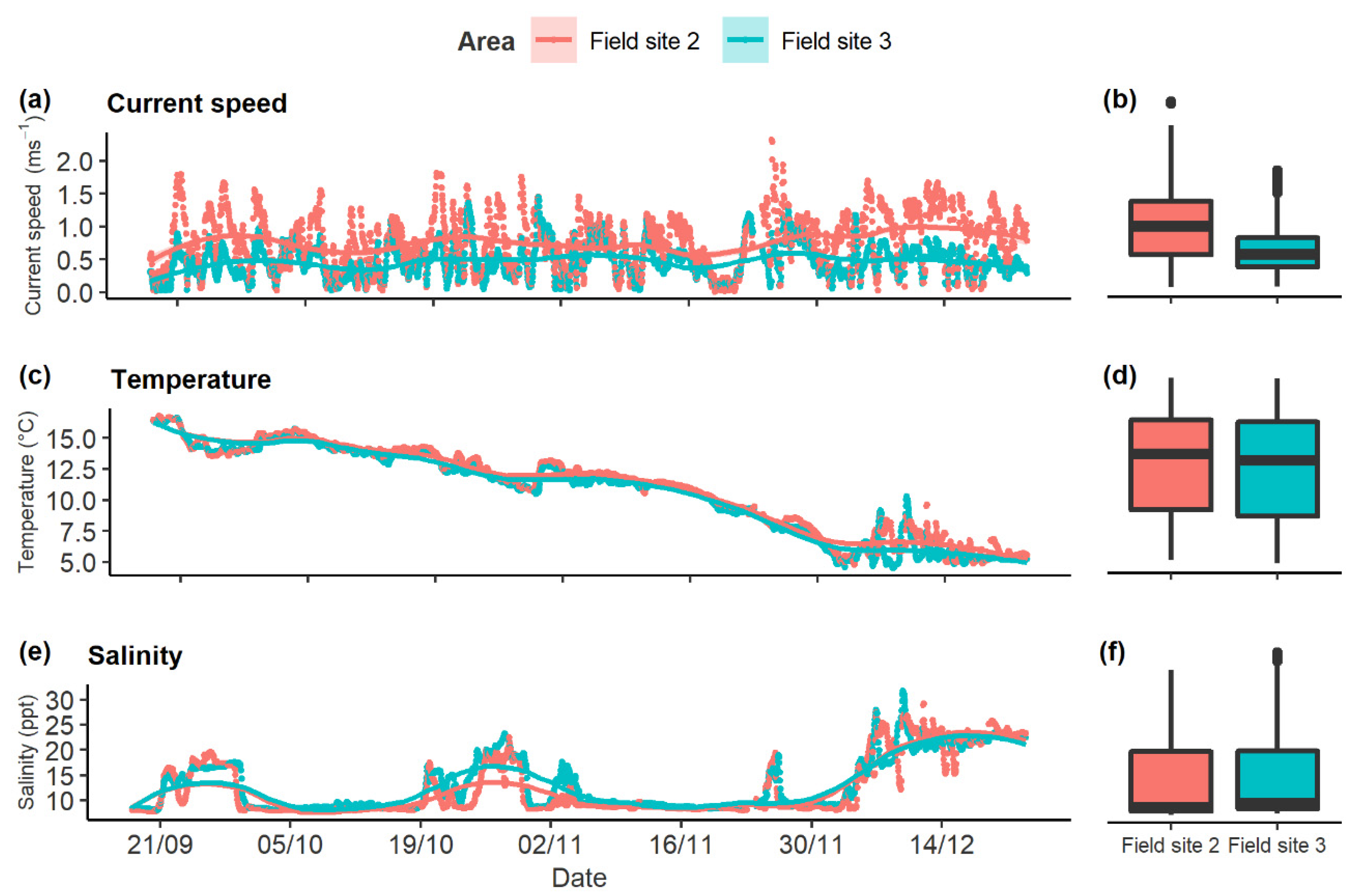
2.3. Fish Assemblages in M. edulis Reefs with High and Low Water Currents

A total of 50 underwater cameras were deployed from 11 September 2014 to 8 December 2014 in contrasting mussel reefs with high currents (HC) and low currents (LC) (i.e., field sites 2 and 3), similar to previous studies using remote underwater video systems to describe fish assemblages in different habitats [56]. Each camera (Hero 3+ Black Edition; GoPro Inc., San Mateo, CA, USA) was mounted with a scheduler (TL-004A Intervalometer; CamDo Solutions Inc, Vancouver, BC, Canada). The scheduler ensured that each camera recorded one 30 s video sequence every hour. Videos were recorded in HDTV resolution (1080 p) with a 30 Hz frame rate and were stored on 32 GB micro-SD cards.
Each camera was mounted for horizontal recording on a vertical pole attached to a concrete tile (40 × 40 × 5 cm). A 10 m line connected the tile to an anchor and surface float. The camera tile was deployed from a boat and lowered to the seafloor with a rope temporarily attached to the tile. After positioning the tile on the seafloor, the rope was retrieved and the anchor line and surface float were deployed.
Similar to previous studies [57,58], video analyses included identifications of fish species or families (when identification to the species level was unreliable) and measurements of the maximum number of each taxon that appeared within the video sequence at one time, know as the MaxN metric. MaxN is a conservative metric of relative abundance and it is used in order to avoid multiple counts of the same individuals appearing in the videos [59,60]. Only daylight recordings were analyzed because no artificial light source was deployed. This approach assumed that recordings between dawn and dusk are sufficient to describe fish assemblages [61,62].

2.4. Statistical Analysis

2.4.1. Statistical Analysis of Fyke Nets Data

Hypothesis 1 stated that fish diversity (i.e., species) and abundance would be higher in seagrass meadows compared to mussel reefs because of higher structural complexities in seagrass meadows [63]. To compare species diversity between Z. marina meadows (field site 1) and M. edulis reefs (field site 2), species richness, Shannon and Pielou’s evenness indices were estimated (R package: vegan, functions: specnumber, diversity [64]). Next, the diversity metrics for each habitat (Z. marina meadow and M. edulis reef) were compared using non-parametric Mann–Whitney tests [65,66] because data were incompatible with a normal distribution, even after transformations.
To contrast fish abundances and composition between Z. marina meadows and M. edulis reefs, a multivariate extension of Generalized Linear Models (GLM), suitable to model abundances of community data (R package: mvabund, function: manyglm [67]) was applied. Due to many zero abundances, leading to overdispersion, a negative binomial regression version of the model was fitted with two levels (mussel reef and seagrass meadow) of habitat as predictor. Multivariate extensions of GLM are considered to increase the statistical power, in comparison to conventional distance-based multivariate analyses, by taking into account the endogenous mean–variance relationship of count type data [68]. To test for significant effects of habitat on fish abundance, univariate analyses of deviance with 999 resampling iterations for each species separately were applied (R package: mvabund, function: anova.manylm [67]). In addition, for the inspection and visualization of the influence of habitat on fish assemblages, a distance-based redundancy analysis (db-RDA) (R package: vegan, function: capscale [64]), using habitat as predictor and Bray–Curtis dissimilarity coefficient, was applied. Finally, a Permutational multivariate analysis of variance (PERMANOVA) [69] (R package: vegan, function: adonis [64]) with Bray–Curtis dissimilarity matrix, was run to test the importance of habitat in explaining the assemblage composition.

2.4.2. Statistical Analysis of Video Cameras’ Data

Hypothesis 2 stated that fish abundance would differ between M. edulis reefs exposed to high (HC) and low (LC) water currents. To address the hypothesis, underwater recordings were analyzed to detect differences between the two habitats. Therefore, differences in the maximum numbers of fish (MaxN) between the two habitats (HC M. edulis reef and LC M. edulis reef) were tested for each species or family separately using a Generalized Linear Mixed Model with negative binomial distribution to avoid pseudoreplication and to account for overdispersion (GLMM, R package: lm4, function: glmer.nb [70]), similar to previous studies [71,72]. The model selection followed [73] and integrated the Akaike Information Criterion (AIC). In addition to the fixed variables of habitat and environmental parameters (salinity, temperature and current), random variables of camera id, hour and month were also included in the model to account for random effects. The species Aphia minuta and sand lances (Ammodytidae) were registered rarely and, thus, were excluded from the analysis. Due to uncertainty in the video identification of gobies (Gobiidae), other than Gobiusculus flavescens and Gobius niger, flatfish (Pleuronectidae) and wrasses (Labridae), other than Ctenolabrus rupestris, they were identified to the family level, while the rest of the fishes were identified to species level.
All statistical analysis and plotting were conducted in R statistical and programming environment (version 3.6.3) [74].

3. Results

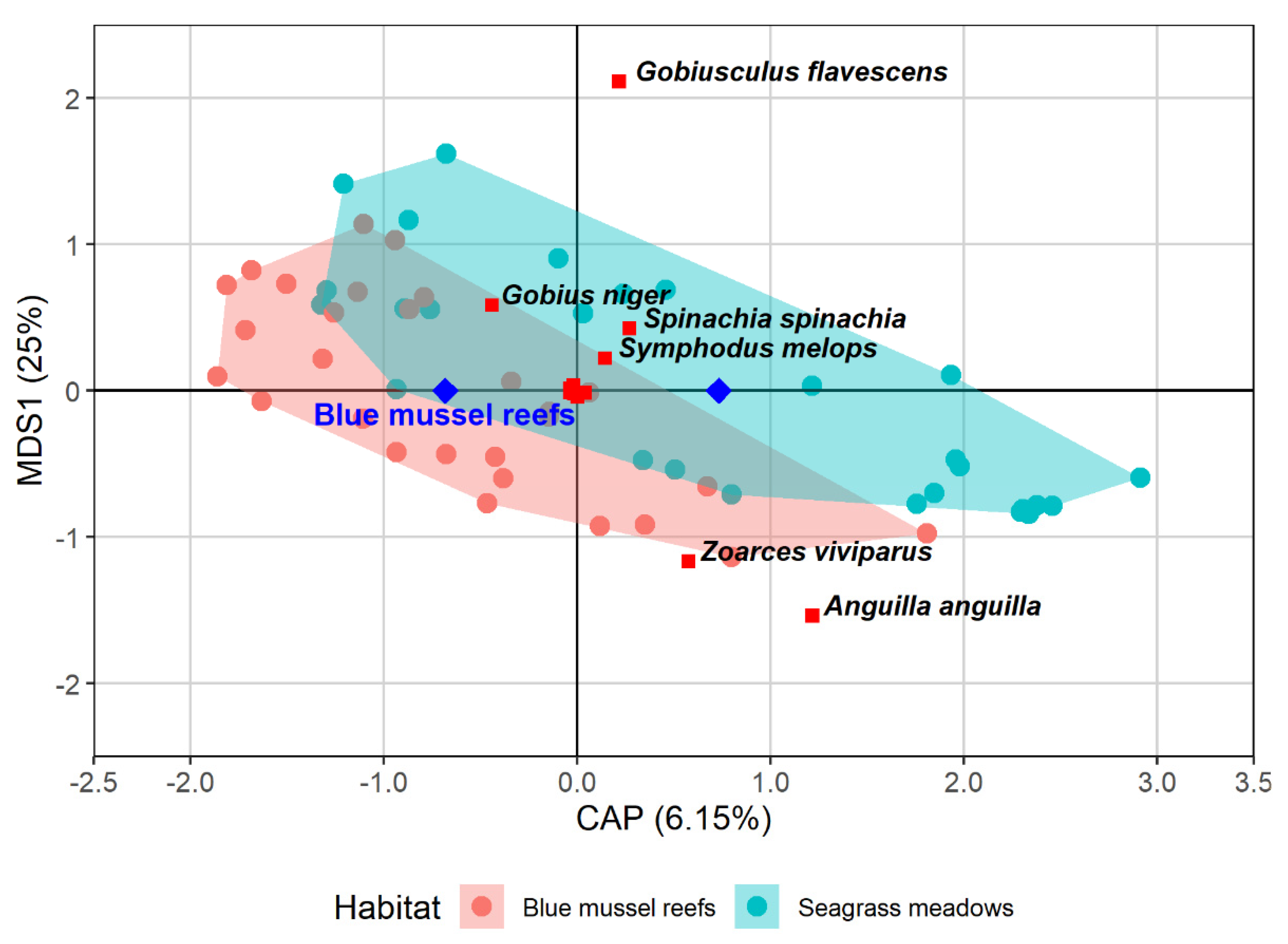
3.1. Using Fyke Nets to Estimate Fish Assemblage in Seagrass Meadows and Mussel Reefs

A total of 380 individual fish, covering 14 different species, were caught by the 60 fyke nets deployed in this study. Eelpout (Zoarces viviparus) was the most abundant species in both surveyed habitats (i.e., seagrass meadow and mussel reef). The eelpout was followed by the two-spotted goby (Gobiusculus flavescens) and the European eel (Anguilla anguilla) in the seagrass meadow and the two-spotted (Gobiusculus flavescens) and black goby (Gobius niger) in the mussel reef habitat. According to the Mann–Whitney test, the habitats provided similar species richness (W = 422, p = 1), the Shannon index (W = 380, p = 0.5) and Pielou’s evenness index (W = 285, p = 0.5) suggested comparative fish species diversities in the two habitats.
The five species broadnosed pipefish (Syngnathus typhle), Atlantic cod (Gadus morhua), corkwing wrasse (Symphodus melops), goldsinny wrasse (Ctenolabrus rupestris) and ninespine stickleback (Pungitius pungitius) were only observed in the mussel habitat, while shorthorn sculpin (Myoxocephalus scorpius) was only found in the seagrass meadows. The total CPUE (i.e., abundance) for all species together was, however, significantly higher in the seagrass meadow (p < 0.001).
The univariate tests comparing the species abundances between the two habitats showed that the CPUE for A. anguilla (p < 0.001) and Z. viviparus (p = 0.02) was significantly higher in the seagrass compared to mussel reef, while the abundance of G. niger was significantly higher (p = 0.01) in the mussel reefs compared to seagrass. All the other species exhibited similar CPUE numbers in both habitats (Table 1).
Based on the distance-based redundancy analysis, the axis of the constrained component (CAP) explained a minor proportion (6.15%) of the variance and the axis of the unconstrained component (MDS1) explained 25% of the residual variation (Figure 3). Even though the proportion of variance explained by habitat in db-RDA was relatively low, the PERMANOVA analysis showed a significant effect of habitat (PERMANOVA, p = 0.003) in distinguishing the assemblages in the two habitats (seagrass meadows and mussel reefs). These findings supported the belief that fish assemblages between seagrass meadows and mussel reefs differ.

3.2. Using Stationary Underwater Cameras to Estimate Fish Assemblage in Two Different Mussel Reef Habitats

For each underwater camera, recordings lasted for 6–7 days (i.e., 300–350 camera days were recorded in total). A total number of 28,535 fish were registered during the video analyses covering the high current (HC) and low current (LC) mussel reefs. The total maximum number of fish was similar (GLMM, p = 0.14) in both habitats. However, the univariate analysis of the maximum number of fish representing each family or species in the two habitats indicated that four species differed significantly. More specifically, G. morhua and C. rupestris exhibited significantly higher abundances in LC mussel reefs, while abundances of G. niger and S. spinachia were higher in HC mussel reefs (Table 2). In addition, flatfish (Pleuronectidae) abundance was higher in LC compared to HC mussel reef, but the statistical test was marginally insignificant (p = 0.0745). Except for habitat, water temperature and salinity demonstrated significant effects on some species. Specifically, temperature had a negative effect on G. morhua abundance (GLMM, p < 0.001), whereas salinity showed a positive effect (GLMM, p = 0.004). Thus, G. morhua abundance appeared to decrease in warmer water and increase at elevated salinities. Concerning the G. flavescens, both water temperature and salinity affected abundance positively (GLMM, p = 0.003 for temperature and p < 0.001 for salinity). Finally, the abundance of C. rupestris was positively affected only by salinity (GLMM, p < 0.001), while the rest of the species and families remained unaffected by environmental variables.

4. Discussion

This study investigated the fish assemblages associated with seagrass meadows and mussel reefs. The study highlights that fish abundance in seagrass meadows is significantly higher compared to mussel reefs. Although the habitats examined supported similar species diversity and richness, the fish assemblages differed slightly in structure. In addition, mussel reef habitats with different water current speeds exhibited similar fish abundances, regardless of the water current regime, revealing minor differences in assemblage composition. However, commercially important species, such as G. morhua and Pleuronectidae, were more abundant in low current mussel reefs. The findings suggest that mussel reef restoration projects should target low current areas if the goal is to support G. morhua and flatfish. Our comparative analysis provides fundamental knowledge for marine habitats and the associated fish assemblages, and plays an important role in the implementation of policies to protect and enhance marine resources, such as coastal fisheries [28,46]. Furthermore, the information combined with species distribution models could be used to define the “essential habitats” for fish life cycles, which should be taken into account in marine spatial planning [75].
Species selectivity of our two sampling methods (fyke nets and underwater cameras) in the same HC mussel bed habitat seemed to differ. More specifically, the two methods presented consistent differences in fish abundance and species composition probably due to different sampling designs, gear selectivity and the sampled area covered by the methods [76,77]. Some species were more effectively targeted by fyke nets (A. anguilla and Z. viviparus), others by the underwater cameras (Labridae and G. morhua), while sampling for other fishes appeared to be unaffected by the gear type (Gobiidae and Pleuronectidae), although the overall fish species spectrum was consistent with previous studies in coastal habitats in the Baltic Sea [17,78,79,80].
The results of this study suggest that species composition may differ between mussel reef and seagrass habitats, highlighting the different ecological value of each habitat. For example, C. rupestris, G. morhua, P. pungitius and S. typhle were only observed at the mussel reefs. The two habitats were, however, characterized by similar species richness (total number of species), e.g., Shannon and Pielou’s evenness indices. These findings are contrary to a previous study [37] that sampled fish with fyke nets in seagrass, oyster and mudflats habitats, and suggested that species composition is more related to location within the estuary than to different habitats. Moreover, in the same study, the authors documented similar fish species richness but marginally higher Shannon diversity in oyster habitats compared to seagrass meadows.
In contrast to the diversity metrics, the overall fish abundance as indexed by CPUE was higher in seagrass meadows, which is in accordance with previous studies [63,81], endorsing that seagrasses support higher fish densities and provide more complex habitats compared to oyster reefs. Additionally, Tomas and Waldbusse [77], comparing seagrass, long-line and on-bottom oyster aquaculture habitats, found higher fish densities in seagrass and long-line oyster habitats compared to on-bottom oyster aquaculture habitats. In contrast, a comparison of fish assemblages in mudflats, oyster reefs and seagrass meadows in North Humboldt Bay, California, showed significantly higher fish CPUE in oyster reefs [44]. To summarize, the majority of previous studies support higher fish abundance in seagrass meadows compared to oyster reefs, a habitat which is similar to mussel reefs as both organisms (oyster and mussel) are bivalves, form biogenic reefs and may offer similar ES.
The relative species composition and fish abundance in both examined habitats (Z. marina meadows and M. edulis reefs) were in agreement with previous studies [4,78,79]. The higher abundance of Z. viviparus in seagrass habitats supports the findings of Thormar et al. [80], reporting that Z. viviparus account for the largest proportion of the fish species in another seagrass area in the western Baltic Sea. Moreover, seagrass meadows exhibited a significantly higher abundance of adult A. anguilla compared to the mussel reefs. In contrast, mussel reefs, as well as medium size gravel habitats, are often favored by juvenile eels [82,83]. A. anguilla is a critically endangered species as stated in the HELCOM Red list [84], as well as in the Danish Red list [85], while Z. viviparous is a near threatened species [84]. A. anguilla is targeted by both commercial and recreational fisheries, although this is highly regulated due to the vulnerable status of the species. On the other hand, Z. viviparous is only occasionally taken for consumption in recreational fisheries. The high abundance of these species in the seagrass habitat and the status of their stocks, as mentioned above, underlines the significant role of seagrass in the ecosystem structure and demonstrates the value of the specific habitats when considering spatial management plans. On the other hand, the only species with significantly higher abundance in mussel reefs compared to seagrass was G. niger, which is a species of “least concern” [86].
The outcomes from the comparison of the two mussel habitats exposed to different current regimes indicated similar total abundance (MaxN) of species in the low and high current habitats, which is consistent with a previous study [41], indicating that the relative fish abundance and fish assemblages of benthic fish species are not strongly structured by current regimes. This finding supports that benthic structures, including biogenic reefs, may act as flow refuges for fish. Other studies have, however, shown increased fish assemblages in high current habitats [39]. In any case, although the outcomes of our research are in accordance with previous studies, conclusions here should be drawn with caution, since the distance between sampling stations was limited, potentially raising issues concerning pseudo-replication.
The distribution of dominant fish species in our study was similar to the distribution of species found in a previous study [17]. Differences in species composition between the mussel reefs with disparate water current regimes may be explained by the absence or presence of the dominant species [87,88]. Specifically, the higher abundance of G. niger in the in HC mussel habitat may be driven by the lower abundance of G. morhua compared to LC mussel reefs, as G. morhua is a major predator of G. niger and the presence of G. morhua alters the behavior of G. niger [89]. Additionally, assemblage structure differences could be explained by the ability of the species to minimize the energy costs in the water current and increase the foraging rates [90]. According to Hamner et al. [91], high current areas could be favored by planktivorous species as the concentration of zooplankton is high in those areas. Thus, the higher abundance of S. spinachia in HC mussel reefs compared to LC could be explained by its slender and elongated body shape, a characteristic which allows for efficient and elevated swimming speeds [92], as well as by its diet preference of small invertebrates including copepods [93].
On the other hand, higher densities of G. morhua and C. rupestris in LC mussel reefs could be attributed to the relatively large body sizes of the fishes with limited opportunity to find shelter against current speeds in the mussel reefs. The negative effect of increasing temperature on G. morhua abundance could be explained by its preference for cooler waters [94]. In addition, the Pleuronectidae family including European flounder (Platichthys flesus), which is a keystone species for the specific area [86], was marginally more abundant in LC mussel reefs than in HC mussel reefs. Therefore, the higher abundances of Pleuronectidae, as well as G. morhua, which is a vulnerable keystone species [84] with high commercial value [95], in the low current mussel reefs compared to the high current mussel reef enforce the importance of protecting low current mussel reefs when spatial management actions are implemented. Thus, it could be most favorable to protect and restore low current mussel reef habitats in management plans to support Pleuronectidae and G. morhua stocks and the economy of various coastal fisheries.
Further research comparing fish assemblages in seagrass and mussel habitats is warranted as it could contribute to a better understanding of habitat use by marine species. In addition, to adequately describe fish assemblages, the selection of the sampling method(s) should be made with caution, especially when management decisions are considered. For example, equipment improvements in cameras, including the use of infrared light (IR), which allows filming in darkness, would allow recordings of the abundance and behavior of nocturnal species. Including sampling of the full diel cycle is important for the evaluation of habitat use, because fish metabolism and behavior may be affected by circadian rhythms [96], potentially resulting in an underestimation of the fish abundances and, subsequently, the importance of the habitat [78,87,94].

5. Conclusions

In this study, we showed that seagrass meadows and mussel reefs in Øresund have a similar fish species diversity and species richness. On the other hand, fish abundance was higher in seagrass meadows as compared to mussel reefs and fish assemblages differed, suggesting that specific habitats may have different ecological and economic value. Concerning the effect of current speeds in mussel reef habitats, fish appeared largely unaffected by the observed variation in current speeds, exhibiting few differences in assemblage structure, although some commercially important species revealed higher abundances in low current mussel reefs. The information should be taken into account by policy makers when management and restoration actions are planned to protect coastal habitats and fisheries [28,45,46,75].

Author Contributions

Conceptualization, C.S. and P.M.; methodology, C.S., G.A.O. and K.T.; software, G.A.O. and K.T.; validation, C.S. and K.T.; formal analysis, G.A.O. and K.T.; investigation, C.S. and P.M.; resources, C.S. and K.T.; data curation, C.S.; writing—original draft preparation, G.A.O.; writing—review and editing, C.S., G.A.O., K.T., J.C.S., J.G.S. and P.M.; visualization, K.T.; supervision, J.C.S.; project administration, C.S. and J.C.S.; funding acquisition, C.S. All authors have read and agreed to the published version of the manuscript.

Funding

This research was funded by the National Institute of Aquatic Resources (DTU Aqua) through a grant from the Danish Rod and Net Fish License Funds (MusFisk; 39 133).

Institutional Review Board Statement

Not applicable.

Informed Consent Statement

Not applicable.

Data Availability Statement

The environmental data presented in the study are available in COPERNICUS database (https://marine.copernicus.eu, accessed on 16 November 2021).

Acknowledgments

The authors thank several DTU Aqua staff members that have been involved in the research. Acknowledgements are also extended to the anonymous reviewers of our manuscript who provided thorough and constructive feedback during the review process. The outcome was an improved paper.

Conflicts of Interest

The authors declare no conflict of interest.

References

  1. Van der Zee, E.M.; Angelini, C.; Govers, L.L.; Christianen, M.; Altieri, A.H.; van der Reijden, K.J.; Silliman, B.R.; van de Koppel, J.; Van der Geest, M.; van Gils, J.A.; et al. How habitat-modifying organisms structure the food web of two coastal ecosystems. Proc. R. Soc. B Biol. Sci. 2016, 283, 20152326. [Google Scholar] [CrossRef] [Green Version]
  2. Peterson, C.H.; Grabowski, J.H.; Powers, S.P. Estimated enhancement of fish production resulting from restoring oyster reef habitat: Quantitative valuation. Mar. Ecol. Prog. Ser. 2003, 264, 249–264. [Google Scholar] [CrossRef] [Green Version]
  3. Orth, R.J.; Carruthers, T.J.B.; Dennison, W.C.; Duarte, C.M.; Fourqurean, J.W.; Heck, K.L.; Hughes, A.R.; Kendrick, G.A.; Kenworthy, W.J.; Olyarnik, S.; et al. A global crisis for seagrass ecosystems. Bioscience 2006, 56, 987–996. [Google Scholar] [CrossRef] [Green Version]
  4. Pihl, L.; Baden, S.; Kautsky, N.; Rönnbäck, P.; Söderqvist, T.; Troell, M.; Wennhage, H. Shift in fish assemblage structure due to loss of seagrass Zostera marina habitats in Sweden. Estuar. Coast. Shelf Sci. 2006, 67, 123–132. [Google Scholar] [CrossRef]
  5. Andersen, J.H.; Laamanen, M.; Aigars, J.; Axe, P.; Blomqvist, M.; Carstensen, J.; Josefson, A.B.; Fleming-Lehtinen, V.; Järvinen, M.; Kaartokallio, H.; et al. HELCOM eutrophication in the Baltic Sea—An integrated thematic assessment of the effects of nutrient enrichment and eutrophication in the Baltic Sea region. In Baltic Sea Environment Proceedings (BSEP) No. 119; Helsinki Commission: Helsinki, Finland, 2009; Volume 115B, p. 148. [Google Scholar]
  6. Eriksson, B.K.; van der Heide, T.; van de Koppel, J.; Piersma, T.; van der Veer, H.W.; Olff, H. Major changes in the ecology of the wadden sea: Human impacts, ecosystem engineering and sediment dynamics. Ecosystems 2010, 13, 752–764. [Google Scholar] [CrossRef] [Green Version]
  7. Beck, M.W.; Heck, K.L.; Able, K.W.; Childers, D.L.; Eggleston, D.B.; Gillanders, B.M.; Halpern, B.; Hays, C.G.; Hoshino, K.; Minello, T.J.; et al. The identification, conservation, and management of estuarine and marine nurseries for fish and invertebrates. Bioscience 2001, 51, 633–641. [Google Scholar] [CrossRef]
  8. Pomeroy, L.R.; D’Elia, C.F.; Schaffner, L.C. Top-down control of phytoplankton by oysters in Chesapeake Bay, USA: Reply to Newell et al. (2007). Mar. Ecol. Prog. Ser. 2007, 341, 299–301. [Google Scholar] [CrossRef]
  9. Grabowski, J.H.; Peterson, C.H. Restoring oyster reefs to recover ecosystem services. In Theoretical Ecology Series; Academic Press: Cambridge, MA, USA, 2007; Volume 4, pp. 281–298. ISBN 9780123738578. [Google Scholar]
  10. Seitz, R.D.; Wennhage, H.; Bergström, U.; Lipcius, R.N.; Ysebaert, T. Ecological value of coastal habitats for commercially and ecologically important species. ICES J. Mar. Sci. J. Cons. 2013. [Google Scholar] [CrossRef] [Green Version]
  11. Kuusemäe, K.; Rasmussen, E.K.; Canal-Vergés, P.; Flindt, M.R. Modelling stressors on the eelgrass recovery process in two Danish estuaries. Ecol. Modell. 2016, 333, 11–42. [Google Scholar] [CrossRef]
  12. Whitfield, A.K. The role of seagrass meadows, mangrove forests, salt marshes and reed beds as nursery areas and food sources for fishes in estuaries. Rev. Fish Biol. Fish. 2016, 1–36. [Google Scholar] [CrossRef]
  13. Lefcheck, J.S.; Hughes, B.B.; Johnson, A.J.; Pfirrmann, B.W.; Rasher, D.B.; Smyth, A.R.; Williams, B.L.; Beck, M.W.; Orth, R.J. Are coastal habitats important nurseries? A meta-analysis. Conserv. Lett. 2019, 12, e12645. [Google Scholar] [CrossRef]
  14. Bromley, C.; McGonigle, C.; Ashton, E.C.; Roberts, D. Restoring degraded European native oyster, Ostrea edulis, habitat: Is there a case for harrowing? Hydrobiologia 2016, 768, 151–165. [Google Scholar] [CrossRef] [Green Version]
  15. Norling, P.; Lindegarth, M.; Lindegarth, S.; Strand, Å. Effects of live and post-mortem shell structures of invasive Pacific oysters and native blue mussels on macrofauna and fish. Mar. Ecol. Prog. Ser. 2015, 518, 123–138. [Google Scholar] [CrossRef] [Green Version]
  16. Gain, I.E.; Brewton, R.A.; Reese Robillard, M.M.; Johnson, K.D.; Smee, D.L.; Stunz, G.W. Macrofauna using intertidal oyster reef varies in relation to position within the estuarine habitat mosaic. Mar. Biol. 2016, 164, 8. [Google Scholar] [CrossRef]
  17. Kristensen, L.D.; Stenberg, C.; Støttrup, J.; Poulsen, L.K.; Christensen, H.T.; Dolmer, P.; Landes, A.; Røjbek, M.; Thorsen, S.W.; Holmer, M.; et al. Establishment of blue mussel beds to enhance fish habitats. Appl. Ecol. Environ. Res. 2015, 13, 783–798. [Google Scholar] [CrossRef]
  18. Norling, P.; Kautsky, N. Patches of the mussel Mytilus sp. are islands of high biodiversity in subtidal sediment habitats in the Baltic Sea. Aquat. Biol. 2008, 4, 75–87. [Google Scholar] [CrossRef] [Green Version]
  19. Koivisto, M.E. Blue Mussel Beds as Biodiversity Hotspots on the Rocky Shores of the Northern Baltic Sea. Ph.D. Thesis, University of Helsinki, Helsinki, Finland, 2011. [Google Scholar]
  20. Reusch, T.; Chapman, A.; Groger, J. Blue mussels Mytilus edulis do not interfere with eelgrass Zostera marina but fertilize shoot growth through biodeposition. Mar. Ecol. Prog. Ser. 1994, 108, 265–282. [Google Scholar] [CrossRef]
  21. Schubert, P.; Hukriede, W.; Karez, R.; Reusch, T. Mapping and modeling eelgrass Zostera marina distribution in the western Baltic Sea. Mar. Ecol. Prog. Ser. 2015, 522, 79–95. [Google Scholar] [CrossRef] [Green Version]
  22. Cullen-Unsworth, L.; Unsworth, R. Seagrass meadows, ecosystem services, and sustainability. Environ. Sci. Policy Sustain. Dev. 2013, 55, 14–28. [Google Scholar] [CrossRef]
  23. Cavanagh, R.D.; Broszeit, S.; Pilling, G.M.; Grant, S.M.; Murphy, E.J.; Austen, M.C. Valuing biodiversity and ecosystem services: A useful way to manage and conserve marine resources? Proc. R. Soc. B Biol. Sci. 2016, 283, 20161635. [Google Scholar] [CrossRef] [Green Version]
  24. Gutiérrez, J.L.; Jones, C.G.; Byers, J.E.; Arkema, K.K.; Berkenbusch, K.; Commito, A.; Duarte, C.M.; Hacker, S.D.; Lambrinos, J.G.; Hendriks, I.E.; et al. Physical ecosystem engineers and the functioning of estuaries and coasts. In Treatise on Estuarine and Coastal Science; Wolanski, E., McLusky, D., Eds.; Academic Press: Waltham, MA, USA, 2012; Volume 7, pp. 53–81. ISBN 9780080878850. [Google Scholar]
  25. Hovel, K.A.; Warneke, A.M.; Virtue-Hilborn, S.P.; Sanchez, A.E. Mesopredator foraging success in eelgrass (Zostera marina L.): Relative effects of epiphytes, shoot density, and prey abundance. J. Exp. Mar. Bio. Ecol. 2016, 474, 142–147. [Google Scholar] [CrossRef]
  26. Bertelli, C.M.; Unsworth, R.K.F. Protecting the hand that feeds us: Seagrass (Zostera marina) serves as commercial juvenile fish habitat. Mar. Pollut. Bull. 2014, 83, 425–429. [Google Scholar] [CrossRef]
  27. Furness, E.; Unsworth, R.K.F. Demersal fish assemblages in NE Atlantic seagrass and Kelp. Diversity 2020, 12, 366. [Google Scholar] [CrossRef]
  28. Nordlund, L.M.; Unsworth, R.K.F.; Gullström, M.; Cullen-Unsworth, L.C. Global significance of seagrass fishery activity. Fish Fish. 2018, 19, 399–412. [Google Scholar] [CrossRef]
  29. Heck, K.L.; Able, K.W.; Fahay, M.P.; Roman, C.T. Fishes and decapod crustaceans of cape cod eelgrass meadows: Species composition, seasonal abundance patterns and comparison with unvegetated substrates. Estuaries 1989, 12, 59. [Google Scholar] [CrossRef]
  30. Unsworth, R.K.F.; Nordlund, L.M.; Cullen-Unsworth, L.C. Seagrass meadows support global fisheries production. Conserv. Lett. 2019, 12, e12566. [Google Scholar] [CrossRef]
  31. Layman, C.A.; Jud, Z.R.; Albrey Arrington, D.; Sabin, D. Using fish behavior to assess habitat quality of a restored oyster reef. Ecol. Restor. 2014, 32, 140–143. [Google Scholar] [CrossRef]
  32. Mark, L.; Harvey, C.J.; Anderson, L.E.; Guerry, A.D.; Ruckelshaus, M.H. The role of eelgrass in marine community interactions and ecosystem services: Results from Ecosystem-Scale Food Web Models. Ecosystems 2013, 16, 237–251. [Google Scholar] [CrossRef]
  33. Fariñas-Franco, J.M.; Roberts, D. Early faunal successional patterns in artificial reefs used for restoration of impacted biogenic habitats. Hydrobiologia 2014, 727, 75–94. [Google Scholar] [CrossRef]
  34. Grabowski, J.H. Habitat complexity disrupts predator-prey interactions but not the trophic cascade on oyster reefs. Ecology 2004, 85, 995–1004. [Google Scholar] [CrossRef] [Green Version]
  35. McDermott, S.; Burdick, D.; Grizzle, R.; Greene, J. Restoring ecological functions and increasing community awareness of an urban tidal pond using blue mussels. Ecol. Restor. 2008, 26, 254–262. [Google Scholar] [CrossRef]
  36. Gratwicke, B.; Speight, M.R. The relationship between fish species richness, abundance and habitat complexity in a range of shallow tropical marine habitats. J. Fish Biol. 2005, 66, 650–667. [Google Scholar] [CrossRef]
  37. Hosack, G.R.; Dumbauld, B.R.; Ruesink, J.L.; Armstrong, D.A. Habitat associations of estuarine species: Comparisons of intertidal mudflat, seagrass (Zostera marina), and oyster (Crassostrea gigas) habitats. Estuaries Coasts 2006, 29, 1150–1160. [Google Scholar] [CrossRef]
  38. Borland, H.P.; Gilby, B.L.; Henderson, C.J.; Leon, J.X.; Schlacher, T.A.; Connolly, R.M.; Pittman, S.J.; Sheaves, M.; Olds, A.D. The influence of seafloor terrain on fish and fisheries: A global synthesis. Fish Fish. 2021, 22, 707–734. [Google Scholar] [CrossRef]
  39. Bey, C.R.; Sullivan, S.M.P. Associations between stream hydrogeomorphology and co-dependent mussel-fish assemblages: Evidence from an Ohio, USA river system. Aquat. Conserv. Mar. Freshw. Ecosyst. 2015, 25, 555–568. [Google Scholar] [CrossRef]
  40. Kerschbaumer, P.; Tritthart, M.; Keckeis, H. Abundance, distribution, and habitat use of fishes in a large river (Danube, Austria): Mobile, horizontal hydroacoustic surveys vs. a standard fishing method. ICES J. Mar. Sci. 2020, 77, 1966–1978. [Google Scholar] [CrossRef]
  41. Eggertsen, L.; Hammar, L.; Gullström, M. Effects of tidal current-induced flow on reef fish behaviour and function on a subtropical rocky reef. Mar. Ecol. Prog. Ser. 2016, 559. [Google Scholar] [CrossRef]
  42. Schmiing, M.; Afonso, P.; Tempera, F. Predictive habitat modelling of reef fishes with contrasting trophic ecologies. Mar. Ecol. Prog. Ser. 2013, 474, 201–216. [Google Scholar] [CrossRef] [Green Version]
  43. Alexander, S.; Aronson, J.; Whaley, O.; Lamb, D. The relationship between ecological restoration and the ecosystem services concept. Ecol. Soc. 2016, 21, 34. [Google Scholar] [CrossRef] [Green Version]
  44. Pinnix, W.D.; Shaw, T.A.; Acker, K.C.; Hetrick, N.J. Fish Communities in Eelgrass, Oyster Culture and Mudflat Habitats of North Humboldt Bay, California, Final Report; USFWS Arcata Fisheries Technical Report TR2005-02; Arcata Fish and Wildlife Office: Arcata, CA, USA, 2005; Volume 95521. [Google Scholar]
  45. Brown, T.; Bergstrom, J.; Loomis, J. Defining, valuing, and providing ecosystem goods and services. Nat. Resour. J. 2007, 47, 329–376. [Google Scholar]
  46. McCormick, H.; Salguero-Gómez, R.; Mills, M.; Davis, K. Using a residency index to estimate the economic value of coastal habitat provisioning services for commercially important fish species. Conserv. Sci. Pract. 2021, 3, e363. [Google Scholar] [CrossRef]
  47. Watermeyer, K.E.; Hutchings, L.; Jarre, A.; Shannon, L.J. Patterns of distribution and spatial indicators of ecosystem change based on key species in the southern Benguela. PLoS ONE 2016, 11, e0158734. [Google Scholar] [CrossRef] [Green Version]
  48. Long, R.D.; Charles, A.; Stephenson, R.L. Key principles of marine ecosystem-based management. Mar. Policy 2015, 57, 53–60. [Google Scholar] [CrossRef]
  49. Boström, C.; Baden, S.; Bockelmann, A.C.; Dromph, K.; Fredriksen, S.; Gustafsson, C.; Krause-Jensen, D.; Möller, T.; Nielsen, S.L.; Olesen, B.; et al. Distribution, structure and function of Nordic eelgrass (Zostera marina) ecosystems: Implications for coastal management and conservation. Aquat. Conserv. Mar. Freshw. Ecosyst. 2014, 24, 410–434. [Google Scholar] [CrossRef] [PubMed] [Green Version]
  50. Jensen, A.; Lyngby, J.E. Environmental management and monitoring at the Øresund fixed link. Terra Aqua 1999, 74, 10–20. [Google Scholar]
  51. Stenberg, C.; Støttrup, J.; Dahl, K.; Lundsteen, S.; Göke, C.; Andersen, O.N. Ecological Benefits from Restoring a Marine Cavernous Boulder Reef in Kattegat, Denmark; National Institute of Aquatic Resources, Danmarks Tekniske Universitet: Lyngby, Denmark, 2015. [Google Scholar]
  52. Kleiven, A.R.; Fernandez-Chacon, A.; Nordahl, J.-H.; Moland, E.; Espeland, S.H.; Knutsen, H.; Olsen, E.M. Harvest pressure on coastal Atlantic cod (Gadus morhua) from recreational fishing relative to commercial fishing assessed from tag-recovery data. PLoS ONE 2016, 11, e0149595. [Google Scholar]
  53. Kerwath, S.E.; Winker, H.; Götz, A.; Attwood, C.G. Marine protected area improves yield without disadvantaging fishers. Nat. Commun. 2013, 4, 2347. [Google Scholar] [CrossRef] [PubMed]
  54. Reubens, J.T.; Braeckman, U.; Vanaverbeke, J.; Van Colen, C.; Degraer, S.; Vincx, M. Aggregation at windmill artificial reefs: CPUE of Atlantic cod (Gadus morhua) and pouting (Trisopterus luscus) at different habitats in the Belgian part of the North Sea. Fish. Res. 2013, 139, 28–34. [Google Scholar] [CrossRef]
  55. Adams, G.D.; Flores, D.; Flores, O.G.; Aarestrup, K.; Svendsen, J.C. Spatial ecology of blue shark and shortfin mako in southern Peru: Local abundance, habitat preferences and implications for conservation. Endanger. Species Res. 2016, 31, 19–32. [Google Scholar] [CrossRef] [Green Version]
  56. Rhodes, N.; Wilms, T.; Baktoft, H.; Ramm, G.; Bertelsen, J.L.; Flávio, H.; Støttrup, J.G.; Kruse, B.M.; Svendsen, J.C. Comparing methodologies in marine habitat monitoring research: An assessment of species-habitat relationships as revealed by baited and unbaited remote underwater video systems. J. Exp. Mar. Biol. Ecol. 2020, 526, 151315. [Google Scholar] [CrossRef]
  57. Cappo, M.; Speare, P.; De’Ath, G. Comparison of baited remote underwater video stations (BRUVS) and prawn (shrimp) trawls for assessments of fish biodiversity in inter-reefal areas of the Great Barrier Reef Marine Park. J. Exp. Mar. Biol. Ecol. 2004, 302, 123–152. [Google Scholar] [CrossRef]
  58. Becker, A.; Taylor, M.D.; Lowry, M.B. Monitoring of reef associated and pelagic fish communities on Australia’s first purpose built offshore artificial reef. ICES J. Mar. Sci. 2016, 74, 277–285. [Google Scholar] [CrossRef]
  59. Ellis, D.; DeMartini, E. Evaluation of a video camera technique for indexing abundances of juvenile pink snapper, Pristipomoides filamentosus, and other Hawaiian insular shelf fishes. Fish. Bull. 1995, 93, 67–77. [Google Scholar]
  60. Priede, I.G.; Merrett, N.R. Estimation of abundance of abyssal demersal fishes; a comparison of data from trawls and baited cameras. J. Fish Biol. 1996, 49, 207–216. [Google Scholar] [CrossRef]
  61. Sogard, S.M.; Powell, G.V.N.; Holmquist, J.G. Epibenthic fish communities on Florida Bay banks: Relations with physical parameters and seagrass cover. Mar. Ecol. Prog. Ser. 1987, 40, 25–39. [Google Scholar] [CrossRef]
  62. Aller, E.A.; Gullström, M.; Eveleens Maarse, F.K.J.; Gren, M.; Nordlund, L.M.; Jiddawi, N.; Eklöf, J.S. Single and joint effects of regional- and local-scale variables on tropical seagrass fish assemblages. Mar. Biol. 2014, 161, 2395–2405. [Google Scholar] [CrossRef]
  63. Minello, T.J.; Able, K.W.; Weinstein, M.P. Salt marshes as nurseries for nekton: Testing hypotheses on density, growth and survival through meta-analysis. Mar. Ecol. Prog. Ser. 2003, 246, 39–59. [Google Scholar] [CrossRef]
  64. Oksanen, A.J.; Blanchet, F.G.; Friendly, M.; Kindt, R.; Legendre, P.; Mcglinn, D.; Minchin, P.R.; O’Hara, R.B.; Simpson, G.L.; Solymos, P.; et al. Vegan Community Ecology Package, R Package Version 2.5-7; 28 November 2020. Available online: https://mran.microsoft.com/package/vegan (accessed on 14 November 2021).
  65. Audebert, C.; Even, G.; Cian, A.; Loywick, A.; Merlin, S.; Viscogliosi, E.; Chabé, M. Colonization with the enteric protozoa Blastocystis is associated with increased diversity of human gut bacterial microbiota. Sci. Rep. 2016, 6, 25255. [Google Scholar] [CrossRef]
  66. Matteodo, M.; Ammann, K.; Verrecchia, E.P.; Vittoz, P. Snowbeds are more affected than other subalpine-alpine plant communities by climate change in the Swiss Alps. Ecol. Evol. 2016, 6, 6969–6982. [Google Scholar] [CrossRef]
  67. Wang, Y.; Naumann, U.; Wright, S.T.; Warton, D.I. mvabund–an R package for model-based analysis of multivariate abundance data. Methods Ecol. Evol. 2012, 3, 471–474. [Google Scholar] [CrossRef]
  68. Warton, D.I.; Wright, S.T.; Wang, Y. Distance-based multivariate analyses confound location and dispersion effects. Methods Ecol. Evol. 2012, 3, 89–101. [Google Scholar] [CrossRef]
  69. Anderson, M.J. A new method for non-parametric multivariate analysis of variance. Austral Ecol. 2001, 26, 32–46. [Google Scholar] [CrossRef]
  70. Bates, D.; Mächler, M.; Bolker, B.; Walker, S. Fitting linear mixed-effects models using lme4. J. Stat. Softw. 2015, 67, 1–48. [Google Scholar] [CrossRef]
  71. Sequeira, A.M.M.; Mellin, C.; Lozano-Montes, H.M.; Meeuwig, J.J.; Vanderklift, M.A.; Haywood, M.D.E.; Babcock, R.C.; Caley, M.J. Challenges of transferring models of fish abundance between coral reefs. PeerJ 2018, 6, e4566. [Google Scholar] [CrossRef] [PubMed] [Green Version]
  72. Wood, C.L.; Summerside, M.; Johnson, P.T.J. An effective method for ecosystem-scale manipulation of bird abundance and species richness. Ecol. Evol. 2019, 9, 9748–9758. [Google Scholar] [CrossRef] [Green Version]
  73. Christ, A. Mixed effects models and extensions in Ecology with R. J. Stat. Softw. 2009, 32, 1–3. [Google Scholar] [CrossRef] [Green Version]
  74. R Core Team. R: A Language and Environment for Statistical Computing; R Core Team: Vienna, Austria, 2020. [Google Scholar]
  75. Katara, I.; Peden, W.J.; Bannister, H.; Ribeiro, J.; Fronkova, L.; Scougal, C.; Martinez, R.; Downie, A.; Sweeting, C.J. Conservation hotspots for fish habitats: A case study from English and Welsh waters. Reg. Stud. Mar. Sci. 2021, 44, 101745. [Google Scholar] [CrossRef]
  76. Bergström, L.; Karlsson, M.; Pihl, L. Comparison of Gill Nets and Fyke Nets for the Status Assessment of Coastal fish Communities; WATERS Report no. 2013:7; Havsmiljöinstitutet: Gothenburg, Sweden, 2013; Deliverable 3.4-2. [Google Scholar]
  77. KA, M.; Tomas, F.; Waldbusser, G. On the edge: Assessing fish habitat use across the boundary between Pacific oyster aquaculture and eelgrass in Willapa Bay, Washington, USA. Aquac. Environ. Interact. 2020, 12, 541–557. [Google Scholar]
  78. Bobsien, I.C.; Brendelberger, H. Comparison of an enclosure drop trap and a visual diving census technique to estimate fish populations in eelgrass habitats. Limnol. Oceanogr. Methods 2006, 4, 130–141. [Google Scholar] [CrossRef]
  79. Bergström, L.; Sundqvist, F.; Bergström, U. Effects of an offshore wind farm on temporal and spatial patterns in the demersal fish community. Mar. Ecol. Prog. Ser. 2013, 485, 199–210. [Google Scholar] [CrossRef] [Green Version]
  80. Thormar, J.; Hasler-Sheetal, H.; Baden, S.; Boström, C.; Clausen, K.K.; Krause-Jensen, D.; Olesen, B.; Rasmussen, J.R.; Svensson, C.J.; Holmer, M. Eelgrass (Zostera marina) food web structure in different environmental settings. PLoS ONE 2016, 11, e0146479. [Google Scholar] [CrossRef] [PubMed] [Green Version]
  81. Kelly, J.R.; Proctor, H.; Volpe, J.P. Intertidal community structure differs significantly between substrates dominated by native eelgrass (Zostera marina L.) and adjacent to the introduced oyster Crassostrea gigas (Thunberg) in British Columbia, Canada. Hydrobiologia 2008, 596, 57–66. [Google Scholar] [CrossRef]
  82. Schwartzbach, A.; Munk, P.; Sparholt, H.; Christoffersen, M. Marine mussel beds as attractive habitats for juvenile European eel (Anguilla anguilla); A study of bottom habitat and cavity size preferences. Estuar. Coast. Shelf Sci. 2020, 246, 107042. [Google Scholar] [CrossRef]
  83. Christoffersen, M.; Svendsen, J.C.; Kuhn, J.A.; Nielsen, A.; Martjanova, A.; Støttrup, J.G. Benthic habitat selection in juvenile European eel Anguilla anguilla: Implications for coastal habitat management and restoration. J. Fish Biol. 2018, 93, 996–999. [Google Scholar] [CrossRef] [PubMed] [Green Version]
  84. Helsinki Commission. HELCOM Red List of Baltic Sea Species in Danger of Becoming Extinct; Baltic Sea Environmental Proceedings No 140; Helsinki Commission: Helsinki, Finland, 2013; Volume 140, ISSN 0357-2994. [Google Scholar]
  85. Carl, H.; Møller, P.R. Fisk. In Moeslund, J.E. m.fl. (red.): Den Danske Rødliste 2019; Nationalt Center for Miljø og Energi: Roskilde, Denmark, 2019. [Google Scholar]
  86. Helsinki Commission. HELCOM Red List of Threatened and Declining Species of Lampreys and Fishes of the Baltic Sea; Baltic Sea Environmental Proceedings No 109; Helsinki Commission: Helsinki, Finland, 2006; ISSN 0357-294. [Google Scholar]
  87. Thedinga, J.F.; Johnson, S.W.; Neff, A.D. Diel differences in fish assemblages in nearshore eelgrass and kelp habitats in Prince William Sound, Alaska. Environ. Biol. Fishes 2011, 90, 61–70. [Google Scholar] [CrossRef]
  88. Pessanha, A.L.M.; Araújo, F.G.; De Azevedo, M.C.C.; Gomes, I.D. Diel and seasonal changes in the distribution of fish on a southeast Brazil sandy beach. Mar. Biol. 2003, 143, 1047–1055. [Google Scholar] [CrossRef]
  89. Magnhagen, C. Reproduction under predation risk in the sand goby, Pomatoschistus minutes, and the black goby, Gobius niger: The effect of age and longevity. Behav. Ecol. Sociobiol. 1990, 26, 331–335. [Google Scholar] [CrossRef]
  90. Fausch, K.D. Profitable stream positions for salmonids: Relating specific growth rate to net energy gain. Can. J. Zool. 1984, 62, 441–451. [Google Scholar] [CrossRef]
  91. Hamner, W.M.; Jones, M.S.; Carleton, J.H.; Hauri, I.R.; Williams, D.M. Zooplankton, planktivorous fish, and water currents on a windward reef face: Great Barrier Reef, Australia. Bull. Mar. Sci. 1988, 42, 459–479. [Google Scholar]
  92. Baktoft, H.; Jacobsen, L.; Skov, C.; Koed, A.; Jepsen, N.; Berg, S.; Boel, M.; Aarestrup, K.; Svendsen, J.C. Phenotypic variation in metabolism and morphology correlating with animal swimming activity in the wild: Relevance for the OCLTT (oxygen- and capacity-limitation of thermal tolerance), allocation and performance models. Conserv. Physiol. 2016, 4, cov055. [Google Scholar] [CrossRef] [Green Version]
  93. Kullander, S.O.; Nyman, L.; Jilg, K.; Delling, B. Nationalnyckeln till Sveriges flora och fauna. Strålfeniga fiskar. Actinopterygii; SLU Artdatabanken: Uppsala, Sweden, 2012; ISBN 978-91-88506-80-1. [Google Scholar]
  94. Carla, F.; Olsen, E.; Knutsen, H.; Albretsen, J.; Moland, E. Temperature-associated habitat selection in a cold-water marine fish. J. Anim. Ecol. 2015, 85, 628–637. [Google Scholar] [CrossRef] [Green Version]
  95. International Council for the Exploration of the Sea. ICES Report of the ICES Advisory Committee 2012; ICES Advise 2012; International Council for the Exploration of the Sea: Copenhagen, Denmark, 2012; p. 389. [Google Scholar]
  96. Svendsen, J.C.; Genz, J.; Anderson, W.G.; Stol, J.A.; Watkinson, D.A.; Enders, E.C. Evidence of circadian rhythm, oxygen regulation capacity, metabolic repeatability and positive correlations between forced and spontaneous maximal metabolic rates in lake sturgeon Acipenser fulvescens. PLoS ONE 2014, 9, e94693. [Google Scholar] [CrossRef] [PubMed] [Green Version]
Figure 1. Map of the sampling area and sites. The red color dots indicate the seagrass meadows (field site 1), while the blue color dots indicate the mussel reefs. For the mussel reefs, circles refer to high water currents (field site 2) and squares refer to low water currents (field site 3).
Water 13 03268 g001
Figure 2. Environmental variables across the study period (September to December 2014) in the mussel reef areas with high currents (HC) (red color) (field site 2) and with low currents (LC) (green color) (field site 3): (a) water current speeds (m s−1); (c), water temperature (°C); (e) water salinity (ppt); (b,d,f) boxplots representing the mean values of the environmental parameters (a,c,e, respectively) for each site with 95% confidence intervals. The environmental data are derived from a numerical operational model, which estimates the hydrographic conditions in the Øresund basin (Western Baltic Sea). The database Baltic Sea Analyses Forecast was used, accessible via COPERNICUS (https://marine.copernicus.eu/, accessed on 16 November 2021).
Water 13 03268 g002
Figure 3. Distance-based redundancy analysis (db-RDA) of the abundances of fish families and species with habitat (i.e., seagrass meadow and mussel reef) as predictor. The green convex hull and point (circles) refer to the seagrass meadows (high current; field site 1), while the red convex hull and point (circles) refer to the mussel reefs (high current; field site 2) in the Western Baltic Sea (Øresund). Red square represents the species (species names are shown when the distance from the center of the axes is >0.1).
Water 13 03268 g003
Table 1. Comparison of fish species abundances estimated using catch per unit effort (CPUE) data from seagrass meadows and mussel reefs in the Øresund between Denmark and Sweden. The p values were derived from the univariate analyses of deviance with 999 resampling iterations, comparing the number of each species separately in each habitat. The bold cells indicate the statistically significant differences and the asterisks show the level of significance, where *** p < 0.001 and * p < 0.05.
FamilyFish Species Latin NameCommon NameCPUE
Mussel
CPUE
Seagrass
pDev
AnguillidaeAnguilla anguillaEuropean eel0.32.429<0.001 ***12.15
LabridaeCtenolabrus rupestrisGoldsinny wrasse0.06700.182.64
GadidaeGadus morhuaAtlantic cod0.06700.142.64
GobiidaeGobius nigerBlack goby1.20.4290.01 *6.45
GobiidaeGobiusculus flavescensTwo-spotted goby1.3331.7140.610.28
CottidaeMyoxocephalus scorpiusShorthorn sculpin00.0710.132.91
PleuronectidaePlatichthys flesusEuropean flounder0.0670.0360.680.27
PleuronectidaePleuronectes platessaEuropean plaice0.0330.0360.860
GasterosteidaePungitius pungitiusNinespine stickleback0.03300.471.32
GasterosteidaeSpinachia spinachiaSea stickleback0.1330.6070.112.96
LabridaeSymphodus melopsCorkwing wrasse0.0330.2860.064.1
SyngnathidaeSyngnathus typhleBroadnosed pipefish0.03300.441.32
CottidaeTaurulus bubalisLongspined bullhead0.0670.0360.650.27
ZoarcidaeZoarces viviparusEelpout1.62.6070.02 *5.79
Table 2. Comparison of mean fish abundances (in terms of MaxN) with associated confidence intervals (CI), recorded by underwater cameras in mussel reefs with high and low water currents in Øresund. The p values were derived from tests using a GLMM model with negative binomial distribution comparing the maximum number of fish between mussel reefs with high and low current speeds. The asterisks show the level of significance, where *** p < 0.001 and * p < 0.05.
FamilyFish SpeciesCommon NameMean
Abundance in High Current Mussel Reef
CI for High CurrentMean
Abundance in Low
Current Mussel Reef
CI for Low Currentp
GadidaeGadus morhuaAtlantic cod0.00000.6210.446–0.864<0.001 ***
GasterosteidaeGasterosteus
aculeatus
Three-spined stickleback0.0000–0.0380.0000–0.0040.485
GobiidaeGobius nigerBlack goby0.3790.154–0.9310.0230.006–0.087<0.001 ***
GobiidaeGobiusculus
flavescens
Two-spotted goby10.1353.112–33.00221.2216.107–73.7360.3876
Gobiidae Other gobies0.0840.012–0.6090.2830.022–3.6070.2511
LabridaeCtenolabrus rupestrisGoldsinny wrasse0.0170.003–0.0860.5150.157–1.694<0.001 ***
Labridae Other wrasses0.0000–0.0060.0000–0.0050.7568
Pleuronectidae Flatfish0.0100.001–0.1660.0410.002–0.9450.0745
GasterosteidaeSpinachia spinachiaSea stickleback0.0580.022–0.1490.0060.001–0.0480.043 *
Publisher’s Note: MDPI stays neutral with regard to jurisdictional claims in published maps and institutional affiliations.

