Modeling Local Scour around a Cylindrical Pier with Circular Collar with Tilt Angles (Counterclockwise around the Direction of the Channel Cross-Section) in Clear-Water

Abstract

This research explores how a circular collar with a tilt angle (counterclockwise around the direction of the channel cross-section) could affect the local scour depth around a single cylindrical pier in clear-water based on Large Eddy Simulation (LES) in six cases. The results show that a horizontal circular collar is the best for reducing the local scour depth. With the increases of the tilt angle, the effect on reducing the local scour depth decreases gradually and is even counterproductive at the scour equilibrium. At the early stage of scouring, cases with circular collars show obvious scouring depth reductions. The smaller the tilt angle is, the better and longer-lasting the protection that the circular collar can provide. When the tilt angle is smaller than 5°, the location of the maximum local scouring is around 90–115° (the angle is measured clockwise from the flow direction) on both sides of the pier. When the tilt angle is greater than 5°, the depth of local scouring in the range around −115° to 115° is close to the maximum local scouring depth. Significantly larger areas reach the maximum scouring depth when the tilt angle increases. Compared to Case 1 (the pier without a circular collar), in the cases with a circular collar, the topographies downwards the pier in 1.0D (D is the diameter of the bridge pier) are changed to siltation from scouring. The topography downwards the pier changes from scouring to siltation with the increase of the tilt angle, and the shape of siltation changes from a long-narrow rectangle to an equilateral triangle. This study may provide valuable insights into the protection of the local scour of the pier.

1. Introduction

Local scour is a natural phenomenon and usually occurs near obstructions such as piers and abutments. It is caused by horseshoe vortices forming near the base of the obstructions and the wake vortices forming in the separation zone. These vortices remove the sediment near the obstructions and reduce stability [1,2]. Scour is the main cause of the failures of highway bridges all over the world, such as in China, the USA, the UK, New Zealand, and so on [3]. The USA and China are two of the countries that have suffered serious losses in bridge failures. In the United States, 58% of 1502 major bridge failures were caused by scouring near piers from 1966 to 2005 [4]. In China, more than 30% of 106 bridge failures were caused by scouring near piers from 2000 to 2014 [5]. Therefore, the mechanism of the local scour and the reduction measures for local scour have been such an important interest to researchers all over the world. The results showed that the dominant feature of the flow near a pier is a large-scale eddy structure or the system of vortices developed by the pier and these vortex systems are the basic mechanism of local scour. Melville [6] studied the mechanism of local scour at a circular cylinder by experiments. The results showed that the scour is caused by the high local shear stresses generated by the acceleration of flow around the cylinder, and the subsequent development of the scour hole is due to the establishment of a strong downflow in front of the cylinder. The horseshoe vortex is small and weak at the beginning with a roughly circular cross-section, but the size and strength increase with the formation, expansion, and downwards motion in the scour hole. The circulation increases throughout the scour process. Chiew and Melville [7] studied the local scour around cylindrical bridge piers in uniform, cohesionless sediment by experiment. The empirical functions of the equilibrium scour depth with approach velocity and the sediment size were obtained. Melville and Sutherland [8] studied the method for the estimation of equilibrium depths of local scour at bridge piers by laboratory experiments. Melville [9] studied the relationship between the local scour depth at a bridge pier and the flood, the bed sediment characteristics, and the geometry of the bridge pier.

Based on the results of the mechanism of local scour around the pier, research was carried out to find effective ways to reduce the maximum scour depth. Deng and Cia [10] studied the local scour depth of the pier with the protection of a collar with a rounded shape and found that the flow was divided into two parts by the collar, one above the collar and the other one below the collar. The size and location of the collar are the two key factors that affect the local scour depth. Negm et al. [11] studied the local scour depth of a cylindrical pier with different shapes and widths of the collar. The results showed that the scour depth is reduced with the increase of the width of the collar. Ardeshiri et al. [12] studied the local scour depth of a cylindrical pier with a collar of three different shapes, and the results show that the lozenge collar is more efficient. Jahangirzadeh et al. [13] studied the local scour depth of a cylindrical pier with rectangular collar and circular collar by experiment and simulation, and the results indicated that the rectangular collar is more effective. Chen et al. [14] studied the local scour depth of a cylindrical pier with a hooked collar at two different locations, and the results indicated that the collar at the bed level is more effective.

With the development of computer science, software based on Computational Fluid Dynamics (CFD) is widely adopted, which can not only help visualize the scouring process but can also provide accurate and reliable results with comparison to the results by experiment [15,16,17,18,19,20,21,22,23,24,25,26,27,28]. At present, the RANS (Reynolds Averaged Navier-Stokes Simulation) and the LES (Large Eddy Simulation) are two main numerical modes of 3D turbulence simulation. The basic idea of RANS is to solve the time-averaged Navier-Stokes equation for all scales of motion in a turbulent flow. So, it can produce time-averaged velocity and sediment concentration but could not show the effects of the unsteadiness and turbulence anisotropy on sediment transports. LES is built based on different roles of flows of different scales in transport and dissipation. In turbulent flow, the large-scale flow dominates the momentum and energy transport, while the dissipation of turbulent kinetic energy mainly occurs in small-scale flow. A flow is divided into large eddies and sub-grid eddies in LES. The large-scale ones are solved directly by using the Navier-Stokes equation, and the small-scale ones are simulated by using the Sub-Grid Stress model, which means only small-scale simulation variables are simulated in LES [29,30,31,32,33,34,35]. Therefore, LES fits more in complex turbulent structures, and the results are closer to the actual situation. So, LES is wildly used in the field of CFD [36,37,38,39,40,41,42].

In the field of open-channel flow and sediment transport, van Balen et al. [43] studied the flow over topography in a curved open-channel by Large Eddy Simulation. Bai et al. [44] studied the transport and settling of suspended sediments affected by the aspect ratio of the channel. The results show that the channel aspect ratio has a large influence on the distribution of suspended sediments within the cross-section, and the effect on the cross-sectional averaged deposition is negligibly small. Chou and Fringer [45] studied the sediment suspension using Large Eddy Simulation with a dynamic mixed model. Khosronejad et al. [46,47] studied the rigid lid and level set methods for LES of open-channel flow. McCoy et al. [48,49] used LES to study the flow hydrodynamics in a groin field and found that most of the fluid leaves the embayment via the top layer of the channel-embayment interface (upstream half) and enters the embayment at levels situated around the mid-depth. Constantinescu et al. [50] studied the direct link between the mechanism of mass exchange and the dynamics of coherent structures using LES in a shallow channel flow with a series of groins. Brevis et al. [51] find that the effects of obstacles on the main channel are up to the length of the obstacle in the span-wise direction; the spacing between obstacles does not seem to have considerable influence on the outer flow. Kirkil et al. [52] studied the coherent structures in the flow field around a circular cylinder with a scour hole. Koken and Constantinescu [53,54] studied the flow and scour mechanisms around isolated spur dikes in a shallow open channel in conditions corresponding to the initiation of the erosion and deposition process and the final stages of the erosion and deposition process. The above research results have important guidance and reference for both theoretical and practical engineering.

Due to an easier way to build, the circular collar designed horizontally on the surface of the riverbed has been widely used in actuality. However, it is difficult to build an absolute horizontal collar in actuality, and that will reduce its protective effect. On the other hand, when an absolute horizontal circular collar cannot be guaranteed, what tilt angles are acceptable? What are the characteristics and effects of the circular collar with tilt angles on local scour depth reduction? All the above aspects are worthy of attention and exploration. Research results of the influences of tilt angles of the collar on the local scouring depth around the cylindrical pier have been rarely reported. This study will focus on the local scour around a cylindrical pier with a circular collar. The circular collars in different cases are rotated counterclockwise in different angles around the direction of the channel cross-section in clear-water using the Large Eddy Simulation (LES) model, which has proven to be competent for the simulation of local scour. This study mainly includes the following two parts:

(1)

the numerical modeling and setup, including the introduction of LES, the verification of the method used in this study, the model and parameters studied in this paper;

(2)

the results and discussion, including the characteristics of the local scour depth and the topography around the pier in each case and the characteristics and mechanism of the effects of the circular collar with tilt angles on local scour depth around a single cylindrical pier.

2. Numerical Modeling and Setup

Flow-3D is one of the Computational Fluid Dynamics (CFD) codes, which was widely used to solve the problems of multi-physics flow because of its simple, faster, and more powerful meshing capability. The Volume of Fluid (VOF) is a typical model of Flow-3D, which was used to solve the nonlinear Navier-Stokes equation, and to track the free surface of flow in a broad range of fields, such as in an open channel. Therefore, Flow-3D was used in this study.

2.1. Governing Equations of LES

Large Eddy Simulation (LES) is a numerical technique for integrating spatially filtered equations of the motion that describes the high-Reynolds number time-evolving, three-dimensional turbulence. The spatial filtering cuts off the high frequency or small-scale part of the turbulence spectrum. The governing equations employed for LES are obtained by filtering the time-dependent Navier-Stokes equations. The filtering process effectively filters out the eddies whose scales are smaller than the filter width or grid spacing used in the computations. The equations of large eddies are shown as follows:

$$\frac{\partial \mathsf{\rho }}{\partial \mathrm{t}}+\frac{\partial \left(\mathsf{\rho }\overline{{\mathrm{u}}_{\mathrm{i}}}\right)}{\partial {\mathrm{x}}_{\mathrm{i}}}=0$$

(1)

$$\mathsf{\rho }\frac{\partial \left(\overline{{\mathrm{u}}_{\mathrm{i}}}\right)}{\partial \mathrm{t}}+\mathsf{\rho }\frac{\partial \left(\overline{{\mathrm{u}}_{\mathrm{i}}}\overline{{\mathrm{u}}_{\mathrm{j}}}\right)}{\partial {\mathrm{x}}_{\mathrm{j}}}=-\frac{\partial \overline{\mathrm{p}}}{\partial {\mathrm{x}}_{\mathrm{i}}}+\mathsf{\mu }\frac{{\partial }^2\overline{{\mathrm{u}}_{\mathrm{i}}}}{\partial {\mathrm{x}}_{\mathrm{j}}^2}-\mathsf{\rho }\frac{\partial {\mathsf{\tau }}_{\mathrm{ij}}}{\partial {\mathrm{x}}_{\mathrm{j}}}$$

(2)

$${\mathsf{\tau }}_{\mathrm{ij}}=\overline{{\mathrm{u}}_{\mathrm{i}}{\mathrm{u}}_{\mathrm{j}}}-\overline{{\mathrm{u}}_{\mathrm{i}}}\overline{{\mathrm{u}}_{\mathrm{j}}}$$

(3)

where x_i (i = 1, 2, 3) are the three axes in the coordinate system, $\overline{{\mathrm{u}}_{\mathrm{i}}}$ represents the filtered velocities, ρ is the density, p is the filtered pressure, µ is the viscosity, t is the time, and τ_ij is the SGS stress. τ_ij is modeled as below:

$${\mathsf{\tau }}_{\mathrm{ij}}=-2{\mathsf{\mu }}_{\mathrm{t}}{\mathrm{S}}_{\mathrm{ij}}+\frac{1}{3}{\mathsf{\tau }}_{\mathrm{kk}}{\mathsf{\delta }}_{\mathrm{ij}}$$

(4)

where τ_kk is the Subgrid-Scale stress turbulent kinetic energy, µ_t denotes the SGS turbulent viscosity, µ_t = (Cs∆)²(2 S_ij S_ji)^1/2. Here, Cs is the Smagorinsky constant, and 0.16 is used in this study. ∆ is a filtered length scale often taken to be proportional to the grid size. S_ij is the rate-of-strain tensor for the resolved scale and is defined as:

$${\mathrm{S}}_{\mathrm{ij}}=\frac{1}{2}(\frac{\partial \overline{{\mathrm{u}}_{\mathrm{i}}}}{\partial {\mathrm{x}}_{\mathrm{j}}}+\frac{\partial \overline{{\mathrm{u}}_{\mathrm{j}}}}{\partial {\mathrm{x}}_{\mathrm{i}}})$$

(5)

2.2. Mode of Bed-Load Transport

Bed-load transport is the mode of sediment transport due to rolling or bouncing over the surface of the packed bed of sediment. There are three equations for the volumetric transport rate of sediment per width of bed that can be used:

(1)

Meyer, Peter and Müller

$${\mathsf{\Phi }}_{\mathrm{i}}={\mathsf{\beta }}_{\mathrm{MPM},\mathrm{i}}{({\mathsf{\theta }}_{\mathrm{i}}-{\mathsf{\theta }}_{\mathrm{cr},\mathrm{i}}^{\prime })}^{1.5}{\mathrm{c}}_{\mathrm{b},\mathrm{i}}$$

(6)

(2)

Nielsen

$${\mathsf{\Phi }}_{\mathrm{i}}={\mathsf{\beta }}_{\mathrm{Nie},\mathrm{i}}{\mathsf{\theta }}^{0.5}({\mathsf{\theta }}_{\mathrm{i}}-{\mathsf{\theta }}_{\mathrm{cr},\mathrm{i}}^{\prime }){\mathrm{c}}_{\mathrm{b},\mathrm{i}}$$

(7)

(3)

Van Rijn

$${\mathsf{\Phi }}_{\mathrm{i}}={\mathsf{\beta }}_{\mathrm{VR},\mathrm{i}}{\mathrm{d}}_{*}{}^{-0.3}{(\frac{{\mathsf{\theta }}_{\mathrm{i}}}{{\mathsf{\theta }}_{\mathrm{cr},\mathrm{i}}^{\prime }}-1.0)}^{2.1}{\mathrm{c}}_{\mathrm{b},\mathrm{i}}$$

(8)

where:

• β_MPM,i, β_Nie,i, and β_VR,i are coefficients typically equal to 8.0, 12.0, and 0.053, respectively. c_b,i is the volume fraction of species i in the bed material. It does not exist in the original equations but is added in Equations (6–8) to account for the effect of multiple species.
• θ_i is the local Shields parameter of species i in the bed material and can be computed based on the local bed shear stress, τ, as shown in Equation (9):

  $${\mathsf{\theta }}_{\mathrm{i}}=\frac{\mathsf{\tau }}{||\mathrm{g}||{\mathrm{d}}_{\mathrm{i}}({\mathsf{\rho }}_{\mathrm{i}}-{\mathsf{\rho }}_{\mathrm{f}})}$$

  (9)

  where τ is calculated using the law of the wall and the quadratic law of bottom shear stress for 3D turbulent flow with consideration of bed surface roughness.
• Φ_i is the dimensionless bed-load transport rate and is related to the volumetric bed-load transport rate, q_b,i, as shown in Equation (10):

  $${\mathrm{q}}_{\mathrm{b},\mathrm{i}}={\mathsf{\Phi }}_{\mathrm{i}}{\left[||\mathrm{g}||(\frac{{\mathsf{\rho }}_{\mathrm{i}}-{\mathsf{\rho }}_{\mathrm{f}}}{{\mathsf{\rho }}_{\mathrm{f}}}){\mathrm{d}}_{\mathrm{i}}^3\right]}^{\frac{1}{2}}$$

  (10)
• θ′_cr,i is the modification of θ_cr,i for sloping surfaces to include the angle of repose. θ_cr,i is the dimensionless critical Shields parameter of species i in the bed material and can be computed using the Soulsby-Whitehouse equation, as shown in Equation (11):

  $${\mathsf{\theta }}_{\mathrm{cr},\mathrm{i}}=\frac{0.3}{1+1.2{\mathrm{d}}_{*,\mathrm{i}}}+0.055\left[1-\exp \left(-0.02{\mathrm{d}}_{*,\mathrm{i}}\right)\right]$$

  (11)

  where d*,i is the dimensionless parameter and can be computed by Equation (12), in which ρi is the density of the sediment species i. ρf is the fluid density. di is the diameter. µf is the dynamic viscosity of the fluid. ‖g‖ is the magnitude of the acceleration of gravity g.

  $${\mathrm{d}}_{*,\mathrm{i}}={\mathrm{d}}_{\mathrm{i}}{\left[||\mathrm{g}||\frac{{\mathsf{\rho }}_{\mathrm{f}}({\mathsf{\rho }}_{\mathrm{i}}-{\mathsf{\rho }}_{\mathrm{f}})}{{\mathsf{\mu }}_{\mathrm{f}}^2}\right]}^{\frac{1}{3}}$$

  (12)

  At sloping interfaces, the packed sediment is less stable and is more easily entrained by fluid moving down the slope. Hence, θ_cr,i alters into θ′_cr,I, as shown in Equation (13):

  $${\mathsf{\theta }}_{\mathrm{cr},\mathrm{i}}^{\prime }={\mathsf{\theta }}_{\mathrm{cr},\mathrm{i}}\frac{\cos \mathsf{\psi }\sin \mathsf{\beta }+\sqrt{{\cos }^2{\mathsf{\beta }\tan }^2{\mathsf{\phi }}_{\mathrm{i}}-{\sin }^2{\mathsf{\psi }\sin }^2\mathsf{\beta }}}{{\tan \mathsf{\phi }}_{\mathrm{i}}}$$

  (13)

  where β is the angle of the slope of the bed, φ_i is the user-defined angle of repose for sediment species i, and ψ is the angle between the flow and the upslope direction. For flow directly up a slope, ψ = 0.

Equation (6), which is reported by Meyer-Peter and Müller, has been widely used by countless researchers, and many research results have shown that the Meyer-Peter and Müller formula is better than other formulas in the three-dimensional numerical model of pier scour (such as the shape and the range of the scour hole and the scouring time) [55,56,57], and it has been proved to be competent for the study of such problems. So, Equation (6) was adopted in this study to compute the bed-load transport.

2.3. Physical Model Verification

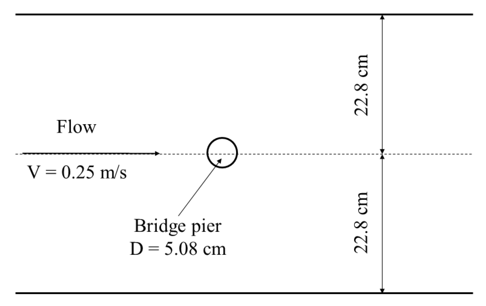
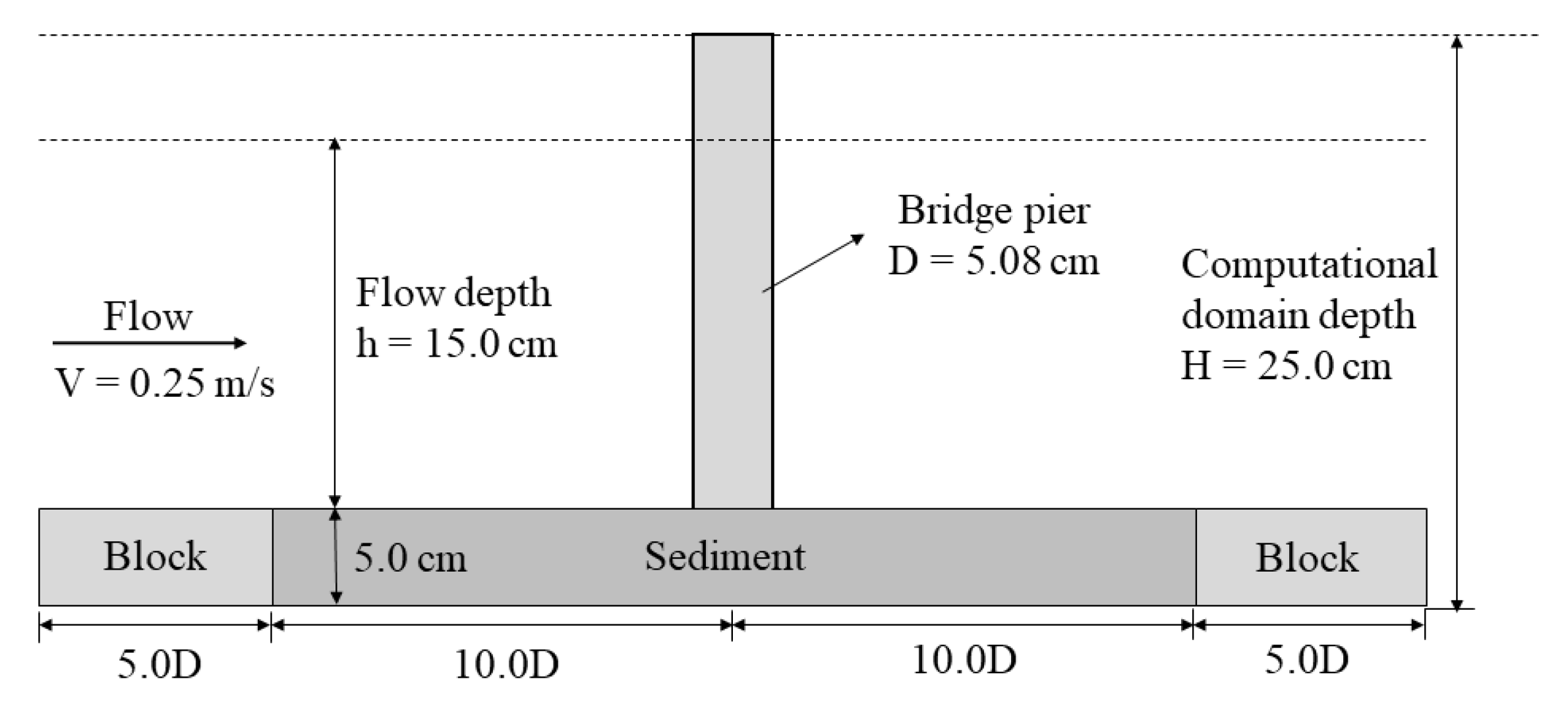
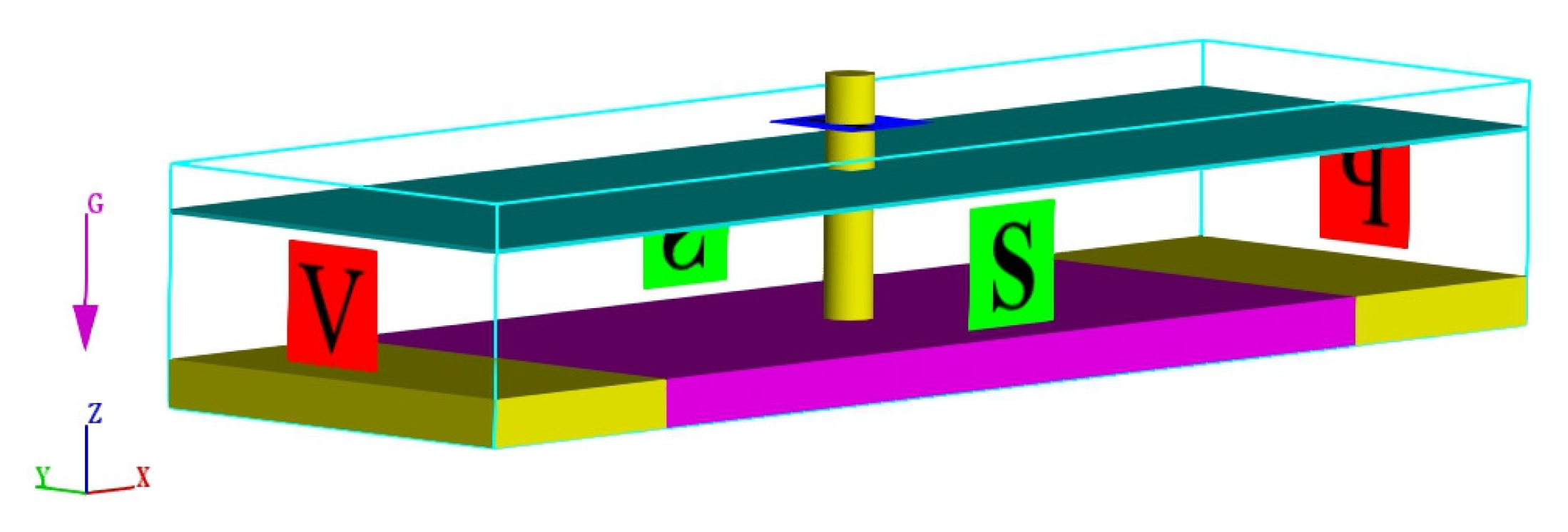
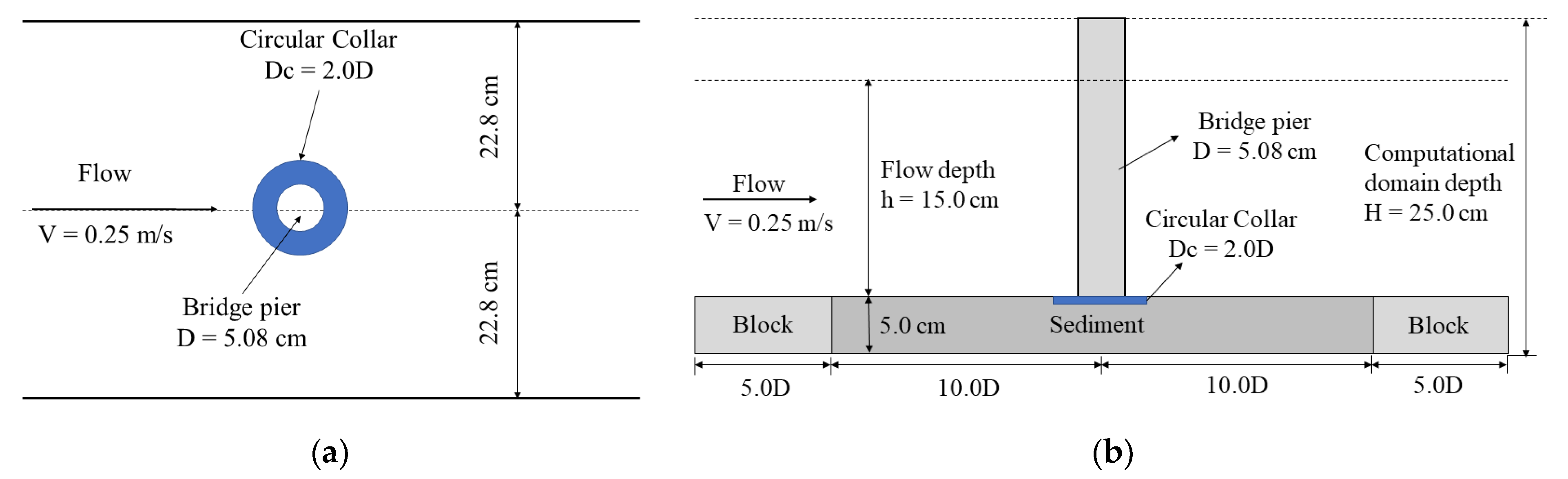
2.3.1. Parameters of the Physical Model

To compare the research results with that of the physical model with a single pier and verify the rationality, the experiment carried out by Melville and Raudkivi [2] is used as a reference in this study. The experiments were carried out in a glass-side flume with a length of 19.0 m, a width of 0.456 m, and a depth of 0.440 m. A cylinder with a diameter of 5.08 cm was used as the bridge pier. The flume was covered by sand with a depth of 13.0 cm. The sand had a uniform grading curve with d₅₀ = 0.385 mm and a specific gravity of 2.65. A uniform flow depth of 15.0 cm and a mean approach velocity of 0.25 m/s were used in the experiment. The experiment lasted for several hours, and the scour hole depth developed rapidly for the first 30 min and developed slowly from that time on. The layout of the flume is shown in Figure 1.

2.3.2. Parameters of the Computational Domain

According to the parameters and the layout of the flume, a computation domain was built in Flow-3D. The height of the domain was 25.0 cm, including a 5.0 cm high sediment, 15.0 cm deep water, and the rest 5.0 cm high in the air. The width of the domain was set as that of the flume. The length of the domain was 30.0D (D is the diameter of the bridge pier) according to Breuer [58] and Sarker [59]. The bridge pier was located in the middle of the domain. A 5.0D length of block was set at both sides of the domain, and 0.033 was set as the Critical Shield number according to the critical shear stress developed by Shields in 1936. The layout of the computation domain is shown in Figure 2, and the parameters of the model are shown in

Table 1. Parameters of the model.

Parameters	Critical Shield Number	Entrainment Coefficient	Bedload Coefficient	Bed Roughness	Static Angle of Repose (°)
Values	0.033	0.018	8	2.5d50	32

.

The upstream boundary was set to an inlet with a velocity of 0.25 m/s, and the downstream boundary was set as Pressure with a flow elevation of 15.0 cm. The top of the domain was set as Pressure with a stagnation pressure of 0.0 Pa, while the surface of the pier was set with a no-slippery condition, and the remaining sides of the domain were set to be symmetrical. The boundary conditions of the model are shown in Figure 3. The fluid (water) is considered incompressible, and the Large Eddy Simulation (LES) model is utilized. The size of the grid is a key factor that affects the simulation results. According to the results of Sarker [59], the flow phenomenon can be completely obtained when the grid size is smaller than D/20 (D is the diameter of the pier). So, the grid size of the computational domain (from 10.0D to 20.0D in the X direction, 0.15 m length in the Y direction at both sides of the pier center, and from −0.05 to 0.15 m in the Z direction) around the bridge pier was set to be 1.0 mm to meet the accuracy requirements of the results. A uniform structured grid block with a mesh size of 3.0 mm in all three directions was used in the remaining computational domain.

To reduce the length of the numerical model in the flow direction, a certain length of the blocks (fixed bed, in yellow in Figure 3) were added at both ends of the sediment (live-bed, in purple in Figure 3) of the numerical model, which can make the flow fully developed and become uniform before entering the live-bed section. It has been proven effective [58,59].

According to the development of the scour hole depth in the experiment, the simulation time was set to be 30 min.

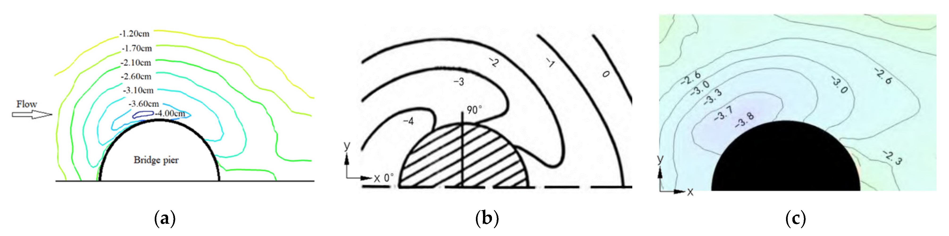
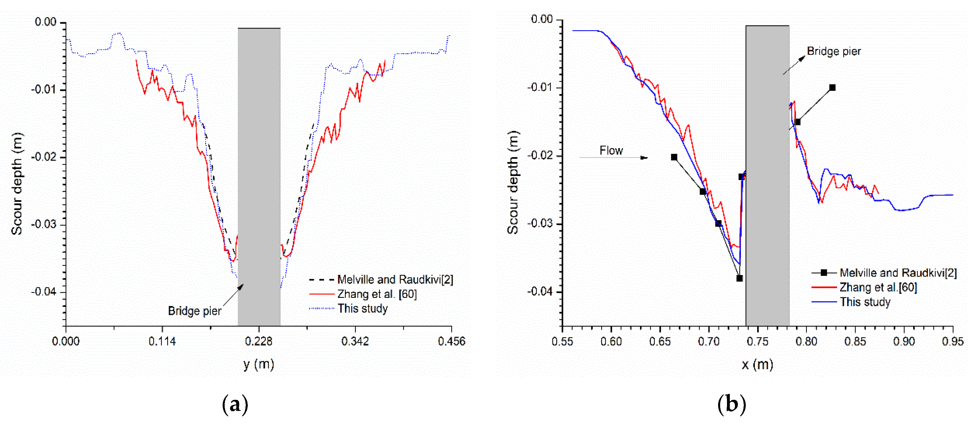
2.3.3. Result of Physical Model Verification

The development of the scour hole around the pier became stable 30 min after the calculation started. The contours of the net height change of the packed sediment were shown in Figure 4a. Measured from the flow direction, the maximum depth of the scour hole is located at around 75°–90° at both sides of the pier. The maximum depth of the scour hole in this study is 4.073 cm and is very close to the results reported by Melville and Raudkivi [2], and Zhang et al. [60], which is 4.0 cm and 3.8 cm respectively, as shown in Figure 4b,c.

As shown in Figure 4, the local scour depth of the pier in this study is close to that reported by Melville and Raudkivi [2], and Zhang et al. [60], but there is a difference in the location of the maximum scour depth. The location of the largest scouring that occurred in Melville’s test was near the front of the pier, while the location of that in this and Zhang’s study are at both sides of the pier. The reason for the difference between this study and others can be summarized as follows.

Firstly, the numerical simulation methods used do not estimate the velocity of turbulent pulsation completely, which makes the local scour depth at the front of the pier conculcated by simulation smaller than that stated by Melville and Raudkivi. Previous studies have shown that the intensity of turbulent pulsation changes with the bluntness of the pier. Simpson’s [61] results have observed that for sharp-angled piers, the maximum scour is mainly located on both sides of the pier, and the scour depth at the front of the pier is very small. For the square pier and cylinder pier, the maximum scour is located within a small range near the front of the pier, which indirectly proves the rationality of the above analysis. The same results were reported by other researchers as well [62,63]. On the other hand, the location error is not only caused by the dullness of the bridge piers but also the shortcomings of the numerical model, such as the settings, the grid size, and so on. The model limitation cannot be eliminated at present due to the method of equation solving (time-averaged, LES, etc.), which has a great influence on the results as well. Although LES uses different solving methods according to the size of the vortex, it still does not match reality completely. No matter how small the grid size is, it does not match the actual situation as well.

Secondly, the sediment on the river bed surface moves by sliding, rolling, and jumping in the actual situation. Transportation has a greater impact on the flow field near the surface of the river bed, especially on the turbulent kinetic energy and the turbulent dissipation rate near the surface of the river bed. Particle–liquid interaction was not considered in the simulation.

Thirdly, the instantaneous shear stress of the river bed surface was used as the only standard for sediment initiation and transportation in simulation code, but it has strong randomness at fields.

Lastly, the difference in the maximum scour depth between this study and other scholars using the CFD code is mainly caused by the boundary conditions. For the boundary condition at the top of the domain, the Pressure with a stagnation pressure of 0.0 Pa means the domain has a free surface that is closer to the actual than the Symmetry, which means the whole domain is filled with the fluid used by other scholars.

The comparisons of scouring characteristics, including the scour depth and the shape, at the cross-section (x = 0.762 m) and longitudinal cross-section (y = 0.228 m) are shown in Figure 5. Figure 5 shows a better coincident between the results of this study and those of the existing studies. The maximum local scouring depth and the shape of the scouring hole in this study are all similar to that of the experimental test.

It can tell that the Large Eddy Simulation (LES) model used in this study is reasonable and accurate. LES can be used for calculating the maximum scouring depth around the bridge pier. For determining the location of the maximum scouring depth, the results of existing studies can be referenced.

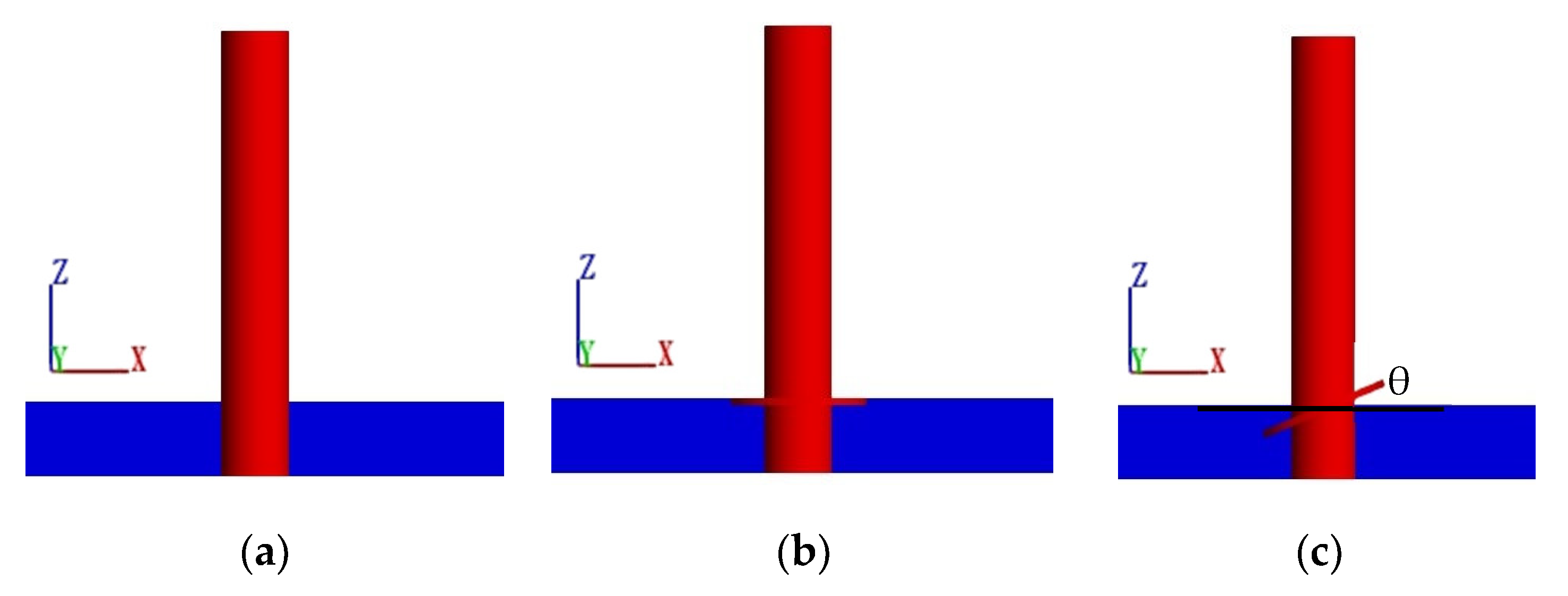
2.4. Parameters of the Model with Circular Collar with Different Tilt Angles

A circular collar with a diameter Dc = 2.0D was added to the pier. The thickness of the circular collar is 0.005 m. It was at the same elevation as the sediment surface on the top, as shown in Figure 6.

In Flow3D, the ratio of the grid size of the computational domain to the average diameter of the sediment (d₅₀) has a great influence on the residuals of the iteration during the simulation, which affects the efficiency of the numerical process. The larger the ratio is, the higher the calculation efficiency. A larger ratio will affect the accuracy of the result, while a smaller ratio will increase the computational workload.

The sediment diameter was reduced to 0.2 mm with a specific gravity of 2.65. So, the ratio increased from about 2.60 (1.00 mm/0.385 mm) to 5.0 (1.00 mm/0.2 mm), which can improve the numerical efficiency. The Critical Shield number was changed to 0.05 according to the diameter of the sediment, while the rest of the parameters and the boundary conditions of the computational domain remained the same.

The circular collar was rotated counterclockwise around the Y-axis in X-Y by five different tilt angles (θ), which were 0°, 5°, 10°, 15°, and 20° (Case 2 to Case 6), respectively. The parameters of each case are shown in

Table 2. Parameters of each case.

Case	1	2	3	4	5	6
Tilt angles of the circular collar (θ)	Without circular collar	0° (horizontal)	5°	10°	15°	20°

. In addition to these five cases, Case 1 without a circular collar was also simulated. The simulation models of Case 1, Case 2, and Case 6 are shown in Figure 7.

3. Results and Discussion

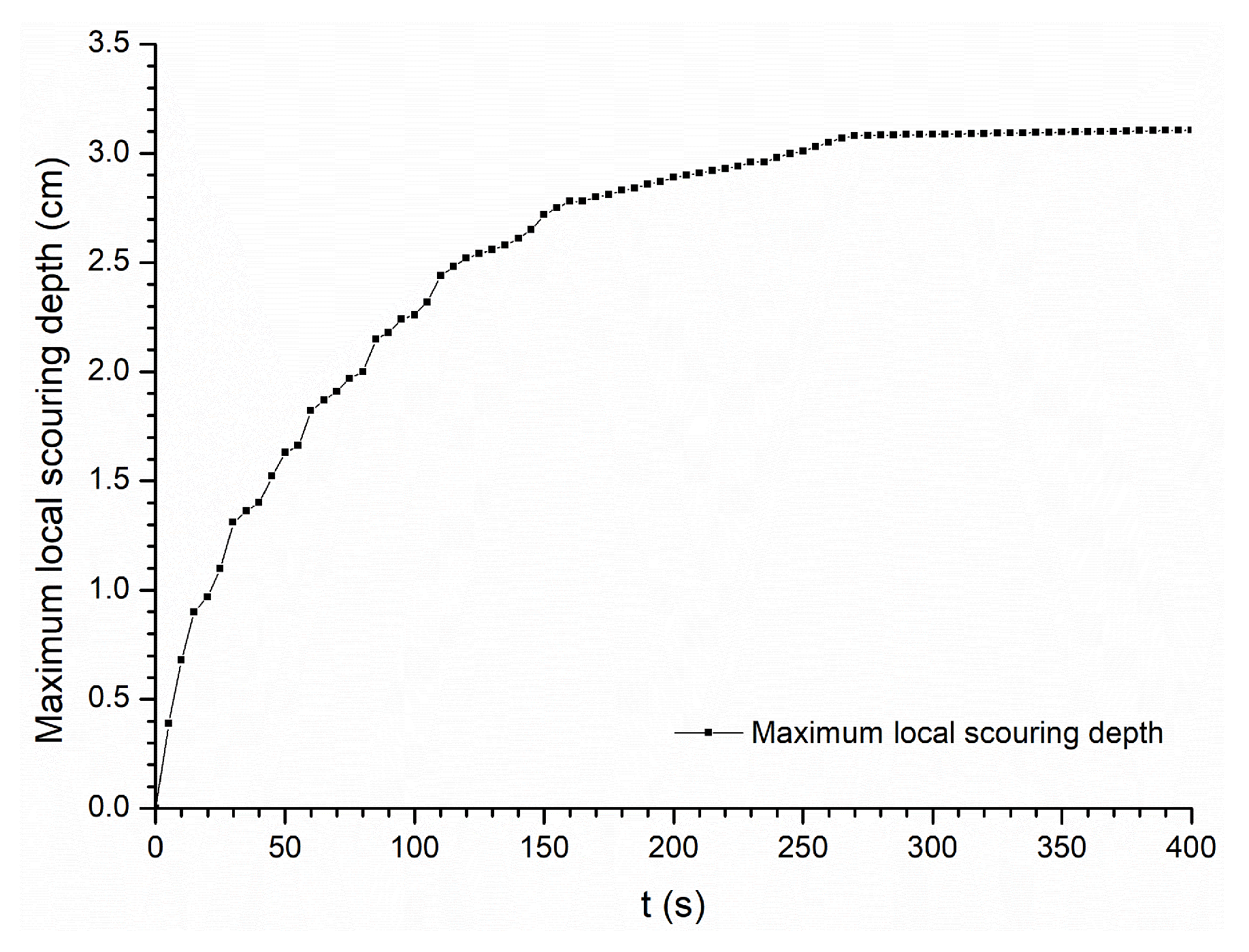
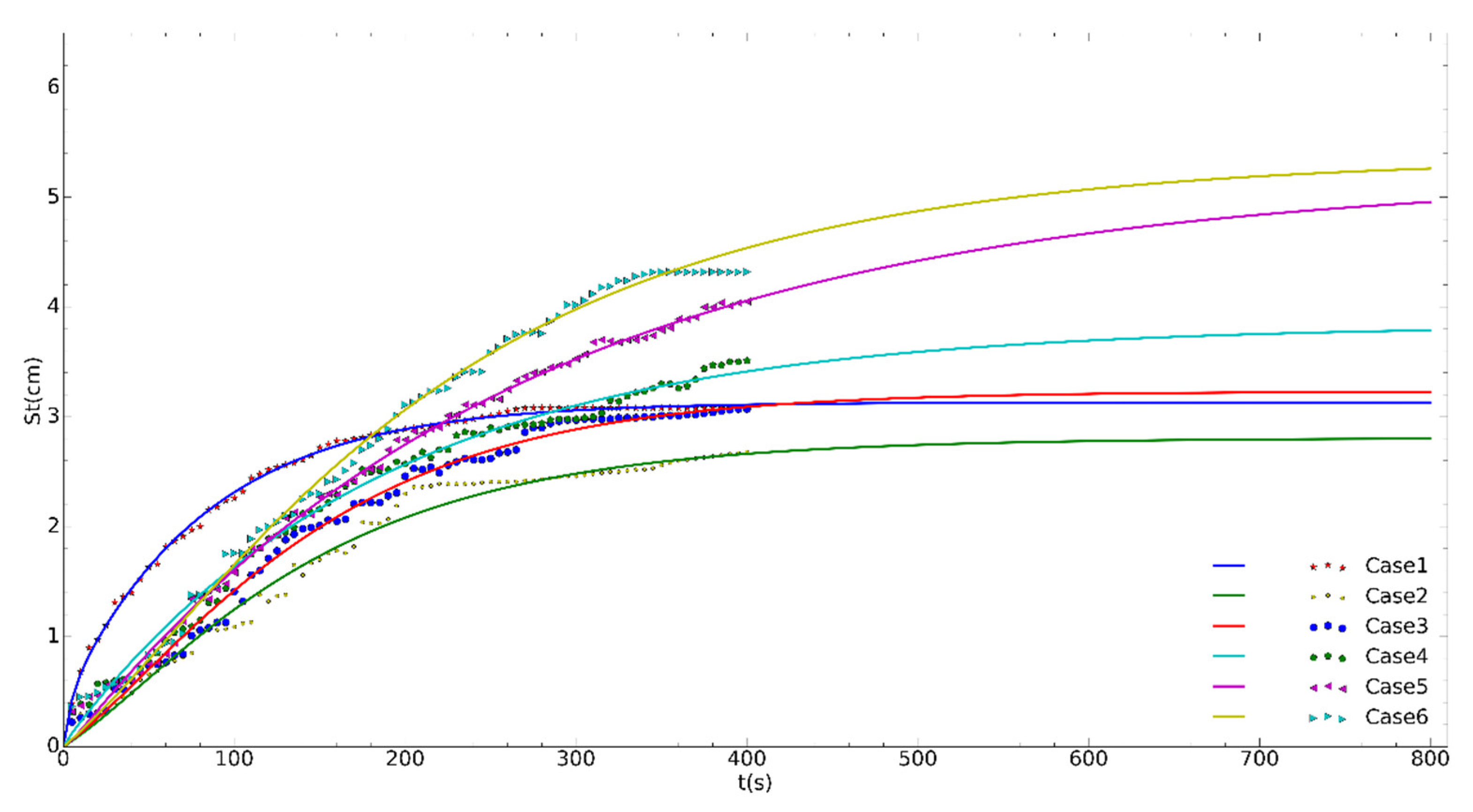
3.1. The Maximum Scouring Depth in Each Case

The maximum scouring depth of Case 1 every 10 s was plotted in Figure 8.

As shown in Figure 8, the maximum local scouring depth in Case 1 increases rapidly in the early stage (in 150 s); then, it slowed down (150 to 260 s) and became stable after 260 s. This scour development meets the law of the local scouring development. Therefore, 400 s was used in this simulation.

Earlier studies by Sheppard [64] showed that the relationship between the maximum local scour depth (S_t) and the scour time (t) can be expressed as shown in Equation (14):

$$S_t=a\left[1-\exp \left(-bt\right)\right]+c\left[1-\exp \left(-dt\right)\right]$$

(14)

where a, b, c, and d are all parameters.

Using the function above, the curves of maximum local scour depths in the six cases in 800 s (the fitted curve) are shown in Figure 9, and the parameters in the function of each case are shown in

Table 3. The parameters in the function.

Cases	a	b	c	d	Correlation Coefficient
1	2.7463	0.0121	0.3846	0.2257	0.9998
2	3.8053	0.0082	−0.9999	0.0215	0.9925
3	6.2384	0.0094	−3.0090	0.0157	0.9968
4	3.8130	0.0055	0.0213	0.3054	0.9954
5	5.2669	0.0038	−0.0575	0.2281	0.9980
6	6.6349	0.0052	−1.2693	0.0170	0.9976

.

As shown in Table 3, the correlation coefficients of all cases are very close to 1.0, which means the curves created by the function fit the experimental data very well. So, the curves can be used to predict the maximum local scour depth at the scour equilibrium.

As shown in Figure 9, at the scour equilibrium, the smaller the tilt angle of the collar is, the better the effect on local scour reduction. Case 2 is the best case for reducing the maximum local scouring depth. It can reduce the maximum local scouring depth by about 10%. The maximum local scour depth of Case 3 is slightly larger than that of Case 1 by about 3.5%. The maximum local scour depth of Case 4, Case 5, and Case 6 are all greater than that of Case 1 by 22.6%, 61.29%, and 71.0%. It shows that with the increases of the tilt angle, the effect on reducing the local scour depth decreases gradually and is even counterproductive.

The tilt angle of the circular collar has a great impact on the local scour process. In each case, the circular collar has a similar effect on local scour depth reduction at the early stage of scouring, especially in the first 100 s. The effect decreases with the increase of the tilt angle afterward. If the duration of scouring is short, the scour depth can be reduced effectively in all cases. When the tilt angle grows greater, the length of time during which the local scouring depth can be reduced gets shorter. The length of the protection time of Case 6, Case 5, Case 4, and Case 3 is about 185 s, 220 s, 295 s, and 400 s. If the scouring lasted longer than that duration, the local scouring depth got intensified.

The main reason for the decrease of the maximum local scouring depth at the early stages is that the circular collar restricts the development and scale of the horseshoe vortices below the circular collar compared to Case 1. The scour depth and vectors at x = 0.762 m (the center of the pier) at t = 400 s of each case are shown in Figure 10. The tilt angle affects directly to the effect of the circular collar restriction on the development of the horseshoe vortex. The smaller the angle is, the more effective the restriction.

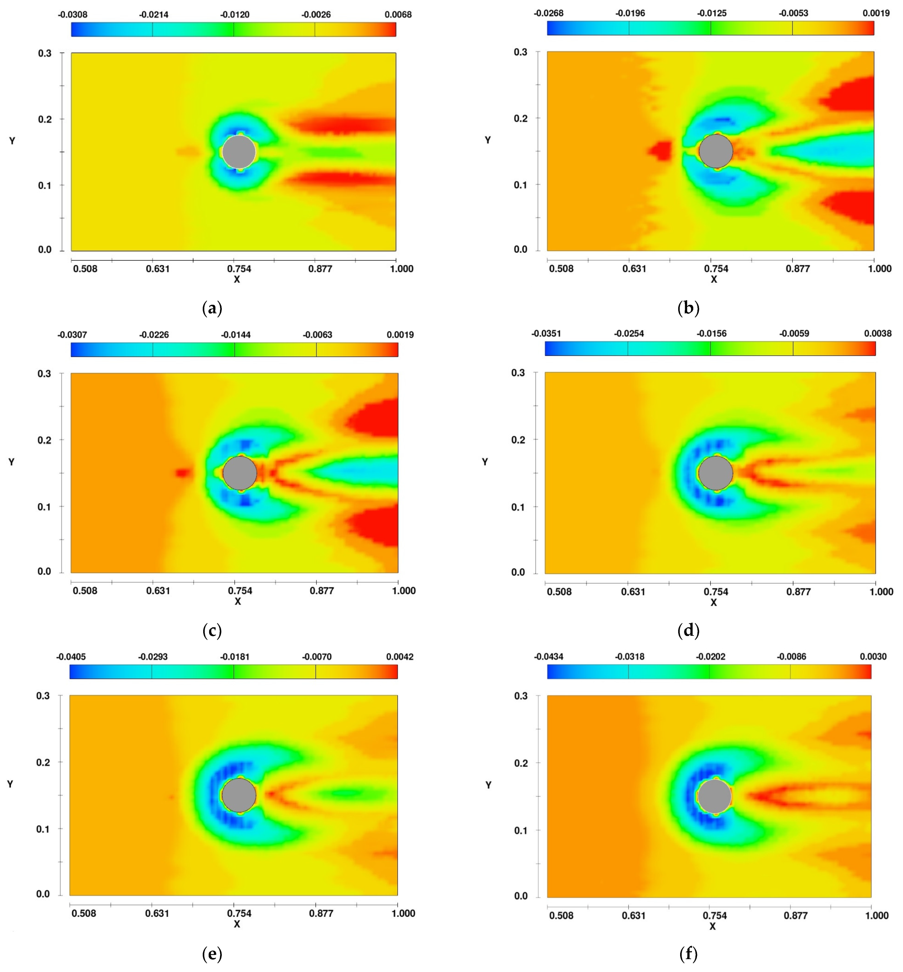
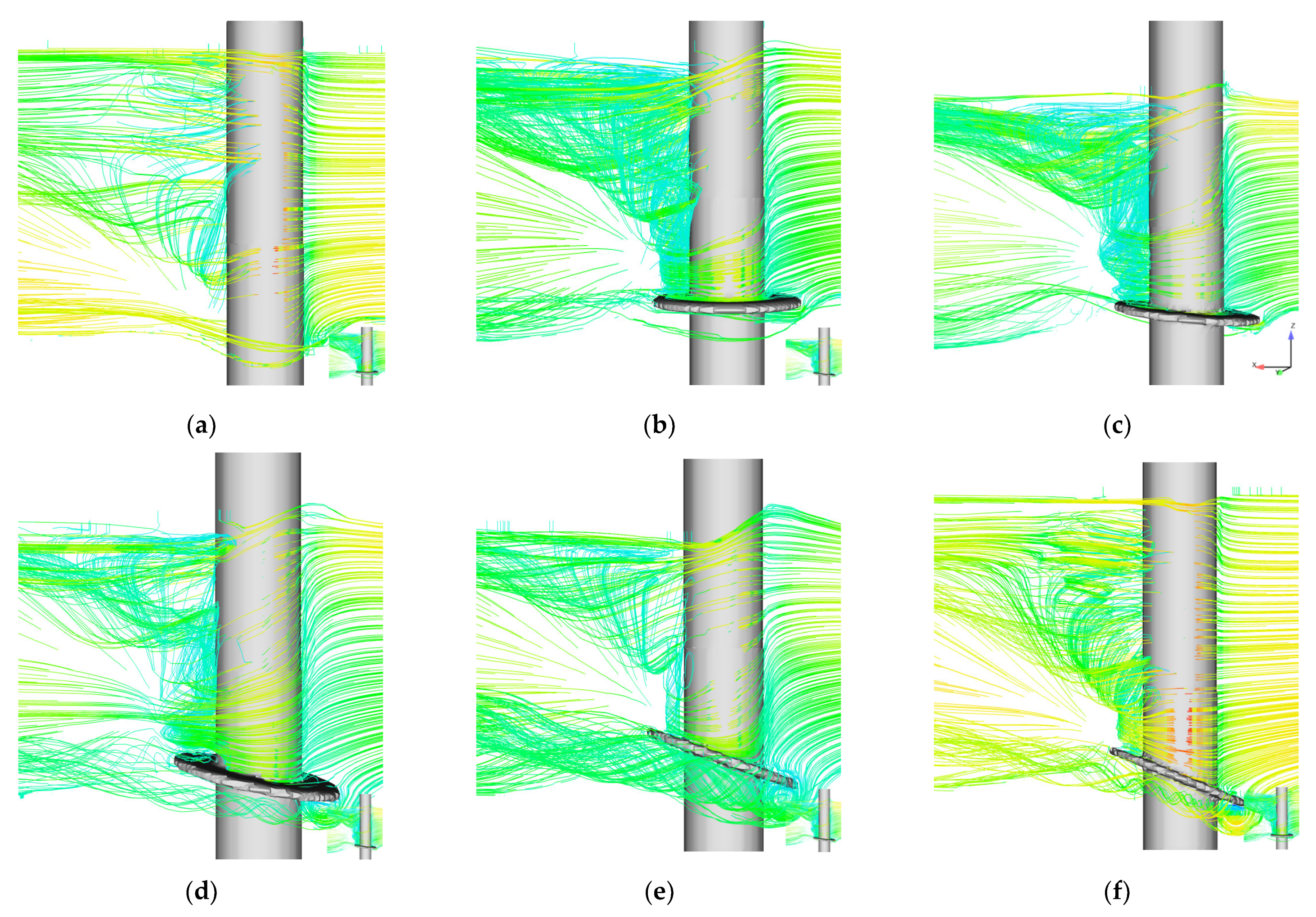
3.2. The Topography of Each Case

The top views of the scour topography at t = 400 s in each case are shown in Figure 11.

As shown in Figure 11, the tilt angle of the circular collar has a great influence on the scour topography compared with Case 1.

After it reached scour equilibrium, the location of the maximum scouring depth of Case 1 was in the range around 45–75° (the angle is measured clockwise from the flow direction) on both sides of the pier. Those of Case 2 and Case 3 were around 90–115° on both sides of the pier. In Case 4, Case 5, and Case 6, the location of the maximum scour depth was around −115–115°. It shows that when the tilt angle increase, the location of the maximum local scour depth moves downstream of the flow, and the range of the scour depth that is close to the maximum local scouring increases significantly.

The range of the scouring hole around the pier in each case with the circular collar increased significantly compared to Case 1. The shapes of the scouring holes were similar, but the area with larger scouring depth increased gradually with the increase of the tilt angle. Compared with Case 1, the area of the scour hole in the other five cases expanded downstream by about 1.5D and expands laterally by about 0.8D. The main reason for the range expansion of the scouring hole is that the diameter of the circular collar is twice the diameter of the pier, and those two parts form a larger structure, which increases the range of the local scouring.

The tilt angle of the circular collar has a great effect on the topography downwards the pier in each case, especially the shape and the location of the scouring and siltation. Compared with Case 1, the topography downwards the pier was 1.0D in cases with circular collar changes to siltation from scouring. The smaller the tilt angle was, the higher the siltation. The topography downwards of the pier was changed from scouring to siltation with the increase of the tilt angle. The shape of siltation was changed from a long-narrow rectangle to an equilateral triangle, which was about 2.5D downwards the front of the former siltation area.

To analyze the causes of the topographic changes downstream the bridge piers, the streamlines (colored by the velocity) at y = 0.15 m and t = 400 s of each case are shown in Figure 12.

As shown in Figure 12, the circular collar has a great influence on the vortex system generated when the flow bypasses the pier compared with Case 1. The vortex system is divided into two parts: one above the circular collar and the other one below it. Due to the constraint of the circular collar and the pier, the scale of the vortex system above the circular collar is smaller than that in Case 1, and it increased continuously when it raised to the free surface. This is the main cause of the siltation in a range of about 1.0D behind the pier in other cases. With the increase of the tilt angle of the circular collar, the blocking area of the circular collar to the flow increased gradually. More and more horseshoe vortexes were generated by the falling flows when they met the surface of the circular collar, which aggravated the depth and progress of the local scour in front of the pier. With the development of the local scouring hole around the pier, the number of streamlines passing below the circular collar increased, and the strength of the vortex below the circular collar increased rapidly, which causes the topography in 1.0D behind the pier to be changed from siltation to scouring gradually.

4. Conclusions

This research explores the effects of the circular collar with tilt angles (counterclockwise around the direction of the channel cross-section) on the local scour depth around a single cylindrical pier in clear-water based on Large Eddy Simulation. The main findings are summarized below.

• At the scour equilibrium, Case 2 (θ = 0°) is the best for reducing the local scour depth, and it can reduce the maximum local scouring depth by about 10%. With the increases of the tilt angle, the effect on reducing the local scour depth decreases gradually and is even counterproductive.
• At the early stage of scouring, cases with a circular collar prove that the circular collar can reduce the scour depth significantly. The smaller the tilt angle is, the more obvious effect on the scouring depth reduction.
• When the tilt angle is less than 5°, the location of the maximum local scouring depth is around 90 to 115° (the angle is measured clockwise from the flow direction) on both sides of the pier. The location of the maximum scour depth is around −115° to 115° when the tilt angle is larger than 5°, and the range of the local scour depth that is close to the maximum local scouring depth increases significantly when the tilt angle increases.
• Compared to Case 1, the area of the scour hole expands downstream by about 1.5D and expands laterally by about 0.8D. The topography downwards the pier in 1.0D in cases with a circular collar is changed to siltation from scouring. The smaller the tilt angle is, the higher the siltation. The topography downwards the pier is changed from scouring to siltation with the increase of the tilt angle, and the shape of siltation changes from a long-narrow rectangle to an equilateral triangle, which is about 2.5D downwards from the front of the former siltation area.

References

1. Breusers, H.N.C.; Nicollet, G.; Shen, H.W. Local scour around cylindrical piers. J. Hydraul. Res. 1977, 15, 211–252. [Google Scholar] [CrossRef]
2. Melville, B.W.; Raudkivi, A.J. Flow characteristics in local scour at bridge piers. J. Hydraul. Res. 1977, 15, 73–380. [Google Scholar] [CrossRef]
3. Gao, D.G. Road and Bridge Flood Damage Prevention; China Communications Press: Beijing, China, 2002. [Google Scholar]
4. Hunt, E.B. Monitoring Scour Critical Bridges; Transportation Research Board: Washington, DC, USA, 2009; pp. 1–10. [Google Scholar]
5. Yi, R.Y. Causes and Risk Analysis of Bridge Collapse Accidents. Maint. Manag. 2016, 4, 22–26. [Google Scholar]
6. Melville, B.W. Local Scour at Bridge Pier Site. Ph.D. Thesis, School of Engineering, University of Auckland, Auckland, New Zealand, 1975. [Google Scholar]
7. Chiew, Y.M.; Melville, B.W. Local scour around bridge piers. J. Hydraul. Res. 1987, 25, 15–26. [Google Scholar] [CrossRef]
8. Melville, B.W.; Sutherland, A.J. Design method for local scour at bridge piers. J. Hydraul. Eng. 1988, 114, 1210–1226. [Google Scholar] [CrossRef]
9. Melville, B.W. The Physics of Local Scour at Bridge Piers. In Proceedings of the 4th International Conference on Scour and Erosion (ICSE-4), Tokyo, Japan, 5–7 November 2008. [Google Scholar]
10. Deng, L.; Cai, C.S. Bridge Scour: Prediction, Modeling, Monitoring, and Countermeasures-Review. Pract. Period. Struct. Des. Constr. 2010, 15, 125–134. [Google Scholar] [CrossRef] [Green Version]
11. Negm, A.M.; Gamal, M.; Moustafa, Y.M.; Fathy, A.A. Optimal shape of collar to minimize local scour around bridge piers. In Proceedings of the Thirteenth International Water Technology Conference IWTC13, Hurghada, Egypt, 1 January 2009; pp. 1–13. [Google Scholar]
12. Ardeshiri, A.M.; Mojtaba, S. Experimental Study on Lozenge Collar Affection in Reduce Amount of Scouring Around Bridge Piers. J. River Eng. 2014, 2, 7–11. [Google Scholar]
13. Jahangirzadeh, A.; Hossein, B.; Shatirah, A.; Hojat Karami, S.N.; Shahaboddin, S. Experimental and Numerical Investigation of the Effect of Different Shapes of Collars on the Reduction of Scour around a Single Bridge Pier. PLoS ONE 2014, 9, e98592. [Google Scholar] [CrossRef] [PubMed]
14. Chen, S.C.; Samkele, T.; Wu, T.Y.; Chan, H.C.; Chou, H.T. A Hooked-Collar for Bridge Piers Protection: Flow Fields and Scour. Water 2018, 10, 1251. [Google Scholar] [CrossRef] [Green Version]
15. Roulund, A.; Sumer, B.M.; Fredsøe, J.; MicheIsen, J. Numerical and experimental investigation of flow and scour around a circular pile. J. Fluid Mech. 2005, 534, 351–401. [Google Scholar] [CrossRef]
16. Abouzeid, G.; Mohamed, H.I.; Ali, S.M. 3-D numerical simulation of flow and clear water scour by interaction between bridge piers. J. Eng. Sci. 2007, 35, 891–907. [Google Scholar] [CrossRef]
17. Esmaeili, T.; Dehghani, A.A.; Zahiri, A.R.; Suzuki, K. 3D numerical simulation of scouring around bridge piers (Case study: Bridge 524 crosses the Tanana River). World Acad. Sci. Eng. Technol. 2009, 34, 1028–1032. [Google Scholar]
18. Huang, W.; Yang, Q.; Xiao, H. CFD modeling of scale effects on turbulence flow and scour around bridge piers. Comput. Fluids 2009, 38, 1050–1058. [Google Scholar] [CrossRef]
19. Zhu, Z.; Liu, Z. Three-dimensional numerical simulation for local scour around cylindrical bridge pier. China J. Highw. Transp. 2011, 24, 43–48. [Google Scholar]
20. Khosronejad, A.; Kang, S.; Sotiropoulos, F. Experimental and computational investigation of local scour around bridge piers. Adv. Water Resour. 2012, 37, 73–85. [Google Scholar] [CrossRef]
21. Xiong, W.; Wang, J.; Ye, J. Effect of pier structures on local scour 3D development. J. Southeast Univ. (Nat. Sci. Ed.) 2014, 44, 155–161. [Google Scholar]
22. Ahmad, N.; Bihs, H.; Kamath, A.; Arntsen, Ø.A. Three-dimensional CFD modeling of wave scour around side-by-side and triangular arrangement of piles with REEF3D. Procedia Eng. 2015, 116, 683–690. [Google Scholar] [CrossRef] [Green Version]
23. Ghasemi, M.; Soltani-Gerdefaramarzi, S. The scour bridge simulation around a cylindrical pier using Flow-3D. J. Hydrosci. Environ. 2017, 1, 46–54. [Google Scholar]
24. Alemi, M.; Maia, R. Numerical simulation of the flow and local scour process around single and complex bridge piers. Int. J. Civ. Eng. 2018, 16, 475–487. [Google Scholar] [CrossRef]
25. Jia, Y.; Altinakar, M.; Guney, M.S. Three-dimensional numerical simulations of local scouring around bridge piers. J. Hydraul. Res. 2018, 56, 351–366. [Google Scholar] [CrossRef]
26. Svsndl, P.; Suresh, K.N. Simulation of flow behavior around bridge piers using ANSYS–CFD. Int. J. Eng. Sci. Invent. (IJESI) 2018, 7, 13–22. [Google Scholar]
27. Pang, A.; Skote, M.; Lim, S.Y. A numerical approach for determining equilibrium scour depth around a mono-pile due to steady currents. Appl. Ocean Res. 2016, 57, 114–124. [Google Scholar] [CrossRef]
28. Hamidi, A.; Siadatmousavi, S.M. Numerical simulation of scour and flow field for different arrangements of two piers using SSIIM model. Ain Shams Eng. J. 2017, 9, 2415–2426. [Google Scholar] [CrossRef]
29. Rodi, W. Comparison of LES and RANS calculations of the flow around bluff bodies. J. Wind Eng. Ind. Aerodyn. 1997, 71, 55–75. [Google Scholar] [CrossRef]
30. Sagaut, P. Large Eddy Simulation for Incompressible Flows; Springer: Berlin/Heidelberg, Germany, 1988. [Google Scholar]
31. Rodi, W.; Ferziger, J.H.; Breuer, M.; Pourquia, M. Proc. Workshop on Large-Eddy Simulation of Flows Past Bluff Bodies; Cambridge University Press: Rottach-Egern, Germany, 1995. [Google Scholar]
32. Rodi, W.; Ferziger, J.H.; Breuer, M.; Pourquia, M. Status of large-eddy simulation: Results of a workshop. J. Fluids Eng. 1997, 119, 248–262. [Google Scholar] [CrossRef]
33. Breuer, M. Large-eddy simulation of the subcritical flow past a circular cylinder: Numerical and modeling aspects. Int. J. Numer. Meth. Fluids 1998, 28, 1281–1302. [Google Scholar] [CrossRef]
34. Van Balen, W.; Uijttewaal, W.S.J.; Blanckaert, K. Large-eddy simulation of a mildly curved open-channel flow. J. Fluid Mech. 2009, 630, 413–442. [Google Scholar] [CrossRef] [Green Version]
35. van Balen, W.; Blanckaert, K.; Uijttewaal, W.S.J. Analysis of the role of turbulence in curved open-channel low at different water depths by means of experiments, LES and RANS. J. Turbul. 2010, 11, N12. [Google Scholar] [CrossRef]
36. Hinterberger, C.; Froehlich, J.; Rodi, W. Three-dimensional and depth-averaged large-eddy simulations of some shallow water flows. J. Hydraul. Eng.-ASCE 2007, 133, 857–872. [Google Scholar] [CrossRef]
37. Han, D.; Fang, H.W.; Bai, J. A coupled 1-D and 2-D channel network mathematical model used for flow calculations in the middle reaches of the Yangtze River. J. Hydrodyn. 2011, 23, 521–526. [Google Scholar] [CrossRef]
38. Armenio, V. Large-eddy simulation in hydraulic engineering: Examples of laboratory-scale numerical experiments. J. Hydraul. Eng. 2017, 143, 03117007. [Google Scholar] [CrossRef]
39. Dhamankar, N.S.; Blaisdell, G.A.; Lyrintzisz, A.S. An overview of turbulent inflow boundary conditions for large-eddy simulations. AIAA J. 2018, 56, 1317–1334. [Google Scholar] [CrossRef]
40. Keating, A.; Piomelli, U.; Balaras, E. A priori and a posteriori test of inflow conditions for large-eddy simulation. Phys. Fluids 2004, 16, 4696–4712. [Google Scholar] [CrossRef]
41. Khosronejad, A.; Hansen, A.T.; Kozarek, J.L. Large-eddy simulation of turbulence and solute transport in a forested headwater stream. J. Geophys. Res. Earth Surf. 2016, 121, 146–167. [Google Scholar] [CrossRef] [Green Version]
42. Le, T.; Khosronejad, A.; Bartelt, N. Large-eddy simulation of the Mississippi River under base-flow condition: Hydrodynamics of a natural diffluence-confluence region. J. Hydraul. Res. 2018, 57, 836–851. [Google Scholar] [CrossRef]
43. Van Balen, W.; Uijttewaal, W.S.J.; Blanckaert, K. Large-eddy simulation of a curved open-channel flow over topography. Phys. Fluids 2010, 22, 075108. [Google Scholar] [CrossRef] [Green Version]
44. Bai, J.; Fang, H.W.; Stoesser, T. Transport and deposition of fine sediment in open channels with different aspect ratios. Earth Surf. Process. Landf. 2012, 38, 591–600. [Google Scholar] [CrossRef]
45. Chou, Y.J.; Fringer, O.B. Modeling dilute sediment suspension using large-eddy simulation with a dynamic mixed model. Phys. Fluids 2008, 20, 115103. [Google Scholar] [CrossRef] [Green Version]
46. Khosronejad, A.; Angelidis, D.; Bagherizadeh, E. A comparative study of rigid-lid and level-set methods for LES of open-channel flows: Morphodynamics. Environ. Fluid Mech. 2020, 20, 145–164. [Google Scholar] [CrossRef]
47. Khosronejad, A.M.; Ghazan, D.; Angelidis, E. Comparative hydrodynamic study of rigid lid and level set methods for LES of open-channel flow. J. Hydraul. Eng. 2019, 145, 04018077. [Google Scholar] [CrossRef]
48. McCoy, A.; Constantinescu, G.; Weber, L.J. Exchange processes in a channel with two vertical emerged obstructions. Flow Turbul. Combust. 2006, 77, 97–126. [Google Scholar] [CrossRef]
49. McCoy, A.; Constantinescu, G.; Weber, L.J. Numerical investigation of flow hydrodynamics in a channel with a series of groynes. J. Hydraul. Eng. 2008, 134, 157–172. [Google Scholar] [CrossRef]
50. Constantinescu, G.; Sukhodolov, A.; McCoy, A. Mass exchange in a shallow channel flow with a series of groynes: LES study and comparison with laboratory and field experiments. Environ. Fluid Mech. 2009, 9, 587–615. [Google Scholar] [CrossRef]
51. Brevis, W.; Garcia-Villalba, M.; Nino, Y. Experimental and large eddy simulation study of the flow developed by a sequence of lateral obstacles. Environ. Fluid Mech. 2014, 14, 873–893. [Google Scholar] [CrossRef]
52. Kirkil, G.; Asce, S.M.; Constantinescu, S.G. Coherent structures in the flow field around a circular cylinder with scour hole. J. Hydraul. Eng.-ASCE 2008, 134, 572–587. [Google Scholar] [CrossRef]
53. Koken, M.; Constantinescu, G. An investigation of the flow and scour mechanisms around isolated spur dikes in a shallow open channel: 1. Conditions corresponding to the initiation of the erosion and deposition process. Water Resour. Res. 2008, 44. [Google Scholar] [CrossRef]
54. Koken, M.; Constantinescu, G. An investigation of the flow and scour mechanisms around isolated spur dikes in a shallow open channel: 2. Conditions corresponding to the final stages of the erosion and deposition process. Water Resour. Res. 2008, 44. [Google Scholar] [CrossRef]
55. Chandara, M. Numerical Investigation of Bridge-Pier Scour Using Flow-3D. Master’s Thesis, Northwest A&F University, Yang Ling, China, 2019. [Google Scholar]
56. Dey, S. Bed-Load Transport. In Fluvial Hydrodynamics; Springer: Berlin/Heidelberg, Germany, 2014. [Google Scholar]
57. Flow-3D User’s Manuals; Flow Science, Inc.: Santa Fe, NM, USA, 2009.
58. Breuer, M. Numerical and modeling influences on large-eddy simulations for the flow past a circular cylinder. Int. J. Heat Fluid Flow 1998, 19, 512–521. [Google Scholar] [CrossRef]
59. Sarker, M.A. Flow measurement around scoured bridge piers using Acoustic-Doppler Velocimetry (ADV). Flow Meas. Instrum. 1998, 9, 217–227. [Google Scholar] [CrossRef]
60. Zhang, S.; Yin, J.; Zhang, G. Large-eddy simulation on local scour of cylindrical piers based on Flow-3D. J. Sediment Res. 2020, 45, 67–73. [Google Scholar]
61. Simpson, R.L. Junction flows. Annu. Rev. Fluid Mech. 2001, 33, 415–430. [Google Scholar] [CrossRef]
62. Fleming, J.; Simpson, R.; Devenport, W. An experimental study of a turbulent wing-body junction and wake flow. Exp. Fluids 1993, 14, 366–378. [Google Scholar] [CrossRef] [Green Version]
63. Olcmen, M.; Simpson, R. Influence of wing shapes on surface pressure fluctuations at wing-body junctions. AIAA J. 1994, 32, 615. [Google Scholar] [CrossRef]
64. Sheppard, D.M.; Odeh, M.; Glasser, T. Large Scale Clear-Water Local Pier Scour Experiments. J. Hydraul. Eng. 2004, 130, 957–963. [Google Scholar] [CrossRef]
Figure 1. The layout of the flume (top view).
Water 13 03281 g001
Figure 2. The layout of the computational domain (side view).
Water 13 03281 g002
Figure 3. The boundary conditions of the model.
Water 13 03281 g003
Figure 4. The contours of packed sediment net height change (unit: cm). (a) In this study. (b) Melville and Raudkivi [2]. (c) Zhang et al. [60].
Water 13 03281 g004
Figure 5. The comparison of scour characteristics with existing results. (a) Scour characteristics at x = 0.762 m. (b) Scour characteristics at y = 0.228 m.
Water 13 03281 g005
Figure 6. The layout of the model with a circular collar. (a) The layout of the flume (top view). (b) The layout of the computational domain (side view).
Water 13 03281 g006
Figure 7. The models of Case 1, Case 2, and Case 6. (a) Case 1 (without circular collar). (b) Case 2 (θ = 0°). (c) Case 6 (θ = 20°).
Water 13 03281 g007
Figure 8. The maximum local scouring depth of Case 1 every 10 s.
Water 13 03281 g008
Figure 9. The fitted curve of the maximum scouring depth of each case in 800 s.
Water 13 03281 g009
Figure 10. The scouring depth and vectors at x = 0.762 m (the center of the pier, t = 400 s) of each case (unit: m). (a) Case 1 (without circular collar). (b) Case 2 (θ = 0°). (c) Case 3 (θ = 5°). (d) Case 4 (θ = 10°). (e) Case 5 (θ = 15°). (f) Case 6 (θ = 20°).
Water 13 03281 g010
Figure 11. The top view of the topography in each case at t = 400 s (unit: m). (a) Case 1 (without circular collar). (b) Case 2 (θ = 0°). (c) Case 3 (θ = 5°). (d) Case 4 (θ = 10°). (e) Case 5 (θ = 15°). (f) Case 6 (θ = 20°).
Water 13 03281 g011
Figure 12. The streamline (colored by the velocity) at y = 0.15 m and t = 400 s of each case. (a) Case 1 (without circular collar). (b) Case 2 (θ = 0°). (c) Case 3 (θ = 5°). (d) Case 4 (θ = 10°). (e) Case 5 (θ = 15°). (f) Case 6 (θ = 20°).
Water 13 03281 g012