
A Permeability Estimation Method Based on Elliptical Pore Approximation
by
 , , ,
, , ,
Shuaishuai Wei
1 ,
,
Kun Wang
2,*,
Huan Zhang
1,
Junming Zhang
2,
Jincheng Wei
1,
Wenyang Han
1 and
Lei Niu
1 1
Shandong Transportation Institute, Jinan 250102, China
2
College of Energy and Mining Engineering, Shandong University of Science and Technology, Qingdao 266590, China
*
Author to whom correspondence should be addressed.
Water 2021, 13(22), 3290; https://doi.org/10.3390/w13223290
Submission received: 17 September 2021
/
Revised: 14 November 2021
/
Accepted: 15 November 2021
/
Published: 20 November 2021
(This article belongs to the Special Issue Environmental Fluid Dynamics and Modeling)
Abstract
:Digital rock images may capture more detailed pore structure than the traditional laboratory methods. No explicit function can correlate permeability accurately for flow within the pore space. This has motivated researchers to predict permeability through the application of numerical techniques, e.g., using the finite difference method (FDM). However, in order to get better permeability calculation results, the grid refinement was needed for the traditional FDM and the accuracy of the traditional method decreased in pores with elongated cross sections. The goal of this study is to develop an improved FDM (IFDM) to calculate the permeabilities of digital rock images with complex pore space. An elliptical pore approximation method is invoked to describe the complex pore space. The permeabilities of four types of idealized porous media are calculated by IFDM. The calculated results are in sound agreement with the analytical solutions or semi-empirical solutions. What’s more, the permeabilities of the digital rock images after grid coarsening are calculated by IFDM in three orthogonal directions. These results are compared with the previously validated lattice-Boltzmann method (LBM), which indicates that the predicted permeabilities calculated by IFDM usually agree with permeabilities calculated by LBM. We conclude that the presented IFDM is suitable for complex pore space.
1. Introduction
Permeability describes how easily fluid can flow through rock. The accurate prediction of permeability on small rock samples has important applications in petroleum engineering, environmental studies, hydrogeology and coal mining [1,2,3]. However, determining the permeability by traditional physical experiments usually costs a lot of time and money. Three dimensional (3D) images of rock samples, obtained with micro computed tomography (micro-CT), may be useful to estimate permeability. CT imaging is an effective tool for describing mechanical and transport behaviors of digital rocks [4,5,6,7,8,9,10]. The quality of the pore network extracted plays a significant role in the prediction of the permeability, and the permeability is then calculated mathematically from physical principles. Many researchers have studied multiphase flow systems [11,12,13,14,15,16], but in this study, we focus on the single-phase flow system. The lattice Boltzmann method (LBM) [17,18,19,20] is relatively more commonly used for simulating fluid flow phenomena at the pore scale and is a straightforward method. However, this method is time-consuming and requires the use of massively parallel computing approaches [21]. The finite difference method (FDM) is an effective tool to calculate the permeability [1,22,23,24,25,26,27,28]. The FDM can save much computational time relative to the LBM with similar results [29].
Most porous media are very complex, which makes it very difficult to describe their internal structure accurately. In order to develop theoretical models of various transport processes, an approximation of the pore space should be adopted. The pore-scale correlations found in Finney packing may exist in granular porous media [30,31,32,33], but these correlations may be not suitable for carbonate digital rock images. Javadpour and Pooladi-Darvish [34] presented a two-dimensional representation of a network of unit cells that are connected by branches to investigate the effects of oil viscosity on gas mobility in porous media. Raoof and Hassanizadeh [35] presented a 3D network representing porous media with coordination number of 26. Coordination number is defined as the number of bonds (or pore throats) associated to a site (or pore body) in the network. Shabro et al. [27] presented a finite difference approximation method to calculate the permeability of digital rock image, and they applied a geometrical pore approximation to describe the irregular pore space. However, the geometrical pore approximation is not suitable for elongated cross sections, because the irregular cross sections are partitioned into the form of many interconnecting cylindrical pores. Wang et al. [36] applied a pore network model combined with CT imaging to simulate and calculated the flow properties of methane hydrate. An et al. [37] adopted a random pore network model to simulate two-phase flow. A maximal ball algorithm was adopted to simulate the pore network [38]. The big spheres represented the large chambers, whereas small spheres represented the pore throats. Jiang et al. [39] applied an improved capillary bundle model to calculate the permeability of porous media. Compared with other methods, the pore approximation method can quickly simulate the pore structure, but the over simplification of the real pore structure will make the description of fluid flow inaccurate.
Fort the traditional FDM, the irregular cross sections are partitioned into the form of many interconnecting cylindrical pores. When the pore shape is elongated, the calculated permeability is lower than the actual value. The pore structure of digital core is complex, especially there are many fractures in carbonate core [40,41]. This is a challenge for the traditional FDM, so this paper proposes the elliptical pore approximation method, which can better adapt to the elongated pores. For the rectangular tube section with a length of 400 μm and a width of 20 μm, the permeability calculated by traditional FDM is 51% lower than the analytical solution [27], while the permeability calculated by this method is 12% lower than the analytical solution. Due to the traditional FDM [27] has large calculation error for elongated pores, in this study, an improved finite difference method (IFDM) is proposed to calculate the permeabilities of digital rock images. Firstly, we derive the Laplace equation and obtain the fluid pressure distribution by solving the equation. Secondly, we propose an elliptical pore approximation method to describe the pore space. To verify the effectiveness of IFDM, we first calculate the permeabilities of a straight-line tube with a rectangular cross section, a model consisting of two tube segments with circular cross sections in sequence, a model consisting of five tubes with circular cross sections, and a model consisting of three tubes with circular cross sections. Then the permeabilities of digital rock images are calculated by IFDM for the further verification. Zakirov and Galeev [20] found that when grid is coarsened two times, the simulation of single-phase flow is still reliable. This result allows one to reduce the grid dimensions 23 times, which can significantly improve the economy of the computational cost. Grid coarsening really affects the accuracy of the permeability result. In this study, we calculated the permeabilities of the digital rock images after grid coarsening two, three or four times.
2. Methods
2.1. The Improved Finite Difference Method
In this study, the skeleton is impermeable for a binary 3D digital rock image. Constant pressure is applied on the two opposite faces while on-flow boundary conditions are assumed on the other four faces. Assume that the effects of inertia and fluid compressibility are neglected. Moreover, we only consider single-phase flow. The mass balance is expressed as follows:
where J is the mass flux.
It is difficult to calculate the permeability distribution of a digital rock image directly, which is why some researchers divide the irregular cross section into several interconnecting cylindrical regions [27,42]. Each cylindrical region can be regarded as a tube. This assumption is valid when the length to width ratio of the irregular region is not large. However, with the increase of the aspect ratio of the irregular section, the error caused by this assumption is more and more large. The aspect ratio is the length to width ratio. Moreover, experts also mentioned that it is not always possible to approximate the shape of pores to be cylindrical [43]. Therefore, in this paper, we assume that the irregular pores consist of a series of interconnected elliptic tubes. The volume flow rate of the elliptical tubes can be expressed as [44]:
where Q is the volume flow rate, μ is the fluid viscosity, dp/dz is the pressure gradient in direction of z, and a and b represent the semi-major and semi-minor axes of the elliptical tube, respectively.
Accordingly, in an elliptical tube with no-slip conditions on the inner wall, the mass flux in the direction of z is given by:
where ρ is the average fluid density and A is the cross-sectional area of elliptical tube.
According to Equation (3), we hold that all the cubes in the same elliptical tube have the same coefficient in direction of z:
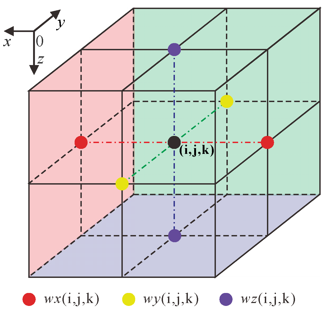
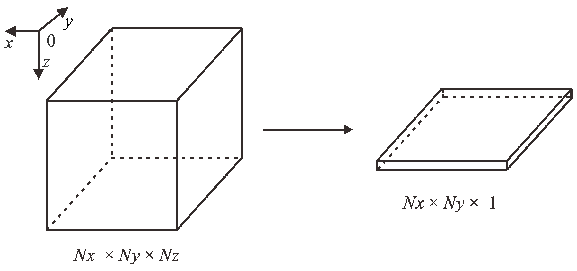
Each cube has three coefficients (wx, wy, and wz) that are positioned in the center of six surfaces (Figure 1). For each cube which belongs to an elliptical tube on the layer of xoy, wz is calculated by Equation (4). The calculation method of parameters a and b is given in the Section 2.2. If the original size of a 3D model is Nx × Ny × Nz, then each layer is defined as a Nx × Ny × 1 grid network (Figure 2). After this layer is divided into different elliptical tubes, the coefficient wz of all pore cubes composed of this layer can be calculated by Equation (4). The calculations of wx and wy are the same.
According to Equations (1), (3) and (4), a generalized Laplace equation in each cube can be expressed as:
where w represents the coefficient of one cube.
The finite initial pressures are set at the inlet and outlet faces via additional external grid-blocks facing the grid-blocks of porous media, and the Dirichlet boundary condition is applied there. No-flow boundary conditions are assumed on the other four faces, to which the Neumann’s boundary condition is applied. Because of null flow across grain boundaries, Neumann’s boundary condition at grain boundaries is also implemented here. The pressure is positioned in the center of each cube. Moreover, if the cubes with indices (i, j, k), (i − 1, j, k), (i + 1, j, k), (i, j − 1, k), (i, j + 1, k), (i, j, k − 1), and (i, j, k + 1) are pores, Equation (5) can be expressed by discretize equation. The central difference derivation at the cube with index (i, j, k) can be expressed as:
where, wx+ = (wx(i + 1,j,k) + wx(i,j,k))/2; wx− = (wx(i,j,k) + wx(I − 1,j,k))/2; wy+ = (wy(i,j + 1,k) + wy(i,j,k))/2; wy− = (wy(i,j,k) + wy(i,j − 1,k))/2; wz+ = (wy(i,j1,k + 1) + wz(i,j,k))/2; wz− = (wy(i,j,k) + wz(i,j,k − 1))/2 and the pressure values are the unknowns.
If the cubes adjacent to the cube with index (i, j, k) are grains, the form of Equation (6) will be changed. For only the cube with index (i − 1, j, k), which is a grain boundary in Equation (6), Equation (6) is expressed as:
Then, using central difference derivations for all cubes representing pores, Equation (5) can be expressed as:
where W represents the coefficient matrix, P represents an unknown column vector which is made up of the pressures of the center of the cubes (p1,1,1, p1,1,2, pNx,Ny,Nz), and B is the given column vector of boundary conditions (wz(1,1,1)PI, wz(1,2,1)PI,…,wz(Nx,Ny,Nz)PI, 0,…,0, wz(1,1,Nz)PO,…, wz(Nx,Ny,Nz)PO). We assume that the inlet and outlet surface pressures are constant and are represented by PI and PO, respectively (Figure 2). The fluid flows in direction z.
WP = B
As shown above, the matrix W is sparse, so the biconjugate stabilized method [45] is applied to calculate the pressure distribution. For large W, the biconjugate stabilized method can be memory efficient. By solving Equation (8), the spatial distribution of the pressure can be obtained and the total volume flow rate of the porous media in the macroscopic flow direction gives the following:
where, i and j are the horizontal and vertical coordinates on the cross section normal to the macroscopic flow direction, respectively, Jij is the mass flux of one cube on a one-cell thick layer normal to the macroscopic flow direction which pressure gradient has been applied, Aij is the cross-sectional area of one cube, and Δpij is the pressure drop between this cube and the adjacent cube in the macroscopic flow direction.
Then according to Darcy’s law, the effective permeability, K, of the porous media is:
where L represents the length of the porous media in the macroscopic flow direction, A represents the cross-sectional area of the porous media normal to the macroscopic flow direction, and PI and PO are the inlet and outlet pressures, respectively.
2.2. Elliptical Pore Approximation Method for the Calculation of Coefficient w
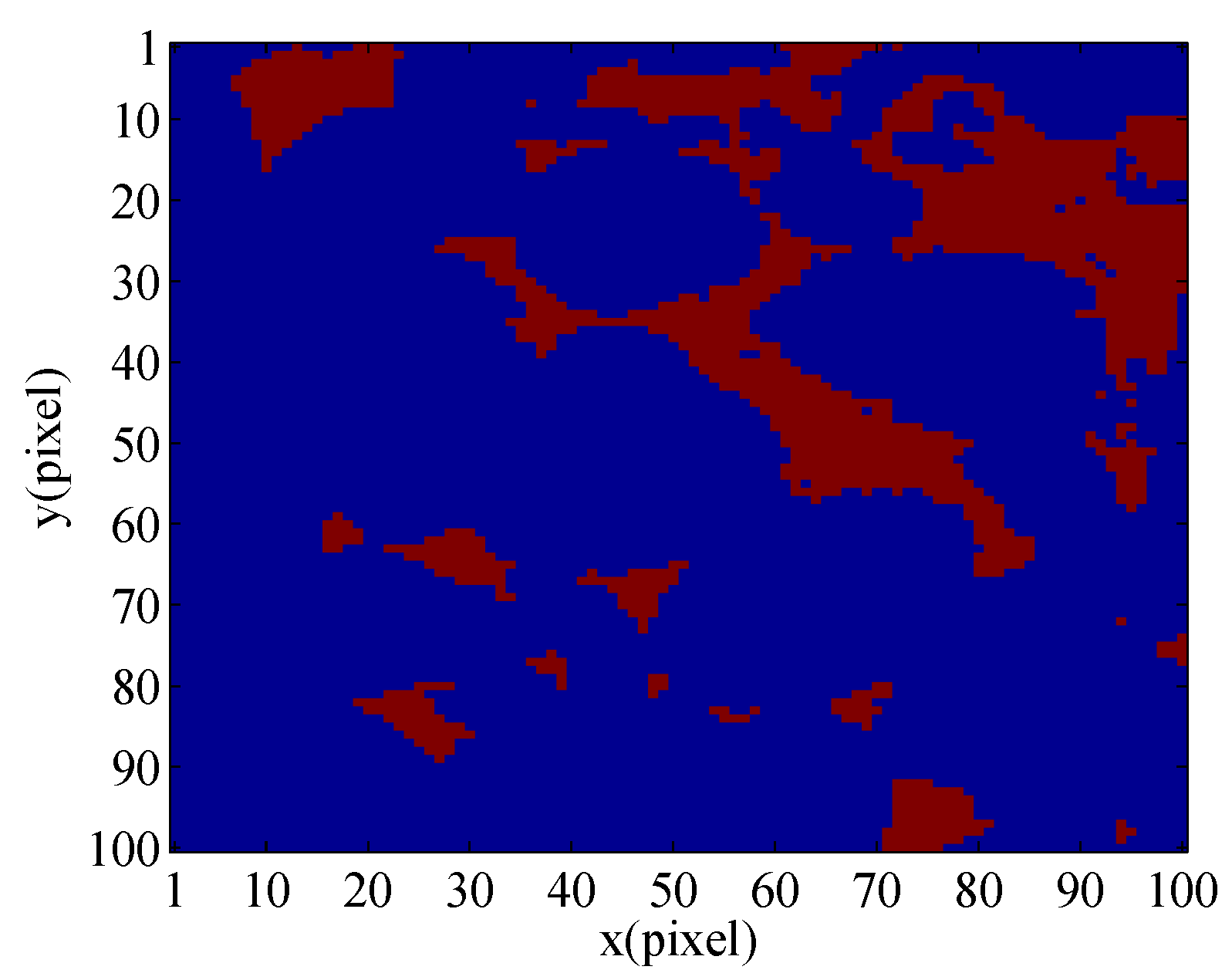
This section mainly introduces the calculation of the coefficients of all the cubes constructing the pore space in digital rock image. Here we partition each layer of the digital rock image into a series of interconnecting elliptical tubes [46]. Figure 3 shows that this layer of the digital rock is irregular. The red part is pore and the blue part is grain. For any elliptical tube that is perpendicular to the direction of z, all coefficients wz of the cubes inside this tube are of the same value which can be obtained by Equation (4).
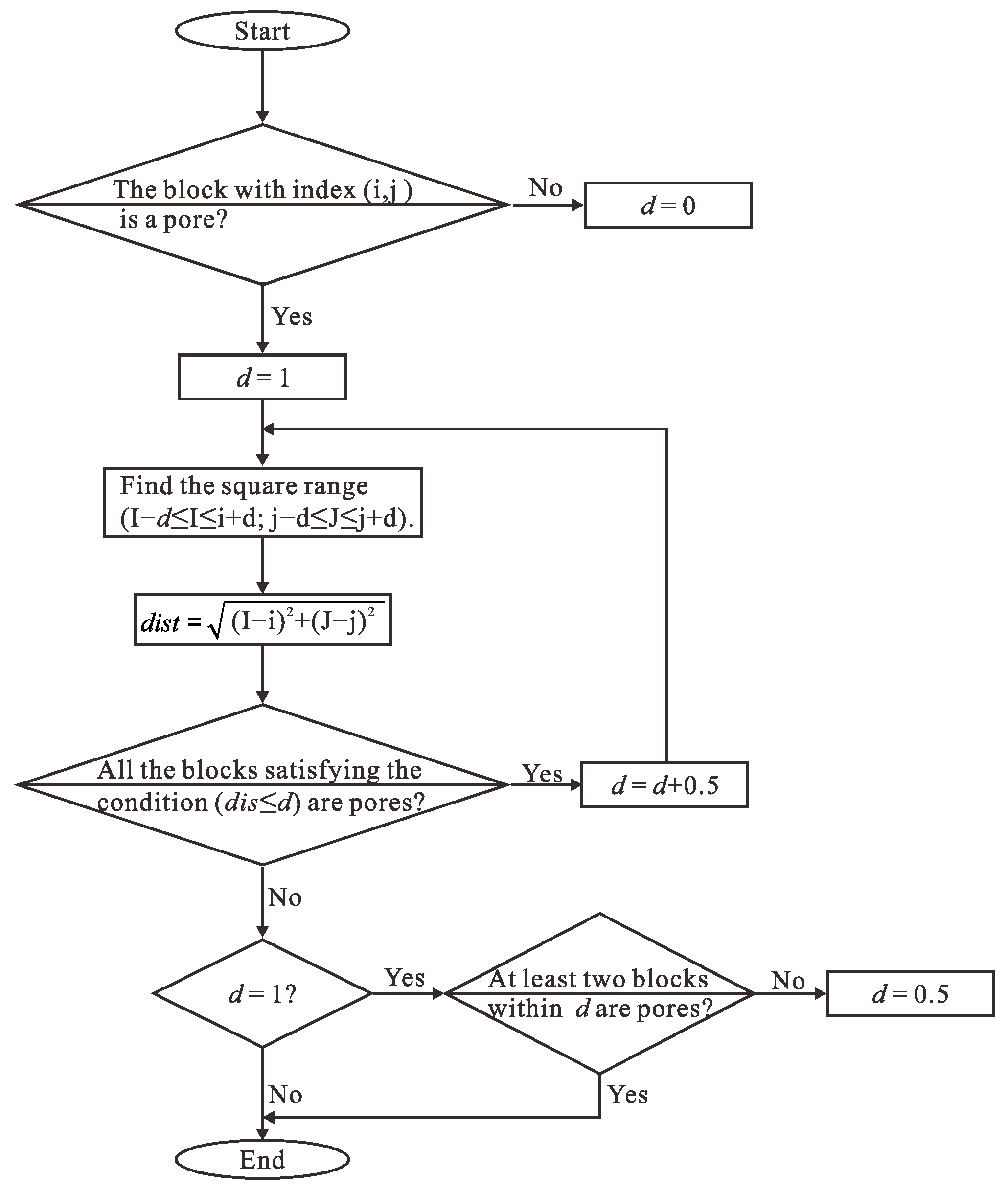
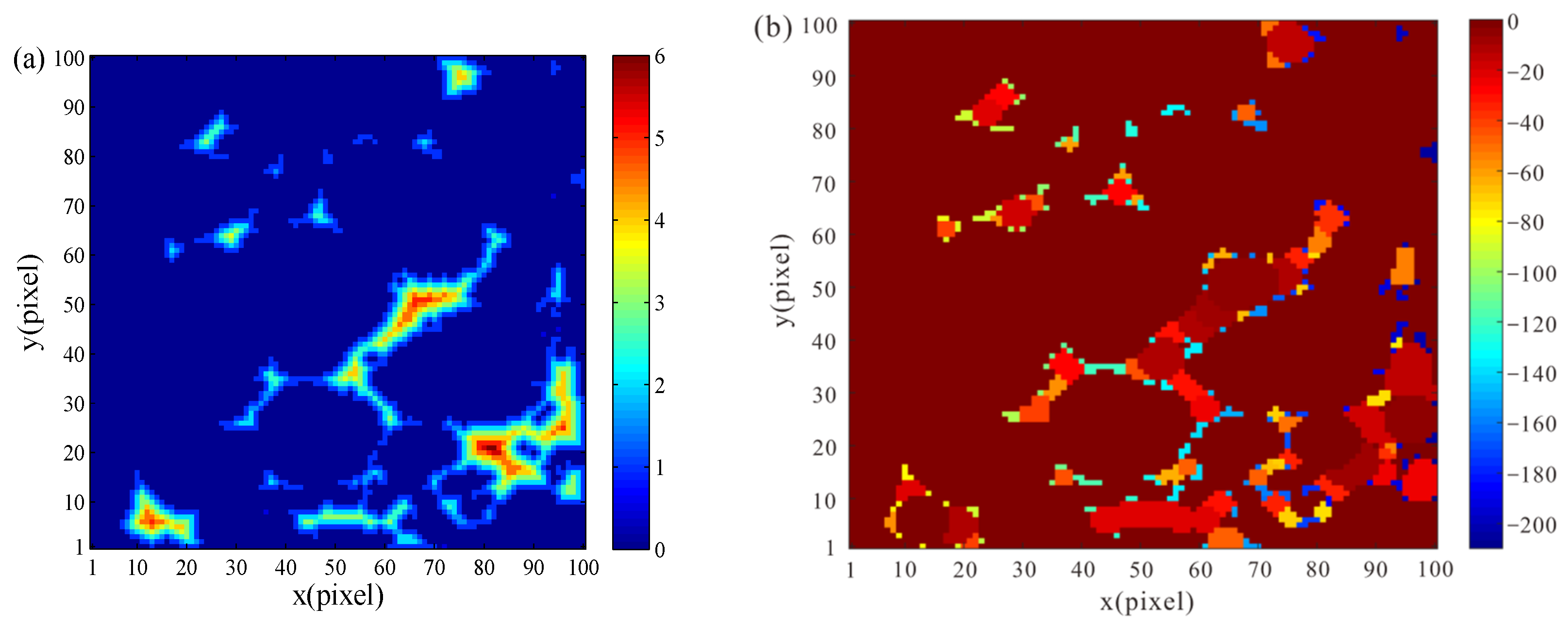
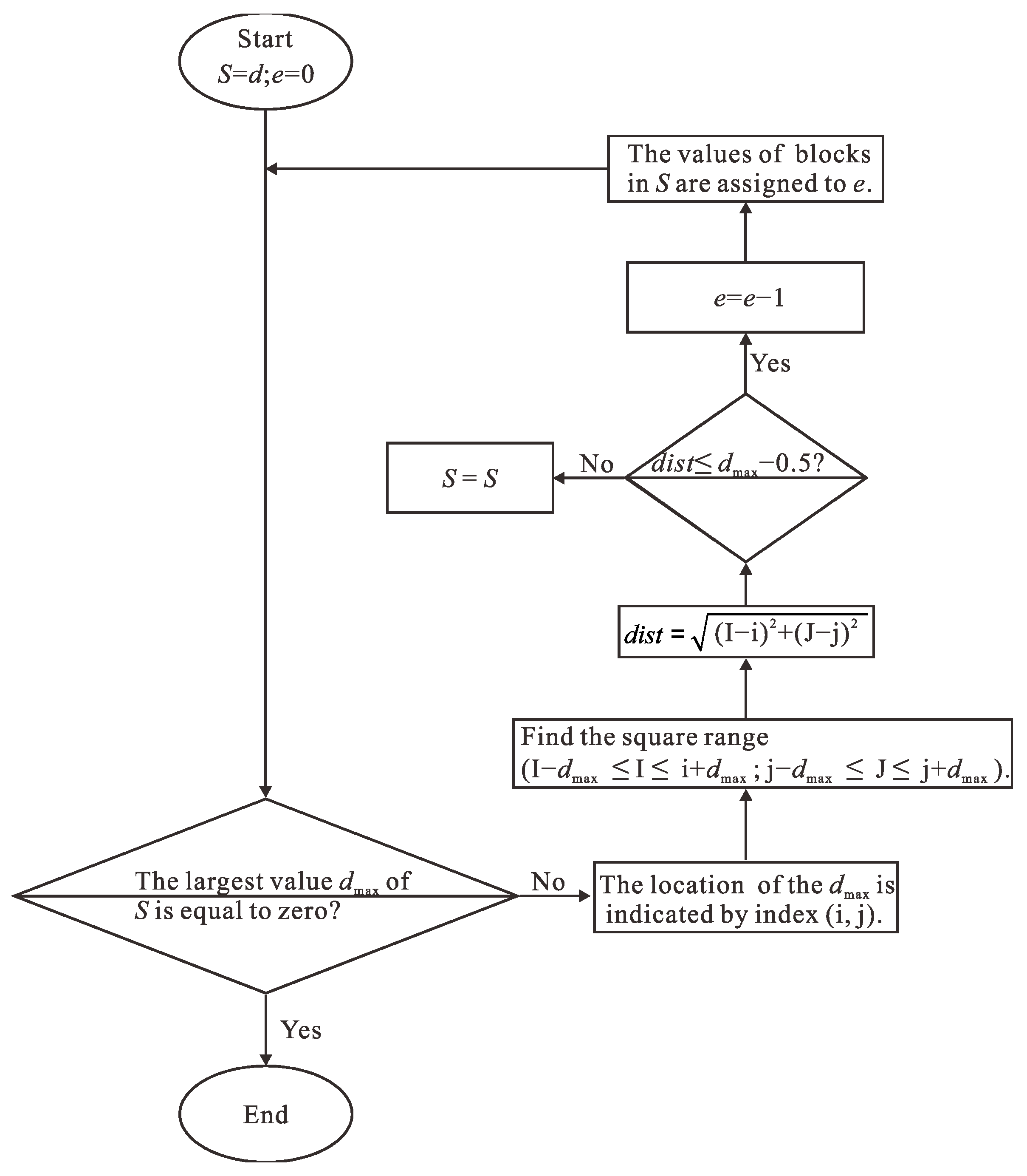
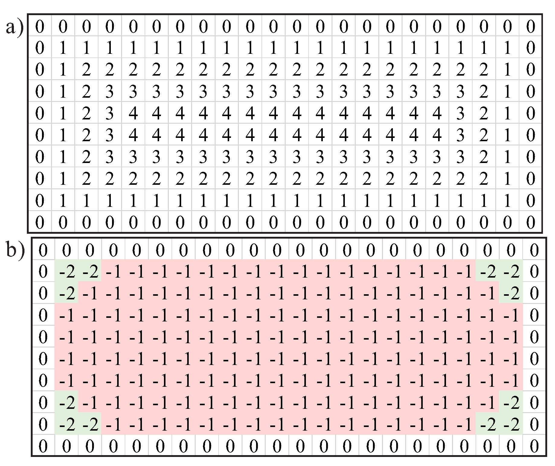
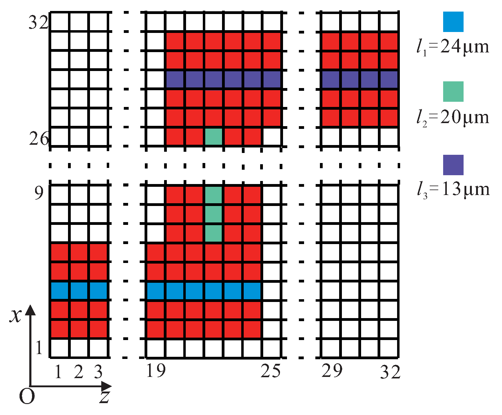
The definition of several key parameters is introduced here. rmax and r are the largest inscribed radius and the distance to the grain boundary, respectively; and dmax and d are the digital equivalents of rmax and r, respectively. As depicted in Figure 3, the size of a block is 1 pixel × 1 pixel. Firstly, we will introduce how to calculate the d of every block. For a block representing pore, its initial value of d is “1”. For a block representing grain, its initial value of d is “0”. For a certain block with index (i, j) constituting a pore, the square range is found (i − d ≤ I ≤ i + d; j − d ≤ J ≤ j + d). Then, the distances between the block with index (i, j) and all the blocks in the square range are calculated, indicated by dis. If all the blocks satisfying the condition (dis ≤ d) are pores, then the value of d becomes d + 0.5; if not, the value of d remains unchanged. Finally, if it is an isolated block, the d value of the block is reassigned to “0.5”. What’s more, we provide a flowchart of the algorithm to show the calculation process of d value more intuitively (Figure 4). Figure 5a shows the distribution of d for one layer of digital rock.
Next, we introduce the regional division of pores. Different regions are represented by S. d is assigned to S as the initial value. In this case, e represents the value of different regions and the initial value of e is “0”. The maximum value dmax of S is searched and the position of dmax is recorded at the first step. If the location of dmax is indicated by index (i, j), find the square range (i − dmax ≤ I ≤ i + dmax; j − dmax ≤ J ≤ j + dmax). Then, the distances between the block with index (i, j) and all the blocks in the square range are calculated, and are indicated by dist. The values of blocks satisfying the condition (dist ≤ (dmax − 0.5)) are assigned to (e − 1). Then the previous steps are repeated. S is finally determined until the maximum value of S is “0”. Different S values represent different regions at this time. Then each region is simulated by an ellipse and the coefficient w of every region can be calculated using Equation (4). Figure 6 shows the flowchart of the calculation of S. Figure 5b shows the distribution of S for one layer of digital rock.
3. Model Validation
In order to validate our method, we first apply IFDM to calculate four types of idealized porous media that have analytical or semi-empirical solutions [44,47,48,49,50]. Analytical permeability refers to the solution obtained by strict formula. Effective permeability refers to the solution obtained by numerical method. The four models are one of straight tubes with rectangular cross sections, a model consisting of two tube segments with circular cross sections in sequence, a model consisting of five tubes with circular cross sections, and a model consisting of three tubes with circular cross sections. The pore structure of the digital rock image is more complex than that of idealized porous media. Computation of the permeabilities for the 11 digital rock images from the Imperial College London by IFDM is given for further validation of the method [50]. The lithology of these digital rocks are carbonate rock, Berea sandstone and sandstone.
3.1. Model One: Straight Tubes with a Rectangular Cross Section
We first consider the simple case that the fluid flows through a straight tube with rectangular section, and the permeability of this model has an analytical solution. We compare the permeability calculated by IFDM with the analytical solution. For the straight tube with a rectangular section, the expression of velocity distribution can be expressed as [44]:
where u is the velocity, μ is the fluid viscosity, dp/dz is the pressure gradient in direction of z, and a and b represent the semi-major and semi-minor axes of the rectangular tube, respectively. x and y are the coordinates on the X and Y axes, respectively.
For the straight tube with a rectangular section, White (1991) provided an expression for calculating the volume flow rate of the tube [44]:
where 2a and 2b represent the length and width of the rectangle, respectively.
Combining Equation (12) with Darcy’s law, the analytical permeability of the straight tube can be expressed as:
where A is the cross-sectional area of the model normal to the main flow direction.
3.2. Model Two: Two Tube Segments with Circular Cross Sections in Sequence
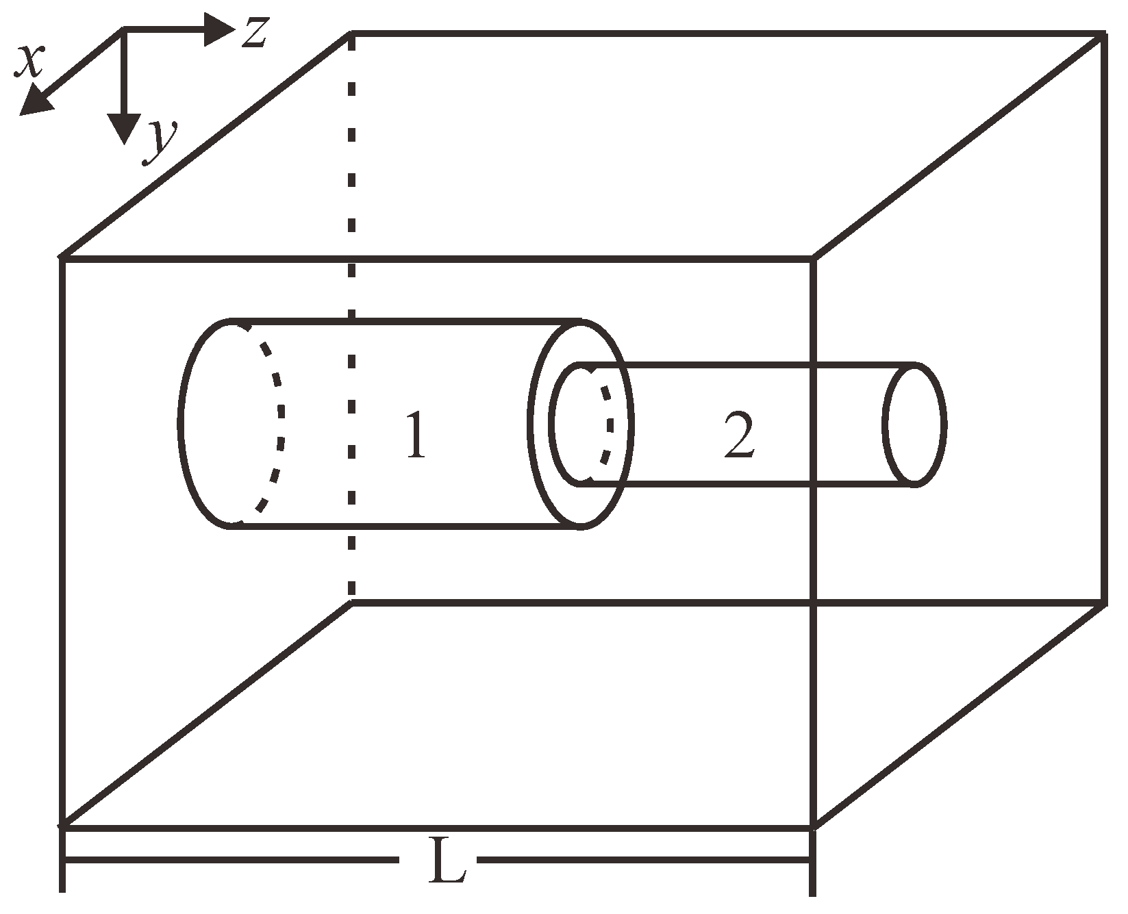
Figure 7 shows a model consisting of two tube segments in sequence [47]. The size of the model is L3. The flow direction is from left to right. The radii of the two segments are a1 and a2, respectively, and the length of both of the two segments are L/2. The volume flow rate of model two is [10,47]:
where Δh is applied piezometric head drop, constant ρ is the density of the single fluid, g is the gravitational acceleration.
3.3. Model Three: A Model Consisting of Five Tubes with Circular Cross Sections
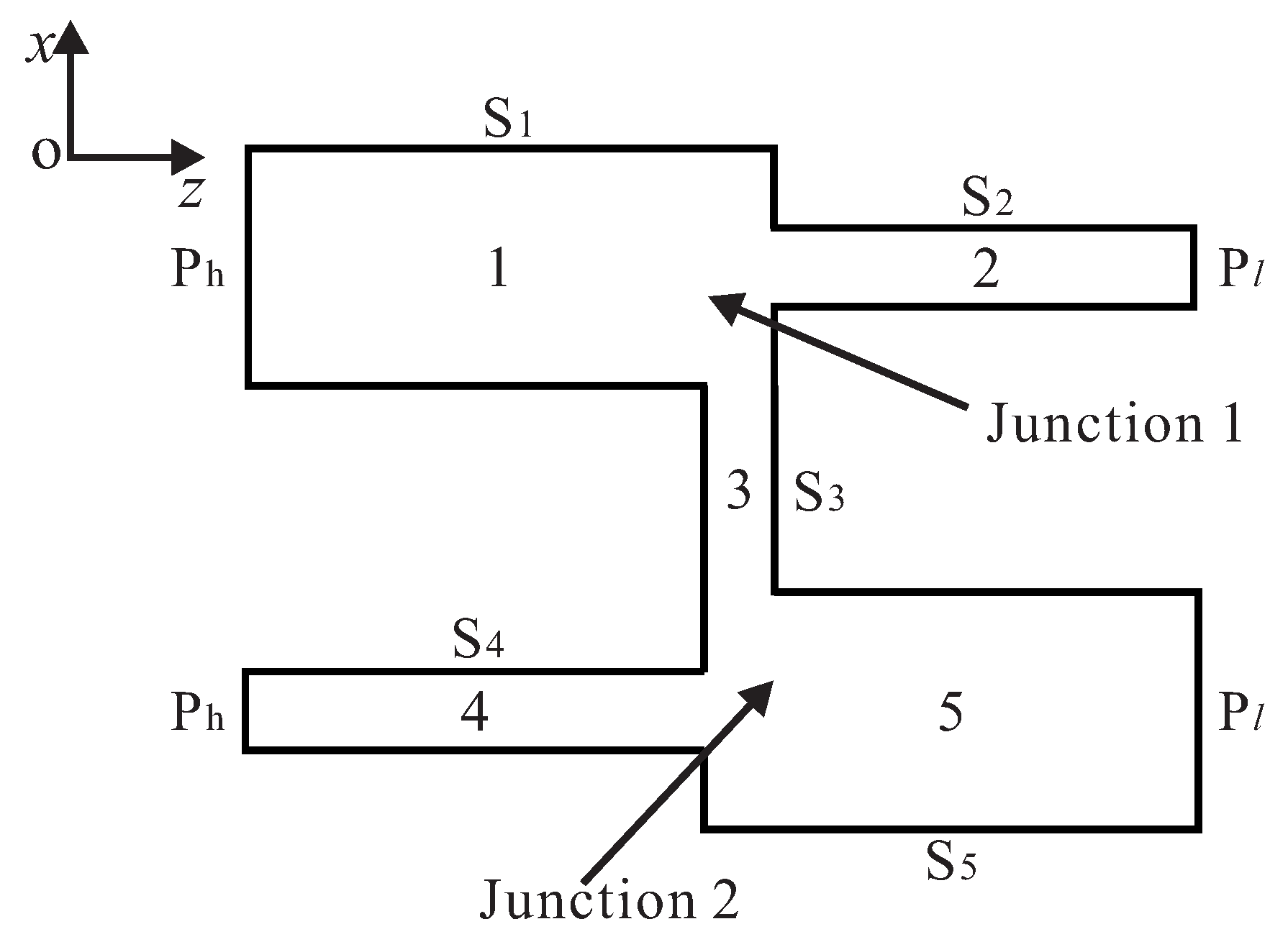
Figure 8 depicts the cross section of an idealized porous medium normal to the direction of y, which consists of five tubes. The flow direction is from left to right. The lengths of the tubes are denoted by S1, S2, S3, S4, and S5, respectively. The cross sections of all the tubes are circles. The diameters of tube 1 and 5 are δa. The diameters of tube 2 and 4 are δb and the diameter of tube 3 is δc. In order to apply IFDM to calculate the permeability of model three, this porous medium is divided into 64 × 64 × 64 μm blocks. The lengths of tubes 1, 2, 3, 4, and 5 are 30 μm, 29 μm, 30 μm, 24 μm, and 35 μm, respectively. The values of δa, δb, and δc are 15 μm, 11 μm, and 11 μm, respectively. This model is an idealized porous medium for understanding the flow phenomena, rather than for predicting permeabilities of real porous media. Ruth and Suman [48] analyzed the microscopic cross flow in idealized porous media and presented the “averaging theorem permeability”:
where k1 is the permeability of this model in one direction, fi represents the ratio of volumetric flow rate in tube i and the total volumetric flow rate, Si is the length of tube i, L is the length of the model in the main-flow direction (i = 1, 2, 3, 4, and 5). In , A is the cross-sectional area of the model normal to the main flow direction.
3.4. Model Four: A Model Consisting of Three Tubes with Circular Cross Sections
Kozeny [49] presented the well-known semi-empirical Kozeny-Carman equation and assumed that the porous medium could be regarded as a bunch of streamtubes. Carman [51] linked the microscopic fluid velocity to the Darcy velocity for porous media and introduced a tortuosity factor τ. The Kozeny-Carman equation is widely used in the calculation of the permeability of porous media. The effective permeability calculated by the Kozeny equation can be expressed as [52,53]:
where ϕ is the porosity, τ is the hydraulic tortuosity, Sr is the specific surface area per unit pore volume, f is the shape factor, and f = 2 for a tube with circular cross section.
3.5. The Permeability of Digital Rock Image
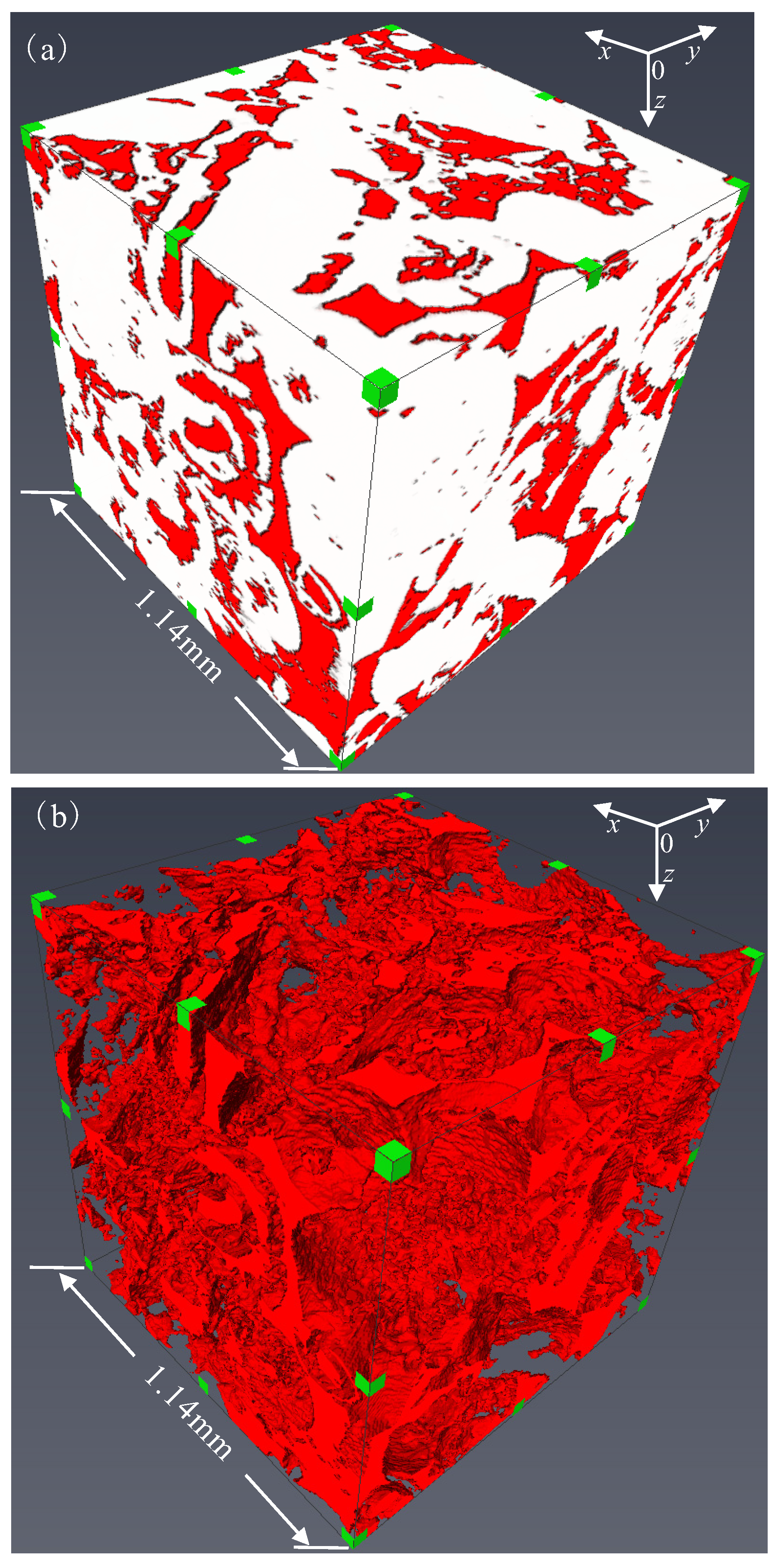
Figure 9 depicts the 3D micro CT image and pore space of carbonate C1, which indicates that the pore structure of the digital rock image is really very complex. Red is a pore space and white is a skeleton. Because of the complex pore structure in digital rock images, the IFDM is further confirmed by calculating the permeabilities of 11 digital rock images. Berea and Si (i = 1, 2, 3, …, 9) are sandstone. Isolated pores exist in digital rock images, which do not contribute to seepage, so we remove the isolated pores, which will save much computational time. 6-connected neighborhood is applied to classify the cubes representing the pores [54,55]. Assuming that there are only pores and solid skeleton in the digital rock model, the connected regions of pore pixels are detected by seed filling method [56]. A group of pixels connected with each other but not connected with other pixels are marked as a connected region, and then these connected regions are analyzed and classified. Seed filling algorithm is derived from computer graphics. The general steps are as follows:
- (1)
- Mark an unlabeled pixel as a seed. Mark the seed and create an empty stack;
- (2)
- All the neighboring pore pixels with a distance of 1 from the seed are retrieved. If the adjacent pore pixels are not marked, the adjacent pore pixels are incorporated into the stack;
- (3)
- Take out a pixel from the top of the stack as a new seed and repeat step (2);
- (4)
- Repeat steps (2) and (3) continuously until the stack is empty again.
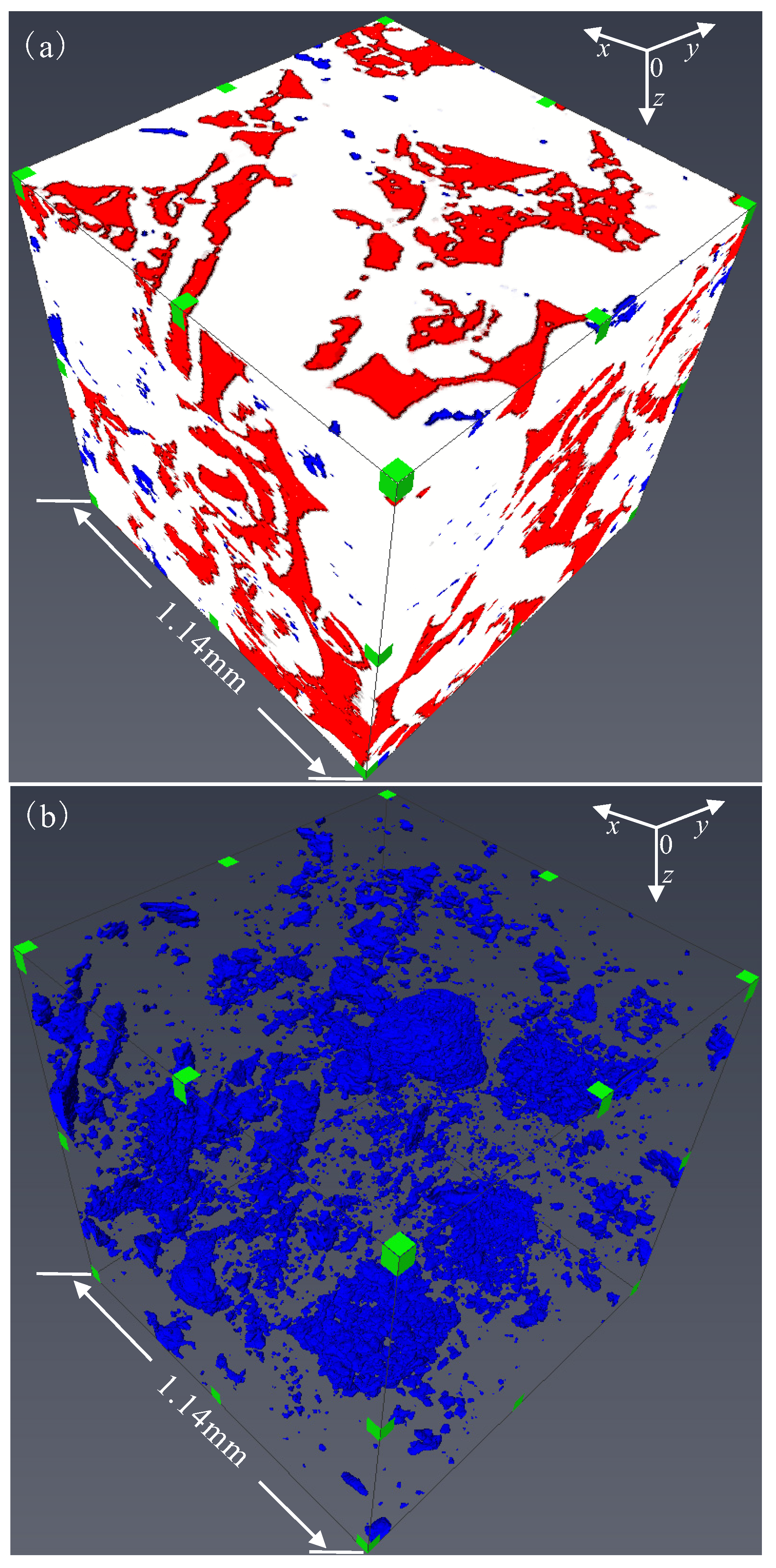
In the above steps, all the pixels and initial seeds that have been put on the stack are marked as a group. The connected pore space consists of all kinds of pores which connect the inlet and outlet faces. Here, C1 is taken as an example to show the effect of removing isolated pores. The red part shows the connected pores and the blue part shows the isolated pores in Figure 10a. Figure 10b shows the isolated pore space of C1.
4. Results and Discussion
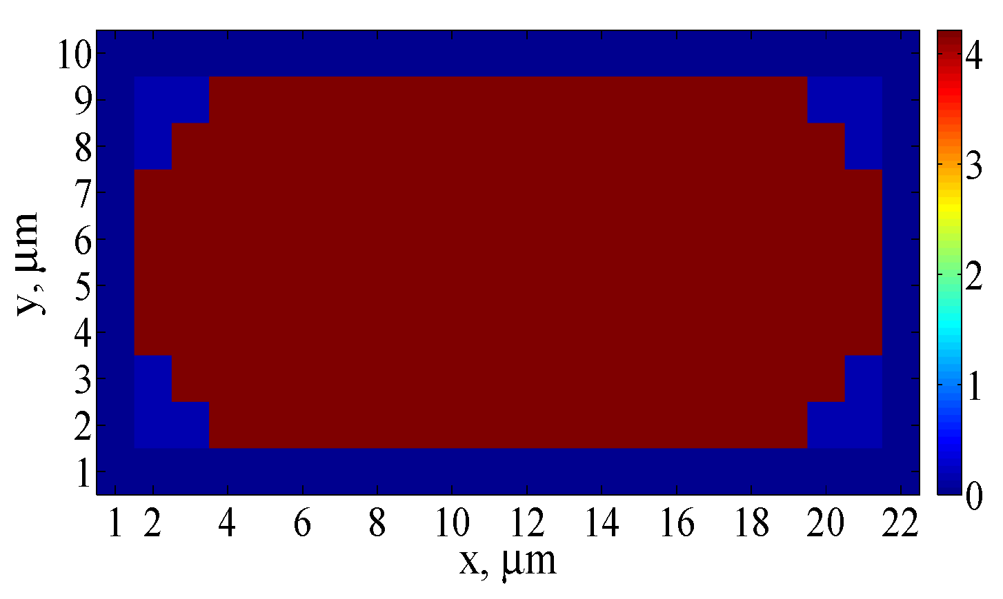
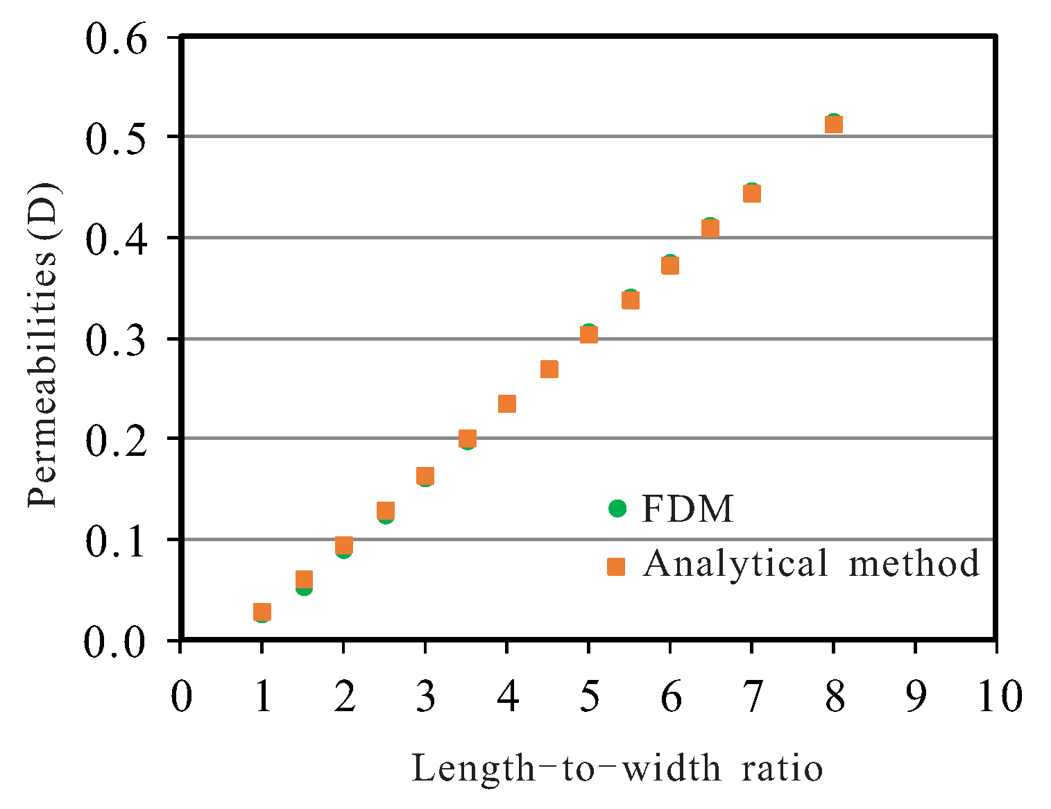
The model one is partitioned into 70 × 70 × 70 μm. We assume that the length and the width of the cross section are 20 μm and 8 μm, respectively. Figure 11a shows the distribution of d on the rectangular cross section and Figure 11b shows the partition of the rectangular cross section. Figure 12 depicts the distribution of w on this layer. And the distribution of w on each layer in three orthogonal directions can be calculated in the same way. Then the effective permeability of this model with a straight tube can be calculated by the IFDM. The permeability values of this straight tube calculated by IFDM and the analytical method are 0.126 D and 0.130 D, respectively. The estimated permeability presents an error of 3.1% in comparison with the analytical solution. Moreover, the permeabilities of straight tubes with different cross-sectional areas are calculated (Figure 13). The width of a cross section is constant and its value is 8 μm. The length-to-width ratio increases with increase of the length. The analytical solutions are in good agreement with the results calculated by IFDM. The IFDM presented in this study works well for this simple model. Moreover, Shabro et al. [27] presented a finite-difference approximation called FDGPA and the permeability of a 3D model with a straight tube was calculated by FDGPA. The size of the model is 400 μm × 400 μm × 400 μm and the rectangular cross section is 20 μm × 400 μm. The permeabilities calculated by analytical expression, FDGPA and the method presented in this study are 1.69 D, 0.8281 D and 1.62 D, respectively. The comparison results show that the method presented in this study has better applicability for elongated pores.
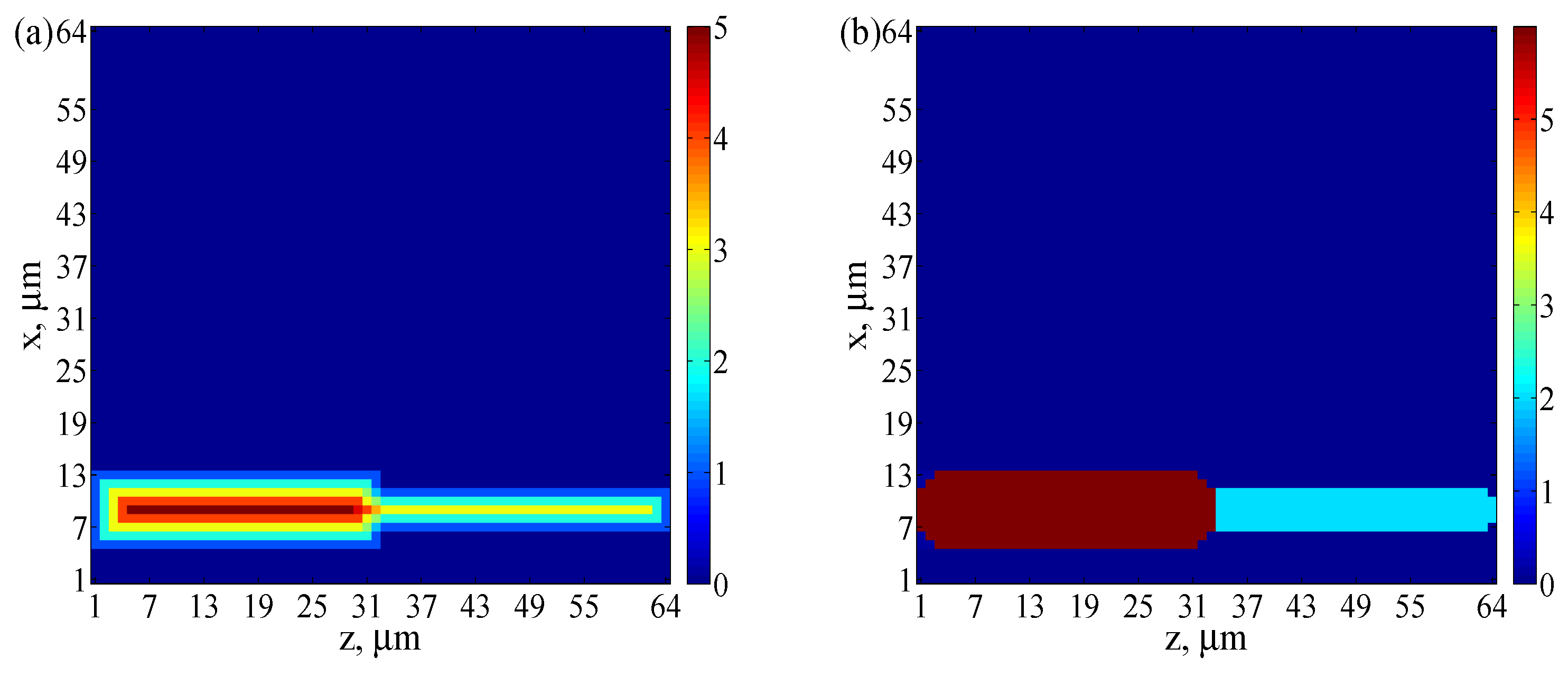
Model two is partitioned into 64 × 64 × 64 μm. Here, a1 and a2 are equal to 4.5 μm and 2.5 μm, respectively. We present the distributions of d and w for one layer as an example (Figure 14). After we get the distributions of d and w for all the layers in three orthogonal directions, we get the permeability of model two by IFDM. The permeabilities calculated by IFDM and analytical method are 0.0073 D and 0.0068 D, respectively. The error between these two results is 7.4%.
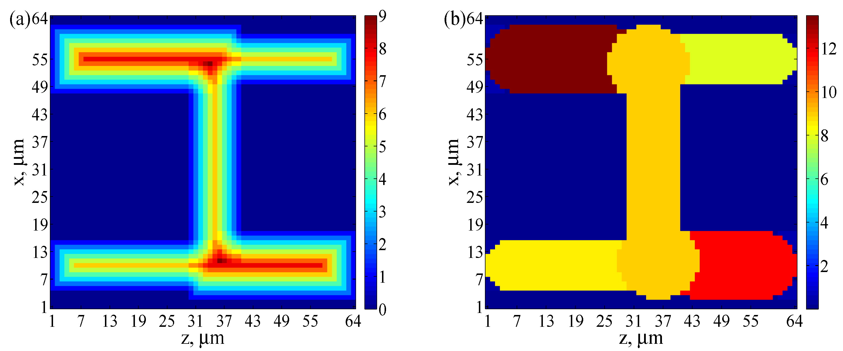
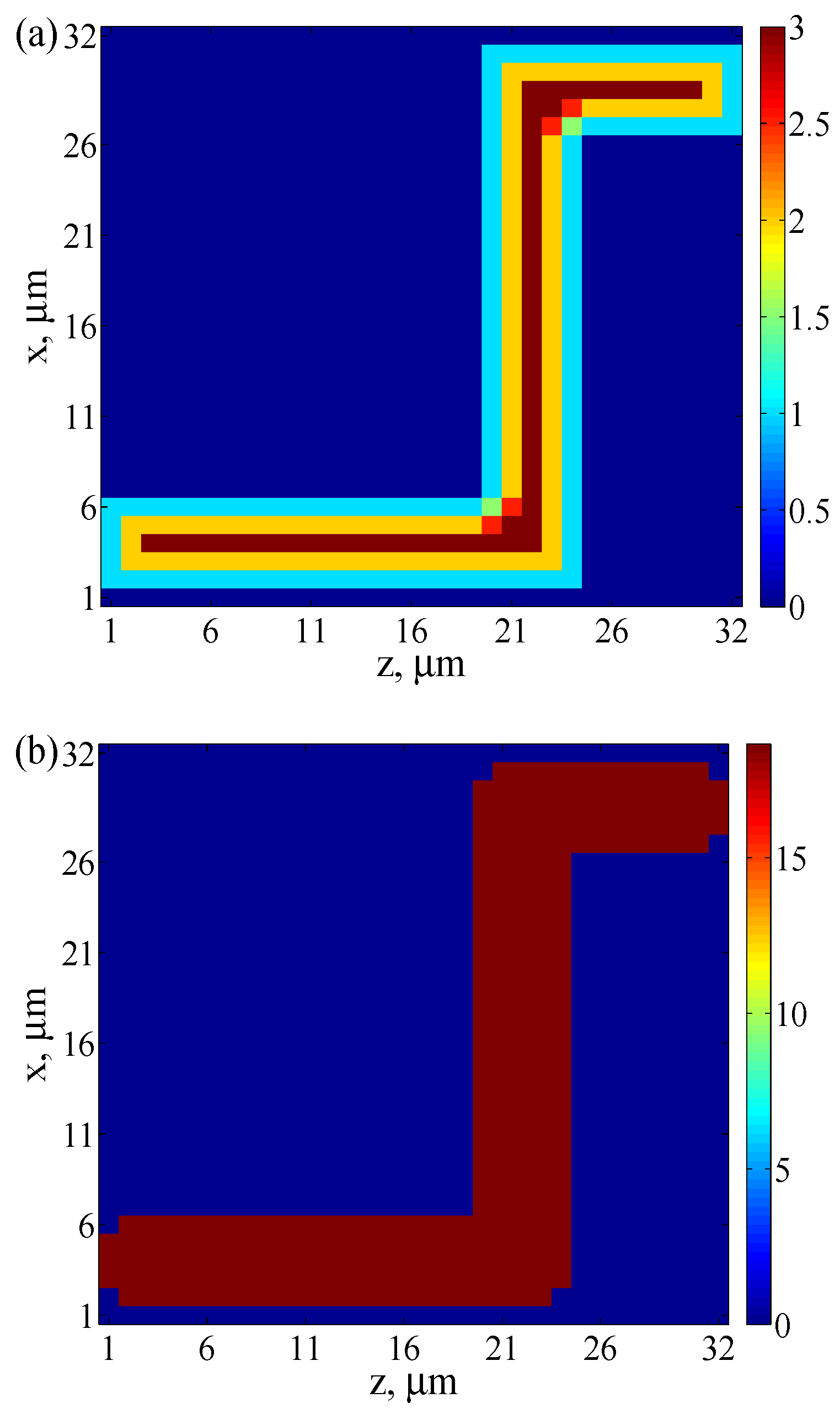
The effective permeability of model three can be calculated by IFDM. Figure 15a,b show the distribution of d and the distribution of coefficient w, respectively, for the cross section of Figure 8. The permeability values of this idealized porous medium calculated by IFDM and the averaging theorem method are 0.331 D and 0.342 D, respectively. The error between these two results is 3.2%.
Model four consists of three tubes with circular cross sections in sequence. All three tubes have the same diameters. The fluid flows from left to right. A layer of model four is illustrated in Figure 16. Then we can calculate the parameters in Equation (17). The porosity of model four is 0.0342. Here τ = (Le/L)2 represents the definition of the tortuosity. Le is the total length of the tube and L is the length of the model in the main flow direction. The hydraulic tortuosity is 2.743 and Sr is equal to 0.0273. Finally, we get the permeability of model four calculated by Equation (17) and the result is 0.0105 D. In addition, we present the distribution of d and w of the layer shown in Figure 16 as an example (Figure 17). When we calculate the distribution of coefficient w for all the layers in three orthogonal directions, the effective permeability of model four can be calculated by IFDM and the value is 0.0109 D. The error between the Kozeny equation and IFDM is 4%.
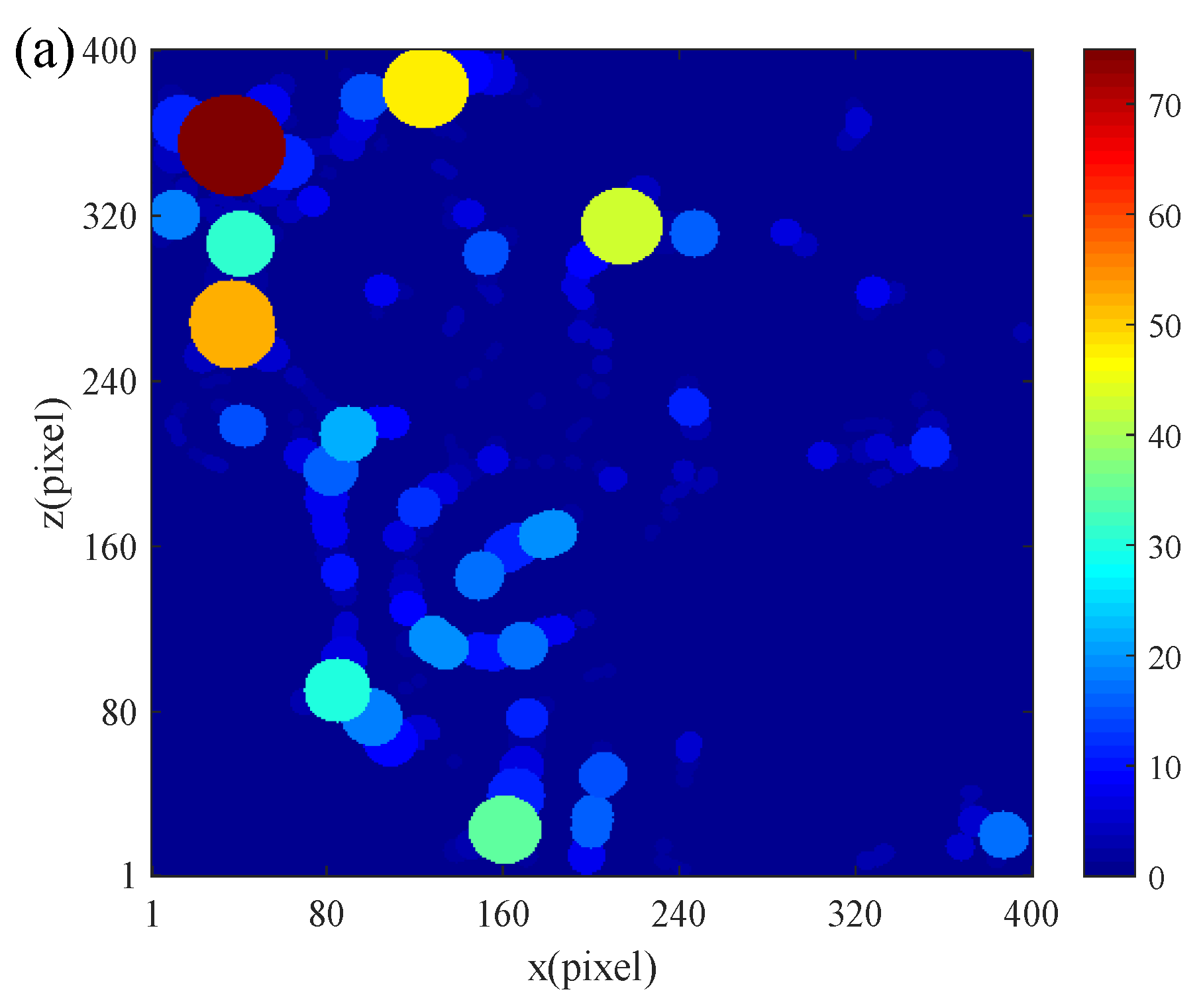
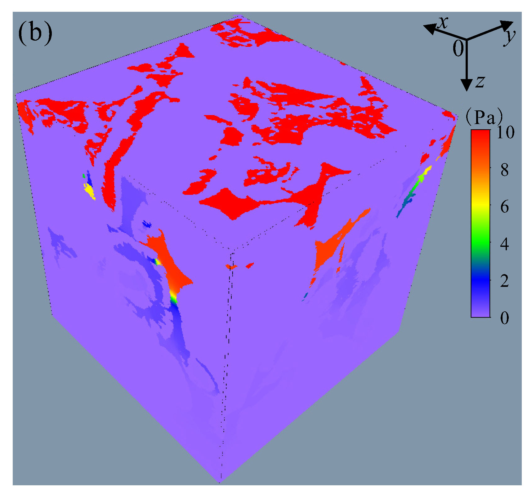
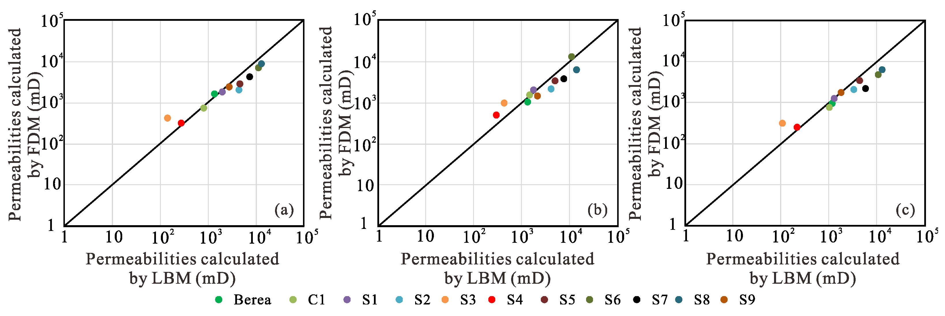
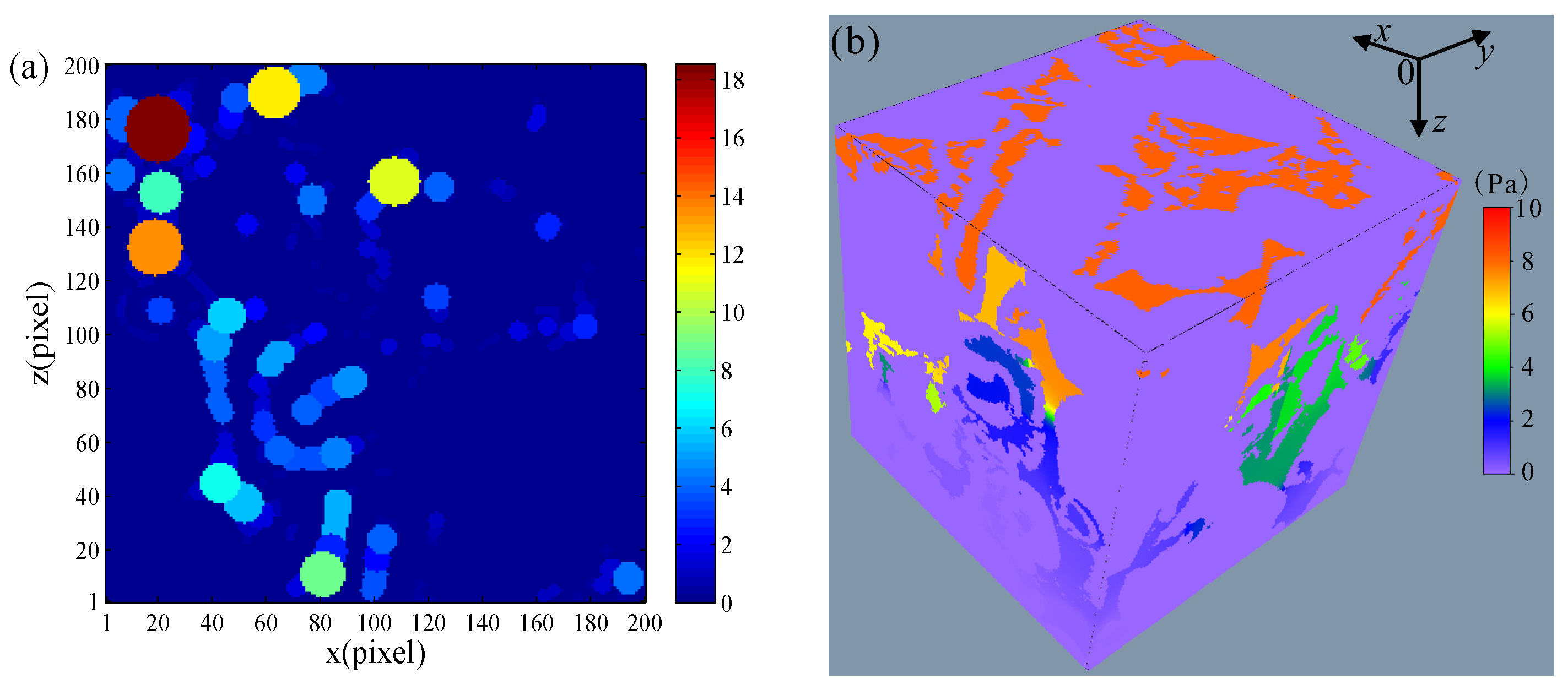
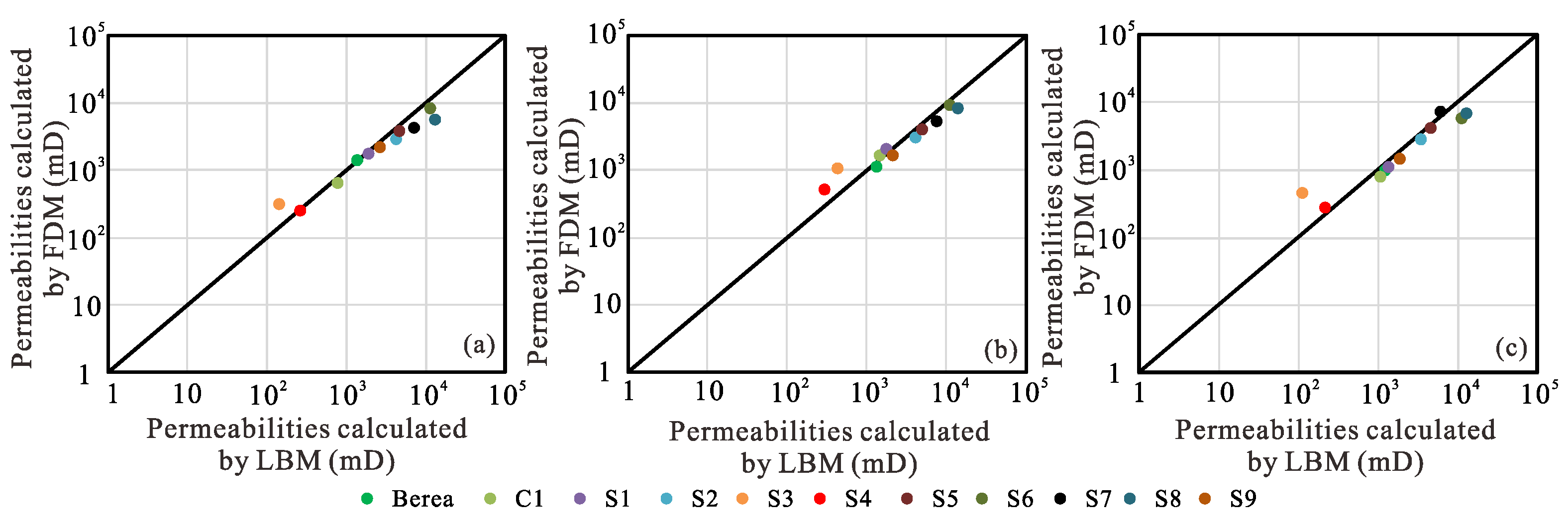
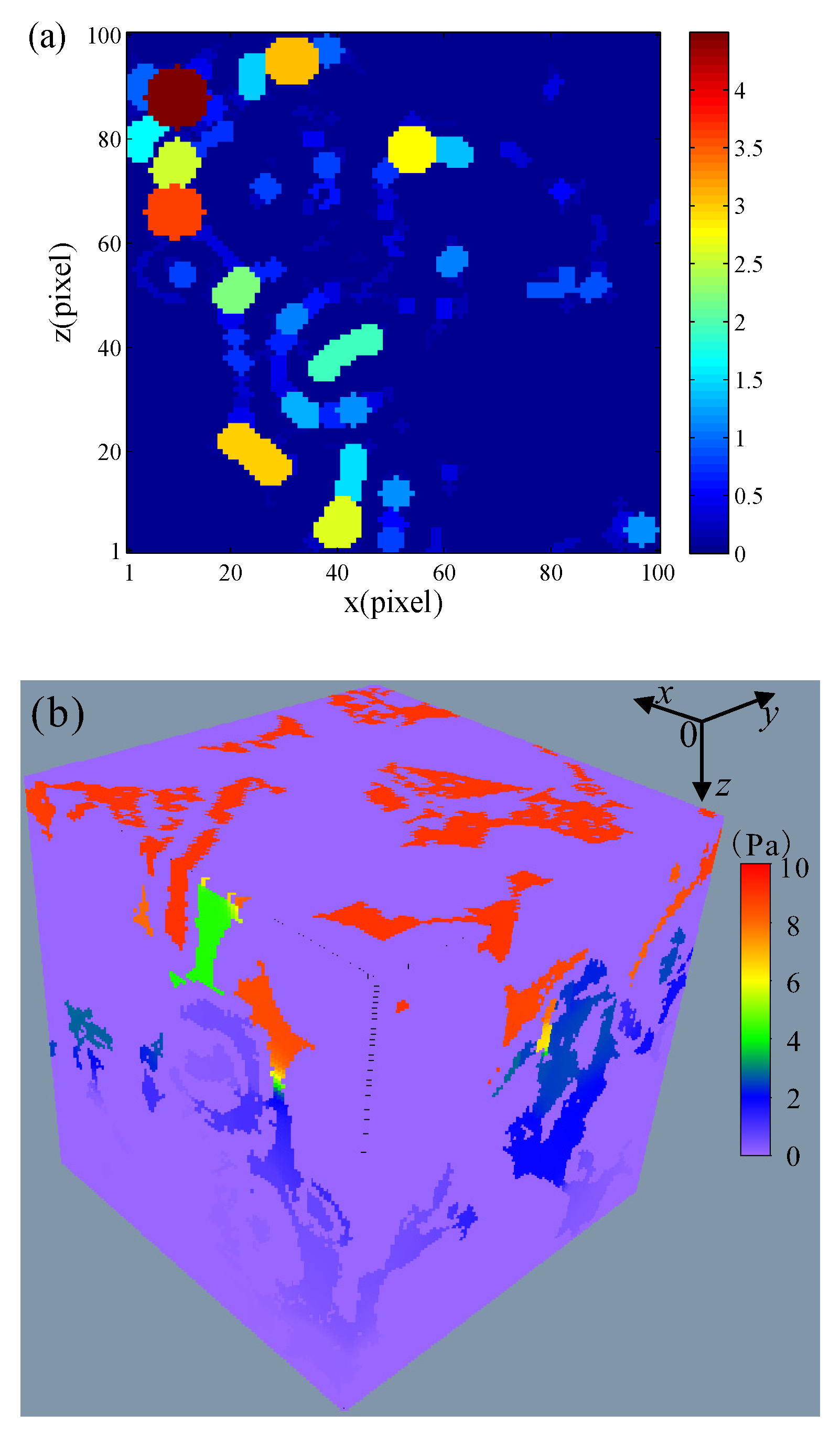
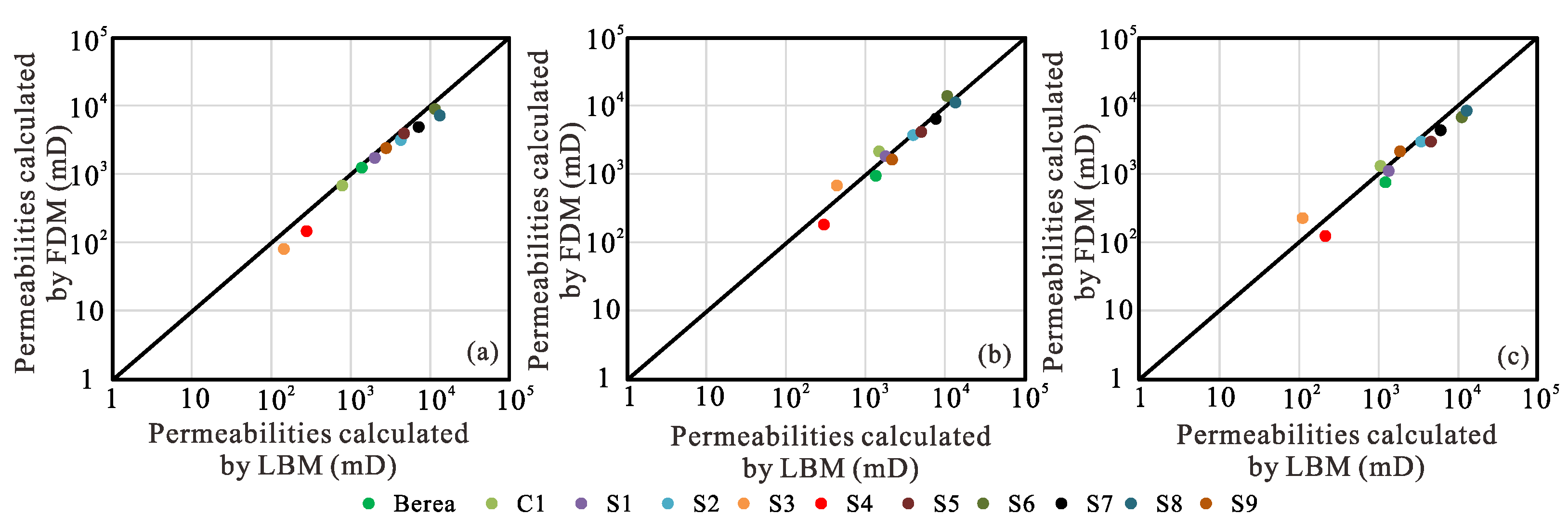
Table 1 shows the porosity, resolution and original size for these digital rock images. Berea sandstone and C1 carbonate digital rock images have 4003 voxels and the others have 3003 voxels. In order to verify the applicability of this method in digital cores, the effective permeabilities of original digital cores are calculated by IFDM. Figure 18 shows the distribution coefficients wy in one-cell layer of C1 and the pressure distribution of the whole digital rock. And we compared the permeabilities calculated by IFDM with the permeabilities calculated by LBM [50,57] in three orthogonal directions (Figure 19). This indicates that the predicted permeabilities calculated by IFDM usually agree with the permeabilities calculated by LBM. If we calculate the permeabilities of digital rock images at their original size by IFDM, it will take a great deal of time and computer memory. Consequently, we need to coarsen the grid while ensuring the accuracy of the calculation of permeability. When grids are coarsened, the calculation results will become inaccurate for the traditional finite difference method [27]. Sometimes it is even necessary to refine the grid to obtain more accurate values. When the size of digital core is large, the traditional finite difference method is obviously no longer applicable. Next, we will introduce whether the finite difference method proposed in this study can get reasonable results in the case of grid coarsening. A grid coarsened two times is acceptable for calculation of permeability with good accuracy [20]. Therefore, we first calculated the effective permeabilities of 11 digital rock images after coarsening the grid two times. And C1 carbonate digital rock is taken as an example to illustrate the specific permeability calculation process. Constant pressures are applied to two surfaces perpendicular to direction of z. Firstly, we use the elliptical pore approximation method to obtain the coefficients distribution of all grids. Figure 20a shows the distribution coefficients wy in one-cell layer of C1. Secondly, the pressure distribution of the whole digital rock is obtained by solving the Laplace equations (Figure 20b). Finally, the effective permeability of digital rock is obtained by Equations (9) and (10) in direction of z. We compare the results calculated by finite difference method with the absolute permeabilities calculated by LBM (Figure 21), which shows that the permeability calculation method proposed in this study is feasible for digital rock images. However, the size of the digital rock images used in this study is still too large after coarsening the grid two times. In this study, we calculated the permeabilities of the digital rock images after grid coarsening four times for Berea sandstone and C1 carbonate, and three times for the other digital rock images. Figure 22 shows the distribution coefficients wy in one-cell layer of C1 and the pressure distribution of the whole digital rock. The size of all the digital rock images was made 1003 when we compared the permeabilities calculated by IFDM with the permeabilities calculated by LBM [50,57] in three orthogonal directions (Figure 23). This indicates that the predicted permeabilities calculated by IFDM usually agree with the permeabilities calculated by LBM. Figure 21 and Figure 23 show that the results calculated by FDM and LBM are not exactly the same. This discrepancy is suggested to be related to a combination of image resolution and discretization effects [5]. In summary, the IFDM performs well for digital rock images even after grid coarsening.
5. Conclusions
We introduced an IFDM to model the flow of fluids at pore scale and calculate the permeabilities of porous media and digital rock images. What’s more, this study reveals that the elliptical pore approximation method works well for the calculation of the coefficient w of irregular cross sections. The IFDM shows good performance for the permeability estimation of a discrete model. The technique is more amenable for calculating the permeabilities of model one and model two, compared with the analytical solution. The permeability calculated by IFDM is compared with the averaging theorem permeability for model three and the permeability calculated by IFDM is compared with the semi-empirical Kozeny equation for model four. The error in all comparisons is below 10%. Moreover, we also demonstrate the validity of the IFDM by comparing its results with those of LBM for digital rock images. In order to improve the efficiency of the IFDM, grid coarsening is necessary. Grid coarsening of two, three or four times is acceptable, and the permeability calculated by the IFDM agrees well with the LBM result.
Author Contributions
Methodology, S.W., K.W. and H.Z.; software, J.W., W.H. and L.N.; Writing—original draft preparation, S.W.; Writing—review and editing, K.W., J.Z., J.W., W.H. and L.N.; Investigation, K.W., H.Z. and J.Z. All authors have read and agreed to the published version of the manuscript.
Funding
This research was funded by Shandong Provincial Natural Science Foundation of China, grant number ZR2020QE136.
Institutional Review Board Statement
Not applicable.
Informed Consent Statement
Not applicable.
Data Availability Statement
All processed data generated or used during the study appear in the submitted article. Raw data may be provided on reasonable request from the corresponding author.
Acknowledgments
Special thanks go to Martin Blunt and his research group at Imperial College London for providing the pore-scale micro-CT-image.
Conflicts of Interest
The authors declare no conflict of interest. The funders had no role in the design of the study; in the collection, analyses, or interpretation of data; in the writing of the manuscript, or in the decision to publish the results.
Nomenclature
| a | Semi-major axis of the elliptical tube |
| Aij | Cross-sectional area of one cube |
| B | Given column vector of boundary conditions |
| b | Semi-minor axis of the elliptical tube |
| C1 | Carbonate digital rock |
| CT | Computed tomography |
| D | Darcy |
| d | Digital equivalent of r |
| dmax | Digital equivalent of rmax |
| dp/dz | Pressure gradient in direction of z |
| f | Shape factor |
| FDM | Finite difference method |
| fi | Ratio of volumetric flow rate in tube i |
| g | The gravitational acceleration |
| i | Horizontal coordinate on the cross section normal to the macroscopic flow direction |
| IFDM | Improved finite difference method |
| Jij | Mass flux of one cube on a one-cell thick layer normal to the macroscopic flow direction |
| J | Mass flux |
| j | Vertical coordinate on the cross section normal to the macroscopic flow direction |
| K | Effective permeability |
| kkc | Effective permeability calculated by the Kozeny equation |
| Krectangular | Analytical permeability of the straight tube |
| k1 | Permeability of this model in one direction |
| L | Length of the porous media in the macroscopic flow direction |
| Le | The total length of the tube in model four |
| LBM | Lattice-Boltzmann method |
| Nx | The number of pixels in the direction of x |
| Ny | The number of pixels in the direction of y |
| Nz | The number of pixels in the direction of z |
| Qtot | Total volume flow rate of the porous media in the macroscopic flow direction PO: outlet pressure |
| p | The pressure in the model |
| P | Unknown column vector consisting of the pressures of the center of the cubes |
| PI | Inlet pressure |
| FDGPA | Finite-difference geometrical pore approximation |
| Q | Volume flow rate |
| rmax | Largest inscribed radius |
| r | Distance to the pore wall |
| S | The number of different regions |
| Si | Length of tube i |
| Sr | Specific surface area per unit pore volume |
| W | Coefficient matrix |
| 3D | Three dimensional |
| μ | Fluid viscosity |
| ρ | Fluid density |
| wx | Coefficient in direction of x |
| wy | Coefficient in direction of yd |
| wz | Coefficient in direction of z |
| w | Coefficient of one cube |
| Δpij | Pressure drop between this cube and the adjacent cube in the macroscopic flow direction |
| ϕ | Porosity |
| τ | Hydraulic tortuosity |
| δa | The diameters of tube 1 and 5 in model three |
| δb | The diameters of tube 2 and 4 in model three |
| δc | The diameters of tube 3 in model three |
| Δη | Applied piezometric head drop |
References
- Mostaghimi, P.; Blunt, M.J.; Bijeljic, B. Computations of absolute permeability on micro-CT images. Math. Geosci. 2013, 45, 103–125. [Google Scholar] [CrossRef]
- Esterhuizen, G.; Karacan, C. A methodology for determining gob permeability distributions and its application to reservoir modeling of coal mine longwalls. In Proceedings of the SME Annual Meeting, Denver, CO, USA, 25–28 February 2007. [Google Scholar]
- Tutak, M.; Brodny, J. The impact of the strength of roof rocks on the extent of the zone with a high risk of spontaneous coal combustion for fully powered longwalls ventilated with the y-type system—A case study. Appl. Sci. 2019, 9, 5315. [Google Scholar] [CrossRef] [Green Version]
- Arns, C.H.; Knackstedt, M.A.; Pinczewski, M.V.; Lindquist, W.B. Accurate estimation of transport properties from microtomographic images. Geophys. Res. Lett. 2001, 28, 3361–3364. [Google Scholar] [CrossRef]
- Arns, C.H.; Knackstedt, M.A.; Pinczewski, W.V.; Martys, N.S. Virtual permeametry on microtomographic images. J. Pet. Sci. Eng. 2004, 45, 41–46. [Google Scholar] [CrossRef]
- Arns, C.H.; Bauget, F.; Limaye, A.; Sakellariou, A.; Senden, T.; Sheppard, A.; Sok, R.M.; Pinczewski, V.; Bakke, S.; Berge, L.I. Pore scale characterization of carbonates using X-ray microtomography. SPE J. 2005, 10, 475–484. [Google Scholar] [CrossRef]
- Keehm, Y.; Mukerji, T.; Nur, A. Permeability prediction from thin sections: 3D reconstruction and Lattice-Boltzmann flow simulation. Geophys. Res. Lett. 2004, 31, L04606. [Google Scholar] [CrossRef]
- Knackstedt, M.A.; Latham, S.; Madadi, M.; Sheppard, A.; Varslot, T.; Arns, C. Digital rock physics: 3D imaging of core material and correlations to acoustic and flow properties. Lead. Edge 2009, 28, 28–33. [Google Scholar] [CrossRef]
- Zhao, J.; Sun, J.; Liu, X.; Chen, H.; Cui, L. Numerical simulation of the electrical properties of fractured rock based on digital rock technology. J. Geophys. Eng. 2013, 10, 055009. [Google Scholar] [CrossRef]
- Orlov, D.; Ebadi, M.; Muravleva, E.; Volkhonskiy, D.; Koroteev, D. Different Methods of Permeability Calculation in Digital Twins of Tight Sandstones. J. Nat. Gas Sci. Eng. 2021, 87, 103750. [Google Scholar] [CrossRef]
- Cai, J.; Sun, S.; Habibi, A.; Zhang, Z. Emerging Advances in Petrophysics: Porous Media Characterization and Modeling of Multiphase Flow. Energies 2019, 12, 282. [Google Scholar] [CrossRef] [Green Version]
- Tryggvason, G.; Bunner, B.; Esmaeeli, A.; Juric, D.; Al-Rawahi, N.; Tauber, W.; Han, J.; Nas, S.; Jan, Y.-J. A front-tracking method for the computations of multiphase flow. J. Comput. Phys. 2001, 169, 708–759. [Google Scholar] [CrossRef] [Green Version]
- Blunt, M.J. Flow in porous media—Pore-network models and multiphase flow. Curr. Opin. Colloid Interface Sci. 2001, 6, 197–207. [Google Scholar] [CrossRef]
- Parker, J.; Lenhard, R.; Kuppusamy, T. A parametric model for constitutive properties governing multiphase flow in porous media. Water Resour. Res. 1987, 23, 618–624. [Google Scholar] [CrossRef]
- Gao, Z.; Dang, W.; Mu, C.; Yang, Y.; Li, S.; Grebogi, C. A novel multiplex network-based sensor information fusion model and its application to industrial multiphase flow system. IEEE Trans. Ind. Inform. 2018, 14, 3982–3988. [Google Scholar] [CrossRef] [Green Version]
- Saxena, N.; Alpak, F.O.; Hows, A.; Freeman, J.; Hofmann, R.; Appel, M. Estimating Fluid Saturations from Capillary Pressure and Relative Permeability Simulations Using Digital Rock. Transp. Porous Media 2021, 136, 863–878. [Google Scholar] [CrossRef]
- Guo, Z.; Zhao, T. Lattice Boltzmann model for incompressible flows through porous media. Phys. Rev. E 2002, 66, 036304. [Google Scholar] [CrossRef]
- Wang, J.; Chen, L.; Kang, Q.; Rahman, S.S. The lattice Boltzmann method for isothermal micro-gaseous flow and its application in shale gas flow: A review. Int. J. Heat Mass Transf. 2016, 95, 94–108. [Google Scholar] [CrossRef] [Green Version]
- He, X.; Luo, L.-S. Lattice Boltzmann model for the incompressible Navier–Stokes equation. J. Stat. Phys. 1997, 88, 927–944. [Google Scholar] [CrossRef]
- Zakirov, T.; Galeev, A. Absolute permeability calculations in micro-computed tomography models of sandstones by Navier-Stokes and lattice Boltzmann equations. Int. J. Heat Mass Transf. 2019, 129, 415–426. [Google Scholar] [CrossRef]
- Yang, L.; Yang, J.; Boek, E.; Sakai, M.; Pain, C. Image-based simulations of absolute permeability with massively parallel pseudo-compressible stabilised finite element solver. Comput. Geosci. 2019, 23, 881–893. [Google Scholar] [CrossRef]
- Zhang, H.; Yin, X.; Zong, Z. Rock moduli estimation of inhomogeneous two-phase media with finite difference modeling algorithm. J. Geophys. Eng. 2018, 15, 1517–1527. [Google Scholar]
- Alpak, F.; Samardžić, A.; Frank, F. A distributed parallel direct simulator for pore-scale two-phase flow on digital rock images using a finite difference implementation of the phase-field method. J. Pet. Sci. Eng. 2018, 166, 806–824. [Google Scholar] [CrossRef]
- Osorno, M.; Uribe, D.; Ruiz, O.E.; Steeb, H. Finite difference calculations of permeability in large domains in a wide porosity range. Arch. Appl. Mech. 2015, 85, 1043–1054. [Google Scholar] [CrossRef] [Green Version]
- Igboekwe, M.U.; Achi, N.J. Finite difference method of modelling groundwater flow. J. Water Resour. Prot. 2011, 3, 192–198. [Google Scholar] [CrossRef] [Green Version]
- Narasimhan, T.N.; Witherspoon, P.A. An integrated finite difference method for analyzing fluid flow in porous media. Water Resour. Res. 1976, 12, 57–64. [Google Scholar] [CrossRef] [Green Version]
- Shabro, V.; Torres-Verdín, C.; Javadpour, F.; Sepehrnoori, K. Finite-difference approximation for fluid-flow simulation and calculation of permeability in porous media. Transp. Porous Media 2012, 94, 775–793. [Google Scholar] [CrossRef]
- Jqa, B.; Mma, B.; Haab, C. An investigation on the robustness and accuracy of permeability estimation from 3D μ-CT images of rock samples based on the solution of Laplace‘s equation for pressure. Comput. Geosci. 2021, 155, 104857. [Google Scholar]
- Manwart, C.; Aaltosalmi, U.; Koponen, A.; Hilfer, R.; Timonen, J. Lattice-Boltzmann and finite-difference simulations for the permeability for three-dimensional porous media. Phys. Rev. E 2002, 66, 016702. [Google Scholar] [CrossRef] [Green Version]
- Bryant, S.L.; King, P.R.; Mellor, D.W. Network model evaluation of permeability and spatial correlation in a real random sphere packing. Transp. Porous Media 1993, 11, 53–70. [Google Scholar] [CrossRef]
- Srisutthiyakorn, N.; Mavko, G. Computation of grain size distribution in 2-D and 3-D binary images. Comput. Geosci. 2019, 126, 21–30. [Google Scholar] [CrossRef]
- Liu, L.F.; Zhang, Z.P.; Yu, A.B. Dynamic simulation of the centripetal packing of mono-sized spheres. Phys. A Stat. Mech. Its Appl. 1999, 268, 433–453. [Google Scholar] [CrossRef]
- Mason, G.; Mellor, D.W. Simulation of drainage and imbibition in a random packing of equal spheres. J. Colloid Interface Sci. 1995, 176, 214–225. [Google Scholar] [CrossRef]
- Javadpour, F.; Pooladi-Darvish, M. Network modelling of apparent-relative permeability of gas in heavy oils. J. Can. Pet. Technol. 2004, 43, 23–30. [Google Scholar] [CrossRef]
- Raoof, A.; Hassanizadeh, S.M. A new method for generating pore-network models of porous media. Transp. Porous Media 2010, 81, 391–407. [Google Scholar] [CrossRef] [Green Version]
- Wang, J.-Q.; Zhao, J.-F.; Yang, M.-J.; Li, Y.-H.; Liu, W.-G.; Song, Y.-C. Permeability of laboratory-formed porous media containing methane hydrate: Observations using X-ray computed tomography and simulations with pore network models. Fuel 2015, 145, 170–179. [Google Scholar] [CrossRef]
- An, S.; Yao, J.; Yang, Y.; Zhang, L.; Zhao, J.; Gao, Y. Influence of pore structure parameters on flow characteristics based on a digital rock and the pore network model. J. Nat. Gas Sci. Eng. 2016, 31, 156–163. [Google Scholar] [CrossRef]
- Mahabadi, N.; Dai, S.; Seol, Y.; Sup Yun, T.; Jang, J. The water retention curve and relative permeability for gas production from hydrate-bearing sediments: Pore-network model simulation. Geochem. Geophys. Geosystems 2016, 17, 3099–3110. [Google Scholar] [CrossRef]
- Jiang, L.; Liu, Y.; Teng, Y.; Zhao, J.; Zhang, Y.; Yang, M.; Song, Y. Permeability estimation of porous media by using an improved capillary bundle model based on micro-CT derived pore geometries. Heat Mass Transf. 2017, 53, 49–58. [Google Scholar] [CrossRef]
- Tan, M.; Su, M.; Liu, W.; Song, X.; Wang, S. Digital core construction of fractured carbonate rocks and pore-scale analysis of acoustic properties. J. Pet. Sci. Eng. 2021, 196, 107771. [Google Scholar] [CrossRef]
- Betelin, V.; Galkin, V.; Shpilman, A.; Smirnov, N. Digital core simulator—A promising method for developming hard-to-recover oil reserves technology. Mater. Phys. Mech. 2020, 44, 186–209. [Google Scholar]
- Chu, C.F.; Ng, K.M. Flow in packed tubes with a small tube to particle diameter ratio. AIChE J. 1989, 35, 148–158. [Google Scholar] [CrossRef]
- Cai, J.; Perfect, E.; Cheng, C.-L.; Hu, X. Generalized modeling of spontaneous imbibition based on Hagen–Poiseuille flow in tortuous capillaries with variably shaped apertures. Langmuir 2014, 30, 5142–5151. [Google Scholar] [CrossRef] [PubMed]
- White, F.M. Viscous Fluid Flow, 2nd ed.; McGraw Hill: New York, NY, USA, 1991. [Google Scholar]
- van der Vors, H.A. CGSTAB: A fast and smoothly converging variant of BI CG for the solution of nonsymmetrical linear sys tems. SIAM J. Sci. Stat. Comput. 1992, 13, 631–644. [Google Scholar] [CrossRef]
- Wei, S.; Shen, J.; Yang, W.; Li, Z.; Di, S.; Ma, C. Application of the renormalization group approach for permeability estimation in digital rocks. J. Pet. Sci. Eng. 2019, 179, 631–644. [Google Scholar] [CrossRef]
- Berg, C.F. Permeability description by characteristic length, tortuosity, constriction and porosity. Transp. Porous Media 2014, 103, 381–400. [Google Scholar] [CrossRef] [Green Version]
- Ruth, D.; Suman, R. The râle of microscopic cross flow in idealized porous media. Transp. Porous Media 1992, 7, 103–125. [Google Scholar] [CrossRef]
- Kozeny, J. Uber kapillare leitung des wassers in boden. R. Acad. Sci. Vienna Proc. Cl. I 1927, 136, 271–306. [Google Scholar]
- Dong, H. Micro-CT Imaging and Pore Network Extraction. Ph.D. Thesis, Department of Earth Science and Engineering, Imperial College, London, UK, 2007. [Google Scholar]
- Carman, P.C. Fluid flow through granular beds. Trans. Inst. Chem. Eng 1937, 15, 150–166. [Google Scholar] [CrossRef]
- Fauzi, U. An estimation of rock permeability and its anisotropy from thin sections using a renormalization group approach. Energy Sources Part A Recovery Util. Environ. Eff. 2011, 33, 539–548. [Google Scholar] [CrossRef]
- Babadagli, T.; Al-Salmi, S. A review of permeability-prediction methods for carbonate reservoirs using well-log data. SPE Reserv. Eval. Eng. 2004, 7, 75–88. [Google Scholar] [CrossRef]
- Mercier, B.; Meneveaux, D. Shape from silhouette: Image pixels for marching cubes. J. WSCG 2005, 13, 112–118. [Google Scholar]
- Chang, H.; Chen, Z.; Huang, Q.; Shi, J.; Li, X. Graph-based learning for segmentation of 3D ultrasound images. Neurocomputing 2015, 151, 632–644. [Google Scholar] [CrossRef]
- Heckbert, P.S. A Seed Fill Algorithm; Academic Press: Boston, MA, USA, 1990; pp. 275–277. [Google Scholar]
- Dong, H.; Blunt, M.J. Pore-network extraction from micro-computerized-tomography images. Phys. Rev. E 2009, 80, 36307–36318. [Google Scholar] [CrossRef] [PubMed] [Green Version]
Figure 1.
Schematic of one cube applied in IFDM. wx, wy, and wz are the coefficients of one cube in the x, y and z directions, respectively.
Figure 1.
Schematic of one cube applied in IFDM. wx, wy, and wz are the coefficients of one cube in the x, y and z directions, respectively.

Figure 2.
The schematic of a three-dimensional model and one layer of the model. Nx, Ny and Nz are the number of pixels of the model in the x, y and z directions, respectively.
Figure 2.
The schematic of a three-dimensional model and one layer of the model. Nx, Ny and Nz are the number of pixels of the model in the x, y and z directions, respectively.

Figure 3.
One layer of digital rock. The red part is pore and the blue part is grain.

Figure 4.
Flowchart of the algorithm for obtaining the distribution of d. Here, d is the distance from a pore block to the nearest grain boundary.
Figure 4.
Flowchart of the algorithm for obtaining the distribution of d. Here, d is the distance from a pore block to the nearest grain boundary.

Figure 5.
(a) The distribution of d for one layer of digital rock. The value of the color bar represents the number of pixels. (b) The distribution of S for one layer of digital rock. The value in the color bar represents the number of S.
Figure 5.
(a) The distribution of d for one layer of digital rock. The value of the color bar represents the number of pixels. (b) The distribution of S for one layer of digital rock. The value in the color bar represents the number of S.

Figure 6.
Flowchart of the algorithm for showing the calculation process of S. Here, S represents the different pore regions and the number of partitioned regions is represented by e.
Figure 6.
Flowchart of the algorithm for showing the calculation process of S. Here, S represents the different pore regions and the number of partitioned regions is represented by e.

Figure 7.
Model with two tube segments in sequence.

Figure 8.
Cross section with the maximum pore area normal to direction y for an idealized porous medium. Ph and Pl are the inlet and outlet pressures, respectively. Tubes 1, 2, and 3 meet at junction 1 and tubes 3, 4, and 5 meet at junction 2.
Figure 8.
Cross section with the maximum pore area normal to direction y for an idealized porous medium. Ph and Pl are the inlet and outlet pressures, respectively. Tubes 1, 2, and 3 meet at junction 1 and tubes 3, 4, and 5 meet at junction 2.

Figure 9.
Carbonate digital rock C1 [50]. The size of the digital rock is 4003 grids and the length of a grid is 2.85 μm in three directions. The porosity is 23.3%. (a) The schematic of micro CT image of C1; and (b) Pore space distribution of C1.
Figure 9.
Carbonate digital rock C1 [50]. The size of the digital rock is 4003 grids and the length of a grid is 2.85 μm in three directions. The porosity is 23.3%. (a) The schematic of micro CT image of C1; and (b) Pore space distribution of C1.

Figure 10.
(a) The schematic of 3D micro CT image of C1, the red part represents the connected pores and the blue part represents the isolated pores. (b) The isolated pore space of C1.
Figure 10.
(a) The schematic of 3D micro CT image of C1, the red part represents the connected pores and the blue part represents the isolated pores. (b) The isolated pore space of C1.

Figure 11.
(a) Distribution of d on the rectangular cross section. (b) Partition of the rectangular cross section. The cross-sectional area of this rectangular tube is 8 × 20 µm.
Figure 11.
(a) Distribution of d on the rectangular cross section. (b) Partition of the rectangular cross section. The cross-sectional area of this rectangular tube is 8 × 20 µm.

Figure 12.
Distribution of w for the rectangular layer.

Figure 13.
Comparison between the permeabilities calculated by IFDM and by the analytical method for the rectangular tube models with different length-to-width ratios. The width of a cross section is constant and its value is 8 μm.
Figure 13.
Comparison between the permeabilities calculated by IFDM and by the analytical method for the rectangular tube models with different length-to-width ratios. The width of a cross section is constant and its value is 8 μm.

Figure 14.
(a) Distribution of d for a one-cell-thick layer of model two. (b) Distribution of w for a one-cell-thick layer of model two.
Figure 14.
(a) Distribution of d for a one-cell-thick layer of model two. (b) Distribution of w for a one-cell-thick layer of model two.

Figure 15.
(a) Distribution of d for a one-cell-thick layer of model three. (b) Distribution of w for a one-cell-thick layer of model three.
Figure 15.
(a) Distribution of d for a one-cell-thick layer of model three. (b) Distribution of w for a one-cell-thick layer of model three.

Figure 16.
One layer of model four in the direction of y. The diameter of the tube is 5 μm.

Figure 17.
(a) Distribution of d for a one-cell-thick layer of model four. (b) Distribution of w for a one-cell-thick layer of model four.
Figure 17.
(a) Distribution of d for a one-cell-thick layer of model four. (b) Distribution of w for a one-cell-thick layer of model four.

Figure 18.
The distribution of coefficients wy and pressures of carbonate digital rock C1 at their original size. (a) The calculation results of coefficients wy for one-cell thick layer in direction of y. (b) The fluid pressure distribution of carbonate digital rock C1. The constant pressures at the inlet and outlet faces are 10 Pa and 0 Pa, respectively.


Figure 19.
Comparison between the permeabilities calculated by LBM [50] and IFDM for digital rock images at their original size. (a) Permeabilities calculated in macroscopic flow direction of x; (b) Permeabilities calculated in macroscopic flow direction of y; (c) Permeabilities calculated in macroscopic flow direction of z.

Figure 20.
The distribution of coefficients wy and pressures of carbonate digital rock C1 after grid coarsening two times. (a) The calculation results of coefficients wy for one-cell thick layer in direction of y. (b) The fluid pressure distribution of carbonate digital rock C1. The constant pressures at the inlet and outlet faces are 10 Pa and 0 Pa, respectively.

Figure 21.
Comparison between the permeabilities calculated by LBM [50] and IFDM for digital rock images after grid coarsening two times. (a) Permeabilities calculated in macroscopic flow direction of x; (b) Permeabilities calculated in macroscopic flow direction of y; (c) Permeabilities calculated in macroscopic flow direction of z.

Figure 22.
The distribution of coefficients wy and pressures of carbonate digital rock C1 after grid coarsening four times. (a) The calculation results of coefficients wy for one-cell thick layer in direction of y. (b) The fluid pressure distribution of carbonate digital rock C1. The constant pressures at the inlet and outlet faces are 10 Pa and 0 Pa, respectively.

Figure 23.
Comparison between the permeabilities calculated by LBM and IFDM for digital rock images after grid coarsening three times or four times. (a) Permeabilities calculated in macroscopic flow direction of x; (b) Permeabilities calculated in macroscopic flow direction of y; (c) Permeabilities calculated in macroscopic flow direction of z.


Table 1.
Porosity and resolution of the digital rock images and original digital rock image size used for flow simulation.
Table 1.
Porosity and resolution of the digital rock images and original digital rock image size used for flow simulation.
| Berea | C1 | S1 | S2 | S3 | S4 | S5 | S6 | S7 | S8 | S9 | |
|---|---|---|---|---|---|---|---|---|---|---|---|
| Porosity (%) | 19.6 | 23.3 | 14.1 | 24.6 | 16.9 | 17.1 | 21.1 | 24 | 25.1 | 34 | 22.2 |
| Resolution (μm) | 5.35 | 2.85 | 8.68 | 4.96 | 9.1 | 8.96 | 3.997 | 5.1 | 4.80 | 4.89 | 3.40 |
| Original digital rock image size | 4003 | 4003 | 3003 | 3003 | 3003 | 3003 | 3003 | 3003 | 3003 | 3003 | 3003 |
Publisher’s Note: MDPI stays neutral with regard to jurisdictional claims in published maps and institutional affiliations. |
© 2021 by the authors. Licensee MDPI, Basel, Switzerland. This article is an open access article distributed under the terms and conditions of the Creative Commons Attribution (CC BY) license (https://creativecommons.org/licenses/by/4.0/).
Share and Cite
MDPI and ACS Style
Wei, S.; Wang, K.; Zhang, H.; Zhang, J.; Wei, J.; Han, W.; Niu, L. A Permeability Estimation Method Based on Elliptical Pore Approximation. Water 2021, 13, 3290. https://doi.org/10.3390/w13223290
AMA Style
Wei S, Wang K, Zhang H, Zhang J, Wei J, Han W, Niu L. A Permeability Estimation Method Based on Elliptical Pore Approximation. Water. 2021; 13(22):3290. https://doi.org/10.3390/w13223290
Chicago/Turabian StyleWei, Shuaishuai, Kun Wang, Huan Zhang, Junming Zhang, Jincheng Wei, Wenyang Han, and Lei Niu. 2021. "A Permeability Estimation Method Based on Elliptical Pore Approximation" Water 13, no. 22: 3290. https://doi.org/10.3390/w13223290
Note that from the first issue of 2016, this journal uses article numbers instead of page numbers. See further details here.