Density Slopes in Variable Density Flow Modeling

Abstract

Variable density flow (VDF) modeling is a valuable tool for assessing the potential impacts of global climate change and sea level rise on coastal aquifers. When using any of these modeling tools, a quantitative relationship is needed to compute the fluid density from salt concentration. A full understanding of the relationship between fluid density and solute concentration and the correct implementation of the equation of state are critical for variable density modeling. The works of Baxter and his colleagues in the early 20th century showed that fluid density could be linearly correlated to salt concentrations. A constant density slope of 0.7 is often assumed and applied. The assumption is reasonable when the salinity is less than 100‰. The density slope can also be defined from chloride concentration data with the assumption of a constant ratio (55%) between chloride and total dissolved solids (TDS). Field data from central Florida indicate that the chloride/TDS ratio can be as low as 5%. Therefore, TDS is the preferred water quality data for fluid density determination in variable density modeling. Other issues with density slope are also discussed, and some commonly used values of density slope are provided in this technical note.

1. Introduction

With increasing demand on water supplies in coastal areas due to rapid population growth, the deterioration of water quality has become a more widespread issue. As sea level rise and saltwater intrusion impose increasing threats on coastal aquifers around the world, the sustainable development and protection of coastal aquifers and freshwater resources have become urgent tasks. Numerical simulations of groundwater flow with variable density, as a cost-effective tool, have become more common tasks in water resource planning and coastal aquifer development, protection, and management.

The use of any analytical solutions or computer software packages for the simulation of groundwater flow with a variable density requires an equation of state (EOS) to establish the quantitative relation between the solute concentration and fluid density. An empirical linear relationship is often based on laboratory measurements [1]. This linear relationship applies for salt concentration and is generally acceptable.

The paper [2] has often been cited and is the basis upon which the linear relationship between the fluid density and solute concentrations was developed. The laboratory studies conducted by Baxter and his colleagues presented the measured fluid density and corresponding solute concentrations [3]. The original data measured by their work were revisited. Their data indicate that fluid density is, approximately, a linear function of salt concentrations and that the density slopes of different salts may be different.

The main objective of this technical note is to discuss and provide recommendations for the determination of density slopes in variable density modeling. The early work of Baxter and his colleagues was reviewed. A discussion on density slope calculation based on total dissolved solids (TDS) and chloride concentrations and applications of field water quality data were also provided. Some commonly used density slope values are included in this technical note.

2. Relationship between Fluid Density and Solute Concentration

Fluid density is defined as the total mass per unit volume of fluid. The mass of a fluid contains both the mass of the fluid and the mass of the solutes. In general, the fluid density is a function of pressure, temperature, and concentration of dissolved solids. The equation of state can generally be expressed as:

$$\rho =f\left(C,T,P\right)$$

(1)

where ρ is the fluid density (ML⁻³); T is temperature (K); P is pressure (pascal) and C is solute concentration (ML⁻³). A generalized expression of groundwater density as a linear function of pressure, solute concentration, and temperature is [4,5,6,7]:

$$\rho ={\rho }_o\left(1+\gamma \left(P-P_o\right)+\alpha \left(C-C_o\right)+\beta \left(T-T_o\right)\right)$$

(2)

where ρ_o is the fluid density (ML⁻³) at reference conditions, γ is the fluid compressibility (LT²M⁻¹), α is the solutal expansion coefficient (L³M⁻¹), and β is the thermal expansion constant (K⁻¹).

It should be noted that there are other forms of approximation, linear and nonlinear, for the relationship between fluid density and solution concentrations and temperatures [5,8].

Equation (2) indicates that the fluid density can be treated as a linear combination of the fluid density at reference conditions plus the variations from temperature, pressure, and solute concentrations. In reality, the function is not linear, but the linear assumption may be valid within small ranges of temperature, pressure, and solute concentration.

Since the compressibility of water is relatively small, we can approximately assume that the fluid is incompressible [9]. If we further assume an isothermal condition, which is often a reasonable approximation for groundwater below some depths [8], then Equation (2) is reduced to:

$$\rho =f\left(C\right)={\rho }_o \left(1+\alpha \left(C-C_o\right)\right)$$

(3)

3. Definition of Density Slope

It should be recognized that all the dissolved species contribute to the total mass of solutes and thus the fluid density, although, the contribution from each solute is dependent on its concentration, molecular weight, ion structures, etc. We also assume that the concentrations of suspended solids and organic materials are negligible. This assumption should be valid for most groundwater applications. We can express the fluid density as a function of solute concentrations as:

$$\rho ={\rho }_o+{\displaystyle \sum }_{k=1}^N{\alpha }_k\frac{\partial \rho }{\partial C_k} \left(C_k-C_{o,k}\right)$$

(4)

where ρ_o is the reference fluid density when the solute concentration is C_o (ML⁻³); k is the index for k-th species in the solution; C_k is the concentration of species k (ML⁻³); C_o is the reference concentration of species k; $\raisebox{1ex}{$\partial \rho $}\!\left/ \!\raisebox{-1ex}{$\partial C_k$}\right.$ is the density slope for species k; N is the total number of species in the solution; and can be treated as a weighting factor describing the contribution of species k to the fluid density, and the sum of them has the following relationship:

$${\displaystyle \sum }_{k=1}^N{\alpha }_k=1$$

(5)

A similar approach was also used when multicomponent species were present in the solution. Mao et al. [10], for example, presented a SEAWAT [11]-based reactive transport model where an empirical linear equation was used to reflect the relationship between density and concentrations [12,13]:

$$\rho ={\rho }_o+{\displaystyle \sum }_{i=1}^N{\epsilon }_i{C}_i$$

(6)

where ɛ_i is the coefficient describing the influence of concentration of the i-th of in total N components on the fluid density.

Several algorithms have been developed to estimate fluid density. For example, the VOPO algorithm [14] estimates the fluid density of water from the concentrations of the solutes Na⁺, K⁺, Ca²⁺, Mg²⁺, SO₄²⁻, HCO³⁻, and CO₃²⁻, based on Pitzer’s ion interaction model. Recent versions of PHREEQC provide the possibility to estimate the fluid density based on the hydrochemical water composition [15].

Equation (4) seems to be theoretically reasonable, but it is not very practically useful. The application of Equation (4) would require predetermined values for α_k and $\raisebox{1ex}{$\partial \rho $}\!\left/ \!\raisebox{-1ex}{$\partial C_k$}\right.$ for each species in the solution, but these values could never be actually measured because a solution contains at least two species of ions (one anion and one cation). However, we do not actually need to know the contribution of each species in the groundwater to estimate its density. If we apply the concept of total dissolved solids, for which there is often data available, we may simplify Equation (4) to:

$$\rho ={\rho }_o+\frac{d\rho }{d{C}_s} \left(C_s-C_{o,s}\right)$$

(7)

where C_s is the concentration of salt or total dissolved solids (ML⁻³). If we further assume the reference concentration to be zero, as is the case with freshwater, i.e., C_o,s = 0; then, ρ_o becomes the freshwater density; and we have:

$$\rho ={\rho }_o+\frac{d\rho }{d{C}_s} C_s$$

(8)

The relationship between the fluid density and the mass of total dissolved solids is rather complicated. When salt is added to water, the volume of the solution may change due to the contraction and/or extraction of solutes, and the volume change varies from one solute to another solute. These phenomena have been studied [2,3] but the mechanisms of fluid contraction and extraction due to changes in the solute concentrations are still not fully understood.

From 1911 to 1916, Paul Baxter and his colleagues published a series of papers in The Journal of the American Chemical Society. During this period, they conducted a series of lab tests aimed at studying the solutions of select halogen salts of the alkali metals (Li, Na, and K). In one of his papers, Baxter [3] showed the results of 115 measurements of fluid densities and the concentrations of nine individual halogen salts of the alkali metals with wide ranges of solute concentrations, along with some other data which are not relevant here. Lab-measured data from their study suggested a general linear relationship between solute concentration and the fluid density, as Baxter mentioned that “the increase in density of the solutions with increasing concentration is nearly, but not quite, proportional to the quantity of salt in unit volume” [3].

Baxter and Wallace [2] performed a continuous study of solution density and selected salts under different temperatures. Their results indicated that the change in volume in the formation of the solution from the free halogens and alkali metals and water was found to be “nearly additive at all concentrations” and “the effect of rising temperature is found in general to diminish contraction or increase expansion owing to lessened hydration of all the substances concerned”.

Table 1. Regression analyses of Baxter’s data [3].

Salts	Molecular Weight (g/mole)	Number of Samples	Regression Equations	Density Slope
LiCl	42.39	12	y = 0.5406x + 997.54	0.5406
NaCl	58.44	8	y = 0.6601x + 997.57	0.6601
KCl	74.55	22	y = 0.5899x + 998.2	0.5899
LiBr	86.85	18	y = 0.6972x + 997.56	0.6972
NaBr	102.89	13	y = 0.7278x + 998.48	0.7278
KBr	119.00	16	y = 0.6941x + 997.5	0.6941
LiI	133.85	9	y = 0.7250x + 997.01	0.725
NaI	149.89	9	y = 0.7495x + 997.39	0.7495
KI	166.00	8	y = 0.7134x + 997.32	0.7134
Average		115		0.6775
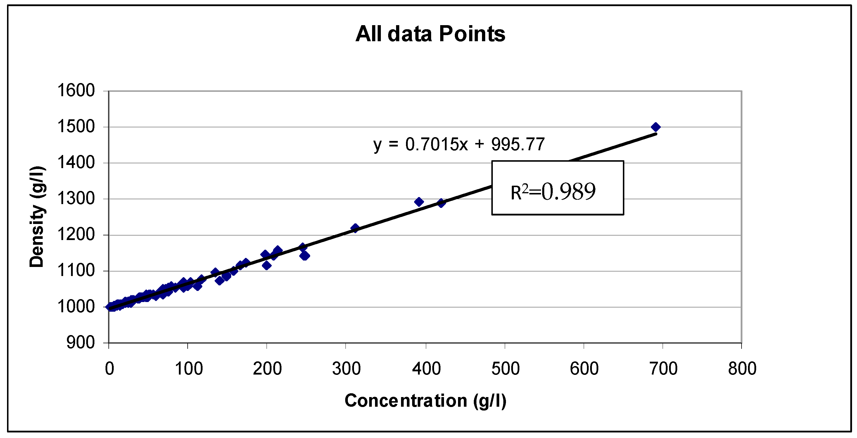
All Data			y = 0.7015x + 995.77	0.7015

summarizes the linear relations between the fluid density and various solute concentrations. Figure 1 shows the data points that Baxter and his colleagues measured in the lab and the corresponding linear regression lines. The slope of this linear regression line is based on all 115 data points, representing an overall density slope, and is 0.7015. This value is close to the ratio of density and concentration of “normal” sea water, which is approximately 0.7143, although the mixed data does not represent “normal” seawater. The difference is relatively small. A value of density slope (0.7) is also found in the literature (for example, [1]).

Regression analyses of some of the data shown in these papers [2,3] may lead to the following conclusions:

(1)

The fluid density is approximately proportional to the solute concentration.

(2)

Different solutes may have different relationships, or density slopes ranging from 0.54 to 0.75, between the concentrations and the fluid densities.

(3)

Most of the salts studied show similar slopes, with an average of 0.6775, while the linear regression line for all the sample data has an overall slope of 0.7015, which is quite close to the density slope for seawater 0.7143.

(4)

The density slopes are not proportional to the molecular weight of the salts.

4. Calculation of Density Slope from Salt Concentration

Based on the work of Baxter and his colleagues [2,3], we may approximate the relationship between fluid density and solute concentration, as in Equation (8) with a linear line:

$$\rho ={\rho }_f+E·C_s$$

(9)

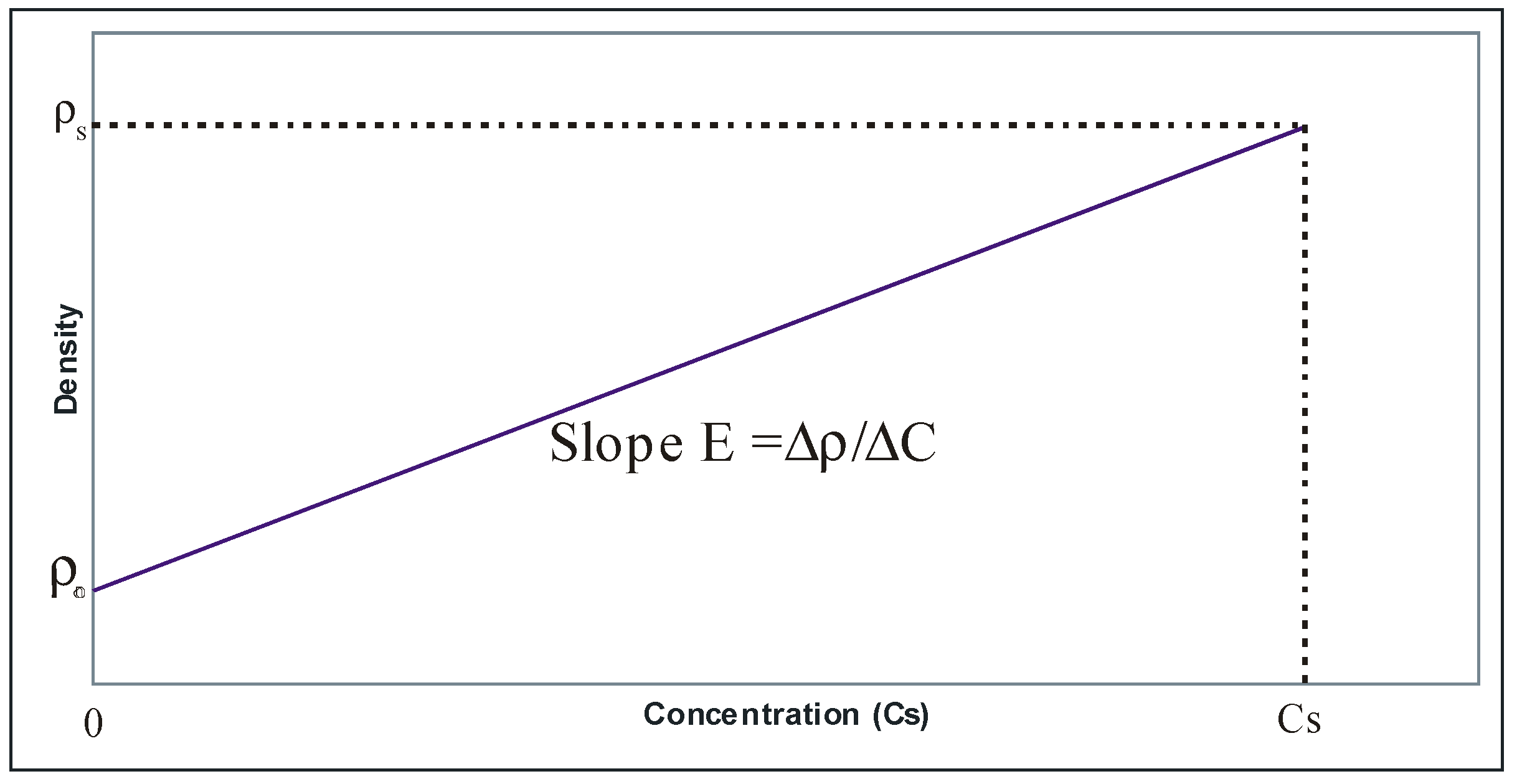
This linear relationship can also be shown graphically, as in Figure 2. In Equation (9), E is a dimensionless constant. It is sometimes referred to as the density slope [11]:

$$E=\frac{\Delta \rho }{\Delta C}=\frac{{\rho }_S-{\rho }_O}{C_S-C_O}$$

(10)

For typical sea water (ρ_s = 1025 kg/m³; its TDS or C_s = 35 kg/m³), assuming the freshwater density is ρ_o = 1000 kg/m³ and its salt concentration (C_o) = 0, we have:

$$E=\frac{{\rho }_S-{\rho }_O}{C_S-C_O}=\frac{1025-1000}{35.0}=\frac{25}{35}=0.7143$$

(11)

It should be noted that salinity is also a measure of the quantity of dissolved salts in sea water. It is formally defined as the total amount of dissolved solids in sea water in parts per thousand by weight where all the carbonate has been converted to oxide and all organic matter is completely oxidized [16]. A loose term for salinity is simply the total dissolved solids and is widely used. Hamann et al. [17] used a total salinity for density estimate based on the aqueous concentrations of major anions and cations: Na⁺, K⁺, Ca²⁺, Mg²⁺, Cl⁻, SO₄²⁻, HCO₃²⁻, and CO₃²⁻.

The density slope defined in Equation (11) is for seawater or seawater-related waters where TDS is considered as the solute concentration [11]. Kohfahl et al. [7] have shown that in general the density slopes, based on measured densities and TDS, have a range from 0.64 and 0.75 and the linear assumption between the fluid density and its TDS is valid up to approximately 400 g/L. Hamann et al. [17] found wider ranges of density slopes, from 0.61 to 0.81.

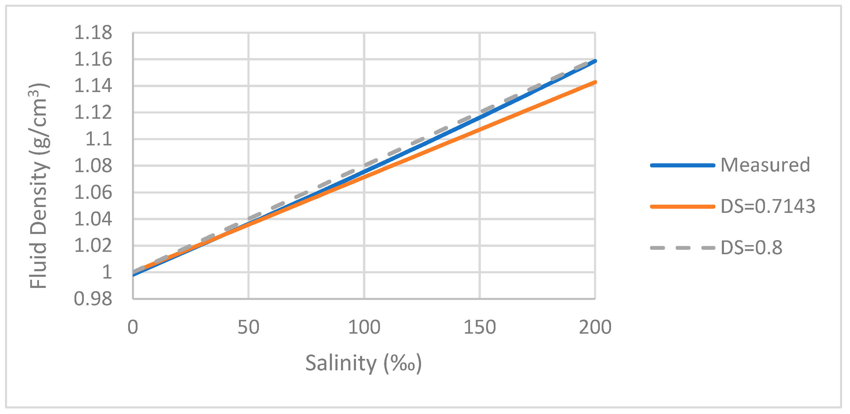
A comparison of the measured density at a temperature of 20 °C (www.unisense.com/files/pdf/diverse/seawat, accessed on 19 November2021) and estimated values based on a linear assumption with a constant density slop of 0.7143 (Equation (10)) is shown in Figure 3. It indicates that the density estimated based on the density slope of 0.7143 matches the measured values closely when the salinity is below 100‰. However, using a density slope of 0.7143 for saline water with salinity greater than 100‰ will underestimate the fluid density. For example, when the salinity is 200‰, the error in the fluid density calculation would be approximately 1.6%. For waters with higher salinity, the relationship between the salt concentration and fluid density shows some nonlinear behavior. A better estimate of water density may be achieved by using a greater density slope.

Table 2. Comparison of measured and estimated fluid density values (g/cm³).

Salinity	Fluid Density (g/cm3)
(‰)	Measured	DS = 0.7143	DS = 0.8
0	0.998	1	1
5	1.002	1.004	1.004
10	1.006	1.007	1.008
15	1.01	1.011	1.012
20	1.013	1.014	1.016
25	1.017	1.018	1.020
30	1.021	1.021	1.024
35	1.025	1.025	1.028
50	1.036	1.036	1.040
60	1.044	1.043	1.048
70	1.052	1.050	1.056
80	1.06	1.057	1.064
90	1.068	1.064	1.072
100	1.076	1.071	1.080
125	1.096	1.089	1.100
150	1.116	1.107	1.120
175	1.137	1.125	1.140
200	1.159	1.143	1.160

lists some of the estimated density values at 20 °C-based constant density slopes of 0.7143 and 0.8, respectively. At salinity 200‰, estimated density is 1.16 g/cm³, which is very close to the measured density value (1.1588 g/cm³). It should note that 0.8 was selected arbitrarily and it may not be the optimal value.

5. Calculation of Density Slope from Chloride Concentration Data

The traditional approach for monitoring the location and movement of saltwater contamination has been to periodically collect groundwater samples from discrete sampling horizons for the analysis of the chloride or dissolved solids concentration of the water. We can also use the concentration of other species present in the water as the input as long as the density slope is correctly specified, and it is assumed that a particular species can be used to represent how much dissolved solids are in the water. The assumption made here actually requires that the ratio of that particular species to TDS is constant. This assumption has been made implicitly in many software packages including SEAWAT [11]. The need to make this assumption is obvious and intuitive.

For example, chloride concentration is commonly measured in the field [18] and groundwater modeling [19,20] due to its abundance in seawater. Chloride ions are conservative, so they are not affected by significant oxidation or reduction reactions and do not form complexes with other ions unless the chloride concentration is very high [21]. In the natural world, the ratio of chloride to TDS varies from 5% to 55%. In coastal aquifers, the chloride concentration varies between 5 mg/L from infiltrated precipitation to 21,000 mg/L [22]. Chloride accounts for 55% of the salt in typical seawater [23]. Therefore, when chloride concentration is used to represent the solute concentration, as often seen in the literature, a 55% of chloride/TDS ratio is implicitly assumed.

An equation similar to Equation (11), which relates fluid density and TDS concentration, can be derived to relate the fluid density and chloride concentration:

$$\begin{gathered} \rho ={\rho }_f+E{C}_s \\ ={\rho }_f+\frac{\Delta \rho }{C_{s\left(TDS\right)}}{C}_{\left(TDS\right) }={\rho }_f+\frac{\Delta \rho }{C_{s\left(TDS\right)}\Delta \frac{C_{s\left(cl\right)}}{C_{s\left(cl\right)}}}{C}_{ \left(TDS\right) } \\ ={\rho }_f+\frac{\Delta \rho }{C_{s\left(Cl\right)}}\frac{C_{s\left(Cl\right)}}{C_{s \left(TDS\right)}}{C}_{\left(TDS\right)} \end{gathered}$$

(12)

Here, we assume that C_{s (TDS)} is the TDS concentration corresponding to seawater density and zero reference concentration. By assuming that the ratio of chloride concentration to TDS is a constant at approximately 0.55 for seawater, we have:

$$C_{\left(Cl\right)}=\frac{C_{s\left(Cl\right)}}{C_{s \left(TDS\right)}}{C}_{\left(TDS\right)}{}_{ }=0.55 C_{\left(TDS\right)}$$

(13)

So, the fluid density can be expressed as a function of chloride concentration data:

$$\rho ={\rho }_f+\frac{\Delta \rho }{C_{s\left(Cl\right)}}{C}_{\left(Cl\right) }$$

(14)

where C_{s (TDS)} is the TDS concentration corresponding to the maximum fluid density (seawater in our case) ρ_s; C_(Cl) is the chloride concentration, and C_s(Cl) is the chloride concentration corresponding to ρ_s. If we assume the chloride concentration in typical seawater is 19,000 mg/L [21], then the density slope is 25/19 = 1.3158, and the fluid density can be estimated from the chloride concentration as:

$$\rho ={\rho }_f+1.3158·C_{\left(Cl\right) }$$

(15)

It should be noted that (1) the application of Equation (14) requires the density slope to be modified appropriately, and (2) the ratio of chloride concentration to TDS concentration is assumed to be a constant. For normal seawater or seawater-related groundwater, this ratio is 55%.

The chloride/TDS ratio is not always 55% in natural waters. In most surface streams, chloride concentrations are lower than those of sulfate or bicarbonate [21].

Table 3. Measured chloride and TDS concentrations [24].

Well	Well Depth	Specific Conductance	Chloride	Sulfate	Bicarbonate	Sodium	Calsium	Magnesium	TDS	Chloride /TDS
Number	(ft)	μS/cm	mg/L	mg/L	mg/L	mg/L	mg/L	mg/L	mg/L
C-491	71	417	16	2	220	8	74	2	323	0.05
C-526	68	9660	3300	350	240	1300	310	148	5685	0.58
C-527	72	23,200	8300	1100	330	4200	480	503	15,033	0.55
C-1188	225	3720	1200	8	170	410	140	121	2107	0.57
C-1205	150	33,700	14,000	1800	300	6600	1200	940	24,900	0.56
C-1212	101	5350	1700	490	220	930	220	131	3714	0.46
L-1691	69	775	75	52	320	73	60	22	609	0.12
L-1973	225	781	120	28	290	73	39	37	598	0.20
L-2186	160	2470	560	240	250	300	130	55	1545	0.36
L-2187	154	1760	350	140	270	190	94	41	1095	0.32
L-2527	605	5800	1700	280	140	850	160	146	3303	0.51
L-2529	545	5940	2000	430	170	1100	140	162	4040	0.50
L-2820	241	2450	860	58	180	360	100	79	1659	0.52
L-2821	340	2350	610	190	160	320	72	74	1445	0.42
L-5649	128	976	200	27	270	66	100	23	690	0.29
L-5804	75	950	95	39	420	64	130	12	765	0.12
L-5842	180	937	120	44	320	70	94	17	667	0.18
L-5843	230	1260	270	27	250	110	63	43	773	0.35
L-5850	208	862	130	40	280	62	53	40	609	0.21

shows some of the water quality data collected from a number of relatively shallow groundwater monitoring wells located in Collier and Lee counties, Florida [24]. The chloride/TDS ratio varied significantly, from about 5% to 58%. It should be mentioned that the TDS values shown in the table were estimated based on the sum of major ions.

If the ratio of chloride concentration is not constant and values of chloride concentration are used as input for the modeling, then the amount of total dissolved solids cannot be determined, and nor can the fluid density. For example, if one sample contains 2000 mg/L of chloride and 20,000 mg/L of TDS, and another sample contains 11,000 mg/L of chloride but 20,000 mg/L of TDS, the equation using TDS will give the same density value (1014.3 g/L) for these two samples, although we know these two samples should have significantly different density values of 1002.63 g/L and 1014.47 g/L, respectively, as calculated from the chloride concentrations. It is apparent that the fluid density estimated from the chloride concentration for the second sample is close to the density value based on TDS when the chloride/TDS ratio is close to 55%.

Although TDS, as the salt concentration, is generally recommended as the solute species for fluid density calculations, we can basically use the concentration of any species in the solution to calculate fluid density if the ratio of the concentration of that species to TDS is a known or assumed constant. If the assumption of constant ratio is invalid or when the density–concentration relation is not linear, the equation of the state built in the modeling codes such as SEAWAT [11] may need to be revised and recompiled. For instance, in their study on the effects of chemical reactions on salt plume development, the authors of [25] incorporated the VOPO algorithm [14] into SEAWAT for fluid density calculations.

In SEAWAT, there are two sets of data in density slope calculations: concentration and fluid density. They have similar dimensions: M/L³. We may use different units, such as solute concentration as mg/L and fluid density as kg/m³, as long as they are consistent. Some commonly used values of solute concentrations and fluid density, as well as the corresponding density slope values, are listed in

Table 4. Commonly used density slope values.

(a) Assuming ρf = 1000 kg/m3, ρs = 1025 kg/m3
Solutes	Co	Cs	∆ρmax	∆Cmax	Density Slope
TDS in kg/m3	0	35	25	35	0.7143
TDS in lbs/ft3	0	2.185	25	2.185	11.4416
TDS in g/L	0	35	25	35	0.7143
TDS in mg/L	0	35,000	25	35,000	0.7143 × 10−3
Normalized TDS concentration	0	1	25	1	25
Chloride in kg/m3	0	19	25	19	1.3158
Chloride in lbs/ft3	0	1.1861	25	1.1861	21.077
Chloride in g/L	0	19	25	19	1.3158
Chloride in mg/L	0	19,000	25	19,000	1.3157 × 10−3
Normalized Chloride concentration	0	1	25	1	25
(b) Assuming ρf = 62.44 lbs/ft3, ρs = 64.001 lbs/ft3
Solutes	Co	Cs	∆ρmax	∆Cmax	Density Slope
TDS in kg/m3	0	35	1.561	35	0.0446
TDS in lbs/ft3	0	2.185	1.561	2.185	0.7144
TDS in g/L	0	35	1.561	35	0.0446
TDS in mg/L	0	35,000	1.561	35,000	4.46 × 10−5
Normalized TDS concentration	0	1	1.561	1	1.561
Chloride in kg/m3	0	19	1.561	19	0.08216
Chloride in lbs/ft3	0	1.1861	1.561	1.1861	1.3161
Chloride in g/L	0	19	1.561	19	0.08216
Chloride in mg/L	0	19,000	1.561	19000	8.216 × 10−5
Normalized Chloride concentration	0	1	1.561	1	1.561

.

It should be noted that each term in the partial differential equation for groundwater flow, like the one used in SEAWAT [11,26], has one and only one density term. Therefore, fluid density can be in any units (for example, kg/m³, g/L, lbs/ft³, etc.) as long as the unit is consistent. However, the choices of units of fluid density and solute concentration may affect the values of freshwater density and density slope.

6. Other Technical Considerations

As we have discussed, fluid density is preferably calculated from TDS concentration data. However, a problem often encountered is a lack of TDS concentration data. When field-measured TDS concentration data are not available, other means may be helpful to obtain the data needed.

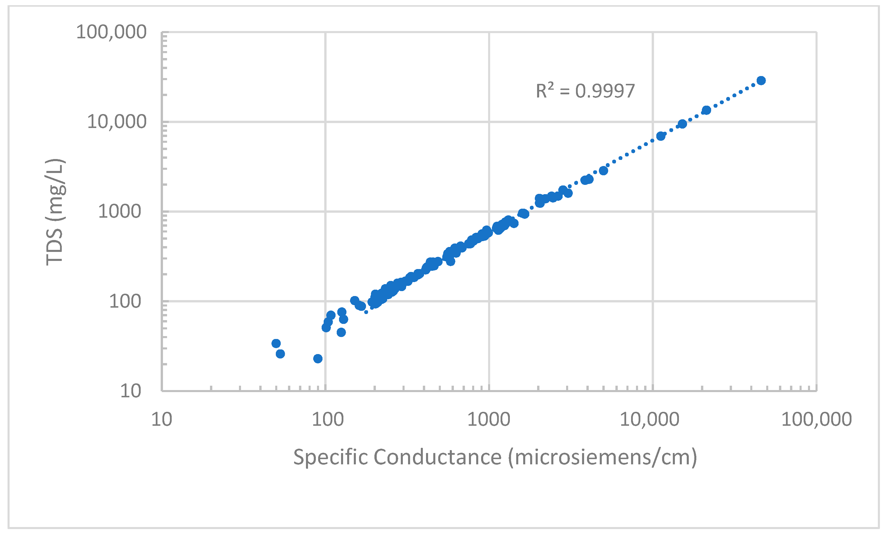
Field measurements of specific electric conductance of water in wells can be used to estimate TDS concentration. The development of high-tech-specific conductance meters allows for quick, inexpensive, and continuous in situ measurements of groundwater conductivity. The relationship between ionic concentration and specific conductance is fairly simple and direct in dilute solutions of a single salt [21]. The relationship between TDS and specific conductance can be complicated in the field, where many salts are present in the solution. However, the relationships between them are predominantly linear. A particular relationship can usually be established by the regression method using measured TDS and specific conductance data. Once this relationship is established, the TDS concentration can be estimated with reasonable accuracy.

Figure 4 shows the measured specific conductance versus TDS based on the groundwater samples collected in Orange County, Florida [27]. As shown, a linear relation can be easily observed.

Geophysical methods have been widely used for mapping the salinity distribution in coastal aquifers. Time-domain electromagnetic (TEM) soundings were made in Miami-Dade and southern Broward Counties to aid in mapping the landward extent of saltwater in the Biscayne aquifer [28]. Airborne electromagnetics (AEM) have been used to map the extent of saltwater intrusion in coastal areas in California [29]. TEM or AEM data can be converted into salinity or chloride data based on the same relationship.

Another method to estimate TDS concentrations is to establish a regression relationship between chloride and TDS concentrations using available data. After this relationship is established, the relationship can be used to estimate the TDS concentration for the samples that have only measured chloride concentration. If chloride concentration is desired as the modeling output, the same relationship should be used to back calculate chloride concentration.

Chloride concentration can also be simulated using the approach of multispecies solute transport. This feature has been implemented in many software packages, including SEAWAT [26]. Under this approach, the flow field is calculated based on the fluid density that is calculated using TDS concentrations and the solute transport of chloride or any other species is performed in the same simulation run.

Finally, it should be pointed out that there are many cases in which the influence of a variable fluid density can be ignored so a standard flow/solute transport approach (for example, the MODFLOW/MT3D approach) can be applied. This is especially true in the cases of shallow aquifers where the TDS concentration is low, and this is often where the concentration ratio of chloride/TDS is low.

7. Summary

The works of Baxter and his colleagues demonstrated the approximate linear relationship between fluid density and selected salts (halogen and alkali metals). A linear form of the equation of state (EOS) describing the fluid density and salt concentration has been widely adopted in density-drive modeling codes. Kohfahl et al. found that this linear approximation is valid for brines with TDS of up to 400 g/l. As shown, the error for using a constant density slope of 0.7143 is relatively small and acceptable when the TDS is less than 100 g/L, but the error increases when the TDS increases. For TDS values equal or greater than 200 g/L, a better match between the measured and estimated fluid densities may be achieved by using a greater density slope or using geochemical modeling.

The TDS of salt concentration is a better choice for fluid density estimations because all the solutes contribute to fluid density. Other species, such as dissolved chloride concentration, may also be used if the chloride/TDS ratio is assumed to be constant (e.g., 55% as for typical sea waters). The choice of concentration and freshwater density may affect the values of density slopes. Some commonly used density slope values are provided in this technical note for convenience.

Several methods (for example, specific conductance, TEM survey, etc.) can also be used indirectly to estimate the TDS or chloride concentration in groundwater. These methods often require calibration or statistical analyses.

References

- Pinder, G.F.; Cooper, H.H., Jr. A numerical technique for calculating the transient position of the saltwater front. Water Resour. Res. 1970, 6, 875–882. [Google Scholar] [CrossRef]
- Baxter, G.P.; Wallace, C.C. Changes in volume upon solution in water of the halogen salts of the alkali metals, II. J. Am. Chem. Soc. 1916, 38, 70–105. [Google Scholar] [CrossRef]
- Baxter, G.P. Changes in volume upon solution in water of the halogen salts of the alkalis. J. Am. Chem. Soc. 1911, 33, 922–940. [Google Scholar] [CrossRef] [Green Version]
- Bear, J. Conceptual and Mathematical Modeling, in Seawater Intrusion in Coastal Aquifers-Concepts, Methods and Practices; Bear, J., Cheng, H.D., Sorek, S., Ouazar, D., Herrera, I., Eds.; Kluwer Academic Publishers: Amsterdam, The Netherlands, 1999. [Google Scholar]
- Diersch, H.-J.G.; Kolditz, O. Variable-density flow and transport in porous media: Approach and challenges. Adv. Water Resour. 2002, 25, 899–944. [Google Scholar] [CrossRef]
- Diersch, H.-J.G. Consistent Velocity Approximation in the Finite-Element Simulation of Density Dependent Mass and Heat Transport Processes; FEFLOW-White Papers; WASY Gmbh: Berlin, Germany, 2005; Volume 1. [Google Scholar]
- Kohfahl, C.; Post, V.E.A.; Hamann, E.; Prommer, H.; Simmons, C.T. Validity and slope of the linear equation of state for natural brines in salt lake system. J. Hydrol. 2015, 523, 190–195. [Google Scholar] [CrossRef]
- Holzbecher, E. Modeling Density-Driven Flow in Porous Media; Springer: Berlin, Germany, 1998; 286p. [Google Scholar]
- Bear, J. Dynamics of Fluids in Porous Media; Elsevier Science: New York, NY, USA, 1972. [Google Scholar]
- Mao, X.; Prommer, H.; Barry, D.D.; Langevin, C.D.; Panteleit, B.; Li, L. Three-dimensional model for multi-component reactive transport with variable density groundwater flow. Environ. Model. Softw. 2016, 21, 615–628. [Google Scholar] [CrossRef]
- Guo, W.; Langevin, C.D. User’s guide to SEAWAT, A Computer Program for Simulation of Three-dimensional Variable Density Groundwater Flow, Techniques of Water-Resources Investigations of the U.S. Geol. Surv.; Book 6, Chapter 7; U.S. Geological Survey: Tallahassee, FL, USA, 2002; p. 77.
- Simpson, M.T.; Clement, T.P. Theoretical analysis of the worthiness of Henry and Elder problems as benchmarks of density-dependent groundwater flow models. Adv. Water Resour. 2003, 26, 17–31. [Google Scholar] [CrossRef]
- Hughes, J.D.; Sanford, W.E.; Vacher, H.L. Numerical simulation of double-diffusive finger convection. Water Resour. Res. 2005, 41, W01019. [Google Scholar] [CrossRef] [Green Version]
- Monnin, C. Density calculation and concentration scale conversion for natural waters. Comput. Geosci. 1994, 20, 1435–1445. [Google Scholar] [CrossRef]
- Kohfahl, C.; Post, V.E.A.; Hamann, E.; Prommer, H. The impact of hydrogeochemical reactions on densities. In Proceedings of the 22nd Salt Water Intrusion Meeting, Rio de Janeiro, Brazil, 17–22 June 2012; pp. 258–262. [Google Scholar]
- Chow, V.T. Handbook of Applied Hydrology; McGraw-Hill Book Company: New York, NY, USA, 1965. [Google Scholar]
- Hamann, E.; Post, V.; Kohfahl, C.; Prommer, H.; Simmons, C.T. Numerical investigation of coupled density-driven flow and hydrogeochemical processes below playas. Water Resour. Res. 2015, 51, 9338–9352. [Google Scholar] [CrossRef]
- Tsanis, I.K.; Song, L.F. Remediation of sea water intrusion: A case study. Groundw. Monit. Remediat. 2001, 21, 152–161. [Google Scholar] [CrossRef]
- Segol, G.; Pinder, G.F. Transient simulation of saltwater intrusion in southeastern Florida. Water Resour. Res. 1976, 12, 65–70. [Google Scholar] [CrossRef]
- Panday, S.; Huyakorn, P.S.; Robertson, J.B.; McGurk, B. A density-dependent flow and transport analysis of the effects of groundwater development in a freshwater lens of limited areal extent: The Geneva Area (Florida, USA) case study. J. Contam. Hydrol. 1993, 12, 329–354. [Google Scholar] [CrossRef]
- Hem, J.D. Study and Interpretation of the Chemical Characteristics of Natural Water, 3rd ed.; U.S. Geological Survey Water-Supply Paper 2254; U.S. Geological Survey: Tallahassee, FL, USA, 1992; p. 263.
- Boekelman, R.H.; Oude Essink, G.H.P.; Wang, J.; Ji, M.; Deyin, X.; Yang, Z. Salt-Water Intrusion Into Groundwater Systems. In Groundwater Contamination and Control-Environmental Science and Pollution Control Series; Zoller, V., Ed.; Marcel Dekker Inc.: New York, NY, USA, 1994; pp. 101–130. [Google Scholar]
- Drever, J. The Geochemistry of Nature Waters, 2nd ed.; Prentice Hall: Englewood Cliffs, NJ, USA, 1988; 437p. [Google Scholar]
- Schmerge, D. Distribution and Origin of Salinity in the Surficial and Intermediate Aquifer Systems, Southwestern Florida, U.S. Geol. Surv.; Water-Res.-Inv. Rep. 01-4159; U.S. Geological Survey: Tallahassee, FL, USA, 2001; 41p.
- Post, V.E.A.; Prommer, H. Multicomponent reactive transport simulation of the Elder problem: Effects of chemical reactions on salt plume development. Water Resour. Res. 2007, 43, 13. [Google Scholar] [CrossRef]
- Langevin, C.D.; Thore, D.T.; Dausman, A.M.; Sukop, M.C.; Guo, W. SEAWAT Version 4: A Computer Program for Simulation of Multi-Species Solute and Heat Transport: Techniques and Methods of U.S. Geol. Sur.; Book 6, Chapter A22; U.S. Geological Survey: Tallahassee, FL, USA, 2008; p. 39.
- Adamski, J.C.; German, E.R. Hydrogeology and Quality of Ground Water in Orange County, Florida, U.S.; Geol. Surv. Water-Res. Inv. Report; U.S. Geological Survey: Tallahassee, FL, USA, 2004; pp. 3–4257.
- Fitterman, D.V.; Prinos, S.T. Results of time-domain electromagnetic soundings in Miami-Dade and southern Broward Counties, Florida, U.S.; Geol. Surv. Open File Report; Geological Survey: Tallahassee, FL, USA, 2011; p. 289.
- Gottschalk, I.; Knight, R.; Asch, T.; Abraham, J.; Cannia, J. Using an airborne electromagnetic method to map saltwater intrusion in the northern Salinas Valley, California. SEG Libr. Geophys. 2020, 85, B119–B131. [Google Scholar] [CrossRef]
Figure 1.
Regression analysis of all data (data source: [3]).
Figure 2.
A general linear relationship between fluid density and salt concentrations.
Figure 3.
Comparison of measured and estimated fluid densities based on linear assumption (Equation (10)).
Figure 4.
Relation between specific conductance and TDS in groundwater. Samples collected from central Florida (after Adamski and German, 2004).