
Implementing an Operational Framework to Develop a Streamflow Duration Assessment Method: A Case Study from the Arid West United States

 , ,
, ,
Abstract
:1. Introduction
2. Materials and Methods
2.1. Streamflow Duration Classes
- Ephemeral reaches flow only in direct response to precipitation. Water typically flows only during and/or shortly after large precipitation events, the streambed is always above the water table, and stormwater runoff is the primary water source.
- Intermittent reaches contain sustained flowing water for only part of the year, typically during the wet season, where the streambed may be below the water table or where the snowmelt from surrounding uplands provides sustained flow. The flow may vary greatly with stormwater runoff.
- Perennial reaches contain flowing water continuously during a year of normal rainfall, often with the streambed located below the water table for most of the year. Groundwater typically supplies the baseflow for perennial reaches, but the baseflow may also be supplemented by stormwater runoff or snowmelt.
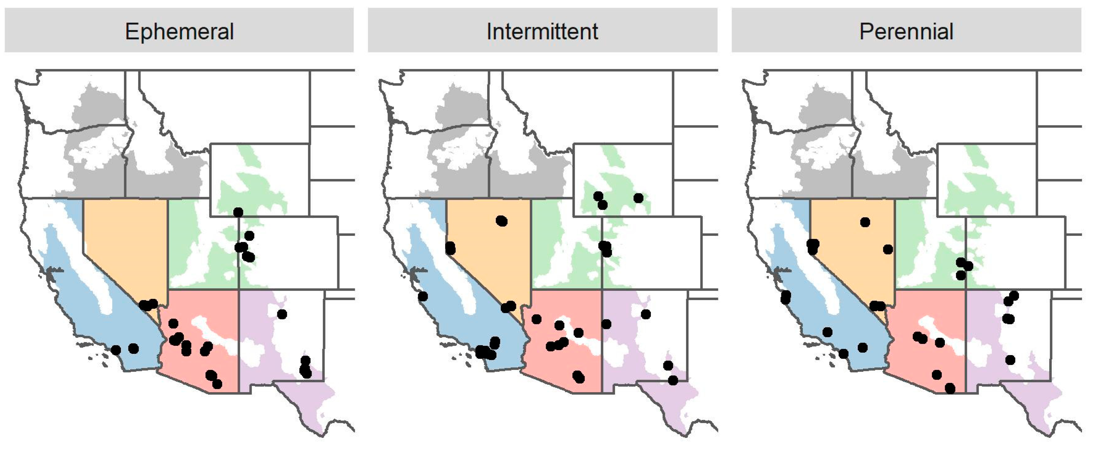
2.2. Study Area
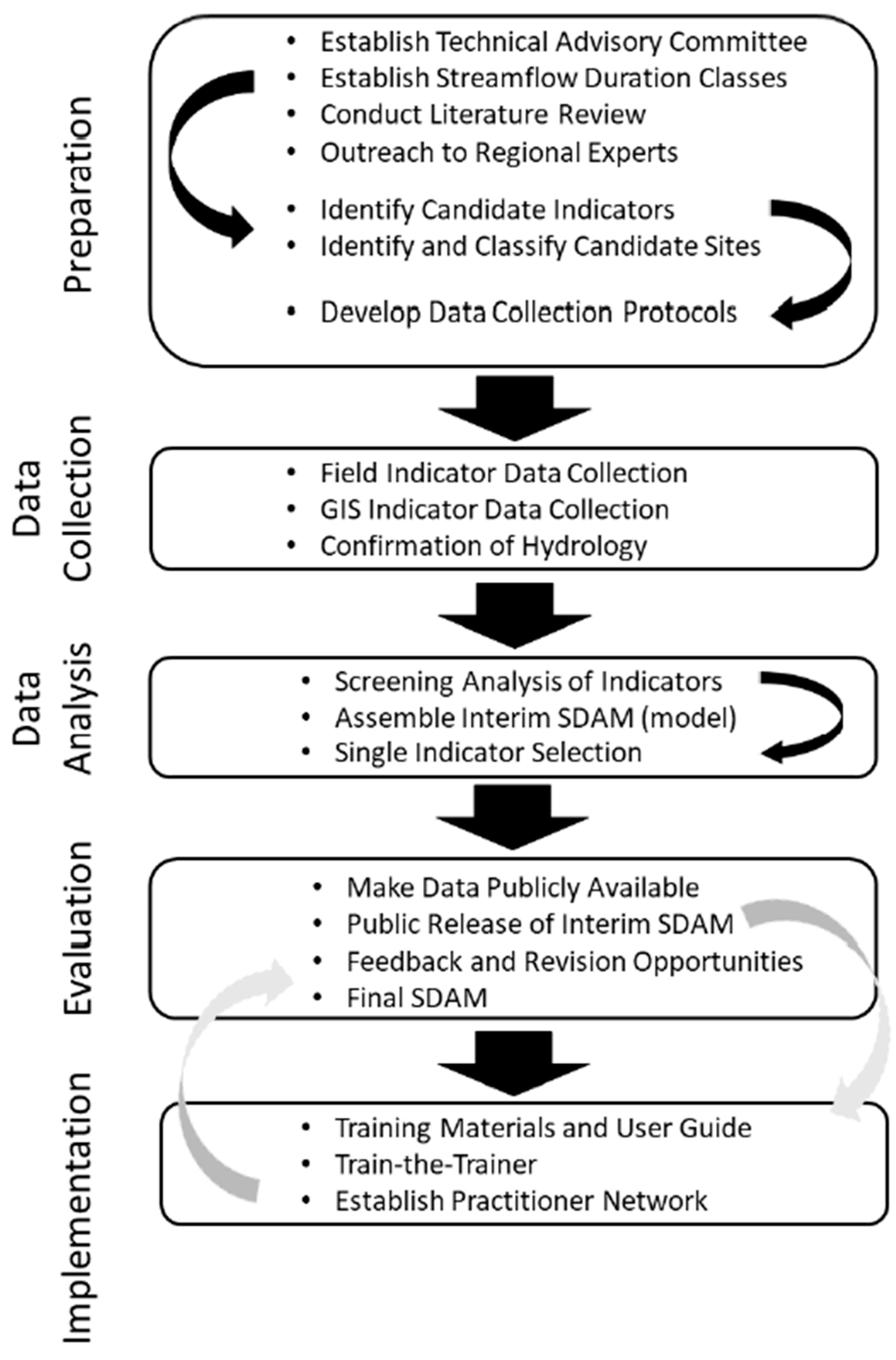
2.3. Preparation
2.3.1. Establish an Advisory Committee
2.3.2. Identify Candidate Indicators
- Consistency: Does the indicator consistently discriminate among flow duration classes (e.g., demonstrated in multiple studies)?
- Repeatability: Can different practitioners take similar measurements, given sufficient training and standardization?
- Defensibility: Does the indicator have a rational mechanistic relationship with flow duration, as either a response or a driver?
- Rapidness: Can the indicator be measured during a one-day reach-visit (even if subsequent lab analyses are required)?
- Objectivity: Does the indicator rely on objective (often quantitative) measures, as opposed to subjective judgments of practitioners?
- Robustness: Does human activity complicate indicator measurement or interpretation (e.g., poor water quality may affect the expression of some biological indicators)?
- Practicality: Can practitioners realistically sample the indicator with typical capacity, skills, and resources?
2.3.3. Identify candidate reaches
Goals in Selecting Reaches for Method Development
Classifying Streamflow Duration Based on Hydrologic Data
Selecting Reaches for Inclusion in This Study
2.3.4. Focus-Area Studies
2.4. Data Collection
2.4.1. Geomorphic Indicators
2.4.2. Hydrologic Indicators
2.4.3. Biological Indicators
2.4.4. Geospatial Data
2.5. Data Analysis
2.5.1. Calculation of Metrics
2.5.2. Metric Screening
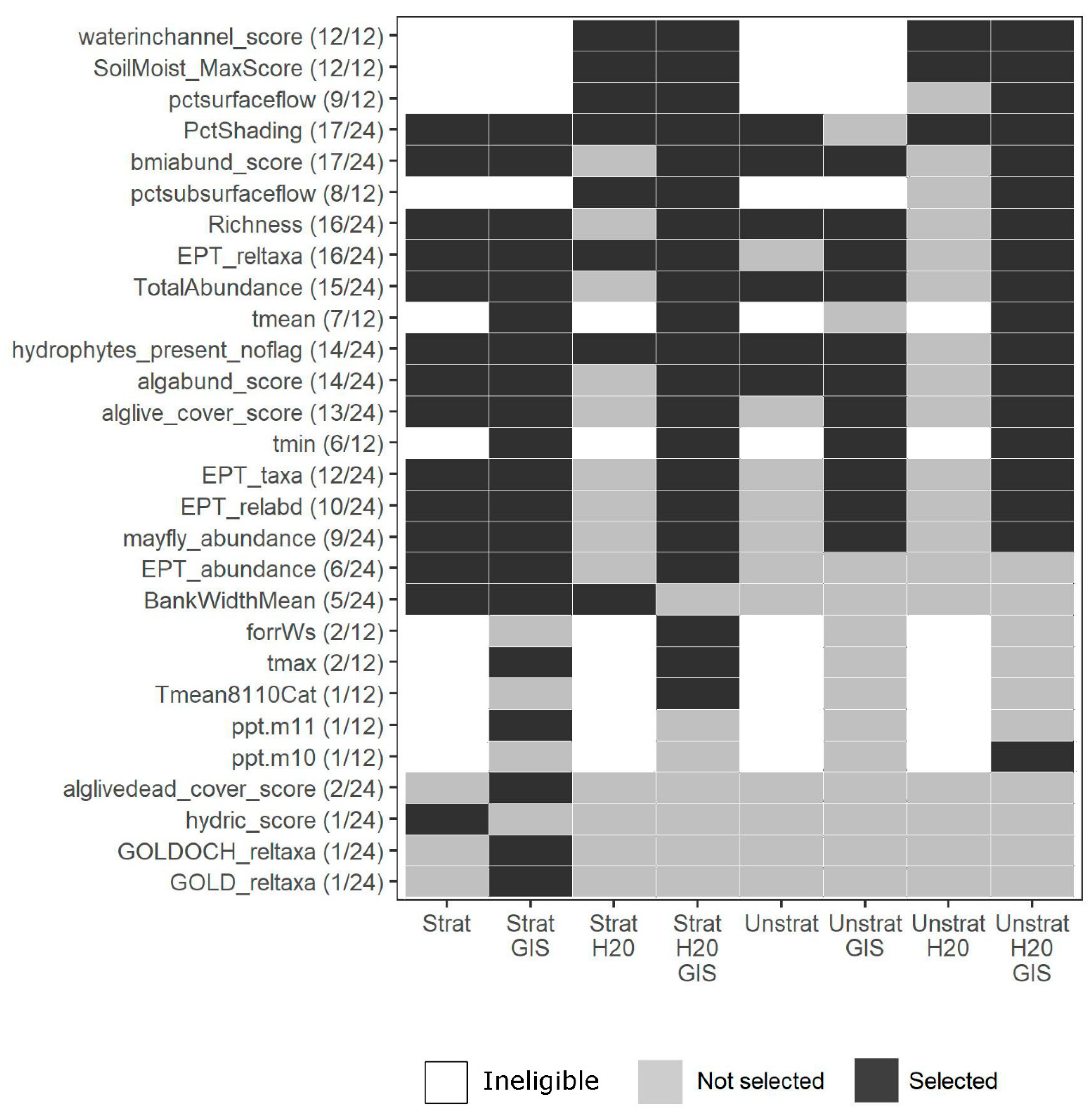
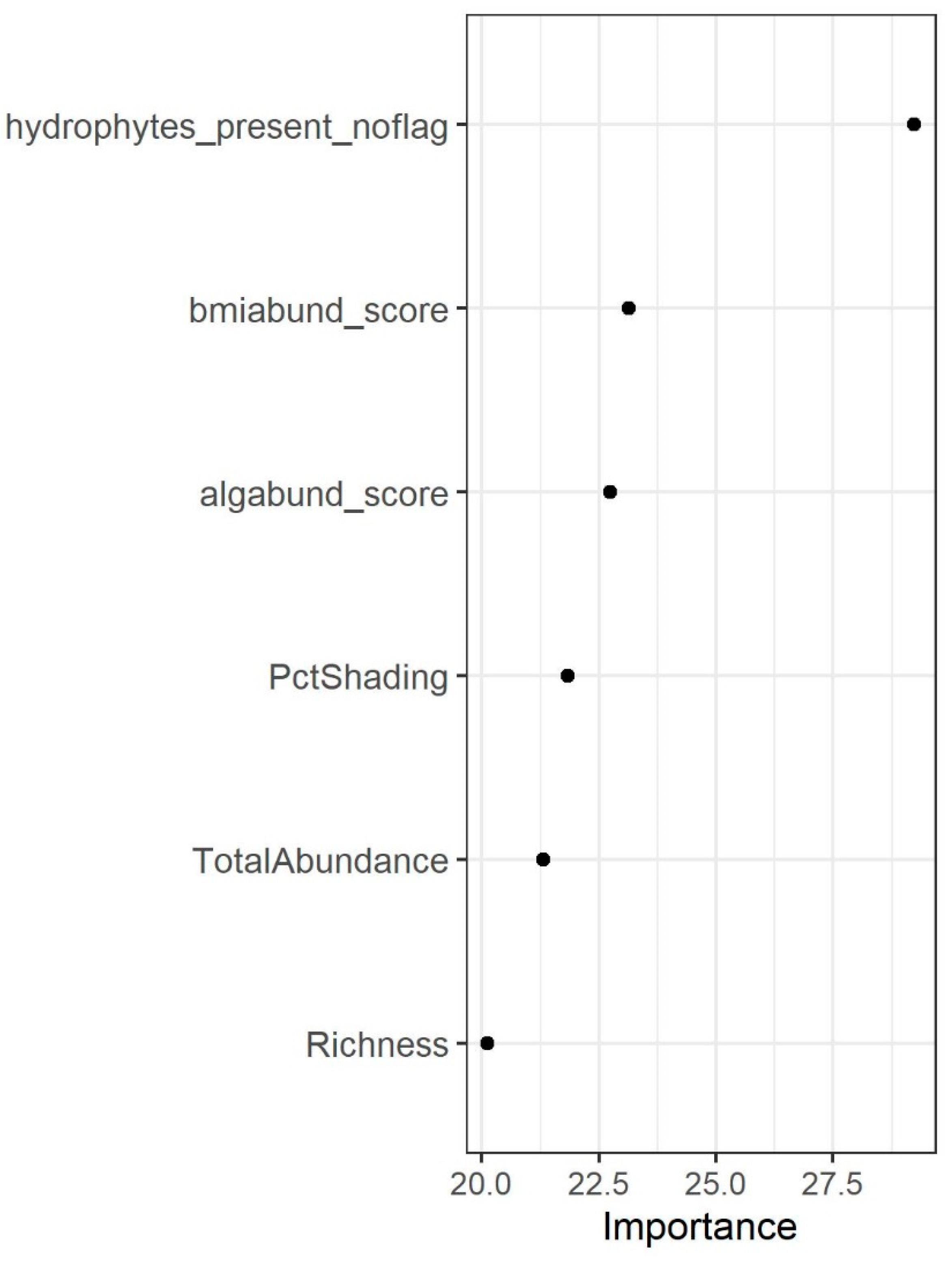
2.5.3. Metric Selection
- The full region-wide dataset, and
- Five separate datasets, one for each subregion shown in Figure 2.
- With or without considering geospatial metrics; and
- With or without considering metrics based on direct measures of water presence.
2.5.4. Model Calibration and Performance Evaluation
2.5.5. Selection of a Final Model
- Is a subregionally stratified approach warranted?
- Should we include geospatial metrics in the model?
- Should we include direct measures of water presence in the model?
- Should we use a single decision tree or a random forest model?
Refinement and Creation of a Final Beta Method
Refinement of Indicators
Increased Confidence Required for Classifications
Addition of Single Indicators
- Presence of live fish,
- Presence of live amphibians,
- Presence of any living aquatic vertebrate (fish, amphibians, or reptiles), and
- Live or dead (desiccated) algal cover on the streambed ≥10%.
2.5.6. Evaluation of the Final Beta SDAM and Comparison with Other SDAMs Used in Portions of the AW
2.6. Application to Two Focus-Area Studies
3. Results
3.1. Identification of Candidate Indicators
3.2. Identification of Candidate Study Reaches
3.3. Data Collection
3.4. Data Analysis
3.4.1. Metric Screening
3.4.2. Metric Selection
3.4.3. Model Calibration and Performance Evaluation
3.4.4. Selection of a Final Model
3.4.5. Refinement and Creation of a Final Beta Method
Refinement of Indicators
Riparian Vegetation
Aquatic Invertebrate Abundance
Aquatic Invertebrate Composition
Algal Abundance
Increased Confidence Required for Classifications
Addition of Single Indicators
3.4.6. Evaluation of the Final Beta SDAM and Comparison with Other SDAMs Used in Portions of the AW
3.5. Application to Two Focus-Area Studies
4. Discussion
4.1. The Beta SDAM AW Can Support a Range of Management and Monitoring Needs
4.2. Strengths and Limitations of the Beta SDAM AW
4.3. Indicators Used in the Beta SDAM AW Have a Strong Conceptual Link to Streamflow Duration
4.3.1. Hydrophytic Plants
4.3.2. Aquatic Invertebrate Abundance and Composition
4.3.3. Algal Indicators
4.4. Lessons Learned about SDAM Development
4.4.1. Engage End-Users throughout the Development Process
4.4.2. Statistical Complexity Does Not Need to Create a Barrier for End-Users
4.4.3. Poor Documentation of Ephemeral Streams Creates Major but Surmountable Challenges
4.4.4. Make the Best Use of Local Expertise
4.4.5. Recognize the True Complexity of Streamflow Duration Gradients
4.5. Future Research and Method Development Needs
4.5.1. Investigate the Persistence of Indicator Expression at Reaches That Have Undergone Changes in Streamflow Duration
4.5.2. Address Challenges Created by the Dependence on Taxonomic Expertise
4.5.3. Get More and Better Hydrologic Data
4.5.4. Identify Positive Indicators of Ephemeral Streamflow Duration
5. Conclusions
Supplementary Materials
Author Contributions
Funding
Institutional Review Board Statement
Informed Consent Statement
Data Availability Statement
Acknowledgments
Conflicts of Interest
Acronyms and Abbreviations
| ALI | At least intermittent |
| AW | Arid West |
| AZ | Arizona |
| CA | California |
| CO | Colorado |
| Corps | United States Army Corps of Engineers |
| EPT | Ephemeroptera, Plecoptera, and Trichoptera taxa |
| EvALI | Ephemeral versus at least intermittent |
| FACW | Facultative-Wet wetland plant indicator status |
| GIS | Geographic Information System |
| GOLD | Gastropoda, Oligochaeta, and Diptera taxa |
| GOLDOCH | Gastropoda, Oligochaeta, Diptera, Odonata, Coleoptera, and Heteroptera taxa |
| H2O | Direct measures of water presence |
| MDA | Mean decrease accuracy (a measure of variable importance in random forest models) |
| MDS | Multidimensional scaling |
| MT | Montana |
| NHD | National Hydrography Dataset |
| NM | New Mexico |
| NMI | Need more information |
| NV | Nevada |
| OBL | Obligate wetland plant indicator status |
| OCH | Odonata, Coleoptera, and Heteroptera taxa |
| PNW | Pacific Northwest |
| PRISM | Parameter-elevation Regressions on Independent Slope Models (a repository of modeled climate data) |
| PvIvE | Perennial versus intermittent versus ephemeral |
| PvNP | Perennial versus non-perennial |
| RSC | Regional Steering Committee |
| SDAM | Streamflow duration assessment method |
| SDAM AW | Streamflow duration assessment method for the Arid West |
| SDAM NM | Streamflow duration assessment method for New Mexico |
| SDAM PNW | Streamflow duration assessment method for the Pacific Northwest |
| STIC | Stream Temperature, Intermittence, and Conductivity logger |
| TX | Texas |
| USEPA | United States Environmental Protection Agency |
| USGS | United States Geological Survey |
| UT | Utah |
| WY | Wyoming |
References
- Fritz, K.M.; Nadeau, T.-L.; Kelso, J.E.; Beck, W.S.; Mazor, R.D.; Harrington, R.A.; Topping, B.J. Classifying Streamflow Duration: The Scientific Basis and an Operational Framework for Method Development. Water 2020, 12, 2545. [Google Scholar] [CrossRef] [PubMed]
- Granato, G.E.; Ries III, K.G.; Steeves, P.A. Compilation of Streamflow Statistics Calculated from Daily Mean Streamflow Data Collected during Water Years 1901–2015 for Selected U.S. Geological Survey Streamgages; U.S. Geological Survey Open-File Report 2017-1108; U.S. Geological Survey: Reston, VA, USA, 2017; p. 17. Available online: https://pubs.er.usgs.gov/publication/ofr20171108 (accessed on 20 November 2021).
- Zimmer, M.A.; Kaiser, K.E.; Blaszczak, J.R.; Zipper, S.C.; Hammond, J.C.; Fritz, K.M.; Costigan, K.H.; Hosen, J.; Godsey, S.E.; Allen, G.H.; et al. Zero or Not? Causes and Consequences of Zero-flow Stream Gage Readings. WIREs Water 2020, 7. [Google Scholar] [CrossRef] [PubMed]
- Anning, D.W.; Parker, J.T.C. Predictive Models of the Hydrological Regime of Unregulated Streams in Arizona; U.S. Geological Survey Open-File Report; US Geological Survey: Tucson, AZ, USA, 2009; p. 33. Available online: https://pubs.usgs.gov/of/2009/1269/ (accessed on 20 November 2021).
- Reynolds, L.V.; Shafroth, P.B.; LeRoy Poff, N. Modeled Intermittency Risk for Small Streams in the Upper Colorado River Basin under Climate Change. J. Hydrol. 2015, 523, 768–780. [Google Scholar] [CrossRef]
- Sando, R.; Blasch, K.W. Predicting Alpine Headwater Stream Intermittency: A Case Study in the Northern Rocky Mountains. Ecohydrol. Hydrobiol. 2015, 15, 68–80. [Google Scholar] [CrossRef]
- Lane, B.A.; Dahlke, H.E.; Pasternack, G.B.; Sandoval-Solis, S. Revealing the Diversity of Natural Hydrologic Regimes in California with Relevance for Environmental Flows Applications. J. Am. Water Resour. Assoc. 2017, 53, 411–430. [Google Scholar] [CrossRef] [Green Version]
- Merritt, A.; Lane, B.; Hawkins, C. Classification and Prediction of Natural Streamflow Regimes in Arid Regions of the USA. Water 2021, 13, 380. [Google Scholar] [CrossRef]
- Busch, M.H.; Costigan, K.H.; Fritz, K.M.; Datry, T.; Krabbenhoft, C.A.; Hammond, J.C.; Zimmer, M.; Olden, J.D.; Burrows, R.M.; Dodds, W.K.; et al. What’s in a Name? Patterns, Trends, and Suggestions for Defining Non-Perennial Rivers and Streams. Water 2020, 12, 1980. [Google Scholar] [CrossRef] [PubMed]
- Costigan, K.H.; Jaeger, K.L.; Goss, C.W.; Fritz, K.M.; Goebel, P.C. Understanding Controls on Flow Permanence in Intermittent Rivers to Aid Ecological Research: Integrating Meteorology, Geology and Land Cover: Integrating Science to Understand Flow Intermittence. Ecohydrology 2016, 9, 1141–1153. [Google Scholar] [CrossRef]
- Leasure, D.R.; Magoulick, D.D.; Longing, S.D. Natural Flow Regimes of the Ozark-Ouachita Interior Highlands Region. River Res. Applic. 2016, 32, 18–35. [Google Scholar] [CrossRef]
- Texas Commission on Environmental Quality. Chapter 307—Texas Surface Water Quality Standards; Rule Project No. 2016-002-307-OW; Texas Commission on Environmental Quality: Austin, TX, USA, 2018; p. 212.
- Poff, N.L.; Ward, J.V. Implications of Streamflow Variability and Predictability for Lotic Community Structure: A Regional Analysis of Streamflow Patterns. Can. J. Fish. Aquat. Sci. 1989, 46, 1805–1818. [Google Scholar] [CrossRef]
- Winter, T.C.; Harvey, J.W.; Franke, O.L.; Alley, W.M. Groundwater and Surface Water: A Single Resource; US Geological Survey: Denver, CO, USA, 1998; p. 79.
- Chadwick, M.A.; Huryn, A.D. Role of Habitat in Determining Macroinvertebrate Production in an Intermittent-Stream System. Freshw. Biol. 2007, 52, 240–251. [Google Scholar] [CrossRef]
- Fritz, K.M.; Johnson, B.R.; Walters, D.M. Physical Indicators of Hydrologic Permanence in Forested Headwater Streams. J. N. Am. Benthol. Soc. 2008, 27, 690–704. [Google Scholar] [CrossRef]
- Austin, B.J.; Strauss, E.A. Nitrification and Denitrification Response to Varying Periods of Desiccation and Inundation in a Western Kansas Stream. Hydrobiologia 2011, 658, 183–195. [Google Scholar] [CrossRef]
- Datry, T. Benthic and Hyporheic Invertebrate Assemblages along a Flow Intermittence Gradient: Effects of Duration of Dry Events: River Drying and Temporary River Invertebrates. Freshw. Biol. 2012, 57, 563–574. [Google Scholar] [CrossRef]
- Schriever, T.A.; Bogan, M.T.; Boersma, K.S.; Cañedo-Argüelles, M.; Jaeger, K.L.; Olden, J.D.; Lytle, D.A. Hydrology Shapes Taxonomic and Functional Structure of Desert Stream Invertebrate Communities. Freshw. Sci. 2015, 34, 399–409. [Google Scholar] [CrossRef] [Green Version]
- Wipfli, M.S.; Richardson, J.S.; Naiman, R.J. Ecological Linkages Between Headwaters and Downstream Ecosystems: Transport of Organic Matter, Invertebrates, and Wood Down Headwater Channels1: Ecological Linkages Between Headwaters and Downstream Ecosystems. JAWRA J. Am. Water Resour. Assoc. 2007, 43, 72–85. [Google Scholar] [CrossRef]
- Nadeau, T.-L.; Rains, M.C. Hydrological Connectivity Between Headwater Streams and Downstream Waters: How Science Can Inform Policy. JAWRA J. Am. Water Resour. Assoc. 2007, 43, 118–133. [Google Scholar] [CrossRef]
- Stubbington, R.; Bogan, M.T.; Bonada, N.; Boulton, A.J.; Datry, T.; Leigh, C.; Vander Vorste, R. The Biota of Intermittent Rivers and Ephemeral Streams: Aquatic Invertebrates. In Intermittent Rivers and Ephemeral Streams; Elsevier: Amsterdam, The Netherlands, 2017; pp. 217–243. ISBN 978-0-12-803835-2. [Google Scholar]
- Steward, A.L.; Langhans, S.D.; Corti, R.; Datry, T. The Biota of Intermittent Rivers and Ephemeral Streams: Terrestrial and Semiaquatic Invertebrates. In Intermittent Rivers and Ephemeral Streams; Elsevier: Amsterdam, The Netherlands, 2017; p. 245. ISBN 978-0-12-803835-2. [Google Scholar]
- Leigh, C.; Datry, T. Drying as a Primary Hydrological Determinant of Biodiversity in River Systems: A Broad-Scale Analysis. Ecography 2017, 40, 487–499. [Google Scholar] [CrossRef] [Green Version]
- Nadeau, T.-L.; Leibowitz, S.G.; Wigington, P.J.; Ebersole, J.L.; Fritz, K.M.; Coulombe, R.A.; Comeleo, R.L.; Blocksom, K.A. Validation of Rapid Assessment Methods to Determine Streamflow Duration Classes in the Pacific Northwest, USA. Environ. Manag. 2015, 56, 34–53. [Google Scholar] [CrossRef] [PubMed]
- U.S. Army Corps of Engineers; U.S. Environmental Protection Agency. Notice of Availability of the Beta Streamflow Duration Assessment Method for the Arid West; U.S. Army Corps of Engineers: Washington, DC, USA, 2021. Available online: https://www.epa.gov/sites/production/files/2021-03/documents/joint_spd_pn_sdam_11mar21_final_508.pdf (accessed on 20 November 2021).
- Nadeau, T.-L. Streamflow Duration Assessment Method for the Pacific Northwest; EPA 910-K-14-001; U.S. Environmental Protection Agency: Washington, DC, USA, 2015; p. 36. Available online: https://www.epa.gov/sites/default/files/2016-01/documents/streamflow_duration_assessment_method_pacific_northwest_2015.pdf (accessed on 20 November 2021).
- U.S. Army Corps of Engineers. Regional Supplement to the Corps of Engineers Wetland Delineation Manual: Arid West Region (Version 2.0); Regional Supplements to the Corps of Engineers Wetland Delineation Manual; U.S. Army Engineer Research and Development Center: Vicksburg, MS, USA; Army Engineer Research and Development Center: Hanover, NH, USA, 2008; p. 135.
- Gasith, A.; Resh, V.H. Streams in Mediterranean Climate Regions: Abiotic Influences and Biotic Responses to Predictable Seasonal Events. Annu. Rev. Ecol. Syst. 1999, 30, 51–81. [Google Scholar] [CrossRef] [Green Version]
- Goodrich, D.C.; Kepner, W.G.; Levick, L.R.; Wigington, P.J. Southwestern Intermittent and Ephemeral Stream Connectivity. J. Am. Water Resour. Assoc. 2018, 54, 400–422. [Google Scholar] [CrossRef] [Green Version]
- Messager, M.L.; Lehner, B.; Cockburn, C.; Lamouroux, N.; Pella, H.; Snelder, T.; Tockner, K.; Trautmann, T.; Watt, C.; Datry, T. Global Prevalence of Non-Perennial Rivers and Streams. Nature 2021, 594, 391–397. [Google Scholar] [CrossRef] [PubMed]
- Sleeter, B.M.; Wilson, T.S.; Soulard, C.E.; Liu, J. Estimation of Late Twentieth Century Land-Cover Change in California. Environ. Monit. Assess. 2011, 173, 251–266. [Google Scholar] [CrossRef] [PubMed]
- Mackun, P. Fast Growth in the Desert Southwest Continues. In America Counts: Stories Behind the Numbers US Census Bureau; 2019. Available online: https://www.census.gov/library/stories/2019/02/fast-growth-in-desert-southwest-continues.html (accessed on 20 November 2021).
- New Mexico Environment Department (NMED). Hydrology Protocol for the Determination of Uses Supported by Ephemeral, Intermittent, and Perennial Waters; Surface Water Quality Bureau, New Mexico Environment Department: Albuquerque, NM, USA, 2011; p. 35.
- McCune, K.; Mazor, R.D. Review of Flow Duration Methods and Indicators of Flow Duration in the Scientific Literature: Arid Southwest; SCCWRP Technical Report 1063; Southern California Coastal Water Research Project: Costa Mesa, CA, USA, 2019; p. 90. Available online: https://ftp.sccwrp.org/pub/download/DOCUMENTS/TechnicalReports/1063_FlowMethodsReview.pdf (accessed on 20 November 2021).
- Lichvar, R.W.; Banks, D.L.; Kirchner, W.N.; Melvin, N.C. The National Wetland Plant List: 2016 Wetland Ratings. Phytoneutron 2016, 30, 1–17. [Google Scholar]
- Hill, R.A.; Weber, M.H.; Leibowitz, S.G.; Olsen, A.R.; Thornbrugh, D.J. The Stream-Catchment (StreamCat) Dataset: A Database of Watershed Metrics for the Conterminous United States. J. Am. Water Resour. Assoc. 2016, 52, 120–128. [Google Scholar] [CrossRef]
- Hart, E.; Bell, K. Prism: Access Data from the Oregon State Prism Climate Project; R Package Version 0.0.6; 2015; Available online: https://www.researchgate.net/publication/308963991_prism_Access_data_from_the_Oregon_State_Prism_climate_project (accessed on 20 November 2021).
- Omernik, J.M.; Griffith, G.E. Ecoregions of the Conterminous United States: Evolution of a Hierarchical Spatial Framework. Environ. Manag. 2014, 54, 1249–1266. [Google Scholar] [CrossRef] [PubMed]
- Jaeger, K.L.; Olden, J.D. Electrical Resistance Sensor Arrays as a Means to Quantify Longitudinal Connectivity of Rivers. River Res. Applic. 2012, 28, 1843–1852. [Google Scholar] [CrossRef]
- Chapin, T.P.; Todd, A.S.; Zeigler, M.P. Robust, Low-Cost Data Loggers for Stream Temperature, Flow Intermittency, and Relative Conductivity Monitoring. Water Resour. Res. 2014, 50, 6542–6548. [Google Scholar] [CrossRef]
- McKay, L.; Bondelid, T.; Dewald, T.; Johnson, J.; Moore, R.; Rea, A. NHDPlus Version 2: User Guide; U.S. Geological Survey: Reston, VA, USA, 2014; p. 173.
- Oksanen, J.; Blanchet, F.G.; Friendly, M.; Kindt, R.; Legendre, P.; McGlinn, D.; Minchin, P.R.; O’Hara, R.B.; Simpson, G.L.; Solymos, P.; et al. Vegan: Community Ecology Package; R Package Version 2.5-6; 2019; Available online: https://CRAN.R-project.org/package=vegan (accessed on 20 November 2021).
- Stoddard, J.L.; Herlihy, A.T.; Peck, D.V.; Hughes, R.M.; Whittier, T.R.; Tarquinio, E. A Process for Creating Multimetric Indices for Large-Scale Aquatic Surveys. J. N. Am. Benthol. Soc. 2008, 27, 878–891. [Google Scholar] [CrossRef]
- Hawkins, C.P.; Cao, Y.; Roper, B. Method of Predicting Reference Condition Biota Affects the Performance and Interpretation of Ecological Indices. Freshw. Biol. 2010, 55, 1066–1085. [Google Scholar] [CrossRef]
- Cao, Y.; Hawkins, C.P. The Comparability of Bioassessments: A Review of Conceptual and Methodological Issues. J. N. Am. Benthol. Soc. 2011, 30, 680–701. [Google Scholar] [CrossRef] [Green Version]
- Mazor, R.D.; Rehn, A.C.; Ode, P.R.; Engeln, M.; Schiff, K.C.; Stein, E.D.; Gillett, D.J.; Herbst, D.B.; Hawkins, C.P. Bioassessment in Complex Environments: Designing an Index for Consistent Meaning in Different Settings. Freshw. Sci. 2016, 35, 249–271. [Google Scholar] [CrossRef]
- Liaw, A.; Wiener, M. Classification and Regression by RandomForest. R News 2002, 2, 18–22. [Google Scholar]
- Kuhn, M. Caret: Classification and Regression Training; R Package Version 6.0-86; 2020; Available online: https://CRAN.R-project.org/package=caret (accessed on 20 November 2021).
- Therneau, T.; Atkinson, B. Rpart: Recursive Partitioning and Regression Trees; R Package Version 4.1-15; 2019; Available online: https://CRAN.R-project.org/package=rpart (accessed on 20 November 2021).
- Topping, B.J.D.; Nadeau, T.-L.; Turaski, M.R. Oregon Streamflow Duration Assessment Method—Interm Version; U.S. Environmental Protection Agency: Portland, OR, USA, 2009; p. 60. Available online: https://www.epa.gov/sites/production/files/201601/documents/streamflow_duration_assessment_method_oregon_interim_2009.pdf (accessed on 20 November 2021).
- Dorney, J.; Russell, P. North Carolina Division of Water Quality Methodology for Identification of Intermittent and Perennial Streams and Their Origins. In Wetland and Stream Rapid Assessments; Elsevier: Amsterdam, The Netherlands, 2018; pp. 273–279. ISBN 978-0-12-805091-0. [Google Scholar]
- Gallart, F.; Llorens, P.; Latron, J.; Cid, N.; Rieradevall, M.; Prat, N. Validating Alternative Methodologies to Estimate the Regime of Temporary Rivers When Flow Data Are Unavailable. Sci. Total. Environ. 2016, 565, 1001–1010. [Google Scholar] [CrossRef] [PubMed]
- Gallart, F.; Cid, N.; Latron, J.; Llorens, P.; Bonada, N.; Jeuffroy, J.; Jiménez-Argudo, S.-M.; Vega, R.-M.; Solà, C.; Soria, M.; et al. TREHS: An Open-Access Software Tool for Investigating and Evaluating Temporary River Regimes as a First Step for Their Ecological Status Assessment. Sci. Total. Environ. 2017, 607–608, 519–540. [Google Scholar] [CrossRef]
- Ohio EPA. Field Evaluation Manual for Ohio’s Primary Headwater Habitat Streams; Version 3.0; Ohio EPA Division of Surface Water: Columbus, OH, USA, 2012; p. 117. Available online: https://epa.ohio.gov/portals/35/wqs/headwaters/PHWHManual_2012.pdf (accessed on 20 November 2021).
- Svec, J.R.; Kolka, R.K.; Stringer, J.W. Defining Perennial, Intermittent, and Ephemeral Channels in Eastern Kentucky: Application to Forestry Best Management Practices. For. Ecol. Manag. 2005, 214, 170–182. [Google Scholar] [CrossRef]
- Fritz, K.M.; Johnson, B.R.; Walters, D.M. Field Operations Manual for Assessing the Hydrologic Permanence and Ecological Condition of Headwater Streams; U.S. Environmental Protection Agency, Ed.; Office of Research and Development: Washington, DC, USA, 2006; p. 151. Available online: https://cfpub.epa.gov/si/si_public_record_report.cfm?Lab=NERL&dirEntryId=159984 (accessed on 20 November 2021).
- Greenwell, B.M. Pdp: An R Package for Constructing Partial Dependence Plots. R J. 2017, 9, 421–436. [Google Scholar] [CrossRef] [Green Version]
- Fritz, K.M.; Wenerick, W.R.; Kostich, M.S. A Validation Study of a Rapid Field-Based Rating System for Discriminating Among Flow Permanence Classes of Headwater Streams in South Carolina. Environ. Manag. 2013, 52, 1286–1298. [Google Scholar] [CrossRef]
- Mazor, R.D. Bioassessment Survey of the Stormwater Monitoring Coalition: Workplan for the Years 2021 through 2015; Version 1.0; Southern California Coastal Water Research Project: Costa Mesa, CA, USA, 2021; p. 52. Available online: https://ftp.sccwrp.org/pub/download/DOCUMENTS/TechnicalReports/1174_SMCBioassessmentWorkplan.pdf (accessed on 20 November 2021).
- Bêche, L.A.; Resh, V.H. Biological Traits of Benthic Macroinvertebrates in California Mediterranean-Climate Streams: Long-Term Annual Variability and Trait Diversity Patterns. Fundam. Appl. Limnol. 2007, 169, 1–23. [Google Scholar] [CrossRef]
- Bogan, M.T.; Boersma, K.S.; Lytle, D.A. Flow Intermittency Alters Longitudinal Patterns of Invertebrate Diversity and Assemblage Composition in an Arid-Land Stream Network: Intermittent Flow Alters Longitudinal Patterns. Freshw. Biol. 2013, 58, 1016–1028. [Google Scholar] [CrossRef]
- Boersma, K.S.; Dee, L.E.; Miller, S.J.; Bogan, M.T.; Lytle, D.A.; Gitelman, A.I. Linking Multidimensional Functional Diversity to Quantitative Methods: A Graphical Hypothesis-Evaluation Framework. Ecology 2016, 97, 583–593. [Google Scholar] [CrossRef] [PubMed]
- Lawrence, J.E.; Lunde, K.B.; Mazor, R.D.; Bêche, L.A.; McElravy, E.P.; Resh, V.H. Long-Term Macroinvertebrate Responses to Climate Change: Implications for Biological Assessment in Mediterranean-Climate Streams. J. N. Am. Benthol. Soc. 2010, 29, 1424–1440. [Google Scholar] [CrossRef] [Green Version]
- Mazor, R.D.; Stein, E.D.; Ode, P.R.; Schiff, K. Integrating Intermittent Streams into Watershed Assessments: Applicability of an Index of Biotic Integrity. Freshw. Sci. 2014, 33, 459–474. [Google Scholar] [CrossRef] [Green Version]
- Boyle, T.P.; Fraleigh, H.D. Natural and Anthropogenic Factors Affecting the Structure of the Benthic Macroinvertebrate Community in an Effluent-Dominated Reach of the Santa Cruz River, AZ. Ecol. Indic. 2003, 3, 93–117. [Google Scholar] [CrossRef]
- Halaburka, B.J.; Lawrence, J.E.; Bischel, H.N.; Hsiao, J.; Plumlee, M.H.; Resh, V.H.; Luthy, R.G. Economic and Ecological Costs and Benefits of Streamflow Augmentation Using Recycled Water in a California Coastal Stream. Environ. Sci. Technol. 2013, 47, 10735–10743. [Google Scholar] [CrossRef]
- Hamdhani, H.; Eppehimer, D.E.; Bogan, M.T. Release of Treated Effluent into Streams: A Global Review of Ecological Impacts with a Consideration of Its Potential Use for Environmental Flows. Freshw Biol 2020, 65, 1657–1670. [Google Scholar] [CrossRef]
- Baker, S.C.; Sharp, H.F. Evaluation of the Recovery of a Polluted Urban Stream Using the Ephemeroptera-Plecoptera-Trichoptera Index. J. Freshw. Ecol. 1998, 13, 229–234. [Google Scholar] [CrossRef]
- Mazor, R.D.; Topping, B.J.; Nadeau, T.-L.; Fritz, K.M.; Kelso, J.E.; Harrington, R.A.; Beck, W.S.; McCune, K.; Lowman, H.; Aaron, A.; et al. User Manual for a Beta Streamflow Duration Assessment Method for the Arid West of the United States; Version 1.0; 2021; p. 83. Available online: https://www.epa.gov/sites/production/files/2021-03/documents/user_manual_beta_sdam_aw.pdf (accessed on 20 November 2021).
- U.S. Army Corps of Engineers. Antecedent Precipitation Tool (APT); 1.0.19; U.S. Army Corps of Engineers: Washington, DC, USA, 2020; Available online: https://github.com/jDeters-USACE/Antecedent-Precipitation-Tool/releases/latest (accessed on 20 November 2021).
- Freshwater Biomonitoring and Benthic Macroinvertebrates; Rosenberg, D.M.; Resh, V.H. (Eds.) Chapman & Hall: New York, NY, USA, 1993; ISBN 978-0-412-02251-7. [Google Scholar]
- Dias-Silva, K.; Vieira, T.B.; de Matos, T.P.; Juen, L.; Simião-Ferreira, J.; Hughes, R.M.; De Marco Júnior, P. Measuring Stream Habitat Conditions: Can Remote Sensing Substitute for Field Data? Sci. Total. Environ. 2021, 788, 147617. [Google Scholar] [CrossRef] [PubMed]
- Stromberg, J.C. Influence of Stream Flow Regime and Temperature on Growth Rate of the Riparian Tree, Platanus wrightii, in Arizona: Influence of Stream Flow. Freshw. Biol. 2001, 46, 227–239. [Google Scholar] [CrossRef]
- Stromberg, J.C.; Lite, S.J.; Marler, R.; Paradzick, C.; Shafroth, P.B.; Shorrock, D.; White, J.M.; White, M.S. Altered Stream-Flow Regimes and Invasive Plant Species: The Tamarix Case. Glob. Ecol Biogeogr. 2007, 16, 381–393. [Google Scholar] [CrossRef]
- Caskey, S.T.; Blaschak, T.S.; Wohl, E.; Schnackenberg, E.; Merritt, D.M.; Dwire, K.A. Downstream Effects of Stream Flow Diversion on Channel Characteristics and Riparian Vegetation in the Colorado Rocky Mountains, USA: Effects of Flow Diversion in Colorado Rocky Mountains. Earth Surf. Process. Landf. 2015, 40, 586–598. [Google Scholar] [CrossRef]
- Reynolds, L.V.; Shafroth, P.B. Riparian Plant Composition along Hydrologic Gradients in a Dryland River Basin and Implications for a Warming Climate. Ecohydrology 2017, 10, e1864. [Google Scholar] [CrossRef]
- Hill, L.W.; Rice, R.M. Converting from Brush to Grass Increases Water Yield in Southern California. J. Range Manag. 1963, 16, 300. [Google Scholar] [CrossRef] [Green Version]
- Bren, L.J. Effects of Slope Vegetation Removal on the Diurnal Variations of a Small Mountain Stream. Water Resour. Res. 1997, 33, 321–331. [Google Scholar] [CrossRef]
- Price, K.; Suski, A.; McGarvie, J.; Beasley, B.; Richardson, J.S. Communities of Aquatic Insects of Old-Growth and Clearcut Coastal Headwater Streams of Varying Flow Persistence. Can. J. For. Res. 2003, 33, 1416–1432. [Google Scholar] [CrossRef]
- Clarke, A.; Mac Nally, R.; Bond, N.; Lake, P.S. Flow Permanence Affects Aquatic Macroinvertebrate Diversity and Community Structure in Three Headwater Streams in a Forested Catchment. Can. J. Fish. Aquat. Sci. 2010, 67, 1649–1657. [Google Scholar] [CrossRef]
- Bonada, N.; Rieradevall, M.; Prat, N.; Resh, V.H. Benthic Macroinvertebrate Assemblages and Macrohabitat Connectivity in Mediterranean-Climate Streams of Northern California. J. N. Am. Benthol. Soc. 2006, 25, 32–43. [Google Scholar] [CrossRef]
- Lusardi, R.A.; Bogan, M.T.; Moyle, P.B.; Dahlgren, R.A. Environment Shapes Invertebrate Assemblage Structure Differences between Volcanic Spring-Fed and Runoff Rivers in Northern California. Freshw. Sci. 2016, 35, 1010–1022. [Google Scholar] [CrossRef] [Green Version]
- Bramblett, R.G.; Fausch, K.D. Fishes, Macroinvertebrates, and Aquatic Habitats of the Purgatoire River in Pinon Canyon, Colorado. Southwest. Nat. 1991, 36, 281. [Google Scholar] [CrossRef]
- Mazzacano, C.; Black, S.H. Using Aquatic Macroinvertebrates as Indicators of Streamflow Duration; The Xerces Society: Portland, OR, USA, 2008; p. 28. [Google Scholar]
- King, A.J.; Townsend, S.A.; Douglas, M.M.; Kennard, M.J. Implications of Water Extraction on the Low-Flow Hydrology and Ecology of Tropical Savannah Rivers: An Appraisal for Northern Australia. Freshw. Sci. 2015, 34, 741–758. [Google Scholar] [CrossRef] [Green Version]
- Miller, M.P.; Brasher, A.M.D. Differences in Macroinvertebrate Community Structure in Streams and Rivers with Different Hydrologic Regimes in the Semi-Arid Colorado Plateau. River Syst. 2011, 19, 225–238. [Google Scholar] [CrossRef]
- Straka, M.; Polášek, M.; Syrovátka, V.; Stubbington, R.; Zahrádková, S.; Němejcová, D.; Šikulová, L.; Řezníčková, P.; Opatřilová, L.; Datry, T.; et al. Recognition of Stream Drying Based on Benthic Macroinvertebrates: A New Tool in Central Europe. Ecological. Indic. 2019, 106, 105486. [Google Scholar] [CrossRef]
- Bogan, M.T. Hurry up and Wait: Life Cycle and Distribution of an Intermittent Stream Specialist (Mesocapnia arizonensis). Freshw. Sci. 2017, 36, 805–815. [Google Scholar] [CrossRef] [Green Version]
- Cover, M.R.; Seo, J.H.; Resh, V.H. Life History, Burrowing Behavior, and Distribution of Neohermes Filicornis (Megaloptera: Corydalidae), a Long-Lived Aquatic Insect in Intermittent Streams. West. N. Am. Nat. 2015, 75, 474. [Google Scholar] [CrossRef]
- Cañedo-Argüelles, M.; Bogan, M.T.; Lytle, D.A.; Prat, N. Are Chironomidae (Diptera) Good Indicators of Water Scarcity? Dryland Streams as a Case Study. Ecol. Indic. 2016, 71, 155–162. [Google Scholar] [CrossRef] [Green Version]
- De Jong, G.D.; Canton, S.P.; Lynch, J.S.; Murphy, M. Aquatic Invertebrate and Vertebrate Communities of Ephemeral Stream Ecosystems In the Arid Southwestern United States. Southwest. Nat. 2015, 60, 349–359. [Google Scholar] [CrossRef]
- Benenati, P.L.; Shannon, J.P.; Blinn, D.W. Desiccation and Recolonization of Phytobenthos in a Regulated Desert River: Colorado River at Lees Ferry, Arizona, USA. Regul. Rivers Res. Manag. 1998, 14, 519–532. [Google Scholar] [CrossRef]
- Robson, B.J.; Matthews, T.G.; Lind, P.R.; Thomas, N.A. Pathways for Algal Recolonization in Seasonally-Flowing Streams. Freshw. Biol. 2008, 53, 2385–2401. [Google Scholar] [CrossRef]
- Chester, E.T.; Robson, B.J. Do Recolonisation Processes in Intermittent Streams Have Sustained Effects on Benthic Algal Density and Assemblage Composition? Mar. Freshwater Res. 2014, 65, 784. [Google Scholar] [CrossRef]
- Sabater, S.; Timoner, X.; Bornette, G.; De Wilde, M.; Stromberg, J.C.; Stella, J.C. The Biota of Intermittent Rivers and Ephemeral Streams: Algae and Vascular Plants. In Intermittent Rivers and Ephemeral Streams; Elsevier: Amsterdam, The Netherlands, 2017; pp. 189–216. ISBN 978-0-12-803835-2. [Google Scholar]
- Wyatt, K.H.; Rober, A.R.; Schmidt, N.; Davison, I.R. Effects of Desiccation and Rewetting on the Release and Decomposition of Dissolved Organic Carbon from Benthic Macroalgae. Freshw. Biol. 2014, 59, 407–416. [Google Scholar] [CrossRef]
- Sabater, S.; Timoner, X.; Borrego, C.; Acuña, V. Stream Biofilm Responses to Flow Intermittency: From Cells to Ecosystems. Front. Environ. Sci. 2016, 4. [Google Scholar] [CrossRef] [Green Version]
- Datry, T.; Corti, R.; Claret, C.; Philippe, M. Flow Intermittence Controls Leaf Litter Breakdown in a French Temporary Alluvial River: The “Drying Memory”. Aquat. Sci. 2011, 73, 471–483. [Google Scholar] [CrossRef]
- Timoner, X.; Acuña, V.; Von Schiller, D.; Sabater, S. Functional Responses of Stream Biofilms to Flow Cessation, Desiccation and Rewetting: Flow Intermittency Effects on Stream Biofilms. Freshw. Biol. 2012, 57, 1565–1578. [Google Scholar] [CrossRef]
- von Schiller, D.; Bernal, S.; Dahm, C.N.; Martí, E. Nutrient and Organic Matter Dynamics in Intermittent Rivers and Ephemeral Streams. In Intermittent Rivers and Ephemeral Streams; Elsevier: Amsterdam, The Netherlands, 2017; pp. 135–160. ISBN 978-0-12-803835-2. [Google Scholar]
- Robson, B.J. Role of Residual Biofilm in the Recolonization of Rocky Intermittent Streams by Benthic Algae. Mar. Freshw. Res. 2000, 51, 725. [Google Scholar] [CrossRef]
- Bastow, J.L.; Sabo, J.L.; Finlay, J.C.; Power, M.E. A Basal Aquatic-Terrestrial Trophic Link in Rivers: Algal Subsidies via Shore-Dwelling Grasshoppers. Oecologia 2002, 131, 261–268. [Google Scholar] [CrossRef] [PubMed]
- Nash, J.; Walters, D.E. Public Engagement and Transparency in Regulation: A Field Guide to Regulatory Excellence; University of Pennsylvania Law School: Philadelphia, PA, USA, 2015; p. 43. [Google Scholar]
- Hampton, S.E.; Anderson, S.S.; Bagby, S.C.; Gries, C.; Han, X.; Hart, E.M.; Jones, M.B.; Lenhardt, W.C.; MacDonald, A.; Michener, W.K.; et al. The Tao of Open Science for Ecology. Ecosphere 2015, 6, art120. [Google Scholar] [CrossRef]
- Beck, M.W.; O’Hara, C.; Stewart Lowndes, J.S.; Mazor, R.D.; Theroux, S.; J. Gillett, D.; Lane, B.; Gearheart, G. The Importance of Open Science for Biological Assessment of Aquatic Environments. Peer J. 2020, 8, e9539. [Google Scholar] [CrossRef]
- Cutler, D.R.; Edwards, T.C.; Beard, K.H.; Cutler, A.; Hess, K.T.; Gibson, J.; Lawler, J.J. Random Forests for Classification in Ecology. Ecology 2007, 88, 2783–2792. [Google Scholar] [CrossRef] [PubMed]
- Booker, D.J.; Snelder, T.H. Comparing Methods for Estimating Flow Duration Curves at Ungauged Sites. J. Hydrol. 2012, 434–435, 78–94. [Google Scholar] [CrossRef]
- Petkovic, D.; Alavi, A.; Cai, D.; Wong, M. Random Forest Model and Sample Explainer for Non-Experts in Machine Learning—Two Case Studies. In Pattern Recognition. ICPR International Workshops and Challenges; Del Bimbo, A., Cucchiara, R., Sclaroff, S., Farinella, G.M., Mei, T., Bertini, M., Escalante, H.J., Vezzani, R., Eds.; Lecture Notes in Computer Science; Springer International Publishing: Cham, Switerland, 2021; Volume 12663, pp. 62–75. ISBN 978-3-030-68795-3. [Google Scholar]
- Hedman, E.R.; Osterkamp, W.R. Streamflow Characteristics Related to Channel Geometry of Streams in Western United States; Water-Supply Paper; US Geological Survey: Washington, DC, USA, 1982; p. 17.
- Malmon, D.V.; Reneau, S.L.; Katzman, D.; Lavine, A.; Lyman, J. Suspended Sediment Transport in an Ephemeral Stream Following Wildfire. J. Geophys. Res. 2007, 112, F02006. [Google Scholar] [CrossRef]
- Esselman, P.C.; Opperman, J.J. Overcoming Information Limitations for the Prescription of an Environmental Flow Regime for a Central American River. Ecol. Soc. 2010, 15, 6. [Google Scholar] [CrossRef] [Green Version]
- Cranney, K.; Tan, P.-L. Old Knowledge in Freshwater: Why Traditional Ecological Knowledge Is Essential for Determining Environmental Flows in Water Plans. Australas. J. Nat. Resour. Law Policy 2011, 14, 71. Available online: https://search.informit.org/doi/abs/10.3316/ielapa.201200874 (accessed on 20 November 2021).
- Woodward, E.; Jackson, S.; Finn, M.; McTaggart, P.M. Utilising Indigenous Seasonal Knowledge to Understand Aquatic Resource Use and Inform Water Resource Management in Northern Australia: RESEARCH REPORT. Ecol. Manag. Restor. 2012, 13, 58–64. [Google Scholar] [CrossRef] [Green Version]
- Caruso, B.S. GIS-Based Stream Classification in a Mountain Watershed for Jurisdictional Evaluation. J. Am. Water Resour. Assoc. 2014, 50, 1304–1324. [Google Scholar] [CrossRef]
- Chief, K.; Meadow, A.; Whyte, K. Engaging Southwestern Tribes in Sustainable Water Resources Topics and Management. Water 2016, 8, 350. [Google Scholar] [CrossRef] [Green Version]
- Lines, G.C. Health of Native Riparian Vegetation and Its Relation to Hydrologic Conditions along the Mojave River, Southern California; Water-Resources Investigations Report; US Geological Survey: Sacramento, CA, USA, 1999. [Google Scholar]
- King, R.S.; Scoggins, M.; Porras, A. Stream Biodiversity Is Disproportionately Lost to Urbanization When Flow Permanence Declines: Evidence from Southwestern North America. Freshw. Sci. 2016, 35, 340–352. [Google Scholar] [CrossRef]
- Elbrecht, V.; Vamos, E.E.; Meissner, K.; Aroviita, J.; Leese, F. Assessing Strengths and Weaknesses of DNA Metabarcoding-based Macroinvertebrate Identification for Routine Stream Monitoring. Methods Ecol. Evol. 2017, 8, 1265–1275. [Google Scholar] [CrossRef] [Green Version]
- Cordier, T.; Alonso-Sáez, L.; Apothéloz-Perret-Gentil, L.; Aylagas, E.; Bohan, D.A.; Bouchez, A.; Chariton, A.; Creer, S.; Frühe, L.; Keck, F.; et al. Ecosystems Monitoring Powered by Environmental Genomics: A Review of Current Strategies with an Implementation Roadmap. Mol. Ecol. 2020, mec.15472. [Google Scholar] [CrossRef] [PubMed]
- Joutsijoki, H.; Meissner, K.; Gabbouj, M.; Kiranyaz, S.; Raitoharju, J.; Ärje, J.; Kärkkäinen, S.; Tirronen, V.; Turpeinen, T.; Juhola, M. Evaluating the Performance of Artificial Neural Networks for the Classification of Freshwater Benthic Macroinvertebrates. Ecol. Inform. 2014, 20, 1–12. [Google Scholar] [CrossRef]
- Raitoharju, J.; Riabchenko, E.; Ahmad, I.; Iosifidis, A.; Gabbouj, M.; Kiranyaz, S.; Tirronen, V.; Ärje, J.; Kärkkäinen, S.; Meissner, K. Benchmark Database for Fine-Grained Image Classification of Benthic Macroinvertebrates. Image Vis. Comput. 2018, 78, 73–83. [Google Scholar] [CrossRef]
- Katz, G.L.; Denslow, M.W.; Stromberg, J.C. The Goldilocks Effect: Intermittent Streams Sustain More Plant Species than Those with Perennial or Ephemeral Flow: Desert Riparian Diversity. Freshw. Biol. 2012, 57, 467–480. [Google Scholar] [CrossRef]
- Smith, D.M.; Finch, D.M. Riparian Trees and Aridland Streams of the Southwestern United States: An Assessment of the Past, Present, and Future. J. Arid. Environ. 2016, 135, 120–131. [Google Scholar] [CrossRef] [Green Version]
- Cubley, E.S.; Bateman, H.L.; Merritt, D.M.; Cooper, D.J. Using Vegetation Guilds to Predict Bird Habitat Characteristics in Riparian Areas. Wetlands 2020, 40, 1843–1862. [Google Scholar] [CrossRef]
- Kaplan, N.H.; Sohrt, E.; Blume, T.; Weiler, M. Monitoring Ephemeral, Intermittent and Perennial Streamflow: A Dataset from 182 Sites in the Attert Catchment, Luxembourg. Earth Syst. Sci. Data 2019, 11, 1363–1374. [Google Scholar] [CrossRef] [Green Version]
- Jiang, D.; Wang, K. The Role of Satellite-Based Remote Sensing in Improving Simulated Streamflow: A Review. Water 2019, 11, 1615. [Google Scholar] [CrossRef] [Green Version]
- Ghaderpour, E.; Vujadinovic, T.; Hassan, Q.K. Application of the Least-Squares Wavelet Software in Hydrology: Athabasca River Basin. J. Hydrol. Reg. Stud. 2021, 36, 100847. [Google Scholar] [CrossRef]
- Dembélé, M.; Oriani, F.; Tumbulto, J.; Mariéthoz, G.; Schaefli, B. Gap-Filling of Daily Streamflow Time Series Using Direct Sampling in Various Hydroclimatic Settings. J. Hydrol. 2019, 569, 573–586. [Google Scholar] [CrossRef]
- Zimmerman, J.C.; DeWald, L.E.; Rowlands, P.G. Vegetation Diversity in an Interconnected Ephemeral Riparian System of North-Central Arizona, USA. Biol. Conserv. 1999, 90, 217–228. [Google Scholar] [CrossRef]
- Moody, E.K.; Sabo, J.L. Dissimilarity in the Riparian Arthropod Communities along Surface Water Permanence Gradients in Aridland Streams. Ecohydrology 2017, 10, e1819. [Google Scholar] [CrossRef]


| Indicator | Description | Origin |
|---|---|---|
| Geomorphic Indicators | ||
| Sinuosity | Visual estimate of the curviness of the stream channel | NM |
| Bankfull width | Width of the channel at bankfull height | PNW |
| Floodplain channel dimensions | Visual estimate of the extent of channel entrenchment and connectivity to the floodplain | NM |
| Particle size/stream substrate sorting | Visual estimate of the extent of evidence of substrate sorting within the channel | NM |
| In-channel structure/riffle pool sequence | Visual estimate of the diversity and distinctiveness of riffles, pools, and other flow-based microhabitats | NM |
| Sediment deposition on plants and debris | Visual estimate of the extent of evidence of sediment deposition on plants and on debris within the floodplain | NM |
| Hydrologic indicators | ||
| Surface and subsurface flow * | Estimates of the percent of the reach-length with surface and subsurface flow | PNW |
| Isolated pools * | Number of pools in the channel without any connection to flowing surface water | PNW |
| Water in channel * | Visual estimate of the extent of surface flow in the channel | NM |
| Seeps and springs * | Presence/absence of springs or seeps within one-half channel width of the channel | NM |
| Hydric soils | Presence/absence of hydric soils within the channel, measured at up to 3 locations | NM |
| Soil moisture and texture * | Extent of soil saturation and texture measured at three locations in the channel | |
| Woody jams | Number of woody jams within the channel | |
| Biological indicators | ||
| Live and dead algal cover | Visual estimate of the percent of streambed covered by live or dead algal growth | |
| Filamentous algal abundance | Estimate of the overall abundance of filamentous algae within the channel | NM |
| Stream shading | Percent shade-providing cover above the streambed measured with a densiometer at three locations | |
| Hydrophytic plant species | Number of OBL or FACW-rated plants (as listed in [36]) growing within the channel or a half-channel width from the channel | PNW |
| Fish | Estimate of the overall abundance of fish (other than non-native mosquitofish) in the channel. | NM |
| Aquatic invertebrates | Abundance and richness of aquatic invertebrate families collected from the channel | PNW |
| Aquatic invertebrates | Estimate of the overall abundance of aquatic invertebrates within the channel | NM |
| Amphibians | Estimate of the overall abundance of amphibians within the channel | NM |
| Mosses and liverworts | Visual estimate of the percent of streambed and banks covered by live or dead bryophytes or liverworts | |
| Differences in vegetation (riparian corridor) | Visual estimate of the distinctiveness of vegetation in the riparian corridor compared to surrounding upland vegetation | NM |
| Absence of upland rooted plants in the streambed | Visual estimate of the extent of upland rooted plants growing within the streambed | NM |
| Presence of iron-oxidizing fungi or bacteria | Presence of oily sheens indicative of iron-oxidizing fungi or bacteria within the assessment reach | NM |
| Presence of aquatic or semi-aquatic snakes | Presence of aquatic or semi-aquatic snakes (e.g., most garter snake species) in the channel | PNW |
| Geospatial | ||
| Location and watershed characteristics | Latitude, longitude, elevation, and watershed area (watershed area retrieved from StreamCat database [37]) | |
| Long-term normal precipitation and temperature | 30-year normal mean annual and monthly precipitation, and 30-y normal mean, maximum, and minimum annual temperature (PRISM climate data; [38]). | |
| Soil type | Landscape metrics related to soil (such as erodibility, hydraulic conductivity, and bulk density) calculated at the watershed and catchment scale (StreamCat database [37]) | |
| Geology | Landscape metrics related to geology (such as geological nitrogen content in bedrock) calculated at the watershed and catchment scale (StreamCat database [37]) | |
| Ecoregion | Level 2 and 3 ecoregions for the Western United States [39] |
| Criterion | Definition | |
|---|---|---|
| Distribution Criterion | ||
| % dominance of most common value | <95% | Frequency of most common value (typically, zero) in the development dataset. |
| Responsiveness criteria | ||
| PvIvE | F > 2 | F-statistic in a comparison of values at perennial versus intermittent versus ephemeral reaches |
| EvALI | t > 2 | t-statistic in a comparison of values at ephemeral versus at least intermittent reaches |
| PvNP_t | t > 2 | t-statistic in a comparison of values at perennial versus non-perennial reaches |
| PvIwet_t | t > 2 | t-statistic in a comparison of values at perennial versus flowing intermittent reaches |
| EvIdry_t | t > 2 | t-statistic in a comparison of values at ephemeral versus dry intermittent reaches |
| rf_MDA | Top quartile | Mean decrease accuracy (MDA) in a random forest model to predict perennial, intermittent, or ephemeral streamflow duration class |
| Subregion | Ephemeral | Intermittent | Perennial |
|---|---|---|---|
| AZ | 12 | 8 | 6 |
| AZ revisits | 1 | 1 | 1 |
| CA | 3 | 9 | 5 |
| CA revisits | 1 | 1 | 1 |
| CO, WY, UT, and MT | 6 | 6 | 3 |
| NM and TX | 5 | 4 | 5 |
| NV | 4 | 7 | 6 |
| NV revisits | 0 | 3 | 2 |
| Responsiveness Criteria | ||||||||
|---|---|---|---|---|---|---|---|---|
| PvIvE | EvALI | PvNP | PvIwet | EvIdry | RF | |||
| Indicator | Description | % dom | F | t | t | t | t | MDA |
| Biological indicators | ||||||||
| Invertebrate metrics | ||||||||
| bmiabund_score | Aquatic invertebrate abundance score (NM) | 40% | 67.72 | 12.97 | 9.03 | 2.69 | 2.56 | 0.0067 |
| TotalAbundance | Total aquatic invertebrate abundance | 34% | 32.63 | 10.21 | 5.85 | 2.64 | 2.03 | 0.0094 |
| Richness | Total aquatic invertebrate richness | 34% | 37.63 | 10.72 | 6.14 | 2.53 | 2.11 | 0.0061 |
| mayfly_abundance | Abundance of mayflies | 49% | 31.82 | 10.16 | 5.79 | 2.63 | 1.26 | 0.0049 |
| perennial_abundance | Abundance of perennial indicator taxa | 65% | 16.05 | 6.26 | 4.33 | 2.55 | 1.00 | 0.0004 |
| perennial_taxa | Richness of perennial indicator taxa | 65% | 19.02 | 7.49 | 4.61 | 2.37 | 1.00 | 0.0010 |
| perennial_live_abundance | Abundance of live perennial indicator taxa | 66% | 15.54 | 6.05 | 4.29 | 2.58 | 1.00 | 0.0008 |
| EPT_abundance | Ephemeroptera, Plecoptera, and Trichoptera (EPT) abundance | 46% | 33.09 | 9.26 | 6.13 | 3.41 | 1.02 | 0.0045 |
| EPT_taxa | EPT richness | 46% | 37.65 | 10.33 | 6.65 | 3.29 | 1.59 | 0.0061 |
| EPT_relabd | EPT relative abundance | 46% | 34.13 | 10.66 | 6.40 | 2.46 | 1.32 | 0.0049 |
| EPT_reltaxa | EPT relative richness | 46% | 34.64 | 10.96 | 6.39 | 2.63 | 1.49 | 0.0056 |
| GOLD_relabd | Gastropoda, Oligochaeta, and Diptera (GOLD) relative abundance | 43% | 9.91 | 6.06 | 1.93 | 0.75 | 1.48 | 0.0008 |
| GOLD_reltaxa | GOLD relative richness | 43% | 11.79 | 5.78 | 2.73 | 0.31 | 1.41 | 0.0027 |
| OCH_relabd | Odonata, Coleoptera, and Heteroptera (OCH) relative abundance | 56% | 2.38 | 2.03 | 0.19 | 1.27 | 2.27 | 0.0004 |
| OCH_reltaxa | OCH relative richness | 55% | 5.10 | 3.17 | 0.16 | 1.40 | 2.63 | 0.0004 |
| GOLDOCH_relabd | GOLD + OCH relative abundance | 38% | 11.32 | 4.94 | 1.31 | 1.65 | 2.50 | 0.0017 |
| GOLDOCH_reltaxa | GOLD + OCH relative richness | 38% | 14.34 | 5.57 | 1.94 | 1.33 | 2.68 | 0.0018 |
| Noninsect_abundance | Non-insect abundance | 67% | 4.01 | 4.36 | 1.57 | 1.08 | 2.01 | 0.0001 |
| Noninsect_taxa | Non-insect richness | 67% | 5.95 | 5.31 | 2.00 | 0.96 | 2.00 | 0.0004 |
| Noninsect_relabund | Non-insect relative abundance | 67% | 3.55 | 4.05 | 0.57 | 0.02 | 2.06 | −0.0002 |
| Noninsect_reltaxa | Non-insect relative richness | 67% | 4.82 | 4.93 | 0.77 | 0.49 | 2.19 | 0.0002 |
| Vertebrate metrics | ||||||||
| fishabund_score2 | Fish abundance score (NM) (excluding mosquitofish) | 78% | 6.16 | 5.63 | 2.12 | 0.73 | 2.03 | 0.0001 |
| frogvoc_score | Presence of frog vocalizations | 93% | 3.19 | 1.47 | 1.93 | 2.31 | 0.28 | 0.0005 |
| vert_score | Presence of aquatic vertebrates | 84% | 3.29 | 2.31 | 0.93 | 1.77 | 0.89 | 0.0002 |
| vertvoc_score | Presence of aquatic vertebrates, including frog vocalizations | 81% | 3.14 | 2.04 | 1.01 | 1.95 | 0.50 | −0.0003 |
| vert_sumscore | Total number of aquatic vertebrate types detected | 84% | 3.73 | 2.47 | 1.19 | 1.88 | 1.06 | 0.0005 |
| vertvoc_sumscore | Total number of aquatic vertebrate types detected, including frog vocalizations | 81% | 5.34 | 2.69 | 1.86 | 2.53 | 0.98 | 0.0012 |
| Algal metrics | ||||||||
| algabund_score | Algal abundance score (NM) | 49% | 24.96 | 8.93 | 5.06 | 1.28 | 1.81 | 0.0053 |
| alglive_cover_score | Live algal cover on the streambed | 51% | 24.38 | 7.89 | 5.42 | 1.61 | 1.53 | 0.0043 |
| algdead_noupstream_cover_score | Dead algal cover on the streambed, excluding mats deposited from upstream sources | 81% | 1.53 | 2.11 | 0.13 | 0.04 | 1.51 | 0.0006 |
| alglivedead_cover_score | Live or dead algal cover on the streambed | 46% | 21.86 | 7.39 | 5.03 | 1.61 | 1.66 | 0.0017 |
| Plant metrics | ||||||||
| vegdiff_score | Difference in vegetation score (NM) | 28% | 18.42 | 5.87 | 4.80 | 1.51 | 1.11 | 0.0019 |
| rootedplants_score | Uplant rooted plants in streambed score (NM) | 44% | 14.92 | 4.71 | 4.15 | 0.63 | 0.80 | 0.0007 |
| hydrophytes_present_noflag | Numer of hydrophytic plant species observed (FACW and OBL) | 37% | 24.29 | 8.13 | 5.10 | 1.85 | 3.02 | 0.0042 |
| moss_cover_score | Streamer moss cover in the channel | 80% | 7.34 | 4.95 | 2.81 | 1.86 | 1.46 | 0.0000 |
| liverwort_cover_score | Liverwort cover in the channel | 91% | 2.04 | 3.32 | 0.20 | 0.77 | 1.00 | 0.0000 |
| PctShading | Percent stream shading | 19% | 10.12 | 5.41 | 2.69 | 1.02 | 3.32 | 0.0035 |
| Other biological metrics | ||||||||
| iofb_score | Presence of iron-oxidizing fungi or bacteria | 82% | 6.40 | 5.59 | 2.30 | 0.86 | 1.45 | −0.0001 |
| Geomorphological indicators | ||||||||
| sinuosity_score | Sinuosity score (NM) | 38% | 1.70 | 1.72 | 0.27 | 0.51 | 2.15 | −0.0003 |
| riffpoolseq_score | Riffle-pool sequence score (NM) | 28% | 11.25 | 4.10 | 3.93 | 2.09 | 1.93 | 0.0003 |
| substratesorting_score | Substrate sorting score (NM) | 29% | 7.34 | 3.19 | 3.30 | 1.23 | 0.90 | 0.0001 |
| BankWidthMean | Mean bankfull width | 5% | 10.16 | 3.13 | 1.19 | 0.43 | 3.31 | 0.0029 |
| Hydrologic indicators | ||||||||
| waterinchannel_score | Water in channel score (NM) | 53% | 68.24 | 10.55 | 10.27 | 1.30 | 2.77 | 0.0145 |
| hydric_score | Presence of hydric soils | 78% | 12.78 | 6.51 | 3.82 | 2.49 | 1.83 | 0.0004 |
| pctsurfaceflow | Percent surface flow in channel | 59% | 66.26 | 11.33 | 10.72 | 1.41 | 0.82 | 0.0127 |
| pctsubsurfaceflow | Percent surface or subsurface flow in channel | 60% | 59.57 | 10.53 | 9.22 | 0.55 | 1.53 | 0.0105 |
| SoilMoist_MaxScore | Maximum soil moisture | 69% | 58.23 | 8.86 | 8.05 | 0.00 | 2.77 | 0.0133 |
| Accuracy | ||||||||||||
|---|---|---|---|---|---|---|---|---|---|---|---|---|
| Method | Dataset | PvIvE | EvALI | PvIwet | EvIdry | EnotP | PnotE | PvNP | Repeatability | |||
| Final methods | ||||||||||||
| SDAM AW | Cal | 0.56 | 0.81 | 0.50 | 0.67 | 0.95 | 0.96 | 0.72 | 0.50 | a | ||
| Val | 0.65 | 0.88 | 0.40 | 0.75 | 1.00 | 1.00 | 0.76 | |||||
| NM | 0.62 | 0.82 | 0.60 | 0.67 | 1.00 | 0.96 | 0.79 | 0.42 | ||||
| PNW | 0.60 | 0.83 | 0.49 | 0.74 | 1.00 | 0.96 | 0.75 | 0.42 | ||||
| Calibrated models | ||||||||||||
| Indicators | Stratification | Model type | Dataset | |||||||||
| Base | No | Random Forest | Cal | 0.64 | 0.85 | 0.56 | 0.76 | 0.96 | 1.00 | 0.78 | 0.33 | b |
| Val | 0.35 | 0.65 | 0.25 | 0.38 | 0.80 | 1.00 | 0.65 | |||||
| Single Tree | Cal | 0.76 | 0.86 | 0.76 | 0.79 | 1.00 | 0.95 | 0.89 | 0.58 | |||
| Val | 0.41 | 0.65 | 0.25 | 0.46 | 1.00 | 1.00 | 0.76 | |||||
| Yes | Random Forest | Cal | 0.52 | 0.81 | 0.32 | 0.67 | 1.00 | 1.00 | 0.71 | 0.37 | ||
| Val | 0.60 | 0.85 | 0.64 | 0.50 | 0.75 | 1.00 | 0.70 | |||||
| Single Tree | Cal | 0.78 | 0.88 | 0.74 | 0.81 | 1.00 | 1.00 | 0.90 | 0.58 | |||
| Val | 0.35 | 0.75 | 0.36 | 0.33 | 1.00 | 1.00 | 0.60 | |||||
| GIS | No | Random Forest | Cal | 0.65 | 0.83 | 0.57 | 0.71 | 1.00 | 0.95 | 0.80 | 0.58 | |
| Val | 0.56 | 0.88 | 0.56 | 0.57 | 1.00 | 1.00 | 0.69 | |||||
| Single Tree | Cal | 0.79 | 0.85 | 0.86 | 0.71 | 0.88 | 1.00 | 0.90 | 0.50 | |||
| Val | 0.50 | 0.88 | 0.33 | 0.71 | 1.00 | 1.00 | 0.63 | |||||
| Yes | Random Forest | Cal | 0.56 | 0.77 | 0.53 | 0.58 | 0.96 | 0.94 | 0.76 | 0.43 | ||
| Val | 0.65 | 0.82 | 0.63 | 0.63 | 1.00 | 1.00 | 0.82 | |||||
| Single Tree | Cal | 0.71 | 0.84 | 0.75 | 0.70 | 1.00 | 1.00 | 0.87 | 0.63 | |||
| Val | 0.65 | 0.82 | 0.63 | 0.63 | 1.00 | 1.00 | 0.82 | |||||
| H2O | No | Random Forest | Cal | 0.64 | 0.85 | 0.63 | 0.69 | 0.96 | 1.00 | 0.78 | 0.58 | |
| Val | 0.47 | 0.76 | 0.29 | 0.60 | 1.00 | 1.00 | 0.71 | |||||
| Single Tree | Cal | 0.78 | 0.90 | 0.79 | 0.81 | 0.96 | 1.00 | 0.86 | 0.58 | |||
| Val | 0.59 | 0.76 | 0.57 | 0.60 | 1.00 | 1.00 | 0.82 | |||||
| Yes | Random Forest | Cal | 0.60 | 0.78 | 0.65 | 0.58 | 1.00 | 1.00 | 0.82 | 0.58 | ||
| Val | 0.71 | 0.94 | 0.50 | 0.89 | 1.00 | 1.00 | 0.76 | |||||
| Single Tree | Cal | 0.74 | 0.89 | 0.70 | 0.82 | 1.00 | 1.00 | 0.85 | 0.62 | |||
| Val | 0.82 | 0.94 | 0.75 | 0.89 | 1.00 | 1.00 | 0.88 | |||||
| H2O + GIS | No | Random Forest | Cal | 0.66 | 0.87 | 0.61 | 0.71 | 1.00 | 1.00 | 0.79 | 0.58 | |
| Val | 0.47 | 0.65 | 0.63 | 0.43 | 1.00 | 1.00 | 0.82 | |||||
| Single Tree | Cal | 0.81 | 0.93 | 0.78 | 0.85 | 1.00 | 1.00 | 0.89 | 0.75 | |||
| Val | 0.35 | 0.71 | 0.25 | 0.57 | 0.80 | 1.00 | 0.59 | |||||
| Yes | Random Forest | Cal | 0.61 | 0.86 | 0.52 | 0.71 | 1.00 | 1.00 | 0.74 | 0.57 | ||
| Val | 0.62 | 0.86 | 0.55 | 0.70 | 1.00 | 1.00 | 0.76 | |||||
| Single Tree | Cal | 0.74 | 0.88 | 0.76 | 0.77 | 0.87 | 1.00 | 0.82 | 0.78 | |||
| Val | 0.48 | 0.71 | 0.55 | 0.40 | 1.00 | 1.00 | 0.76 | |||||
| 1. Hydrophytic Plant Species | 2. Aquatic Invertebrates | 3. EPT Taxa | 4. Algae | 5. Single Indicators • Fish Present • Algal Cover ≥ 10% | Classification |
|---|---|---|---|---|---|
| None | None | Absent | Absent | Absent | Ephemeral |
| Present | At least intermittent | ||||
| Present | Absent | Need more information | |||
| Present | At least intermittent | ||||
| Few (1-19) | Absent | Absent | Absent | Need more information | |
| Present | At least intermittent | ||||
| Present | Absent | Need more information | |||
| Present | At least intermittent | ||||
| Present | At least intermittent | ||||
| Many (20+) | Absent | Absent | Absent | Need more information | |
| Present | At least intermittent | ||||
| Present | Absent | Need more information | |||
| Present | At least intermittent | ||||
| Present | At least intermittent | ||||
| Few (1-2) | None | Absent | Absent | Absent | Need more information |
| Present | At least intermittent | ||||
| Present | At least intermittent | ||||
| Few (1-19) | Absent | Absent | Intermittent | ||
| Present | At least intermittent | ||||
| Present | At least intermittent | ||||
| Many (20+) | Absent | Absent | Intermittent | ||
| Present | At least intermittent | ||||
| Present | Absent | At least intermittent | |||
| Present | Intermittent | ||||
| Many (3+) | None | Absent | Absent | Absent | Need more information |
| Present | At least intermittent | ||||
| Present | At least intermittent | ||||
| Few (1-19) | Absent | At least intermittent | |||
| Present | Perennial | ||||
| Many (20+) | Absent | At least intermittent | |||
| Present | Perennial |
| True Streamflow Duration Class | |||||
|---|---|---|---|---|---|
| Ephemeral | Intermittent | Perennial | |||
| Observed Flow during Sampling | Dry | Flowing | Dry | Flowing | Flowing |
| Classification by beta SDAM AW | |||||
| Initial reach visit | |||||
| - Ephemeral | 24 | 0 | 7 | 1 | 0 |
| - Intermittent | 0 | 0 | 2 | 7 | 4 |
| - At least intermittent | 0 | 0 | 2 | 6 | 7 |
| - Perennial | 1 | 0 | 1 | 4 | 14 |
| - Need more information | 3 | 2 | 2 | 2 | 0 |
| Second reach visit | |||||
| - Ephemeral | 1 | 0 | 0 | 0 | 0 |
| - Intermittent | 0 | 0 | 1 | 3 | 3 |
| - At least intermittent | 0 | 0 | 1 | 0 | 1 |
| - Perennial | 0 | 0 | 0 | 2 | 0 |
| - Need more information | 0 | 0 | 0 | 0 | 0 |
| Classification from the beta SDAM AW | |||||
|---|---|---|---|---|---|
| Method | Ephemeral | Intermittent | Perennial | At Least Intermittent | Need More Information |
| New Mexico | |||||
| Ephemeral | 28 | 0 | 0 | 2 | 2 |
| Intermittent (tentative) | 3 | 1 | 0 | 0 | 2 |
| Intermittent | 2 | 5 | 2 | 5 | 5 |
| Perennial (tentative) | 0 | 2 | 2 | 4 | 0 |
| Perennial | 0 | 12 | 18 | 6 | 0 |
| Pacific Northwest | |||||
| Ephemeral | 30 | 0 | 0 | 2 | 1 |
| Intermittent | 3 | 13 | 10 | 11 | 8 |
| Perennial | 0 | 7 | 12 | 4 | 0 |
Publisher’s Note: MDPI stays neutral with regard to jurisdictional claims in published maps and institutional affiliations. |
© 2021 by the authors. Licensee MDPI, Basel, Switzerland. This article is an open access article distributed under the terms and conditions of the Creative Commons Attribution (CC BY) license (https://creativecommons.org/licenses/by/4.0/).
Share and Cite
Mazor, R.D.; Topping, B.J.; Nadeau, T.-L.; Fritz, K.M.; Kelso, J.E.; Harrington, R.A.; Beck, W.S.; McCune, K.S.; Allen, A.O.; Leidy, R.; et al. Implementing an Operational Framework to Develop a Streamflow Duration Assessment Method: A Case Study from the Arid West United States. Water 2021, 13, 3310. https://doi.org/10.3390/w13223310
Mazor RD, Topping BJ, Nadeau T-L, Fritz KM, Kelso JE, Harrington RA, Beck WS, McCune KS, Allen AO, Leidy R, et al. Implementing an Operational Framework to Develop a Streamflow Duration Assessment Method: A Case Study from the Arid West United States. Water. 2021; 13(22):3310. https://doi.org/10.3390/w13223310
Chicago/Turabian StyleMazor, Raphael D., Brian J. Topping, Tracie-Lynn Nadeau, Ken M. Fritz, Julia E. Kelso, Rachel A. Harrington, Whitney S. Beck, Kenneth S. McCune, Aaron O. Allen, Robert Leidy, and et al. 2021. "Implementing an Operational Framework to Develop a Streamflow Duration Assessment Method: A Case Study from the Arid West United States" Water 13, no. 22: 3310. https://doi.org/10.3390/w13223310