
Improvement in Ridge Coefficient Optimization Criterion for Ridge Estimation-Based Dynamic System Response Curve Method in Flood Forecasting


Abstract
:1. Introduction
2. Methodology
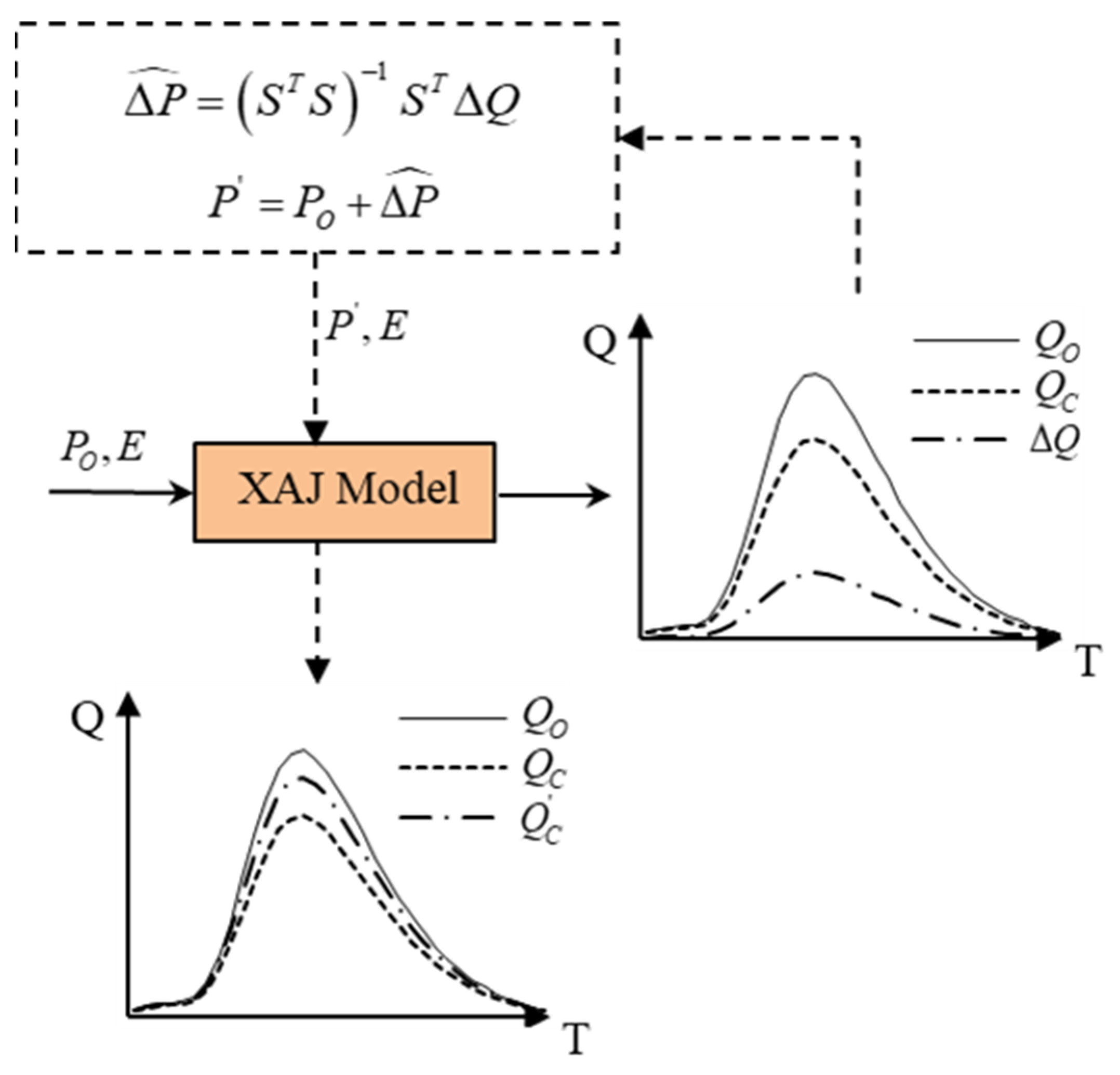
2.1. DSRC Method
2.2. DSRC-R Method
2.3. L-Curve Criterion
2.4. New Optimization Criterion (BSR)
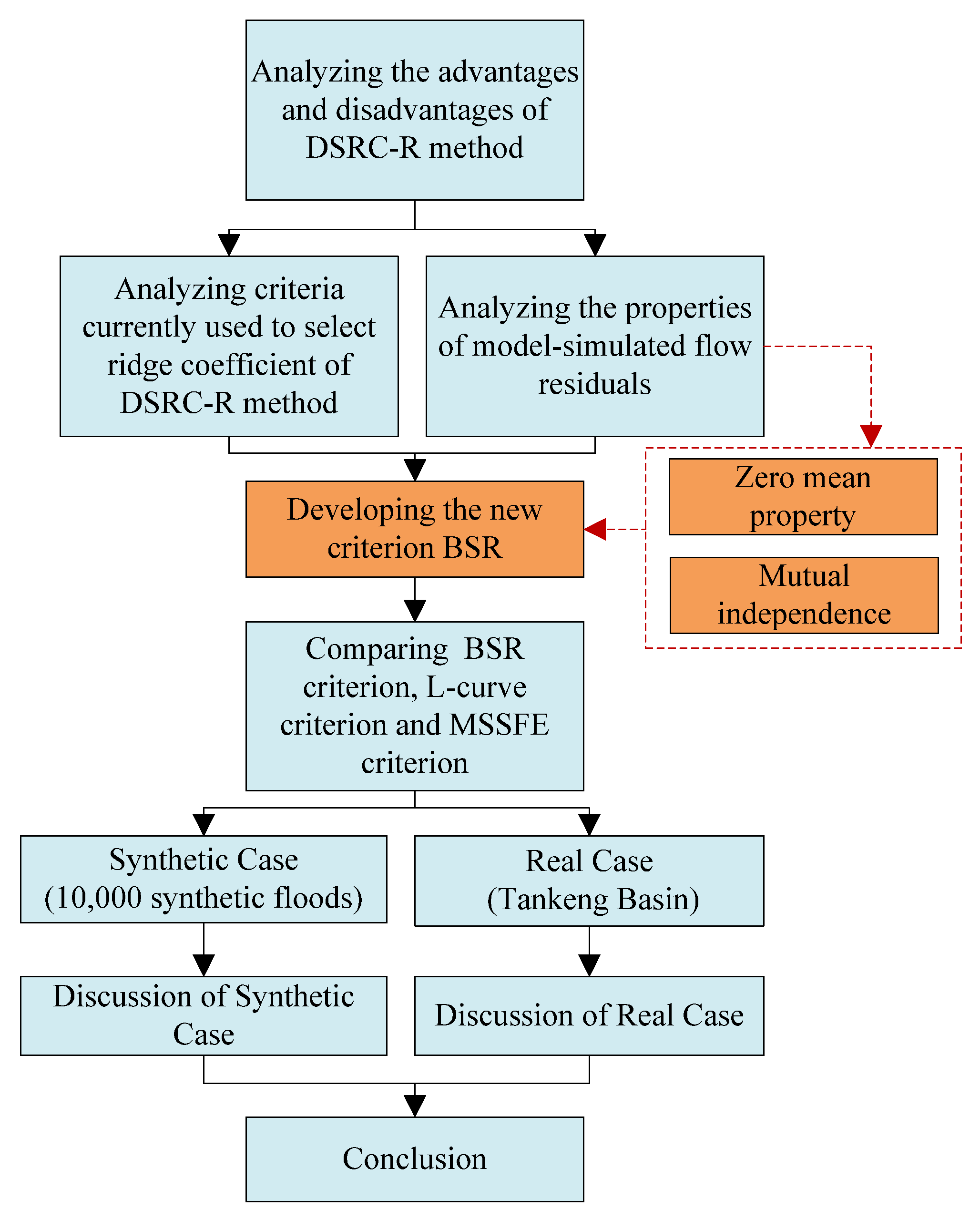
2.5. The Entire Research Process
3. Case Study
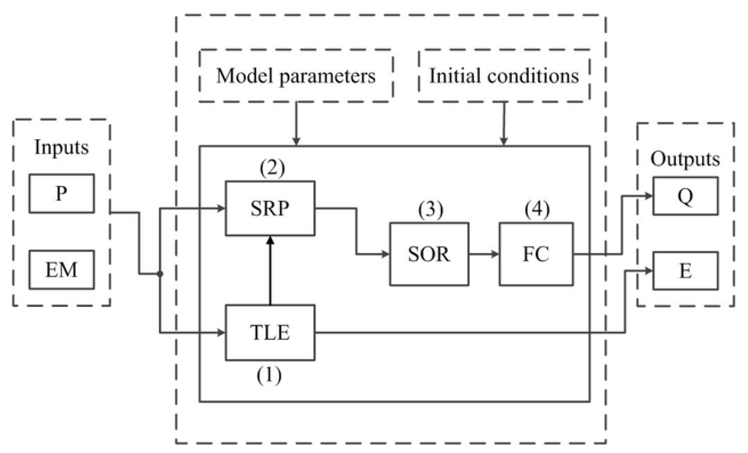
3.1. Model Description
3.2. Synthetic Case
3.2.1. Data
3.2.2. Statistical Indicators
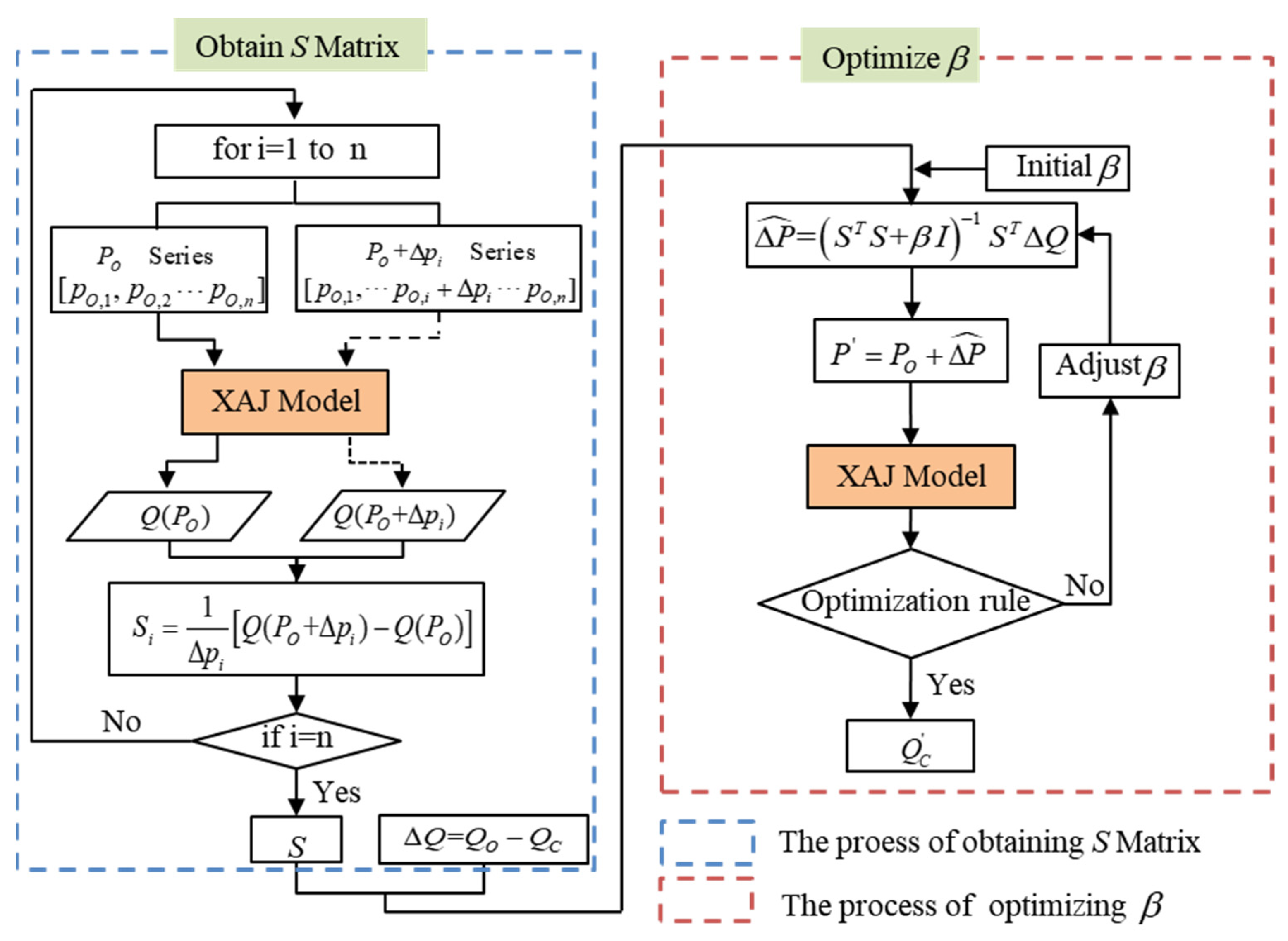
3.2.3. Computational Process of DSRC Method and DSRC-R Method
- Add the additional precipitation in the i-th time interval to the precipitation in the i-th time interval while keeping the precipitation in the j-th time interval () unchanged; then, obtain the new precipitation series .
- Introduce the original precipitation series and new precipitation series into the model and obtain the series and , respectively. Then, is obtained by the equation , where is the dynamic system response curve of the i-th rainfall, that is, the i-th column of matrix S.
- Cycle Steps 1 and 2 n times and obtain the precipitation dynamic system response matrix .
- Add the estimated precipitation error series to the original precipitation series and obtain the updated precipitation series .
- Introduce the updated precipitation series into the model in order to obtain the updated forecasted flow .
- Initialize the ridge coefficient ;
- Obtain the precipitation error estimation series . Add to in order to obtain ;
- Rerun the model with and obtain the updated flow process ;
- Judge whether the results meet the criteria (the criteria adopted in this essay include the BSR criterion, the L-curve criterion and the MSSFE criterion). If yes, turn to Step 6; if no, go back to Step 5;
- Adjust the ridge coefficient according to the optimization algorithm (this essay applied the particle swarm optimization algorithm) and then turn to Step 2;
- Finish the optimization process and acquire the optimal ridge coefficient .
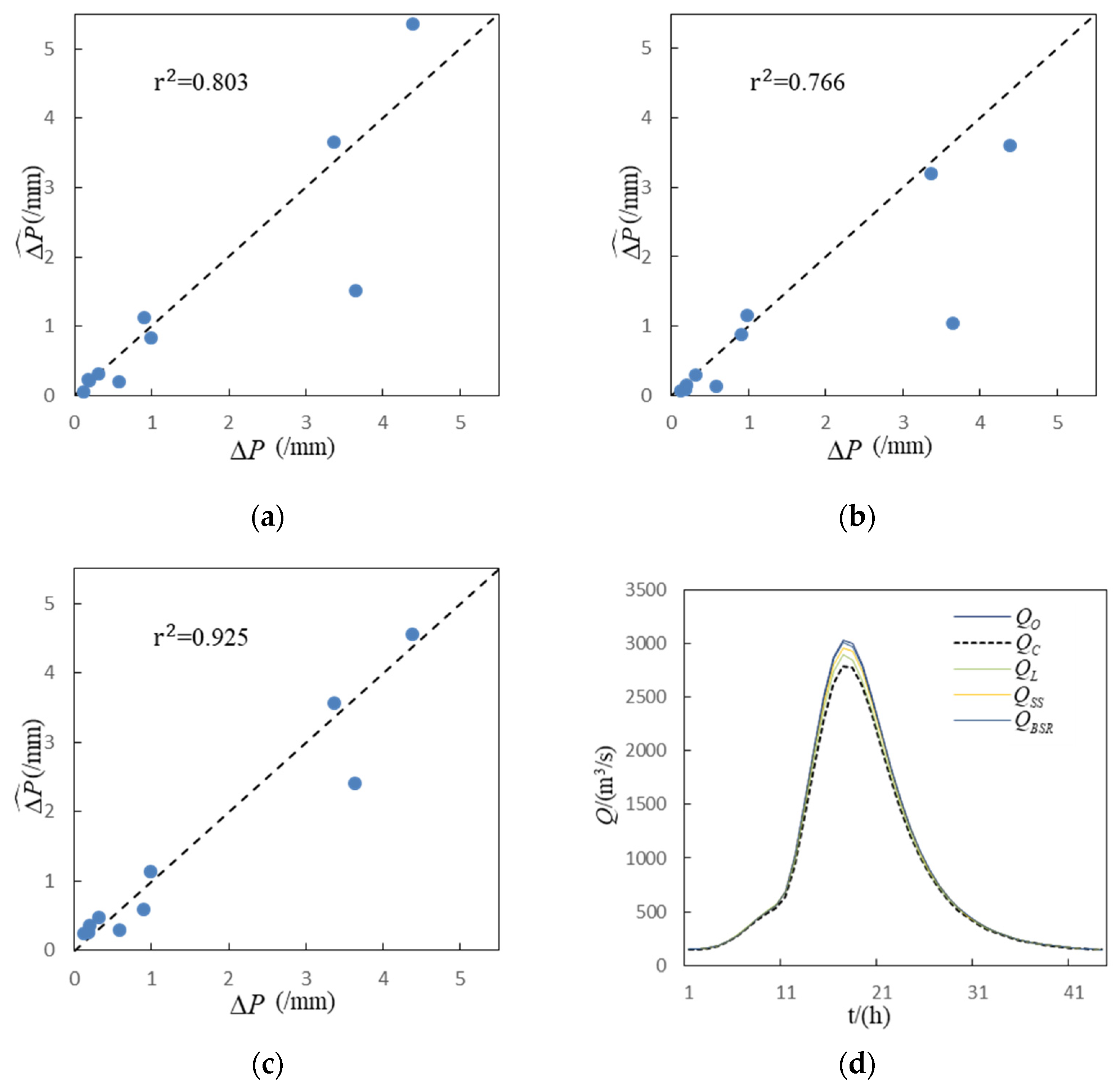
3.2.4. Results and Discussion
3.3. Real Case
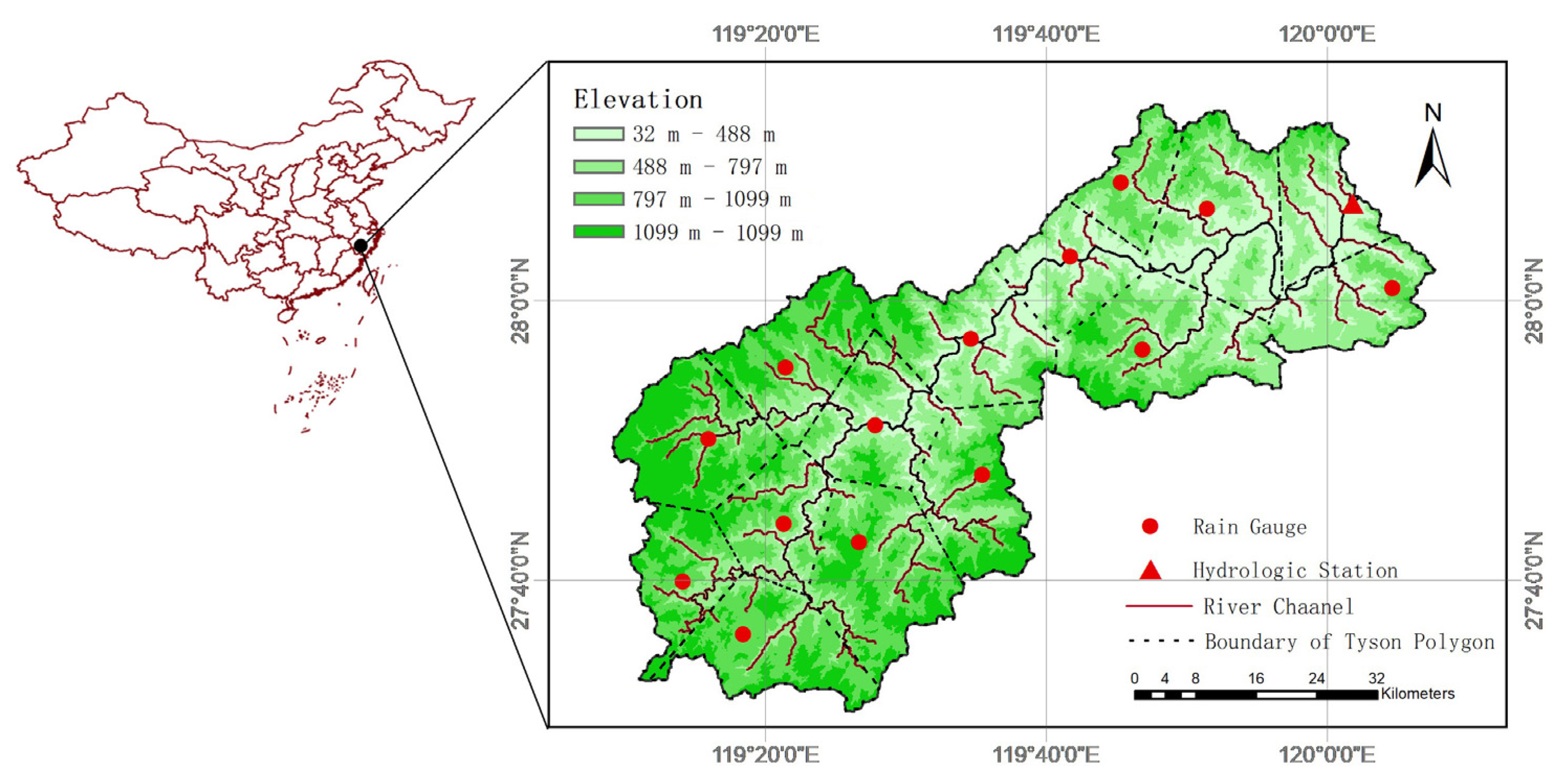
3.3.1. Data
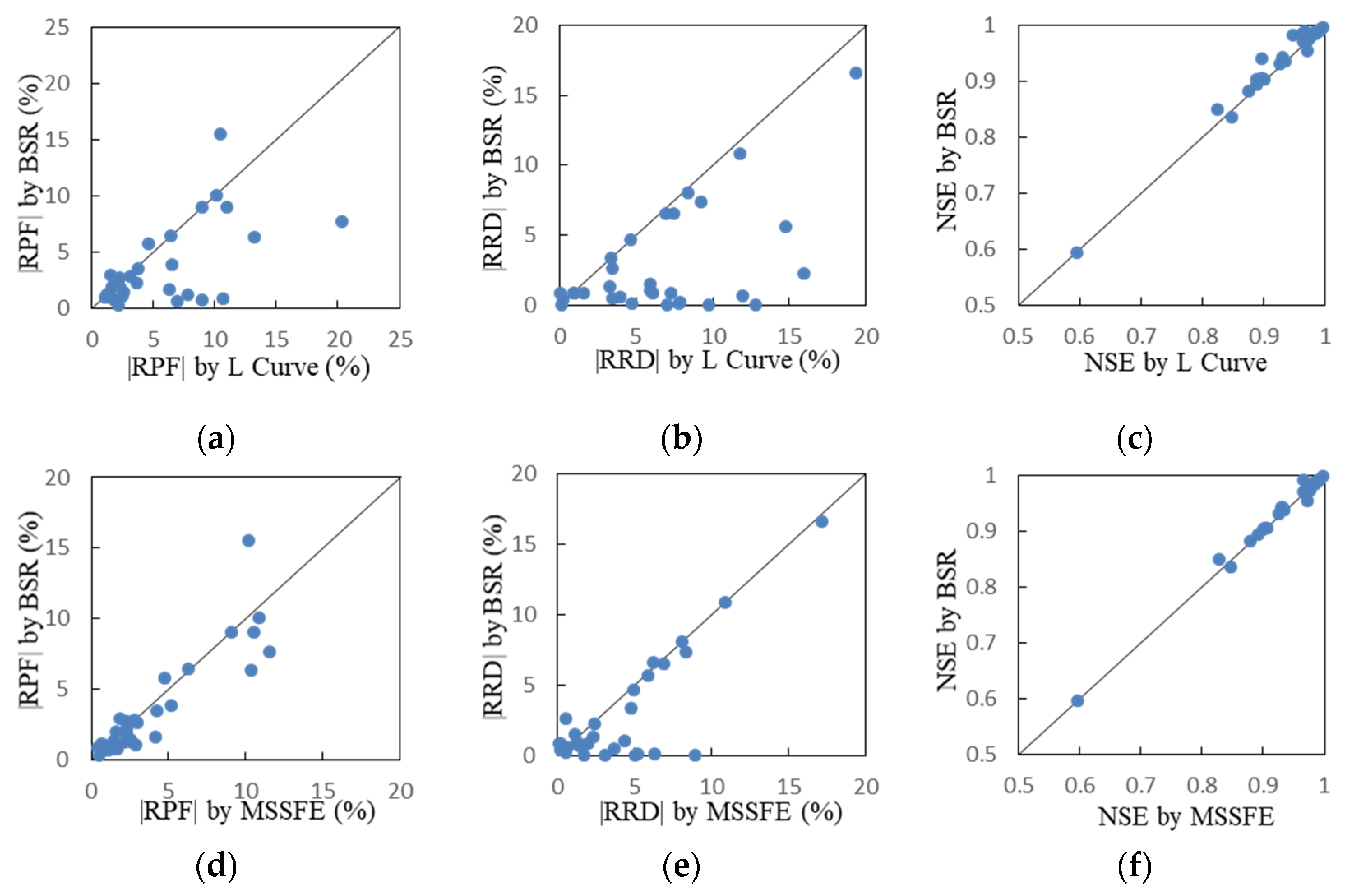
3.3.2. Results and Discussion
4. Conclusions and Prospect
Author Contributions
Funding
Data Availability Statement
Acknowledgments
Conflicts of Interest
Appendix A. Proof of in the DSRC-R Method
Appendix B. Proof of
Appendix C

| Flood Number | Before Updating | L-Curve | MSSFE | BSR | |||||||||||||||||
|---|---|---|---|---|---|---|---|---|---|---|---|---|---|---|---|---|---|---|---|---|---|
| RPF | RRD | NSE | RPF | RRD | NSE | BDSR | RDSR | TU | RPF | RRD | NSE | TU | BDSR | RDSR | RPF | RRD | NSE | TU | BDSR | RDSR | |
| 31850823 | 10.1 | −14.41 | 0.934 | 6.42 | −9.26 | 0.974 | 468.0 | 1.32 | 25.2 | 6.25 | −8.31 | 0.975 | 8.1 | 959.6 | 1.30 | 6.41 | −7.38 | 0.985 | 15.3 | 6.2 | 1.33 |
| 31860520 | 2.77 | −11.18 | 0.743 | 2.56 | 9.71 | 0.972 | 2958.1 | 1.59 | 42.5 | 2.52 | 8.89 | 0.973 | 21.1 | 2718.9 | 1.83 | 1.38 | −0.02 | 0.954 | 18.7 | 2461.2 | 3.25 |
| 31870910 | −11.7 | −7.38 | 0.952 | 8.93 | 3.38 | 0.963 | 1256.9 | 1.06 | 29.4 | −1.72 | −4.77 | 0.986 | 6.4 | 1418.6 | 1.09 | 0.74 | −3.35 | 0.984 | 9.9 | 40.6 | 2.35 |
| 31880520 | −16.44 | −10.91 | 0.762 | 6.93 | 7.49 | 0.888 | 2070.8 | 1.10 | 43.3 | 0.95 | −6.17 | 0.903 | 11.1 | 236.0 | 1.31 | 0.65 | −6.57 | 0.904 | 10.0 | 32.1 | 1.48 |
| 31880922 | −5.48 | −13.33 | 0.755 | −1.19 | 6.99 | 0.976 | 2314.3 | 1.13 | 28.6 | −0.66 | 5.06 | 0.979 | 30.6 | 2530.1 | 1.16 | 1.15 | 0.03 | 0.979 | 35.3 | 149.5 | 1.56 |
| 31890527 | −17.28 | −3.54 | 0.805 | 3.65 | 3.97 | 0.971 | 673.3 | 1.05 | 46.6 | 2.29 | 0.56 | 0.971 | 9.2 | 11.1 | 1.02 | 2.25 | 0.54 | 0.975 | 14.7 | 5.5 | 1.33 |
| 31890618 | −15.11 | −14.14 | 0.753 | 6.26 | 12.78 | 0.966 | 1210.2 | 1.08 | 24.9 | −4.18 | −3.05 | 0.977 | 7.8 | 2479.9 | 1.05 | 1.63 | −0.02 | 0.973 | 8.8 | 2.78 | 1.13 |
| 31890721 | −13.78 | −17.3 | 0.866 | 1.87 | 7.78 | 0.982 | 1387.1 | 1.24 | 32.8 | 1.46 | 6.31 | 0.984 | 10.0 | 1623.5 | 1.26 | 0.76 | −0.12 | 0.986 | 13.3 | 49.0 | 1.35 |
| 31920830 | −13.34 | 9.85 | 0.959 | −1.57 | 6.98 | 0.992 | 1847.3 | 1.40 | 39.3 | −1.82 | 6.88 | 0.992 | 15.5 | 1304.8 | 1.61 | −2.94 | 6.5 | 0.992 | 17.0 | 1161.8 | 1.73 |
| 31940821 | 13.96 | −15.18 | 0.935 | 4.64 | 1.61 | 0.991 | 2249.6 | 1.29 | 17.6 | 4.76 | 1.31 | 0.991 | 9.5 | 1934.0 | 1.33 | 5.76 | −0.82 | 0.99 | 8.5 | 12.5 | 1.37 |
| 31960801 | −17.42 | −1.81 | 0.937 | −2.26 | 0.22 | 0.971 | 4241.8 | 1.99 | 24.3 | −2.31 | 0.2 | 0.971 | 5.4 | 4231.6 | 1.98 | −1.9 | 0.4 | 0.971 | 9.7 | 4344.9 | 2.06 |
| 31970703 | −4.69 | −0.37 | 0.781 | 1.32 | 14.73 | 0.983 | 3240.7 | 1.15 | 29.4 | 2.12 | 5.89 | 0.983 | 8.0 | 3179.3 | 1.16 | 1.2 | 5.64 | 0.983 | 13.5 | 3068.3 | 1.17 |
| 31980618 | −5.91 | 4.28 | 0.96 | 1.43 | 15.92 | 0.997 | 1120.8 | 2.18 | 26.4 | 1.43 | 2.41 | 0.997 | 10.9 | 1127.6 | 2.22 | 1.32 | 2.23 | 0.997 | 7.9 | 1012.9 | 3.78 |
| 31990525 | −18.28 | −8.19 | 0.917 | 10.67 | 7.84 | 0.947 | 400.8 | 1.06 | 31.7 | −0.45 | 0.48 | 0.983 | 8.3 | 135.7 | 1.08 | −0.84 | 0.22 | 0.983 | 7.6 | 2.2 | 1.09 |
| 31990711 | −2.94 | −8.89 | 0.867 | 2.23 | 3.46 | 0.967 | 1430.2 | 1.13 | 24.6 | 2.27 | −0.54 | 0.967 | 9.9 | 1133.0 | 1.14 | 2.71 | −2.64 | 0.99 | 6.4 | 8.3 | 1.14 |
| 31000609 | −20.05 | −7.3 | 0.946 | −8.96 | 0.14 | 0.964 | 671.1 | 1.78 | 32.3 | −10.56 | −1.68 | 0.968 | 12.1 | 663.2 | 1.80 | −9.03 | 0.03 | 0.971 | 10.3 | 623.6 | 1.80 |
| 31000823 | 8.75 | 68.53 | 0.907 | 3.14 | 7.29 | 0.991 | 1621.2 | 1.06 | 26.2 | 2.81 | −1.37 | 0.992 | 15.6 | 990.1 | 1.63 | 2.81 | −0.87 | 0.991 | 8.6 | 967.0 | 1.66 |
| 31030624 | −11.61 | 58.79 | 0.866 | −1.83 | 6.08 | 0.981 | 659.4 | 1.03 | 24.9 | −1.07 | −1.97 | 0.982 | 8.0 | 522.1 | 1.02 | 0.7 | −0.81 | 0.986 | 5.2 | 32.6 | 1.89 |
| 31040812 | 19.29 | 36.59 | 0.84 | 20.29 | 5.93 | 0.896 | 1214.4 | 1.52 | 15.2 | 11.58 | 1.11 | 0.93 | 4.0 | 1203.5 | 1.49 | 7.68 | −1.46 | 0.941 | 6.5 | 1205.4 | 1.53 |
| 31850604 | −13.11 | −17.32 | 0.754 | 6.49 | 3.3 | 0.934 | 573.5 | 1.14 | 11.7 | 5.14 | 2.3 | 0.935 | 5.3 | 443.1 | 1.15 | 3.87 | 1.31 | 0.935 | 6.8 | 4.4 | 1.28 |
| 31850626 | −10.91 | −3.17 | 0.821 | −2.03 | 11.97 | 0.896 | 59.6 | 2.01 | 16.3 | −2.93 | −1.49 | 0.906 | 10.5 | 388.3 | 1.08 | −2.61 | −0.7 | 0.905 | 9.7 | 22.9 | 2.12 |
| 31860330 | −27.8 | −18.3 | 0.68 | 3.71 | 0.96 | 0.968 | 28.7 | 1.15 | 38.7 | 4.23 | 1.23 | 0.969 | 36.9 | 112.8 | 1.14 | 3.47 | 0.86 | 0.968 | 33.0 | 8.7 | 1.15 |
| 31860428 | 41.36 | 19.54 | 0.02 | 10.92 | 11.8 | 0.825 | 1488.3 | 1.09 | 19.7 | 9.04 | 10.89 | 0.828 | 6.8 | 517.8 | 1.32 | 9.02 | 10.87 | 0.849 | 5.9 | 515.1 | 1.32 |
| 31870411 | −2.08 | −6.7 | 0.724 | 13.18 | 5.89 | 0.875 | 2131.9 | 1.29 | 14.5 | 10.36 | 4.31 | 0.879 | 5.4 | 1975.7 | 1.22 | 6.34 | 0.99 | 0.879 | 14.1 | 1806.3 | 1.37 |
| 31870527 | −23.87 | −9.43 | 0.738 | −10.41 | 3.49 | 0.847 | 298.6 | 1.19 | 16.3 | −10.2 | 3.62 | 0.847 | 9.7 | 225.3 | 1.20 | −15.5 | 0.5 | 0.836 | 16.8 | 225.1 | 1.20 |
| 31880327 | −19.21 | −6.61 | 0.869 | −10.11 | −4.66 | 0.901 | 404.8 | 1.02 | 24.8 | −10.87 | −4.94 | 0.901 | 7.6 | 168.0 | 1.06 | −10.08 | −4.65 | 0.903 | 8.5 | 8.36 | 1.06 |
| 31880524 | 8.66 | −2.92 | 0.429 | 1.59 | 0.09 | 0.926 | 50.4 | 1.03 | 19.9 | 1.61 | 0.1 | 0.926 | 10.3 | 23.3 | 1.05 | −1.94 | −0.83 | 0.931 | 6.4 | 4.1 | 1.21 |
| 31880613 | −29.34 | −10.44 | 0.193 | 1.07 | 0.91 | 0.595 | 353.5 | 1.23 | 16.1 | −0.91 | −0.15 | 0.597 | 9.0 | 431.7 | 1.20 | 0.91 | 0.82 | 0.595 | 5.3 | 4.8 | 1.24 |
| 31880627 | 0.97 | 47.39 | 0.412 | 2.51 | 4.76 | 0.967 | 876.5 | 1.17 | 18.4 | 2.84 | 5.15 | 0.967 | 5.3 | 411.9 | 2.04 | −1.09 | −0.07 | 0.971 | 17.0 | 480.5 | 2.70 |
| 31890413 | 14.65 | 10.1 | 0.125 | 2.18 | 8.35 | 0.931 | 617.2 | 1.03 | 20.8 | 0.54 | 8.11 | 0.932 | 3.8 | 516.5 | 1.07 | 0.27 | 8.07 | 0.932 | 8.6 | 492.5 | 2.16 |
| 31980513 | 28.8 | 57.29 | 0.098 | 7.8 | 19.32 | 0.889 | 1438.5 | 1.03 | 13.8 | 2.63 | 17.14 | 0.892 | 8.1 | 1312.3 | 1.65 | 1.25 | 16.6 | 0.893 | 16.2 | 1332.4 | 2.58 |
| Average 1 | 14.51 | 16.81 | 0.721 | 5.42 | 6.68 | 0.933 | 1269.6 | 1.28 | 25.7 | 3.95 | 4.08 | 0.938 | 10.7 | 1126.7 | 1.34 | 3.49 | 2.77 | 0.940 | 12.1 | 648.1 | 1.69 |
References
- Wang, Y.; Liu, R.; Guo, L.; Tian, J.; Zhang, X.; Ding, L.; Wang, C.; Shang, Y. Forecasting and providing warnings of flash floods for ungauged mountainous areas based on a distributed hydrological model. Water 2017, 9, 776. [Google Scholar] [CrossRef] [Green Version]
- Cheng, W.; Huang, C.; Hsu, N.; Wei, C. Risk Analysis of Reservoir Operations Considering Short-Term Flood Control and Long-Term Water Supply: A Case Study for the Da-Han Creek Basin in Taiwan. Water 2017, 9, 424. [Google Scholar] [CrossRef] [Green Version]
- Bao, W.; Si, W.; Shen, G.; Zhang, X.; Li, Q. Runoff error updating based on unit hydrograph inversion. Adv. Water Sci. 2012, 23, 315–322. [Google Scholar]
- Abrahart, R.J.; See, L. Comparing neural network and autoregressive moving average techniques for the provision of continuous river flow forecasts in two contrasting catchments. Hydrol. Process. 2000, 14, 2157–2172. [Google Scholar] [CrossRef]
- Broersen, P.M.; Weerts, A.H. Automatic Error Correction of Rainfall-Runoff models in Flood Forecasting Systems. IMTC IEEE 2005, 6, 963–968. [Google Scholar]
- Bogner, K.; Pappenberger, F. Multiscale error analysis, correction, and predictive uncertainty estimation in a flood forecasting system. Water Resour. Res. 2011, 47, 1772–1780. [Google Scholar] [CrossRef] [Green Version]
- Sun, L.; Nistor, I.; Seidou, O. Streamflow data assimilation in SWAT model using Extended Kalman Filter. J. Hydrol. 2015, 531, 671–684. [Google Scholar] [CrossRef]
- Moradkhani, H.; Gupta, H.; Sorooshian, S.V.; Houser, P. Combined parameter and state estimation of hydrological models using ensemble Kalman filter. Adv. Water Resour. 2005, 28, 135–147. [Google Scholar] [CrossRef] [Green Version]
- Wagener, T.; Mcintyre, N.; Lees, M.J.; Wheater, H.S.; Gupta, H.V. Towards reduced uncertainty in conceptual rainfall-runoff modelling: Dynamic identifiability analysis. Hydrol. Process. 2003, 17, 455–476. [Google Scholar] [CrossRef]
- Misirli, F.; Gupta, H.V.; Sorooshian, S.; Thiemann, M. Bayesian Recursive Estimation of Parameter and Output Uncertainty for Watershed Models; American Geophysical Union (AGU): Washington, DC, USA, 2013. [Google Scholar]
- Bao, W.; Ji, H.; Hu, Q.; Qu, S.; Zhao, C. Robust estimation theory and its application to hydrology. Adv. Water Sci. 2003, 14, 528–532. [Google Scholar]
- Qu, S.; Bao, W. Comprehensive correction of real-time flood forecasting. Adv. Water Sci. 2003, 14, 167–171. [Google Scholar]
- Dechant, C.M.; Moradkhani, H. Examining the effectiveness and robustness of sequential data assimilation methods for quantification of uncertainty in hydrologic forecasting. Water Resour. Res. 2012, 48, W04518. [Google Scholar] [CrossRef] [Green Version]
- Bao, W.; Si, W.; Qu, S. Flow Updating in Real-Time Flood Forecasting Based on Runoff Correction by a Dynamic System Response Curve. J. Hydrol. Eng. 2014, 19, 747–756. [Google Scholar]
- Si, W.; Bao, W.; Qu, S. Runoff error correction in real-time flood forecasting based on dynamic system response curve. Adv. Water Sci. 2013, 24, 497–503. [Google Scholar]
- Si, W.; Bao, W.; Gupta, H.V. Updating real-time flood forecasts via the dynamic system response curve method. Water Resour. Res. 2015, 51, 5128–5144. [Google Scholar] [CrossRef]
- Sun, Y.; Bao, W.; Jiang, P.; Si, W.; Zhou, J.; Zhang, Q. Development of a Regularized Dynamic System Response Curve for Real-Time Flood Forecasting Correction. Water 2018, 10, 450. [Google Scholar] [CrossRef] [Green Version]
- Sun, Y.; Bao, W.; Jiang, P.; Ji, X.; Gao, S.; Xu, Y.; Si, W. Development of Multivariable Dynamic System Response Curve Method for Real-Time Flood Forecasting Correction. Water Resour. Res. 2018, 54, 4730–4749. [Google Scholar] [CrossRef]
- Si, W.; Gupta, H.V.; Bao, W.; Jiang, P.; Wang, W. Improved Dynamic System Response Curve Method for Real-Time Flood Forecast Updating. Water Resour. Res. 2019, 55, 7493–7519. [Google Scholar] [CrossRef] [Green Version]
- Liu, K.; Zhang, X.; Bao, W.; Zhao, L.; Shu, H.; Li, J. A system response correction method with runoff error smooth matrix. J. Hydraul. Eng. 2015, 46, 960–966. [Google Scholar]
- Hansen, P.C.; Oleary, D.P. The use of the L-curve in the regularization of discrete ill-posed problems. SIAM J. Sci. Comput. 1993, 14, 1487–1503. [Google Scholar] [CrossRef]
- Zhao, R.J. The Xinanjiang model applied in China. J. Hydrol. 1992, 135, 371–381. [Google Scholar]
- Hansen, P.C. Analysis of discrete ill-posed problems by means of the L-curve. SIAM Rev. 1992, 34, 561–580. [Google Scholar] [CrossRef]
- Kennedy, J.; Eberhart, R.C. Particle swarm optimization. In Proceedings of the International Conference on Neural Networks, Perth, Australia, 27 November–1 December 1995. [Google Scholar]
- Sierra, M.R.; Coello, C.A. Improving PSO-Based Multi-objective Optimization Using Crowding, Mutation and E-Dominance. Lect. Notes Comput. Sc. 2005, 3410, 505–519. [Google Scholar]
- Mesloub, S.; Mansour, A. Hybrid PSO and GA for global maximization. Int. J. Comput. Math 2009, 2, 597–608. [Google Scholar]
- Chen, Y.; Li, J.; Xu, H. Improving flood forecasting capability of physically based distributed, hydrological models by parameter optimization. Hydrol. Earth Syst. Sci. 2016, 20, 375–392. [Google Scholar] [CrossRef] [Green Version]
- Zhang, X.; Liu, K.; Bao, W.; Li, J.; Lai, S. Runoff error proportionality coefficient correction method based on system response. Adv. Water Sci. 2014, 25, 789–796. [Google Scholar]


| Layer | Function | Parameter | Meaning |
|---|---|---|---|
| First layer | Evaporation | K | Ratio of potential evapotranspiration to pan evaporation |
| WUM | Areal mean tension water capacity of the upper layer | ||
| WLM | Areal mean tension water capacity of the lower layer | ||
| WDM | Areal mean tension water capacity of the deeper layer | ||
| C | Coefficient of deep evapotranspiration | ||
| Second layer | Runoff production | IM | Ratio of impervious area |
| WM | Areal mean tension water capacity | ||
| B | Exponent of the tension water capacity distribution curve | ||
| Third layer | Runoff separation | SM | Areal mean free water capacity of the surface soil layer |
| EX | Exponent of the free water capacity curve | ||
| KI | Outflow coefficients of the free water storage to interflow | ||
| KG | Outflow coefficients of the free water storage to groundwater | ||
| Fourth layer | Flow Concentration | CS | Recession constant of the surface water storage |
| CI | Recession constant of the interflow storage | ||
| CG | Recession constant of the groundwater storage | ||
| KE | Storage time constant | ||
| XE | Weight factor |
| Parameter | K | WM | WUM | WLM | WDM | IM | B | C | SM |
|---|---|---|---|---|---|---|---|---|---|
| Value | 1.1 | 150 | 20 | 80 | 50 | 0.01 | 0.3 | 0.16 | 10 |
| Parameter | EX | KI | KG | CS | CI | CG | KE | XE | |
| Value | 1.5 | 0.35 | 0.35 | 0.78 | 0.865 | 0.995 | 1.50 | 0.380 |
| Items 1 | RPF | RRD | NSE | RDSR | BDSR | TU | RMSE | |
|---|---|---|---|---|---|---|---|---|
| Before correction | 9.38 | 5.12 | 0.985 | —— | —— | —— | —— | —— |
| L-curve | 2.19 | 1.30 | 0.998 | 5.57 | 80.8 | 12.21 | 985.11 | 0.941 |
| MSSFE | 1.97 | 1.27 | 0.999 | 9.31 | 74.8 | 3.99 | 64.26 | 1.040 |
| BSR | 1.90 | 1.01 | 0.999 | 12.88 | 66.9 | 4.11 | 821.35 | 0.759 |
| Parameter | K | WM | WUM | WLM | WDM | IM | B | C | SM | EX |
|---|---|---|---|---|---|---|---|---|---|---|
| Value | 1.296 | 150 | 20 | 80 | 50 | 0.01 | 0.3 | 0.16 | 10 | 1.5 |
| Parameter | KI | KG | CS | CI | CG | KE | XE | |||
| Value | 0.35 | 0.35 | 0.65 | 0.865 | 0.95 | 1.466 | 0.380 |
Publisher’s Note: MDPI stays neutral with regard to jurisdictional claims in published maps and institutional affiliations. |
© 2021 by the authors. Licensee MDPI, Basel, Switzerland. This article is an open access article distributed under the terms and conditions of the Creative Commons Attribution (CC BY) license (https://creativecommons.org/licenses/by/4.0/).
Share and Cite
Liu, K.; Bao, W.; Hu, Y.; Sun, Y.; Li, D.; Li, K.; Liang, L. Improvement in Ridge Coefficient Optimization Criterion for Ridge Estimation-Based Dynamic System Response Curve Method in Flood Forecasting. Water 2021, 13, 3483. https://doi.org/10.3390/w13243483
Liu K, Bao W, Hu Y, Sun Y, Li D, Li K, Liang L. Improvement in Ridge Coefficient Optimization Criterion for Ridge Estimation-Based Dynamic System Response Curve Method in Flood Forecasting. Water. 2021; 13(24):3483. https://doi.org/10.3390/w13243483
Chicago/Turabian StyleLiu, Kexin, Weimin Bao, Yufeng Hu, Yiqun Sun, Dongjing Li, Kuang Li, and Lili Liang. 2021. "Improvement in Ridge Coefficient Optimization Criterion for Ridge Estimation-Based Dynamic System Response Curve Method in Flood Forecasting" Water 13, no. 24: 3483. https://doi.org/10.3390/w13243483