Development of Boosted Machine Learning Models for Estimating Daily Reference Evapotranspiration and Comparison with Empirical Approaches

Abstract

Proper irrigation scheduling and agricultural water management require a precise estimation of crop water requirement. In practice, reference evapotranspiration (ETo) is firstly estimated, and used further to calculate the evapotranspiration of each crop. In this study, two new coupled models were developed for estimating daily ETo. Two optimization algorithms, the shuffled frog-leaping algorithm (SFLA) and invasive weed optimization (IWO), were coupled on an adaptive neuro-fuzzy inference system (ANFIS) to develop and implement the two novel hybrid models (ANFIS-SFLA and ANFIS-IWO). Additionally, four empirical models with varying complexities, including Hargreaves–Samani, Romanenko, Priestley–Taylor, and Valiantzas, were used and compared with the developed hybrid models. The performance of all investigated models was evaluated using the ETo estimates with the FAO-56 recommended method as a benchmark, as well as multiple statistical indicators including root-mean-square error (RMSE), relative RMSE (RRMSE), mean absolute error (MAE), coefficient of determination (R²), and Nash–Sutcliffe efficiency (NSE). All models were tested in Tabriz and Shiraz, Iran as the two studied sites. Evaluation results showed that the developed coupled models yielded better results than the classic ANFIS, with the ANFIS-SFLA outperforming the ANFIS-IWO. Among empirical models, generally the Valiantzas model in its original and calibrated versions presented the best performance. In terms of model complexity (the number of predictors), the model performance was obviously enhanced by an increasing number of predictors. The most accurate estimates of the daily ETo for the study sites were achieved via the hybrid ANFIS-SFLA models using full predictors, with RMSE within 0.15 mm day⁻¹, RRMSE within 4%, MAE within 0.11 mm day⁻¹, and both a high R² and NSE of 0.99 in the test phase at the two studied sites.

1. Introduction

Evapotranspiration (ET) is an important component of the hydrologic cycle. An accurate estimation of ET is required for many applications, such as optimal water resources management, irrigation planning, determination of irrigation intervals, design of irrigation systems, agricultural water management, and studies related to water balance at each area [1,2,3,4,5,6]. Lysimeters are commonly applied to directly measure the ET; however, measuring it with this method is costly and requires considerable time, making it difficult to use in many areas. Additionally, eddy covariance and Bowen ratio energy balance are other direct techniques of determining the ET that are not usually applied in practice due to their complexities and costs [7,8,9]. Hence, indirect techniques are often used to estimate ET. One of these indirect methods is the use of empirical models that can be classified into several groups, including temperature-based, radiation-based, and mass-transfer-based models, etc. In all empirical models, reference evapotranspiration (ETo) is estimated. The reason is that estimating ET for each crop is difficult. Therefore, ETo is firstly estimated via the indirect methods, and crop coefficients are then used for estimating the ET of any desired crop. The Food and Agricultural Organization (FAO) has recommended the Penman–Monteith method (i.e., FAO-56 PM) as a benchmark for obtaining the ETo [10]. The ETo process seems to be a complex and nonlinear phenomenon due to its dependence on a variety of weather data comprising the air temperature, relative humidity, wind speed, radiation, etc. [11,12]. In addition to the empirical models, machine learning (ML) approaches have recently received remarkable attention in modeling the ETo, and have shown reasonable performances. The ML techniques are capable of capturing hydrological time series such as ETo by utilizing solely a series of predictors without any knowledge of their physical processes [13,14,15].

Numerous studies have been reported in recent years on ETo modeling via ML approaches. Torres et al. [16] used a multivariate relevance vector machine (MVRVM) and a multilayer perceptron (MLP) for the daily ETo modeling of an experimental site in central Utah, USA. The effectiveness and suitability of the applied models were reported. The daily ETo of Dar El Beid, Algeria, was modeled by generalized regression neural networks (GRNN) and radial basis function neural networks (RBFNN) [17]. The GRNN outperformed the RBFNN and two empirical models used. Kisi and Cengiz [18] applied a fuzzy genetic (FG) algorithm and an artificial neural network (ANN) in daily ETo forecasting for Antalya and Isparta, Turkey. The FG was found to provide higher accuracy compared to the ANN. An extreme learning machine (ELM) was implemented by Abdullah et al. [19] for predicting the monthly mean ETo in three locations in Iraq. The ELM demonstrated superior results compared to feed-forward back-propagation (FFBP). Wen et al. [20] estimated the daily ETo of an extremely arid region in China via an ANN, a support vector machine (SVM), and three empirical models. The SVM was reported as the best-performing model. A performance evaluation of gene expression programming (GEP) and an ANN was conducted by Wang et al. [21] for modeling daily ETo in four locations in China. The ANN showed superiority over the GEP. Traore et al. [22] applied four types of ANNs for predicting the ETo at a weather station in Texas, USA, and found that the MLP performed the best. Mehdizadeh [23] developed hybrid models using antecedent data of ETo for the daily ETo forecasting of six stations in Iran through hybridizing multivariate adaptive regression splines (MARS) and GEP with a nonlinear time series model, called auto-regressive conditional heteroscedasticity (ARCH). The results illustrated the higher accuracy of the coupled models compared to the single ones. Mattar [24] assessed the applicability of GEP for modeling monthly ETo at 32 weather stations in Egypt, and they found that a better modeling performance of the GEP over the empirical models. Sanikhani et al. [25] evaluated the accuracy of ML techniques, including the MLP, GRNN, RBFNN, and two versions of an adaptive neuro-fuzzy inference system (ANFIS); i.e., grid partitioning (ANFIS-GP) and subtractive clustering (ANFIS-SC), to predict the monthly ETo of Antalya and Isparta, Turkey. They developed the ML approaches under temperature-based scenarios, and the accuracy of these ML models was compared to an empirical equation, namely the Hargreaves–Samani. The GEP and GRNN at Antalya, and the RBFNN and ANFIS-SC at Isparta, showed superior results. Saggi and Jain [26] used deep learning (DL) to forecast daily ETo in Punjab, India. It was found that the DL model performed the best when comparing its performance to random forests (RF), generalized linear model (GLM), and gradient boosting machine (GBM).

Recently, bio-inspired optimization algorithms have successfully been hybridized with ML models to improve ETo forecasts. Ozkan et al. [27] proposed a coupled model by hybridizing an artificial bee colony (ABC) and an ANN (i.e., ANN-ABC) for predicting the daily ETo at two stations in the USA. The developed hybrid model outperformed the single ANN. A hybrid ANN–genetic algorithm (i.e., ANN-GA) was implemented by Eslamian et al. [28] for estimating the monthly ETo of selected stations in Isfahan, Central Iran. The monthly ETo estimates of the hybrid ANN-GA were closer to the FAO-56 PM data, compared to the ANN. Yin et al. [29] investigated the accuracy of a developed hybrid SVM-GA, as well as single SVM and feed-forward neural networks (FFNNs), in daily ETo modeling of a semiarid region in China. It was concluded that the hybrid SVM-GA had a better accuracy than the ANN and SVM. A hybrid model was proposed by Tao et al. [30] via combining a firefly algorithm (FA) with ANFIS for estimating daily ETo of three stations located in Burkina Faso. The proposed coupled ANFIS-FA was found to outperform the classic ANFIS. In another work, Wu et al. [31] integrated bio-inspired optimization algorithms, including the GA, ant colony optimization (ACO), cuckoo search algorithm (CSA), and flower pollination algorithm (FPA), with an ELM for forecasting of the daily ETo at eight locations in China. The ELM coupled with the FPA (i.e., ELM-FPA) outperformed the other hybrid models that were developed. Other types of coupled models developed via hybridizing the ML and optimization algorithms have been recently proposed to improve ETo modeling. For example, interested readers can refer to Ahmadi et al. [13], Roy et al. [32], Chia et al. [33], Yan et al. [34], Gong et al. [35], Gao et al. [36], and Dong et al. [37].

Considering the importance of ETo in the optimal agricultural water management and planning for available water resources systems, estimating its values in each region via the suitable approaches is an essential requirement. This study attempted to propose novel models for daily ETo modeling. In this context, two types of optimization algorithms, consisting of the shuffled frog-leaping algorithm (SFLA) and invasive weed optimization (IWO), were coupled on an adaptive neuro-fuzzy inference system (ANFIS) as predictor tools, which was the novelty of this study. Therefore, the coupled ANFIS-SFLA and ANFIS-IWO models were proposed. Additionally, four empirical models, including Hargreaves–Samani, Romanenko, Priestley–Taylor, and Valiantzas, were utilized in both their original and calibrated forms. The performances of the applied models (i.e., the classic ANFIS, the hybrid ANFIS-SFLA and ANFIS-IWO, and original and calibrated forms of the empirical models) were compared with each other by means of multiple error indicators. We focused on two stations in Iran (i.e., Tabriz and Shiraz) as the study sites. To the best of our knowledge, this is the first attempt in the literature to develop a hybrid ANFIS-SFLA and ANFIS-IWO for modeling daily ETo.

2. Materials and Methods

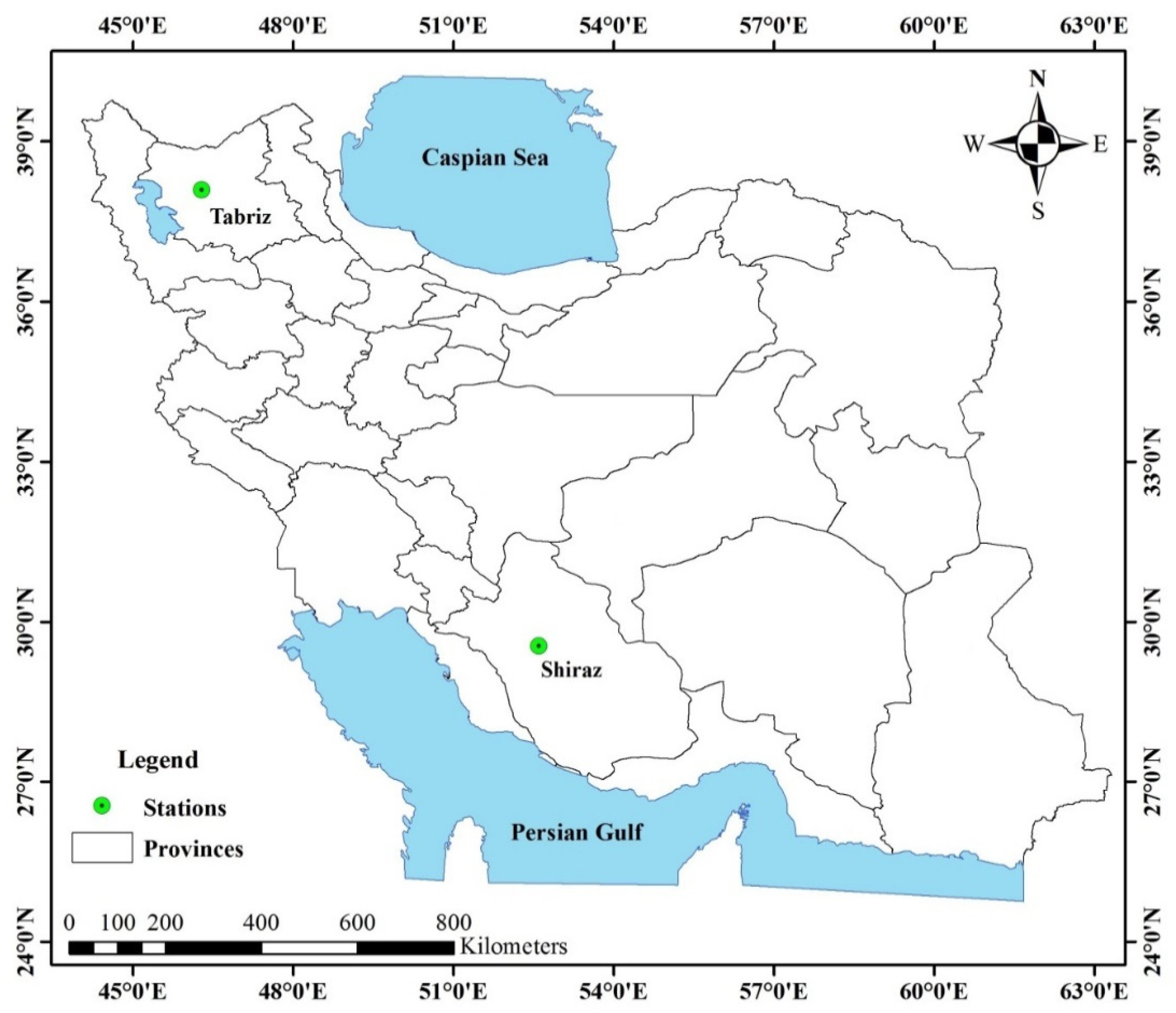
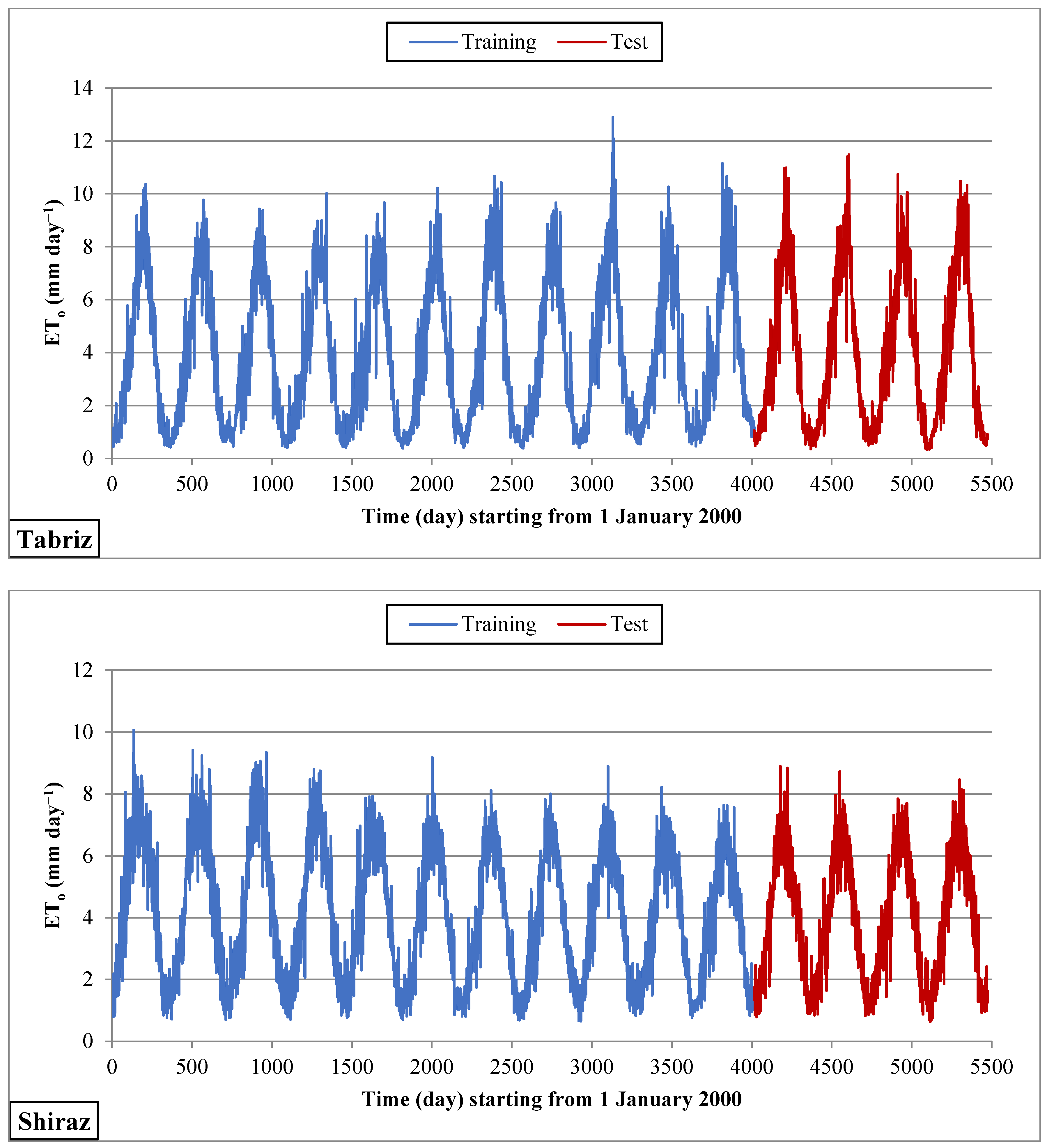
2.1. Study Sites and Data Used

This study considered two sites in Iran, namely Tabriz and Shiraz, as the study locations. The Tabriz station is located in the northwest of Iran, and its latitude, longitude, and altitude are 38°05′ N, 46°17′ E, and 1361.0 m, respectively. The long-term mean annual precipitation at this location is 283.6 mm. In addition, the Shiraz station in the south of Iran is located at a latitude of 29°32′ N, longitude of 52°36′ E, and altitude of 1484 m. The mean annual precipitation of Shiraz is 328.0 mm. The location of the studied sites is shown in Figure 1.

The meteorological data of the study sites, including the minimum temperature (Tmin), maximum temperature (Tmax), average temperature (T), relative humidity (RH), wind speed at 2 m height (U2), solar radiation (Rs), and sunshine duration (SSD) were gathered from the Iran Meteorological Organization (IMO) on a daily time scale over a 15-year period (i.e., 2000–2014). Data from the first 11 years (i.e., 2000–2010) and the last 4 years (i.e., 2011–2014) data were utilized as the training and test datasets, respectively. The daily statistical parameters of the aforementioned data for both training and test phases are tabulated in

Table 1. Statistical characteristics of the data used in this study.

Stations	Parameters	Training					Test
		Xmin	Xmax	Xmean	Xst. dev.	Xcv	Xmin	Xmax	Xmean	Xst. dev.	Xcv
Tabriz	Tmin, °C	−16.80	27.60	8.10	9.38	1.16	−18.00	28.20	7.69	9.67	1.26
	Tmax, °C	−7.90	41.00	19.50	11.18	0.57	−6.80	41.00	19.29	11.49	0.60
	T, °C	−11.85	34.30	13.80	10.19	0.74	−11.80	34.10	13.49	10.47	0.78
	RH, %	10.00	95.00	49.57	16.51	0.33	15.00	91.50	51.41	16.93	0.33
	SSD, h	0.00	13.50	7.85	3.80	0.48	0.00	13.50	7.87	3.85	0.49
	U2, m s−1	0.00	8.31	2.60	1.17	0.45	0.00	8.02	2.77	1.28	0.46
	Rs, MJ m−2 day−1	0.43	33.78	15.18	7.38	0.49	1.09	32.19	18.00	8.40	0.47
	Rn, MJ m−2 day−1	0.74	15.86	7.92	4.55	0.57	1.24	16.36	8.06	4.53	0.56
	Ra, MJ m−2 day−1	14.71	41.82	28.93	9.66	0.33	14.71	41.82	28.93	9.66	0.33
	es-ea, KPa	0.03	4.38	1.15	0.91	0.79	0.05	4.42	1.12	0.93	0.83
	ETo, mm day−1	0.39	12.87	3.88	2.64	0.68	0.34	11.48	3.97	2.81	0.71
Shiraz	Tmin, °C	−7.40	27.20	10.76	7.89	0.73	−8.10	26.40	9.94	7.84	0.79
	Tmax, °C	3.40	42.60	26.64	9.46	0.35	3.40	41.80	26.27	9.64	0.37
	T, °C	−1.00	33.60	18.70	8.50	0.45	−0.80	33.50	18.10	8.55	0.47
	RH, %	12.00	98.50	40.06	16.42	0.41	10.50	96.50	40.21	17.06	0.42
	SSD, h	0.00	12.90	9.33	2.94	0.31	0.00	12.80	9.22	2.86	0.31
	U2, m s−1	0.00	10.25	1.45	0.85	0.59	0.00	4.49	1.36	0.71	0.52
	Rs, MJ m−2 day−1	1.99	31.28	20.21	6.54	0.32	4.94	29.55	20.31	6.16	0.30
	Rn, MJ m−2 day−1	3.10	15.53	9.22	3.65	0.40	3.15	14.92	9.10	3.52	0.39
	Ra, MJ m−2 day−1	19.98	41.13	31.63	7.56	0.24	19.98	41.13	31.63	7.56	0.24
	es-ea, KPa	0.02	4.32	1.70	1.06	0.63	0.03	4.25	1.66	1.08	0.65
	ETo, mm day−1	0.65	10.07	4.12	2.13	0.52	0.62	8.90	3.96	2.03	0.51

. Other parameters in Table 1 comprising Rn (net radiation), Ra (extraterrestrial radiation), saturation vapor pressure deficit (e_s-e_a), and ETo were computed based on the FAO-56 recommended method by Allen et al. [10]. In this table, Xmin, Xmax, Xmean, Xst. dev, and Xcv mean the minimum, maximum, mean, standard deviation, and coefficient of variation of the data used, respectively. As seen, the ETo of Tabriz station ranged from 0.39 mm day⁻¹ to 12.87 mm day⁻¹ (training period) and 0.34 mm day⁻¹ to 11.48 mm day⁻¹ (test period); and between 0.65 mm day⁻¹ and 10.07 mm day⁻¹ (training period) and 0.62 mm day⁻¹ and 8.90 mm day⁻¹ (test period) at the Shiraz station. The lowest values of Xst. dev. in Table 1 for the studied locations were related to U2, e_s-e_a, and ETo; while Ra illustrated the minimal Xcv. Figure 2 shows the time series of daily ETo computed via the FAO-56 PM method for the studied time period (i.e., 2000–2014) at the study sites.

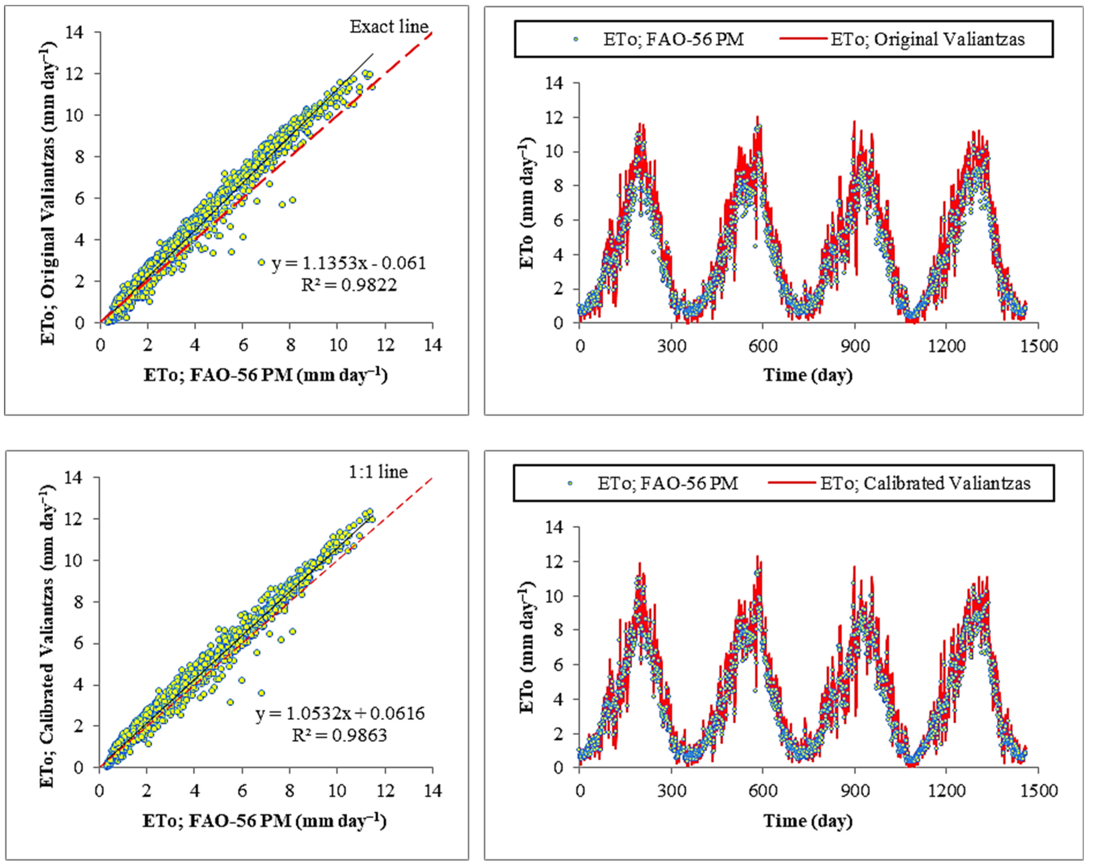
2.2. Empirical Models Used

Different empirical models, including ones based on temperature, mass transfer, radiation, and various meteorological parameters, were proposed for estimating the ETo time series. As noted, the FAO-56 PM is accepted as a reliable method to estimate ETo. Hence, ETo estimated by FAO-56 PM was utilized as a benchmark to evaluate the performance of other empirical models applied, the classic ANFIS and the two developed hybrid models (ANFIS-SFLA and ANFIS-IWO). Additionally, four other empirical models with varying complexities (different numbers of input variables) were selected and used. They were the Hargreaves–Samani (temperature-based), Romanenko (mass-transfer-based), Priestley–Taylor (radiation-based), and Valinatzas (based on various meteorological parameters) models. The mathematical equations of these models in their original forms are presented in

Table 2. The original forms of empirical models applied in this study.

Empirical Models	Equations	Reference
FAO-56 PM	$E{T}_o=\frac{0.408(R_n-G)+900\gamma \frac{U_2}{\left(T+273\right)}\left(e_s-e_a\right)}{\mathsf{\Delta }+\gamma \left(1+0.34U_2\right)}$	Allen et al. [10]
Hargreaves–Samani	$E{T}_o=\frac{1}{\lambda }0.0023R_a\left(T+17.8\right){\left(T_{max}-T_{min}\right)}^{0.5}$	Hargreaves and Samani [38]
Romanenko	$E{T}_o=0.00006{(T+25)}^2\left(100-RH\right)$	Romanenko [39]
Priestley–Taylor	$E{T}_o=1.26\frac{\Delta }{\Delta +\gamma }\frac{R_n-G}{\lambda }$	Priestley and Taylor [40]
Valiantzas	$E{T}_o=0.0393R_s\sqrt{\left|T+9.5\right|}-0.19R_s^{0.6}{\phi }^{0.15}+0.048\left(T+20\right)\left(1-\frac{RH}{100}\right)U_2^{0.7}$	Valiantzas [41,42]

ETo: daily reference evapotranspiration (mm day⁻¹); Rn: net radiation (MJ m⁻² day⁻¹); G: soil heat flux (MJ m⁻² day⁻¹); γ: psychometric constant (KPa °C⁻¹); U2: average daily wind speed at 2 m height (m s⁻¹); T: average daily air temperature (°C); e_s and e_a: saturation and actual vapor pressures (KPa); e_s-e_a: saturation vapor pressure deficit (KPa); Δ: slope of the saturation vapor pressure curve (KPa °C⁻¹); Ra: extraterrestrial radiation (MJ m⁻² day⁻¹); λ: latent heat of evaporation (MJ Kg⁻¹); φ: latitude (rad).

.

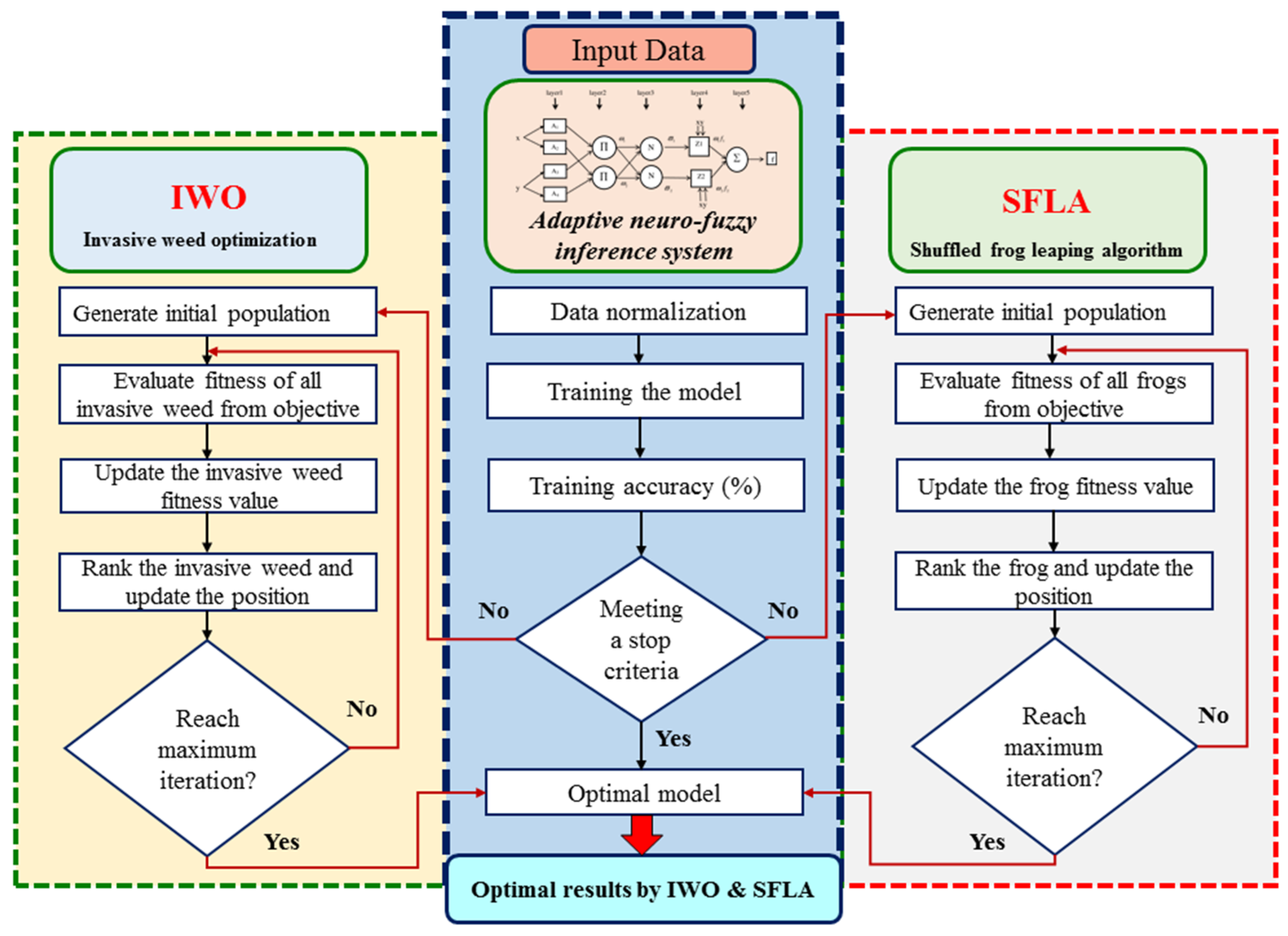
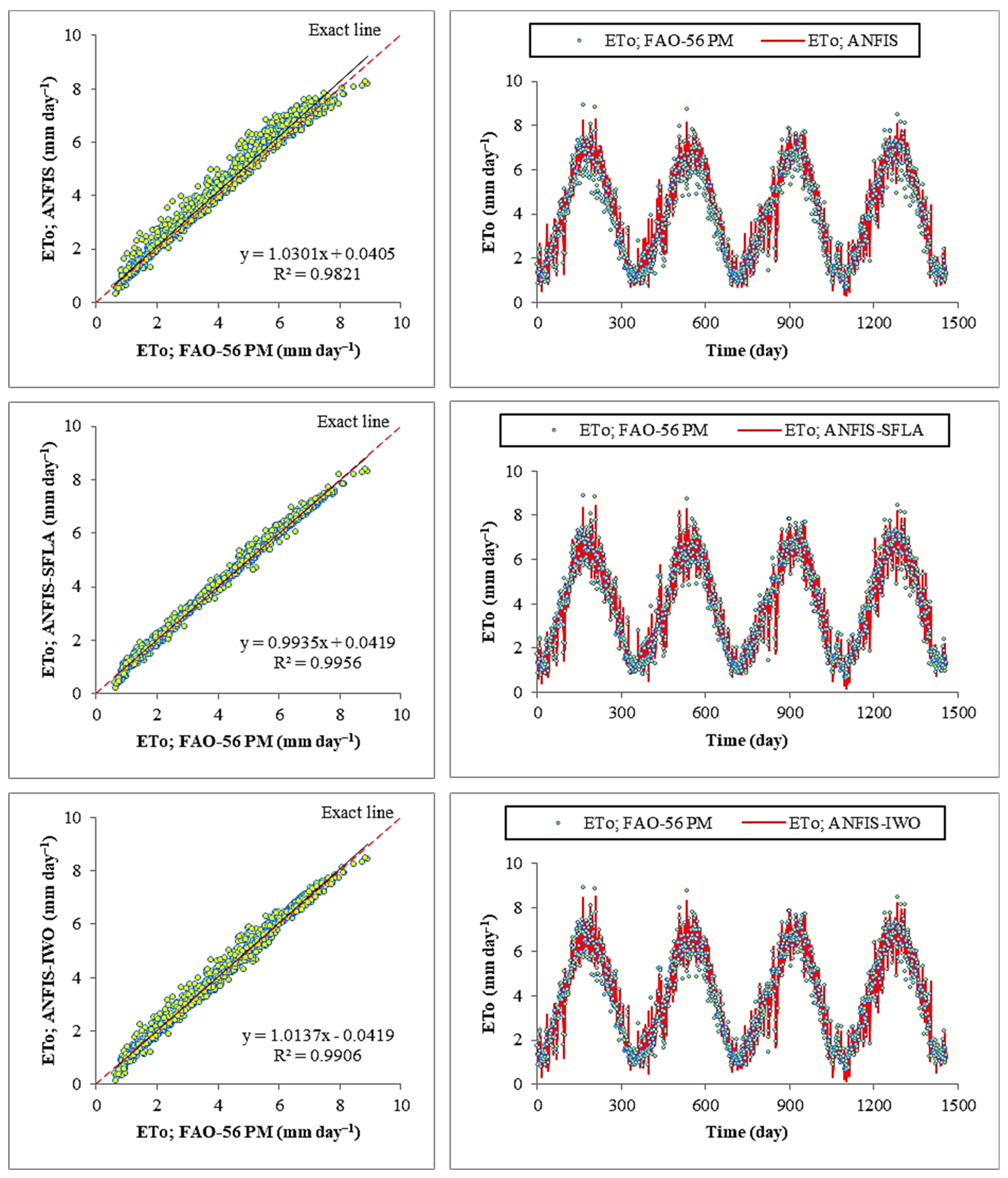
2.3. Adaptive Neuro-Fuzzy Inference System (ANFIS)

The ANFIS model was introduced by Jang in 1993 for first time [43]. This model is similar to a multilayered artificial neural network, except that it also uses fuzzy logic in addition to learning artificial neural network algorithms [44]. An ANFIS model consists of five layers: the data entry layer, fuzzy rules weight calculation layer, obtained weight normalization layer, rule calculation layer, summation layer, and network output layer. The distinguishing feature of ANFIS is the provision of a hybrid learning algorithm for the postdiffusion slope method and the least-squares method to modify the parameters [45]. In this research, the hybrid method was considered as the training model of the ANFIS model. Figure 3 shows a scheme of the ANFIS model used.

2.4. Shuffled Frog-Leaping Algorithm (SFLA)

The SFLA is a bio-inspired optimization algorithm that is based on the social behavior of frogs, and it belongs to the category of memetic algorithms [46]. The SAFLA is a metaheuristic optimization algorithm, and this metaheuristic algorithm is a swarm intelligence-based approach that is used for solving complexities of large optimization issues. The main idea behind this algorithm is to apply a local search method within the structure of the genetic algorithm to improve the aqueous work of the resonance process during the search. The metaheuristic algorithm first encodes the sum of the initial solutions, then it calculates the desirability of each answer based on a fitness function and generates new ones [47].

The function of this algorithm is to convert the original set into a number of smaller sets and then rearrange them with the competitive complex evolution (CCE) technique, and again by merging the ordered subsets of the original set that it makes one step more orderly and does it over and over to obtain the most optimal answers [48]. In the SFLA algorithm, the algorithm that performs this sorting on the subsets is called FLA, which is the CCE optimized and refined algorithm. In CCE, sorting into a complexity is done by subpopulations of the main population, but in FLA, this is done first on one memeplex and then on all memeplexes to always obtain the best answer out of all possible answers [46].

2.5. Invasive Weed Optimization (IWO)

The IWO is a type of sensible and evolutionary optimization algorithm that was first introduced by Mehrabian and Lucas [49], and was inspired via the procedure of proliferation, survival, and adaptability of weeds. Consistent with the IWO definition, a weed is a plant that produces and grows in unwanted places, and is a serious pest for other plants and forestalls their growth. This set of rules, whilst easy, is very effective and fast in finding the optimal factors and operates based on the basic and natural traits of weeds along with seed production, growth, and survival conflict in a colony.

First, a limited initial population is randomly generated and scattered in the problem-solving space. When determining the amount of initial population and reproduction, in IWO optimization method, every member of the population produces seeds according to its capabilities [50]. The product varies linearly from the smallest possible number of seeds to the largest number, and the weeds produce more seeds with better adaptation so that the mean is zero and the standard deviation varies at different stages, ensuring that the randomly distributed seeds are very close to their parent plant. In competitive Elimination, in the invasive weed algorithm, after several repetition steps, the number of clonal seeds reaches its maximum due to reproduction, and then a mechanism is used to remove weak seeds. Whilst the maximum number of seeds allowed is produced, every seed can produce new seeds, in keeping with the method noted in the previous steps, that can be scattered inside the space in question. When all the seeds are distributed within the location, every seed is given a rating, and inside the last level, the seeds with a lower rating are removed so that the seed population remains at the maximum. These steps are repeated until the seeds converge step by step to the optimal seed [49].

2.6. Hybrid Models (ANFIS-SFLA and ANFIS-IWO)

The main objective of the current study was application of the new hybrid models used for hydrological goals, the ANFIS-SFLA and ANFIS-IWO hybrid models, by comparison with the ordinary ANFIS to acquire an accurate and capable approach for simulating ETo at the study areas. The efficiency of the SFLA and IWO algorithms based on the ordinary ANFIS was defined by the optimized weight in the ANFIS by the shuffled frog-leaping and invasive weed optimization algorithms. When a mathematical function reaches a certain fitness between ANFIS weights and the SFAL and IWO, then hybrid models (i.e., ANFIS-SFLA and ANFIS-IWO) stop, or when iterations reach the maximum number, then model stops. This approach allows the models reach to their maximum capabilities, and then the new hybrid model can have advantages of both the ANFIS and optimization algorithms for estimation [48]. Previous studies have proven that such coupled optimized techniques can provide better results in hydrological modeling [50,51,52].

Table 3. Parameter settings for ANFIS, IWO, and SFLA.

ANFIS		IWO		SFLA
Epoch	1000	Maximum number of iterations	500	Maximum number of iterations	500
Initial step size	0.01	Number of initial population	25	Population size	40
Step size decrease	0.9	Maximum number of plant population	35	Number of memeplexes	5
Step size increase	1.1	Minimum number of seeds	1	Number of offspring	3
Error goal	0	Maximum number of seeds	15	Memeplex size	10

provides the optimal parameters related to the machine learning models used. Figure 4 demonstrates a schematic flowchart of the modeling process of current study.

2.7. Evaluation of the Model Performance

The present study proposed two novel hybrid models for modeling the daily ETo via the combination of ANFIS with SFLA and IWO. So, the hybrid ANFIS-SFLA and ANFIS-IWO models were developed. In addition, four empirical models, including Hargreaves–Samani, Romanenko, Priestly–Taylor, and Valiantzas, were utilized. The modeling accuracies of classic ANFIS, the hybrid ANFIS-SFLA, and ANFIS-IWO, as well as the original and calibrated forms of the empirical models, were compared with each other utilizing five evaluation metrics, including the root-mean-square error (RMSE), relative RMSE (RRMSE), mean absolute error (MAE), coefficient of determination (R²), and Nash–Sutcliffe efficiency (NSE). The mentioned metrics can be defined as follows:

$$RMSE=\sqrt{\frac{{{\displaystyle \sum }}_{i=1}^N{\left(E{T}_o^{i,F}-E{T}_o^{i,m}\right)}^2}{N}}$$

(1)

$$RRMSE=\frac{\sqrt{\frac{{{\displaystyle \sum }}_{i=1}^N{\left(E{T}_o^{i,F}-E{T}_o^{i,m}\right)}^2}{N}}}{\overline{E{T}_o^{i,F}}}\times 100\%$$

(2)

$$MAE=\frac{{{\displaystyle \sum }}_{i=1}^N\left|E{T}_o^{i,F}-E{T}_o^{i,m}\right|}{N}$$

(3)

$$R^2={\left. [\frac{{{\displaystyle \sum }}_{i=1}^N\left(E{T}_o^{i,F}-\overline{E{T}_o^{i,F}}\right)\cdot \left(E{T}_o^{i,m}-\overline{E{T}_o^{i,m}}\right)}{\sqrt{{{\displaystyle \sum }}_{i=1}^N{\left(E{T}_o^{i,F}-\overline{E{T}_o^{i,F}}\right)}^2\cdot {{\displaystyle \sum }}_{i=1}^N{\left(E{T}_o^{i,m}-\overline{E{T}_o^{i,m}}\right)}^2}}\right]}^2$$

(4)

$$NSE=1-\frac{{{\displaystyle \sum }}_{i=1}^N{\left(E{T}_o^{i,F}-E{T}_o^{i,m}\right)}^2}{{{\displaystyle \sum }}_{i=1}^N{\left(E{T}_o^{i,F}-\overline{E{T}_o^{i,F}}\right)}^2}$$

(5)

where $E{T}_o^{i,F}$, $E{T}_o^{i,m}$, $\overline{E{T}_o^{i,F}}$, $\overline{E{T}_o^{i,m}}$, and N represent the daily FAO-56 PM ETo; the modeled daily ETo through the classic ANFIS, the hybrid ANFIS-SFLA and ANFIS-IWO models, and the empirical models; the average of the daily FAO-56 PM ETo values; the average of the modeled daily ETo; and total number of observational values, respectively.

Among the aforementioned error statistics, the RRMSE and NSE can illustrate the accuracy of any modeling approach as below:

For the RRMSE:

Excellent (RRMSE < 10%); good (10% < RRMSE < 20%); fair (20% < RRMSE < 30%), and poor (RRMSE > 30%) [53].

For the NSE:

Very good ($0.75<NSE\le 1.0$); good ($0.65<NSE\le 0.75$); satisfactory ($0.50<NSE\le 0.65$); acceptable ($0.40<NSE\le 0.50$), and unsatisfactory ($NSE\le 0.40$) [54].

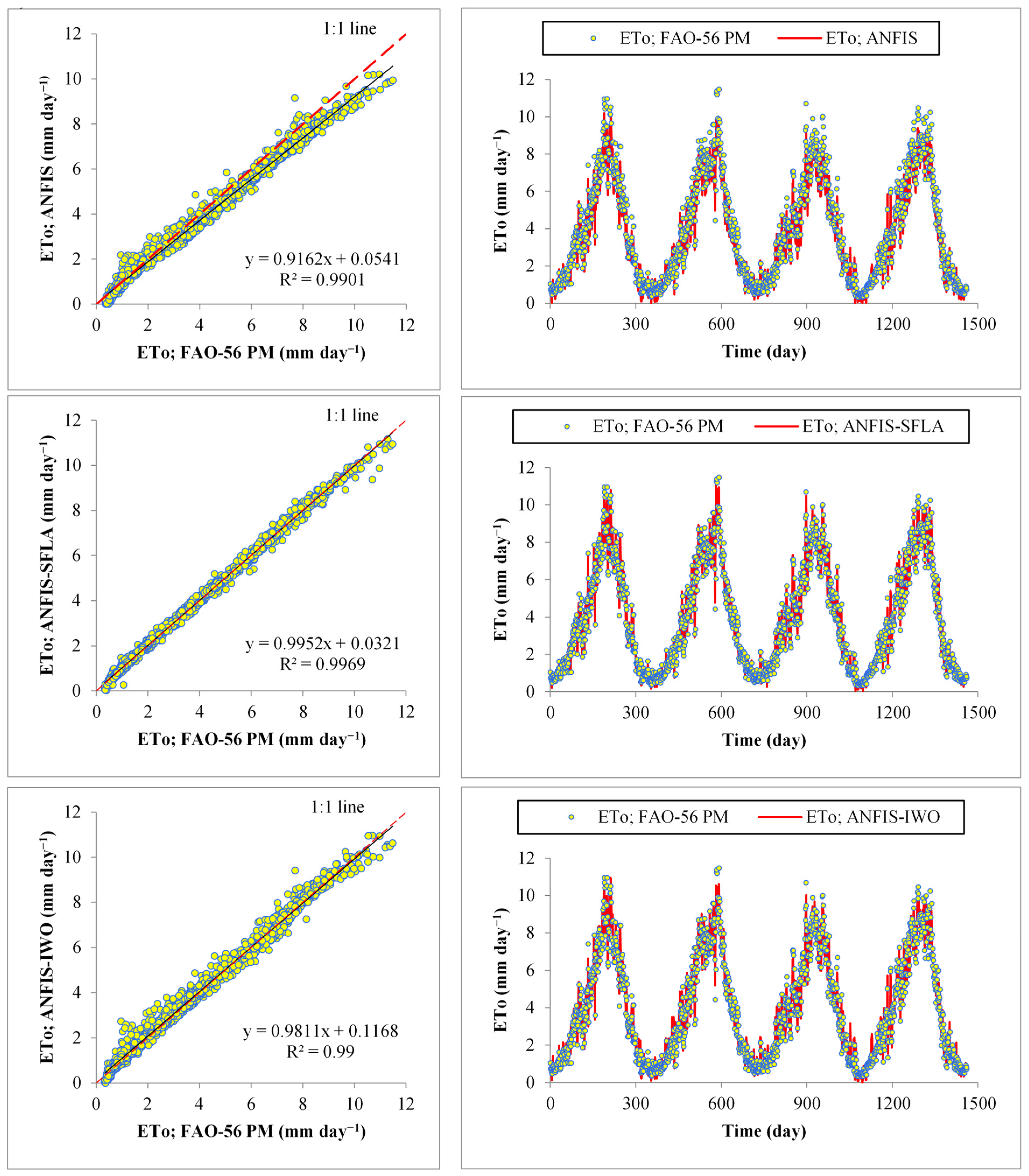
3. Results and Discussion

Firstly, the classic ANFIS was implemented at the study sites based on the input combinations defined in

Table 4. Inputs applied for developing the classical ANFIS and the two hybrid models (ANFIS-SFLA and ANFIS-IWO). Symbols are explained in Section 2.1 and in the footnote of Table 2.

Model No.	Inputs	Output
M1	Tmin, Tmax, T	ETo
M2	Tmin, Tmax, T, SSD	ETo
M3	Tmin, Tmax, T, SSD, U2	ETo
M4	Tmin, Tmax, T, SSD, U2, RH	ETo
M5	Tmin, Tmax, T, SSD, U2, RH, es-ea	ETo
M6	Tmin, Tmax, T, SSD, U2, RH, es-ea, Rs	ETo
M7	Tmin, Tmax, T, SSD, U2, RH, es-ea, Rs, Rn, Ra	ETo

. As seen in the table, seven various scenarios (i.e., M1–M7) were taken into consideration in the modeling procedure. The RMSE, RRMSE, MAE, R², and NSE statistical parameters obtained by the classic ANFIS at Tabriz and Shiraz stations are respectively presented in the first sections of

Table 5. The statistical indicators obtained for the classical ANFIS and the proposed hybrid ANFIS-SFLA and ANFIS-IWO models in estimating daily ETo vs. the standard daily ETo calculated with the FAO-56 PM method in the training and test phases (Tabriz station).

Models	Model No.	Training					Test
		RMSE (mm day−1)	RRMSE (%)	MAE (mm day−1)	R2	NSE	RMSE (mm day−1)	RRMSE (%)	MAE (mm day−1)	R2	NSE
ANFIS	M1	0.90	23.22	0.71	0.88	0.88	0.93	23.63	0.72	0.90	0.88
	M2	0.81	21.07	0.64	0.90	0.90	0.86	21.85	0.67	0.92	0.90
	M3	0.59	15.25	0.48	0.95	0.95	0.60	15.10	0.48	0.95	0.95
	M4	0.57	14.83	0.47	0.95	0.95	0.58	14.73	0.48	0.96	0.95
	M5	0.58	15.01	0.49	0.96	0.95	0.55	14.06	0.46	0.97	0.96
	M6	0.51	13.14	0.42	0.97	0.96	0.40	10.27	0.31	0.98	0.97
	M7	0.42	10.87	0.33	0.98	0.97	0.44	11.26	0.35	0.99	0.97
ANFIS-SFLA	M1	0.86	22.28	0.68	0.89	0.89	0.86	21.81	0.67	0.91	0.90
	M2	0.75	19.42	0.58	0.91	0.91	0.77	19.47	0.59	0.93	0.92
	M3	0.46	11.91	0.37	0.96	0.96	0.46	11.62	0.36	0.97	0.97
	M4	0.39	10.14	0.30	0.97	0.97	0.39	9.99	0.30	0.98	0.98
	M5	0.40	10.38	0.32	0.97	0.97	0.37	9.46	0.30	0.98	0.98
	M6	0.32	8.33	0.25	0.98	0.98	0.33	8.54	0.26	0.98	0.98
	M7	0.14	3.78	0.10	0.99	0.99	0.15	3.96	0.11	0.99	0.99
ANFIS-IWO	M1	0.85	21.94	0.66	0.89	0.89	0.84	21.26	0.65	0.91	0.90
	M2	0.77	19.88	0.60	0.91	0.91	0.81	20.42	0.63	0.92	0.91
	M3	0.52	13.44	0.42	0.96	0.96	0.56	14.12	0.44	0.96	0.96
	M4	0.48	12.40	0.40	0.96	0.96	0.47	12.05	0.40	0.97	0.97
	M5	0.50	13.00	0.40	0.96	0.96	0.48	12.31	0.39	0.97	0.97
	M6	0.38	10.00	0.30	0.97	0.97	0.39	9.80	0.29	0.98	0.98
	M7	0.28	7.26	0.19	0.98	0.98	0.28	7.18	0.19	0.99	0.99

Note: bold values denote the error criteria for the best-performing model in the training and test phases.

and

Table 6. The statistical indicators obtained for the classical ANFIS and the proposed hybrid ANFIS-SFLA and ANFIS-IWO models in estimating daily ETo vs. the standard daily ETo calculated with the FAO-56 PM method in the training and test phases (Shiraz station).

Models	Model No.	Training					Test
		RMSE (mm day−1)	RRMSE (%)	MAE (mm day−1)	R2	NSE	RMSE (mm day−1)	RRMSE (%)	MAE (mm day−1)	R2	NSE
ANFIS	M1	0.93	22.73	0.75	0.81	0.80	0.87	22.02	0.70	0.83	0.81
	M2	0.81	19.89	0.65	0.86	0.85	0.74	18.74	0.59	0.87	0.86
	M3	0.52	12.62	0.41	0.94	0.94	0.48	12.22	0.40	0.94	0.94
	M4	0.53	13.02	0.43	0.95	0.93	0.52	13.31	0.42	0.94	0.93
	M5	0.54	13.30	0.43	0.95	0.93	0.51	12.94	0.42	0.94	0.93
	M6	0.52	12.72	0.40	0.96	0.94	0.47	12.00	0.37	0.96	0.94
	M7	0.32	7.98	0.22	0.98	0.97	0.33	8.34	0.22	0.98	0.97
ANFIS-SFLA	M1	0.89	21.68	0.71	0.82	0.82	0.82	20.79	0.66	0.83	0.83
	M2	0.71	17.39	0.55	0.88	0.88	0.65	16.59	0.51	0.89	0.89
	M3	0.39	9.51	0.30	0.96	0.96	0.40	10.10	0.30	0.96	0.96
	M4	0.35	8.69	0.28	0.97	0.97	0.35	8.88	0.27	0.97	0.97
	M5	0.35	8.63	0.28	0.97	0.97	0.35	9.06	0.29	0.96	0.96
	M6	0.30	7.28	0.23	0.98	0.98	0.25	6.42	0.20	0.98	0.98
	M7	0.13	3.33	0.09	0.99	0.99	0.13	3.41	0.09	0.99	0.99
ANFIS-IWO	M1	0.89	21.71	0.71	0.82	0.82	0.83	21.13	0.66	0.83	0.83
	M2	0.75	18.28	0.59	0.87	0.87	0.69	17.53	0.55	0.88	0.88
	M3	0.41	10.17	0.32	0.96	0.96	0.41	10.40	0.32	0.96	0.95
	M4	0.44	10.81	0.35	0.95	0.95	0.42	10.73	0.34	0.95	0.95
	M5	0.41	10.10	0.33	0.96	0.96	0.41	10.41	0.33	0.95	0.95
	M6	0.40	9.75	0.31	0.96	0.96	0.36	9.24	0.29	0.96	0.96
	M7	0.20	4.95	0.14	0.99	0.99	0.20	5.13	0.15	0.99	0.99

Note: bold values denote the error criteria for the best-performing model at the training and test phases.

for both training and test periods. It can obviously be seen that the M1-based ANFIS model with minimal inputs (i.e., temperature components) presented the worst performance at both of the study stations. Generally, the accuracy of classic ANFIS was enhanced by increasing the number of input predictors; however, there was a negligible difference between the performances of the M1 and M2 models at the studied regions. On the other hand, the inclusion of the wind speed (U2) in the M2 model (i.e., M3 model) led to further improvement of the performance of the classic ANFIS. This outcome confirmed the results of previous works [55,56] in that, although wind speed solely showed the lowest accuracy in ETo modeling, considering this parameter along with the other meteorological parameters improved the ETo modeling performance. In addition, slight discrepancies were observed when comparing the accuracy of the M3–M6 models of the classic ANFIS. The M7 models developed at the study locations outperformed the M1–M6 models. This model utilized full inputs for modeling the ETo. The difference between the M6 and M7 models was that two radiation components (i.e., Rn and Ra) were considered in the M7 model. The Ra was calculated by means of the Julian day and latitude of the location. Moreover, minimum temperature, maximum temperature, and sunshine duration ratio were required to compute the Rn. The required parameters for calculating the Ra and Rn were generally available at all locations. Therefore, we concluded that considering them could be of use in enhancing the accuracy of modeling techniques in estimating the ETo.

Novel hybrid models were then developed and proposed to improve the performance of the classic ANFIS. For this, two optimization algorithms, including the SFLA and IWO, were coupled on the classic ANFIS. The statistical results of the novel hybrid models at Tabriz and Shiraz stations are shown in the second and third sections of Table 5 and Table 6, respectively. The results obtained for the classic ANFIS were also observed in the hybrid ANFIS-SFLA and ANFIS-IWO models. The same results were obtained: the worst performance by M1 models; enhanced performance of hybrid models by increasing the number of variables/predictors as inputs; and the superiority of the M7 models compared with the M1–M6 models. As was apparent, hybridizing the ANFIS with SFLA and IWO algorithms remarkably improved the forecasting efficacy of classic ANFIS. For an instance, the error statistics of the RMSE, RRMSE, MAE, R², and NSE for the M7-based classic ANFIS during the test phase were obtained respectively as 0.44 mm day⁻¹, 11.26%, 0.35 mm day⁻¹, 0.99, and 0.97 at Tabriz station; and 0.33 mm day⁻¹, 8.34%, 0.22 mm day⁻¹, 0.98, and 0.97 at Shiraz station; while the aforementioned error criteria were improved by the ANFIS-SFLA (i.e., 0.15 mm day⁻¹, 3.96%, 0.11 mm day⁻¹, 0.99, and 0.99 at Tabriz station; 0.13 mm day⁻¹, 3.41%, 0.09 mm day⁻¹, 0.99, and 0.99 at Shiraz station) and ANFIS-IWO (i.e., 0.28 mm day⁻¹, 7.18%, 0.19 mm day⁻¹, 0.99, and 0.99 at Tabriz station; 0.20 mm day⁻¹, 5.13%, 0.15 mm day⁻¹, 0.99, and 0.99 at Shiraz station). The results confirmed the outcomes of previous works [27,28,29,30,37,57,58] in that coupling the optimization algorithms and ML techniques could improve modeling of the ETo time series in comparison with the standalone ML techniques.

Figure 5 and Figure 6 show a comparison of the superior hybrid models (i.e., M7 models of ANFIS-SFLA and ANFIS-IWO) and the corresponding M7 model of the classic ANFIS at Tabriz and Shiraz stations, respectively. Lesser dispersions of the data points around the exact line (i.e., 1:1) in the proposed hybrid models, particularly for the ANFIS-SFLA, confirmed the higher accuracy of the coupled models over the single ANFIS. On the other hand, the time series plots of the hybrid models denoted the reliable capability of the proposed models for capturing the daily FAO-56 PM ETo values in comparison with the classic ANFIS. This point is very clear about the modeling of peak points, in that the modeled values of daily ETo via the hybrid models were much closer to the daily FAO-56 PM ETo data. In this regard, the classic ANFIS presented poor performances. Furthermore, hydrograph plots clearly showed the efficiencies of the classic ANFIS. The hybrid ANFIS-SFLA and ANFIS-IWO performed better in modeling the low and medium values than the peak points.

In addition to the application of ANFIS and proposing the novel hybrid models, four types of empirical models (Table 2) were used in this study. The values of error criteria obtained by the original versions of the equations at the Tabriz and Shiraz stations are tabulated in

Table 7. The statistical indicators computed for the original and calibrated empirical equations in the training and test phases (Tabriz station).

Equations	Train					Test
	RMSE (mm day−1)	RRMSE (%)	MAE (mm day−1)	R2	NSE	RMSE (mm day−1)	RRMSE (%)	MAE (mm day−1)	R2	NSE
Original Hargreaves–Samani	1.11	28.72	0.74	0.91	0.82	1.23	31.07	0.79	0.90	0.80
Original Romanenko	2.32	59.91	1.63	0.86	0.22	2.03	51.12	1.37	0.89	0.47
Original Priestly–Taylor	1.49	38.60	1.10	0.89	0.67	1.62	40.82	1.15	0.89	0.66
Original Valiantzas	0.57	14.74	0.41	0.96	0.95	0.74	18.81	0.61	0.98	0.92
Calibrated Hargreaves–Samani	0.79	20.38	0.57	0.91	0.91	0.85	21.42	0.60	0.90	0.90
Calibrated Romanenko	1.01	26.14	0.76	0.86	0.85	1.03	25.98	0.77	0.89	0.86
Calibrated Priestly–Taylor	0.88	22.84	0.63	0.89	0.88	0.92	23.29	0.62	0.89	0.89
Calibrated Valiantzas	0.47	12.16	0.36	0.96	0.96	0.46	11.76	0.37	0.98	0.97

Note: bold values denote the error criteria for the best-performing empirical model in the training and test phases.

and

Table 8. The statistical indicators computed for the original and calibrated empirical equations in the training and test phases (Shiraz station).

Equations	Train					Test
	RMSE (mm day−1)	RRMSE (%)	MAE (mm day−1)	R2	NSE	RMSE (mm day−1)	RRMSE (%)	MAE (mm day−1)	R2	NSE
Original Hargreaves–Samani	0.94	22.85	0.75	0.86	0.80	1.00	25.48	0.80	0.88	0.75
Original Romanenko	4.30	104.51	3.56	0.82	−3.06	4.41	111.65	3.57	0.83	−3.73
Original Priestly–Taylor	1.00	24.34	0.73	0.90	0.77	0.89	22.49	0.65	0.91	0.80
Original Valiantzas	0.96	23.48	0.84	0.94	0.79	0.90	22.74	0.79	0.97	0.80
Calibrated Hargreaves–Samani	0.78	19.10	0.60	0.86	0.86	0.75	19.09	0.58	0.88	0.86
Calibrated Romanenko	0.94	23.00	0.74	0.82	0.80	0.90	22.75	0.71	0.83	0.80
Calibrated Priestly–Taylor	0.66	16.14	0.50	0.90	0.90	0.58	14.86	0.45	0.91	0.91
Calibrated Valiantzas	0.44	10.74	0.31	0.95	0.95	0.27	7.06	0.22	0.98	0.98

Note: bold values denote the error criteria for the best-performing empirical model at the training and test phases.

, respectively. The Romanenko equation yielded the weakest performance among the empirical equations, especially at Shiraz station. Additionally, the Valiantzas equation was the best-performing empirical model at the study sites. It was obvious that the empirical models should be calibrated in the study areas to provide the best performance.

Table 9. The calibrated forms of empirical models applied in this study.

Stations	Empirical Models	Equations
Tabriz	Hargreaves–Samani	$E{T}_o=\frac{1}{\lambda }0.0028R_a\left(T+17.8\right){\left(T_{max}-T_{min}\right)}^{0.5}$
	Romanenko	$E{T}_o=0.00004{(T+25)}^2\left(100-RH\right)$
	Priestly–Taylor	$E{T}_o=1.7077\frac{\Delta }{\Delta +\gamma }\frac{R_n-G}{\lambda }$
	Valiantzas	$E{T}_o=0.025252R_s\sqrt{\left|T+9.5\right|}-0.07853R_s^{0.6}{\phi }^{0.15}+0.06109\left(T+20\right)\left(1-\frac{RH}{100}\right)U_2^{0.7}$
Shiraz	Hargreaves–Samani	$E{T}_o=\frac{1}{\lambda }0.0021R_a\left(T+17.8\right){\left(T_{max}-T_{min}\right)}^{0.5}$
	Romanenko	$E{T}_o=0.00003{(T+25)}^2\left(100-RH\right)$
	Priestly–Taylor	$E{T}_o=1.5062\frac{\Delta }{\Delta +\gamma }\frac{R_n-G}{\lambda }$
	Valiantzas	$E{T}_o=0.02451R_s\sqrt{\left|T+9.5\right|}-0.102R_s^{0.6}{\phi }^{0.15}+0.060782\left(T+20\right)\left(1-\frac{RH}{100}\right)U_2^{0.7}$

reports the calibrated versions of the empirical models used. According to the statistical indicators obtained for the calibrated empirical models in Table 7 and Table 8, it can be observed that the calibration procedure significantly improved the performance of empirical models over their original versions. The better-performing models were the calibrated forms of the Valiantzas (followed by Hargreaves–Samani) at Tabriz station, and the Valiantzas and Priestley–Taylor equations at Shiraz station. The calibrated Valiantzas equation performed the best for both studied sites in all statistical indicators (RMSE = 0.46 mm day⁻¹, RRMSE = 11.76%, MAE = 0.37 mm day⁻¹, R² = 0.98, NSE = 0.97 in the test stage for Tabriz station; RMSE = 0.27 mm day⁻¹, RRMSE = 7.06%, MAE = 0.22 mm day⁻¹, R² = 0.98, NSE = 0.98 in the test stage for Shiraz station).

Figure 7 and Figure 8 show the comparative graphs of the daily ETo estimates from the FAO-56 PM method against the modeled data by the best empirical model (i.e., calibrated Valiantzas) and its original form. Fewer dispersions were visible around the exact line (1:1) in the calibrated Valiantzas model compared with the original Valiantzas. Moreover, overestimation (i.e., red lines in the hydrograph plots) can be seen in many of data points in the original Valiantzas at the study locations, especially at Shiraz station; however, this overestimation was corrected by the calibrated version of this model.

Here, the modeling performances of the classic ANFIS, hybrid ANFIS-SFLA and ANFIS-IWO models, and empirical models in the original and calibrated forms were compared with each other. It is obvious from Table 4 and Table 5 that the hybrid ANFIS-SFLA and ANFIS-IWO models developed at the study sites presented superior results compared with the classic ANFIS; however, the ANFIS-SFLA outperformed the ANFIS-IWO. Moreover, as mentioned previously, the calibrated empirical models yielded better estimates of the daily ETo than the original forms of empirical models. A performance assessment of the classic and proposed coupled models with the empirical models in their original and calibrated forms revealed that the original empirical models generally provided the weakest performances. Among the empirical models applied, the calibrated Valiantzas model illustrated better accuracy than the M1–M6 models of classic ANFIS at both stations, M1 and M2 models of ANFIS-SFLA, M1–M5 models of ANFIS-IWO at both phases of the Tabriz station; M1–M2 (training phase) and M1–M5 (test phase) models of ANFIS-SFLA; as well as M1, M2, and M4 models of ANFIS-IWO at the training stage and M1–M6 models of ANFIS-IWO at the test stage of Shiraz station. We concluded that the calibrated version of the Valiantzas model could be of use in modeling the daily ETo with a high degree of precision; therefore, this model could be compatible with the hybrid models proposed in the present study. In general, the M7 models of ANFIS, ANFIS-SFLA, and ANFIS-IWO performed much better than the calibrated empirical models; however, the M7 models of ANFIS-SFLA developed at the Tabriz and Shiraz stations were the best-performing techniques for modeling of the daily ETo with a dependable accuracy.

In this section, the modeling accuracy of all applied models is qualitatively described based on the various ranges for the RRMSE and NSE criteria. In terms of the NSE statistic, the accuracy of the classic ANFIS, the hybrid ANFIS-SFLA and ANFIS-IWO, and the calibrated forms of empirical models was located in the “very good” class, since the values of NSE for the mentioned models were in the range of 0.75–1.0. Similarly, the performance of the original Hargreaves–Samani and Valiantzas at Tabriz and Shiraz stations, as well as the Priestly–Taylor equation at Shiraz station, belonged to the “very good” category. The accuracy class of the original Priestly–Taylor model at Tabriz station was “good”, since 0.65 < NSE ≤ 0.75. Finally, the original Romanenko belonged to the “unsatisfactory” class at both locations. The performance of applied models was then classified based on the RRMSE criterion. The M1 and M2 models of the classic ANFIS at Tabriz station, the M1 model of the classic ANFIS at Shiraz station, as well as the M1 models of ANFIS-SFLA and ANFIS-IWO at both of the stations were located in the “fair” degree (20% < RRMSE < 30%). In addition, at Tabriz station, the performance of the M6 and M7 models of ANFIS-SFLA during the training stage, M4–M7 models of ANFIS-SFLA during the test stage, the M7 model of ANFIS-IWO in training, and the M6–M7 models of ANFIS-IWO in the test period were classified in the “excellent” class. For the case of Shiraz station, the M7 models of classic ANFIS, M3–M7 models of ANFIS-SFLA (training stage) and M4–M7 models of this technique, as well as the M6–M7 models of ANFIS-IWO, were found to belong to the “excellent” class. Regarding the classes of empirical models, it can be clearly seen in Table 6 and Table 7 that the accuracy class of the original Romanenko model was poor, especially at Shiraz station. As is clear, the performance class of excellent was not observed for the empirical models in their original and calibrated forms, with the exception of the calibrated Valiantzas in the test stage at Shiraz station. The best class of empirical models was obtained by the original and calibrated versions of the Valiantzas model at Tabriz and Shiraz stations, and the calibrated Priestly–Taylor model at Shiraz station.

Given that the ETo equations were developed in specific areas and with the climatic conditions of that location, it is therefore necessary to calibrate these equations with reliable reference data before use in other areas. In other words, none of the empirical equations met the needs of all climatic conditions, and only met the specific conditions in which they were developed. Besides, evapotranspiration as a climatic variable is affected by their regional and climatic characteristics. For this, calibration of empirical models is a basic requirement to achieve their better performance. The better accuracy of calibrated equations over their original ones justify this issue.

Moreover, the same procedure should be taken into consideration when assessing the entire performance of the models used. In this context, the empirical models should be calibrated through the application of a training dataset, as used for the machine learning models. Finally, the performance of each empirical model can be evaluated by different types of supervised learning algorithms via machine learning models. Machine learning models, by finding and learning from patterns in a dataset, can understand the relationship between ETo and other meteorological variables, and they can be used as strong tools for prediction. Especially in the case of the limited availability of data, machine learning models can provide a satisfactory simulation, even with a minimum dataset. In addition, optimization algorithms can be used as boosting tool for improving the ability of the ordinary ANFIS model for ETo prediction. We recommend that other potential researchers apply different types of newly developed machine learning models to evaluate and reach the highest accuracy in ETo prediction.

4. Conclusions

An attempt was made in the present study to improve the modeling accuracy of the ANFIS in daily ETo estimation. The Tabriz and Shiraz stations in Iran were selected as the two studied sites. The classic ANFIS was coupled with optimization algorithms such as SFLA and IWO. So, novel hybrid ANFIS-SFLA and ANFIS-IWO models were proposed and implemented. The classic and hybrid models were developed under seven models (M1–M7) utilizing different numbers of climatic variables as inputs. Evaluation results showed that the developed novel models demonstrated superiority over the classic ANFIS; however, the hybrid model ANFIS-SFLA provided better performances than ANFIS-IWO. Generally, the performances of the classic and coupled models were improved with an increasing number of predictors/variables. The M1 models with minimal inputs and M7 models with full predictors were the worst and best models in modeling the daily ETo, respectively. The M7 models of the hybrid ANFIS-SFLA were the best-performing models for precise modeling of the daily ETo time series at the studied sites. Four empirical models were also applied in this study, and then the performances of the empirical models were assessed in their original and calibrated forms. It was found that calibrating the empirical equations could improve the accuracy of the estimated daily ETo over their original forms. Among the empirical models, the Romanenko model showed the weakest results in its both original and calibrated versions. In contrast, the Valiantzas was the best model. A performance assessment of the classic ANFIS, hybrid ANFIS-SFLA, and ANFIS-IWO, as well as the original and calibrated empirical models, demonstrated that the implemented hybrid models, followed by the classic ANFIS (M3–M7 models), generally outperformed the empirical models. In addition, different empirical-based methods had different complexities, and some of them required more input data, which might be difficult to achieve. Therefore, there is a need to develop/improve methods with varying inputs to adapt to the real situation considering the availability of the data. This study hybridized an ML-based model (i.e., ANFIS) with the optimization algorithms, including the SFLA and IWO. Future research works could implement a variety of hybrid models for ETo modeling through coupling the ANFIS and SVM with the other types of bio-inspired optimizers, including the firefly algorithm (FA), whale optimization algorithm (WOA), krill herd algorithm (KHA), dragonfly algorithm (DFA), grasshopper optimization algorithm (GOA), etc. Similar to the case studies considered in the current work, the climate of a large part of Iran is arid or semiarid. Therefore, the estimation performance of implemented models in capturing the ETo time series can be evaluated in climates similar to that of Iran (and other parts of the world), and the obtained results could be compared with our findings in this study.

References

1. Gocić, M.; Motamedi, S.; Shamshirband, S.; Petković, D.; Ch, S.; Hashim, R.; Arif, M. Soft computing approaches for forecasting reference evapotranspiration. Comput. Electron. Agric. 2015, 113, 164–173. [Google Scholar] [CrossRef]
2. Yassin, M.A.; Alazba, A.A.; Mattar, M.A. Artificial neural networks versus gene expression programming for estimating reference evapotranspiration in arid climate. Agric. Water Manag. 2016, 163, 110–124. [Google Scholar] [CrossRef]
3. Kisi, O. Modeling reference evapotranspiration using three different heuristic regression approaches. Agric. Water Manag. 2016, 169, 162–172. [Google Scholar] [CrossRef]
4. Mehdizadeh, S.; Saadatnejadgharahassanlou, H.; Behmanesh, J. Calibration of Hargreaves–Samani and Priestley–Taylor equations in estimating reference evapotranspiration in the Northwest of Iran. Arch. Agron. Soil Sci. 2017, 63, 942–955. [Google Scholar] [CrossRef]
5. Feng, Y.; Peng, Y.; Cui, N.; Gong, D.; Zhang, K. Modeling reference evapotranspiration using extreme learning machine and generalized regression neural network only with temperature data. Comput. Electron. Agric. 2017, 136, 71–78. [Google Scholar] [CrossRef]
6. Mohammadi, B.; Mehdizadeh, S. Modeling daily reference evapotranspiration via a novel approach based on support vector regression coupled with whale optimization algorithm. Agric. Water Manag. 2020, 237, 106145. [Google Scholar] [CrossRef]
7. Zhang, B.; Liu, Y.; Xu, D.; Zhao, N.; Lei, B.; Rosa, R.D.; Paredes, P.; Paço, T.A.; Pereira, L.S. The dual crop coefficient approach to estimate and partitioning evapotranspiration of the winter wheat-summer maize crop sequence in North China Plain. Irrig. Sci. 2013, 31, 1303–1316. [Google Scholar] [CrossRef]
8. Kool, D.; Agam, N.; Lazarovitch, N.; Heitman, J.L.; Sauer, T.J.; Ben-Gal, A. A review of approaches for evapotranspiration partitioning. Agric. For. Meteorol. 2014, 184, 56–70. [Google Scholar] [CrossRef]
9. Bottazzi, M.; Bancheri, M.; Mobilia, M.; Bertoldi, G.; Longobardi, A.; Rigon, R. Comparing evapotranspiration estimates from the geoframe-prospero model with penman–monteith and priestley-taylor approaches under different climate conditions. Water 2021, 13, 1221. [Google Scholar] [CrossRef]
10. Allen, R.G.; Pereira, L.S.; Raes, D.; Smith, M. Crop Evapotranspiration—Guidelines for Computing Crop Water Requirements—FAO Irrigation and Drainage Paper 56; FAO: Rome, Italy, 1998; ISBN 9251042195. [Google Scholar]
11. Kumar, M.; Raghuwanshi, N.S.; Singh, R. Artificial neural networks approach in evapotranspiration modeling: A review. Irrig. Sci. 2011, 29, 11–25. [Google Scholar] [CrossRef]
12. Mosre, J.; Suárez, F. Actual evapotranspiration estimates in arid cold regions using machine learning algorithms with in situ and remote sensing data. Water 2021, 13, 870. [Google Scholar] [CrossRef]
13. Ahmadi, F.; Mehdizadeh, S.; Mohammadi, B.; Pham, Q.B.; Doan, T.N.C.; Vo, N.D. Application of an artificial intelligence technique enhanced with intelligent water drops for monthly reference evapotranspiration estimation. Agric. Water Manag. 2021, 244, 106622. [Google Scholar] [CrossRef]
14. Mohammadi, B.; Moazenzadeh, R.; Christian, K.; Duan, Z. Improving streamflow simulation by combining hydrological process-driven and artificial intelligence-based models. Environ. Sci. Pollut. Res. 2021, 28, 65752–65768. [Google Scholar] [CrossRef]
15. Elbeltagi, A.; Kumari, N.; Dharpure, J.K.; Mokhtar, A.; Alsafadi, K.; Kumar, M.; Mehdinejadiani, B.; Ramezani Etedali, H.; Brouziyne, Y.; Towfiqul Islam, A.R.M.; et al. Prediction of combined terrestrial evapotranspiration index (Ctei) over large river basin based on machine learning approaches. Water 2021, 13, 547. [Google Scholar] [CrossRef]
16. Torres, A.F.; Walker, W.R.; McKee, M. Forecasting daily potential evapotranspiration using machine learning and limited climatic data. Agric. Water Manag. 2011, 98, 553–562. [Google Scholar] [CrossRef]
17. Ladlani, I.; Houichi, L.; Djemili, L.; Heddam, S.; Belouz, K. Modeling daily reference evapotranspiration (ET 0) in the north of Algeria using generalized regression neural networks (GRNN) and radial basis function neural networks (RBFNN): A comparative study. Meteorol. Atmos. Phys. 2012, 118, 163–178. [Google Scholar] [CrossRef]
18. Kisi, O.; Cengiz, T.M. Fuzzy Genetic Approach for Estimating Reference Evapotranspiration of Turkey: Mediterranean Region. Water Resour. Manag. 2013, 27, 3541–3553. [Google Scholar] [CrossRef]
19. Abdullah, S.S.; Malek, M.A.; Abdullah, N.S.; Kisi, O.; Yap, K.S. Extreme Learning Machines: A new approach for prediction of reference evapotranspiration. J. Hydrol. 2015, 527, 184–195. [Google Scholar] [CrossRef]
20. Wen, X.; Si, J.; He, Z.; Wu, J.; Shao, H.; Yu, H. Support-Vector-Machine-Based Models for Modeling Daily Reference Evapotranspiration With Limited Climatic Data in Extreme Arid Regions. Water Resour. Manag. 2015, 29, 3195–3209. [Google Scholar] [CrossRef]
21. Wang, S.; Fu, Z.Y.; Chen, H.S.; Nie, Y.P.; Wang, K.L. Modeling daily reference ET in the karst area of northwest Guangxi (China) using gene expression programming (GEP) and artificial neural network (ANN). Theor. Appl. Climatol. 2016, 126, 493–504. [Google Scholar] [CrossRef]
22. Traore, S.; Luo, Y.; Fipps, G. Deployment of artificial neural network for short-term forecasting of evapotranspiration using public weather forecast restricted messages. Agric. Water Manag. 2016, 163, 363–379. [Google Scholar] [CrossRef]
23. Mehdizadeh, S. Estimation of daily reference evapotranspiration (ETo) using artificial intelligence methods: Offering a new approach for lagged ETo data-based modeling. J. Hydrol. 2018, 559, 794–812. [Google Scholar] [CrossRef]
24. Mattar, M.A. Using gene expression programming in monthly reference evapotranspiration modeling: A case study in Egypt. Agric. Water Manag. 2018, 198, 23–38. [Google Scholar] [CrossRef]
25. Sanikhani, H.; Kisi, O.; Maroufpoor, E.; Yaseen, Z.M. Temperature-based modeling of reference evapotranspiration using several artificial intelligence models: Application of different modeling scenarios. Theor. Appl. Climatol. 2019, 135, 449–462. [Google Scholar] [CrossRef]
26. Saggi, M.K.; Jain, S. Reference evapotranspiration estimation and modeling of the Punjab Northern India using deep learning. Comput. Electron. Agric. 2019, 156, 387–398. [Google Scholar] [CrossRef]
27. Ozkan, C.; Kisi, O.; Akay, B. Neural networks with artificial bee colony algorithm for modeling daily reference evapotranspiration. Irrig. Sci. 2011, 29, 431–441. [Google Scholar] [CrossRef]
28. Eslamian, S.S.; Gohari, S.A.; Zareian, M.J.; Firoozfar, A. Estimating Penman-Monteith Reference Evapotranspiration Using Artificial Neural Networks and Genetic Algorithm: A Case Study. Arab. J. Sci. Eng. 2012, 37, 935–944. [Google Scholar] [CrossRef]
29. Yin, Z.; Wen, X.; Feng, Q.; He, Z.; Zou, S.; Yang, L. Integrating genetic algorithm and support vector machine for modeling daily reference evapotranspiration in a semi-arid mountain area. Hydrol. Res. 2017, 48, 1177–1191. [Google Scholar] [CrossRef]
30. Tao, H.; Diop, L.; Bodian, A.; Djaman, K.; Ndiaye, P.M.; Yaseen, Z.M. Reference evapotranspiration prediction using hybridized fuzzy model with firefly algorithm: Regional case study in Burkina Faso. Agric. Water Manag. 2018, 208, 140–151. [Google Scholar] [CrossRef]
31. Wu, L.; Zhou, H.; Ma, X.; Fan, J.; Zhang, F. Daily reference evapotranspiration prediction based on hybridized extreme learning machine model with bio-inspired optimization algorithms: Application in contrasting climates of China. J. Hydrol. 2019, 577. [Google Scholar] [CrossRef]
32. Roy, D.K.; Lal, A.; Sarker, K.K.; Saha, K.K.; Datta, B. Optimization algorithms as training approaches for prediction of reference evapotranspiration using adaptive neuro fuzzy inference system. Agric. Water Manag. 2021, 255, 107003. [Google Scholar] [CrossRef]
33. Chia, M.Y.; Huang, Y.F.; Koo, C.H. Swarm-based optimization as stochastic training strategy for estimation of reference evapotranspiration using extreme learning machine. Agric. Water Manag. 2021, 243, 106447. [Google Scholar] [CrossRef]
34. Yan, S.; Wu, L.; Fan, J.; Zhang, F.; Zou, Y.; Wu, Y. A novel hybrid WOA-XGB model for estimating daily reference evapotranspiration using local and external meteorological data: Applications in arid and humid regions of China. Agric. Water Manag. 2021, 244, 106594. [Google Scholar] [CrossRef]
35. Gong, D.; Hao, W.; Gao, L.; Feng, Y.; Cui, N. Extreme learning machine for reference crop evapotranspiration estimation: Model optimization and spatiotemporal assessment across different climates in China. Comput. Electron. Agric. 2021, 187, 106294. [Google Scholar] [CrossRef]
36. Gao, L.; Gong, D.; Cui, N.; Lv, M.; Feng, Y. Evaluation of bio-inspired optimization algorithms hybrid with artificial neural network for reference crop evapotranspiration estimation. Comput. Electron. Agric. 2021, 190, 106466. [Google Scholar] [CrossRef]
37. Dong, J.; Liu, X.; Huang, G.; Fan, J.; Wu, L.; Wu, J. Comparison of four bio-inspired algorithms to optimize KNEA for predicting monthly reference evapotranspiration in different climate zones of China. Comput. Electron. Agric. 2021, 186, 106211. [Google Scholar] [CrossRef]
38. Hargreaves, G.H.; Zohrab, A. Samani Reference Crop Evapotranspiration from Temperature. Appl. Eng. Agric. 1985, 1, 96–99. [Google Scholar] [CrossRef]
39. Romanenko, A.V. Computation of the autumn soil moisture using a universal relationship for a large area. Proc. Ukr. Hydrometeorol. Res. Inst. 1961, 3, 12–25. [Google Scholar]
40. Priestley, C.H.B.; Tayloe, R.J. On the Assessment of Surface Heat Flux and Evaporation Using Large-Scale Parameters. Mon. Weather Rev. 1972, 100, 81–92. [Google Scholar] [CrossRef]
41. Valiantzas, J.D. Simple ET0 Forms of Penman’s Equation without Wind and/or Humidity Data. II: Comparisons with Reduced Set-FAO and Other Methodologies. J. Irrig. Drain. Eng. 2013, 139, 9–19. [Google Scholar] [CrossRef] [Green Version]
42. Valiantzas, J.D. Simple ET0 Forms of Penman’s Equation without Wind and/or Humidity Data. I: Theoretical Development. J. Irrig. Drain. Eng. 2013, 139, 1–8. [Google Scholar] [CrossRef]
43. Jang, J.S.R. ANFIS: Adaptive-Network-Based Fuzzy Inference System. IEEE Trans. Syst. Man Cybern. 1993, 23, 665–685. [Google Scholar] [CrossRef]
44. Mehdizadeh, S. Assessing the potential of data-driven models for estimation of long-term monthly temperatures. Comput. Electron. Agric. 2018, 144, 114–125. [Google Scholar] [CrossRef]
45. Jaafari, A.; Panahi, M.; Pham, B.T.; Shahabi, H.; Bui, D.T.; Rezaie, F.; Lee, S. Meta optimization of an adaptive neuro-fuzzy inference system with grey wolf optimizer and biogeography-based optimization algorithms for spatial prediction of landslide susceptibility. Catena 2019, 175, 430–445. [Google Scholar] [CrossRef]
46. Eusuff, M.; Lansey, K.; Pasha, F. Shuffled frog-leaping algorithm: A memetic meta-heuristic for discrete optimization. Eng. Optim. 2006, 38, 129–154. [Google Scholar] [CrossRef]
47. Luo, X.H.; Yang, Y.; Li, X. Solving TSP with Shuffled Frog-Leaping Algorithm. In Proceedings of the 8th International Conference on Intelligent Systems Design and Applications, Kaohsuing, Taiwan, 3–5 December 2008; Volume 3, pp. 228–232. [Google Scholar]
48. Mohammadi, B.; Linh, N.T.T.; Pham, Q.B.; Ahmed, A.N.; Vojteková, J.; Guan, Y.; Abba, S.I.; El-Shafie, A. Adaptive neuro-fuzzy inference system coupled with shuffled frog leaping algorithm for predicting river streamflow time series. Hydrol. Sci. J. 2020, 65, 1738–1751. [Google Scholar] [CrossRef]
49. Mehrabian, A.R.; Lucas, C. A novel numerical optimization algorithm inspired from weed colonization. Ecol. Inform. 2006, 1, 355–366. [Google Scholar] [CrossRef]
50. Emamgholizadeh, S.; Mohammadi, B. New hybrid nature-based algorithm to integration support vector machine for prediction of soil cation exchange capacity. Soft Comput. 2021, 25, 13451–13464. [Google Scholar] [CrossRef]
51. Mohammadi, B.; Guan, Y.; Moazenzadeh, R.; Safari, M.J.S. Implementation of hybrid particle swarm optimization-differential evolution algorithms coupled with multi-layer perceptron for suspended sediment load estimation. Catena 2021, 198, 105024. [Google Scholar] [CrossRef]
52. Mohammadi, B.; Guan, Y.; Aghelpour, P.; Emamgholizadeh, S.; Zolá, R.P.; Zhang, D. Simulation of Titicaca lake water level fluctuations using hybrid machine learning technique integrated with grey wolf optimizer algorithm. Water 2020, 12, 3015. [Google Scholar] [CrossRef]
53. Mehdizadeh, S.; Behmanesh, J.; Khalili, K. A comparison of monthly precipitation point estimates at 6 locations in Iran using integration of soft computing methods and GARCH time series model. J. Hydrol. 2017, 554, 721–742. [Google Scholar] [CrossRef]
54. Mehdizadeh, S.; Fathian, F.; Adamowski, J.F. Hybrid artificial intelligence-time series models for monthly streamflow modeling. Appl. Soft Comput. J. 2019, 80, 873–887. [Google Scholar] [CrossRef]
55. Traore, S.; Guven, A. Regional-specific numerical models of evapotranspiration using gene-expression programming interface in Sahel. Water Resour. Manag. 2012, 26, 4367–4380. [Google Scholar] [CrossRef]
56. Citakoglu, H.; Cobaner, M.; Haktanir, T.; Kisi, O. Estimation of monthly mean reference evapotranspiration in Turkey. Water Resour. Manag. 2014, 28, 99–113. [Google Scholar] [CrossRef]
57. Shamshirband, S.; Amirmojahedi, M.; Gocić, M.; Akib, S.; Petković, D.; Piri, J.; Trajkovic, S. Estimation of reference evapotranspiration using neural networks and cuckoo search algorithm. J. Irrig. Drain. Eng. 2016, 142, 04015044. [Google Scholar] [CrossRef]
58. Petković, D.; Gocic, M.; Shamshirband, S.; Qasem, S.N.; Trajkovic, S. Particle swarm optimization-based radial basis function network for estimation of reference evapotranspiration. Theor. Appl. Climatol. 2016, 125, 555–563. [Google Scholar] [CrossRef]
Figure 1. Geographical locations of the two studied sites (Tabriz and Shiraz) in Iran.
Water 13 03489 g001
Figure 2. Time series of daily ETo estimated with FAO-56 PM method at the two studied sites during 2000–2014.
Water 13 03489 g002
Figure 3. The ordinary architecture of ANFIS.
Water 13 03489 g003
Figure 4. Flowchart of the ANFIS, hybrid ANFIS-SFLA, and ANFIS-IWO models.
Water 13 03489 g004
Figure 5. Scatter and time series plots of the daily values of FAO-56 PM ETo vs. modeled data by the best hybrid models and the corresponding classical model (i.e., M7 models) during the test phase (Tabriz station).
Water 13 03489 g005
Figure 6. Scatter and time series plots of the daily values of FAO-56 PM ETo vs. modeled data by the best hybrid models and the corresponding classical model (i.e., M7 models) during the test phase (Shiraz station).
Water 13 03489 g006
Figure 7. Scatter and time series plots of the daily values of FAO-56 PM ETo vs. modeled data by the original and calibrated forms of Valiantzas equation during the test phase (Tabriz station).
Water 13 03489 g007
Figure 8. Scatter and time series plots of the daily values of FAO-56 PM ETo vs. modeled data by the original and calibrated forms of Valiantzas equation during the test phase (Shiraz station).
Water 13 03489 g008