
Changes of Hydrological Components in Arctic Rivers Based on Multi-Source Data during 2003–2016

1
College of Hydraulic Science and Engineering, Yangzhou University, Yangzhou 225127, China
2
State Key Laboratory of Cryospheric Science, Northwest Institute of Eco-Environment and Resources, Chinese Academy of Sciences, Lanzhou 730000, China
*
Author to whom correspondence should be addressed.
Water 2021, 13(24), 3494; https://doi.org/10.3390/w13243494
Submission received: 27 October 2021
/
Revised: 22 November 2021
/
Accepted: 1 December 2021
/
Published: 8 December 2021
Abstract
:The hydrological cycle of the Arctic river basin holds an important position in the Earth’s system, which has been significantly disturbed by global warming. This study analyzed recent changes in the hydrological components of two representative Arctic river basins in Siberia and North America, the Lena River Basin (LRB) and Mackenzie River Basin (MRB), respectively. The trends were diagnosed in hydrological components through a comparative analysis and estimations based on remote sensing and observational datasets during 2003–2016. The results showed that the annual precipitation decreased at rates of 1.9 mm/10a and 18.8 mm/10a in the MRB and LRB, respectively. In contrast, evapotranspiration (ET) showed increasing trends, with rates of 9.5 mm/10a and 6.3 mm/10a in the MRB and LRB, respectively. Terrestrial water storage (TWS) was obviously decreased, with rates of 30.3 mm/a and 18.9 mm/a in the MRB and LRB, respectively, which indicated that more freshwater was released. Contradictive trends of the runoffs were found in the two basins, which were increased in the LRB and decreased in the MRB, due to the contributions of the surface water and base flow. In addition, the mean annual cycles of precipitation, ET, TWS, runoff depth, surface flow and base flow behaved differently in both magnitudes and distributions in the LRB and MRB, the trends of which will likely continue with the pronounced warming climate. The current case studies can help to understand the recent changes in the Arctic hydro-climatology and the consequence of global warming in Arctic river basins.
1. Introduction
The global hydrological cycle has been disturbed by recent climate changes [1,2,3,4,5,6]. As in high latitudes, the Arctic region is particularly sensitive to climate changes [7]. The hydrological cycle of Arctic terrestrial ecosystems is a key element in the Earth’s system [5]. The climate over the Arctic region has been significantly altered during the past few decades, which has directly influenced the hydrological cycle in different ways [8,9]. More specifically, the average annual temperature has increased at almost twice the global rate over recent decades in the Artic regions, which is pronounced to increase by an additional 4–7 °C over the next century [10,11].
The major hydrological components in terrestrial ecosystems include precipitation, evapotranspiration (ET), runoff and terrestrial water storage (TWS) changes. Estimations of the hydrological components can help us to comprehend the dynamics and potential mechanisms of the hydrological processes under perturbation, which is crucial for estimating and managing the availability of water resources and the interactions between land surfaces and climates in the Arctic [12,13,14]. It is noted that the hydrological components do not standalone but, rather, are interactive. For example, the precipitation in high latitudes plays an important role in the Arctic hydrologic system, which is likely to intensify the hydrological cycle [15] in a way that it is linked with ET and also related with the river discharge and TWS changes in the Arctic region [16,17,18].
Precipitation was found to increase in high-latitude regions [19]. Nevertheless, a previous study indicated the annual precipitation in the Arctic showed decreasing trends during the last few decades [16]. Meanwhile, a statistically obvious increase in the averaged seasonal and annual precipitation was demonstrated in the Canadian Arctic and Eurasia Arctic [9,17]. It has been noted that the spatiotemporal variations of precipitation over the subregions of the Arctic show inconsistencies [5]. Trends in river runoffs within the Arctic also behave in diverse ways [20]. During 1936–1999, the runoffs increased by 7% in the six largest Eurasian rivers [21]. However, previous studies have suggested that the maximum spring runoff was decreased, and a slight rise in the winter runoff was observed over the past 40 years in the MRB [22]. The annual runoffs into the Ungava Bays, James and Hudson of North America were also decreased [23]. Therefore, the trends of the runoffs were not consistent with precipitation in the Arctic basins, suggesting that other hydrologic factors might also have influences on altered runoffs.
ET is one of the dominant controlling factors in the hydrologic cycle at the local and global scales, which is an important indicator of the regional water budget, depending on the water availability and climate regime [24,25]. Eddy covariance (EC) observations in various ecosystems have substantially advanced our knowledge of terrestrial ET during the past few years [26]. However, ET estimations in large-scale regions have remained challenging due to the scarcity of the ground observations and limitations of the hydrologic models [27,28]. In particular, the hydrological system was dominated by ET in the summer in the Arctic region [29]. A previous study indicated that recently increased ET induced the coastal tundra to dry out in the LRB [30]. However, the magnitude and variability of ET are still poorly understood in the Arctic region.
TWS is another key factor of the terrestrial hydrologic cycle. However, direct observations of TWS at the regional scale were extremely difficult yet limited, especially in large and high-latitude regions. In the Arctic region, the changes of TWS are specifically important in estimating the annual water budget. Previous studies have indicated that the TWS changes reflected the melting of excess ground ice and thaw in the permafrost, both of which are key indicators of climate change [31,32,33]. Recently, as the Gravity Recovery and Climate Experiment (GRACE) satellite launched in 2002, its products can not only investigate the variations of TWS at the basin scale but also help diagnose the discharge sources and estimate the permafrost contributions from a mass balance perspective [12,34,35,36,37,38].
To summarize, the trends of the individual hydrological components in the Arctic region have been extensively analyzed in previous studies. However, detailed investigations of recent changes in the hydrological cycle, including precipitation, ET, TWS change and runoff, have seldom been systematically discussed for different Arctic river basins, especially in Siberia and North America. Due to the inconsistent monitoring combined with the barriers of data transparency and accessibility, quantifying the variations of the hydrological components by in situ measurements is still a major challenge over the Arctic region. To overcome such bottlenecks, remote sensing provides a reliable method to estimate the hydrological components over high-latitude regions and has great potential for advancing our understanding of the water balance dynamics and their relationship with climate change at the regional scale [12,39,40,41].
In this study, the hydrological components in two representative Arctic river basins were quantitively estimated and analyzed based on multiple satellite remote sensing datasets and the observed data during 2003–2016. The variations of the hydrological factors and the hydrologic regimes were analyzed. The impact factors, corresponding to changes in the precipitation and temperature, were also discussed. The rest of the paper is organized as follows. The study areas are briefly introduced in Section 2. Section 3 explains the methodology and datasets with postprocessing used in the current study. The results and the associated discussions are summarized in Section 4 and Section 5, followed by the conclusions given in Section 6.
2. Study Area
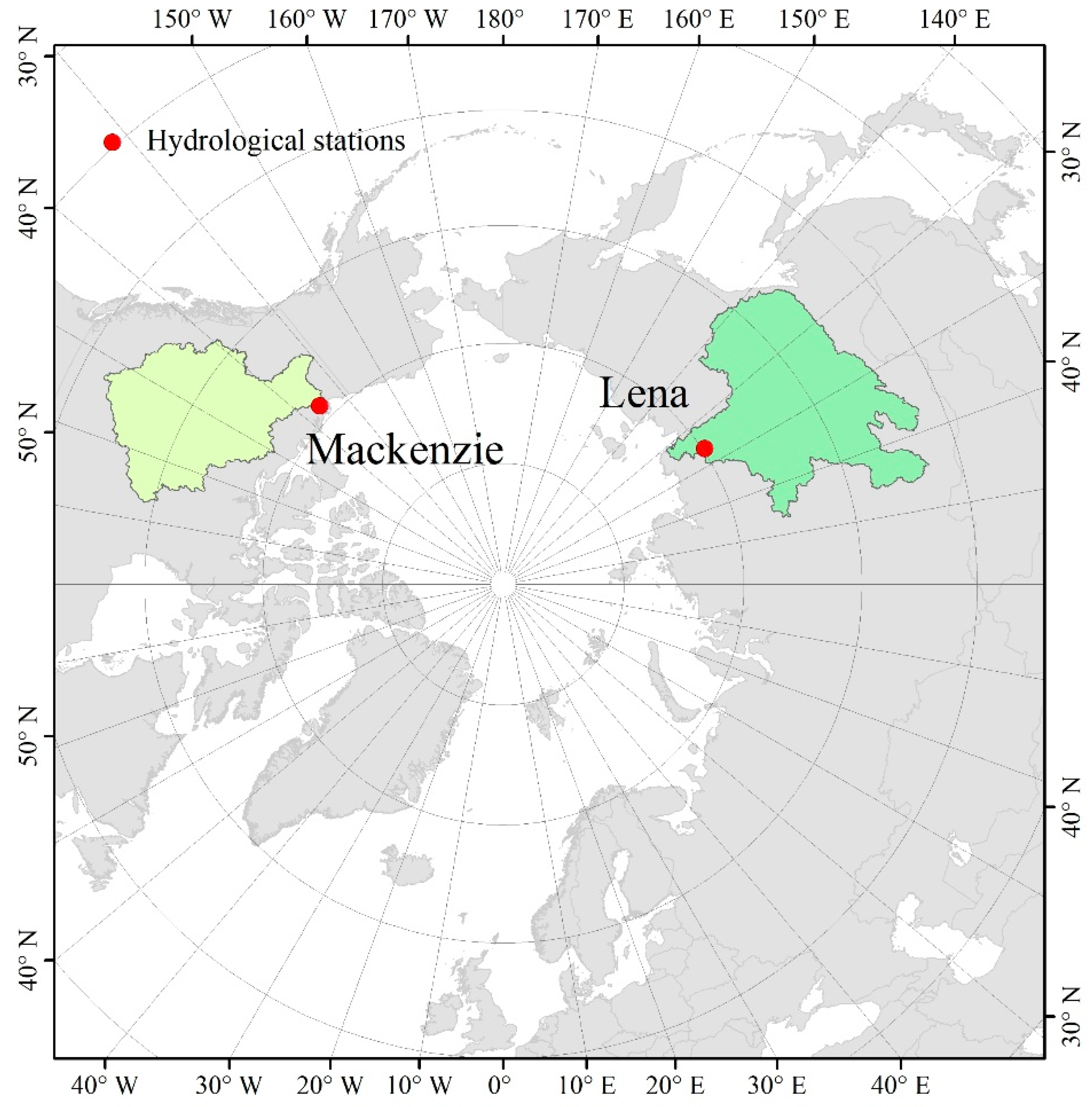
The study areas include the Mackenzie River Basin (MRB) and Lena River Basin (LRB), which are located in North America and Eastern Siberia in the Russian Federation, respectively (Figure 1). The area of the MRB is 180 × 104 km2, which is the largest North American river [42]. Wetland and permafrost cover approximately 49% and 75% in the MRB. The freshwater contribution of the MRB accounts for about 7% of the annual inflow to the Arctic Ocean, and the mean annual discharge is about 325 km3/year [43]. The area of the LRB is 243 × 104 km2, including one of the largest rivers in the Arctic. The mean discharge is 532 km3/year, and freshwater accounts for 15% of the total among flowing into the Arctic Ocean [5,44,45]. The continuous permafrost accounts for 71% in the LRB, and about 78–93% of the basin is covered by permafrost [46,47].
3. Data and Methodology
3.1. Data
3.1.1. Temperature and Precipitation Data
The monthly air temperature and precipitation data were extracted from the high-resolution and long-term gridded dataset of the Global Precipitation Climatology Center (GPCC) (http://climate.geog.udel.edu/~climate/html_pages/download.html#wb_ts2017 (accessed on 16 November 2020)). The GPCC dataset incorporates observations from 75,000 stations worldwide from 1901 to 2017 [48]. The GPCC V7 dataset was based on an enlarged and improved database to reduce the associated uncertainties from the source data, and the systematic gauge measuring error was corrected, which has been widely used to support model climate variability analyses, validations, regional climate monitoring and water resource assessment studies [49,50,51,52]. The V7 version reduced the uncertainty of the dataset using an enlarged and improved database and is expected to include an improved correction of the systematic gauge measuring error [50]. Therefore, the GPCC dataset with the highest spatial resolution (0.5° × 0.5°) was used during 2003–2016. Four seasons, namely the spring (March–May), summer (June–August), autumn (September–November) and winter (December–February), were defined for the seasonal analysis in the current study.
3.1.2. TWS retrieved from GRACE
Data retrieved from the Gravity Recovery and Climate Experiment (GRACE) satellite were used for analyzing the TWS change [3,34,53,54,55]. The GRACE data products were freely downloaded from the GRACE Tellus website (https://grace.jpl.nasa.gov/data/get-data/monthly-mass-grids-land/ (accessed on 17 November 2020)). Preprocessing was conducted to remove noise by filtering and truncation [56,57]. The monthly TWS changes from 2003 to 2016 were used with a spatial resolution of 1° × 1°.
3.1.3. ET Data
The Global Land Evaporation Amsterdam Model (GLEAM) was used to calculate the ET (https://www.gleam.eu/ (accessed on 15 November 2020)) [58]. GLEAM is driven by reanalysis or station-based forcing data (e.g., net radiation and air temperature from ERA-Interim and the Multi-Source Weighted-Ensemble Precipitation data for the ET dataset) and applies a two-step method for estimating the ET, including the traditional method proposed by Priestley and Taylor (1972), followed by a function of the root zone soil moisture and vegetation optical depth. A wide range of water balance-based and EC-based evaluations [25,59] suggested that GLEAM ET data have been demonstrated to be accurate in a variety of ecosystems. Therefore, GLEAM often serves as a reference data for assessing other sorts of large-scale ET data [60]. GLEAM has been used not only in estimating large-scale ET dynamics [61] but also land–atmosphere interactions and drought monitoring [62,63]. In this study, the GLEAM v3.2a ET product during 2003–2016 was used with a spatial resolution of 0.25° × 0.25°.
3.1.4. Runoff Data
In this study, the runoff data was collected by the Arctic Great Rivers Observatory (ArcticGRO, Falmouth, MA, USA) [64] jointly managed by national hydrological institutions in Russia (Roshydromet), the United States (the US Geological Survey; USGS) and Canada (the Water Survey of Canada; WSC) (https://arcticgreatrivers.org/data/ (accessed on 15 November 2020)). The Russian Hydrometeorological Services, which is in charge of the quality control of the discharge data, has conducted systematical observations of discharges in the Siberian region since the late 1930s [44]. The data have been rigorously validated by various hydrological institutions (Arctic and Antarctic Research Institute (AARI), St. Petersburg et al.) [65]. We used the monthly discharge data during 2003–2016 at the Arctic Red River hydrological station of the MRB and Kusur hydrological station of the LRB, respectively. For comparison purposes, we converted the discharge (m3/s) data to the runoff depth (mm).
3.2. Method
3.2.1. Mann–Kendall Test with Trend-Free Pre-Whitening
The Mann–Kendall (MK) test with trend-free pre-whitening (TFPW-MK) has been used in studies of hydrological trend detection. The equations for the MK test method are given below:
where Xi is the value of year i, n is the length of the data and m is the number of groups with tied ranks, each with ti tied observations. If |Z| > Z1−α/2, the null hypothesis is rejected, and the alternative hypothesis is accepted at the significance level of α; otherwise, the null hypothesis of no trend is accepted at the significance level of α.
Trend-free pre-whitening includes the following steps:
where xt is the value of year t of the time series, n is the length of the data and is the average value. The original MK test was applied to Yt to assess the significance of the trend.
3.2.2. Hydrograph Separation
Various methods have been proposed to separate the base flow from the measured total discharge hydrograph. The analysis of the base flow provided valuable insights into understanding the dynamic changes of the groundwater and its contribution to the stream flow under climate changes [66,67]. However, most of the existing methods are rather subjective, which cannot provide consistent and converged results, even with the same input data [68].
Digital filtering algorithms have become powerful tools in hydrograph analyses [68,69,70]. The stream flow is distinguished as a direct runoff and base flow using the digital filter method. The direct runoff indicates a stream flow component changing with a high frequency, including the surface runoff and interflow, while the base flow represents a stream flow component changing with a low frequency, including groundwater discharge and the shallow subsurface flow. A two-parameter digital filtering algorithm is expressed as follows:
where bt is the filtered base flow at time step t; α is the filter parameter; qb−1 is the filtered base flow at time t−1; Qt is the total stream flow at time step t; and BFImax is the maximum value of the long-term ratio of base flow to the total discharge, defined as 0.25 for perennial streams with hard rock aquifers, 0.50 for ephemeral streams with porous aquifers and 0.80 for perennial streams with porous aquifers [69].
The two-parameter digital filter algorithm was validated by comparing the results with measured data in Illinois, Pennsylvania and Maryland [71]. In cold regions, this method also has been successfully applied in river drainage basins with permafrost [72,73]. Therefore, we used the automated digital filter techniques for hydrograph separation in the Arctic regions.
4. Results
4.1. Recent Changes in Temperature and Precipitation
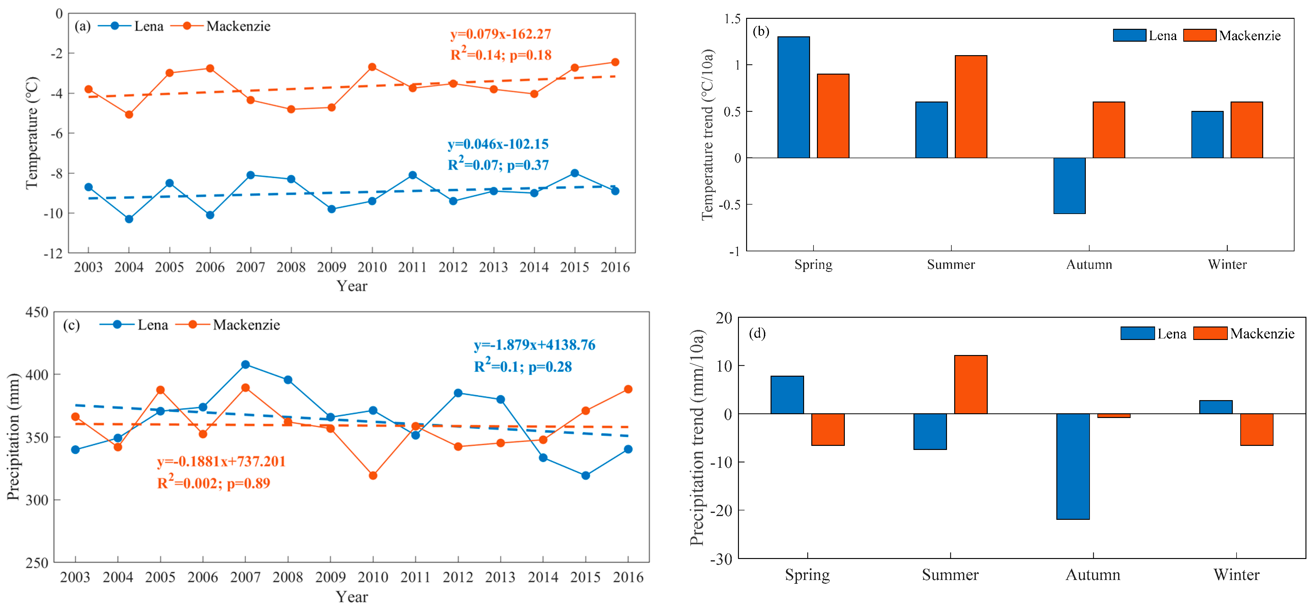
The seasonal and annual variability of the temperatures in the MRB and LRB during 2003–2016 are shown in Figure 2a,b and Table 1. Annually, the temperatures in the two basins showed increased trends (Table 1 and Figure 2a). The warming trends of annual temperatures during the study period were 0.79 °C/10a and 0.46 °C/10a in the MRB and LRB, respectively (Figure 2a). The Arctic amplification was much stronger than the global warming rate 0.19 °C/10a during the last decades. The annual air temperature increased by around 11.06 °C and 6.2 °C during 2003–2016 in MRB and LRB, respectively. The magnitude of the warm trends was more obvious in the MRB of North America than in the LRB of Eastern Siberia. The temperatures in the MRB showed increasing trends in all the seasons (Figure 2b and Table 1). The rates of the temperatures were stronger in the spring and summer than in the autumn and winter. The temperature in the LRB showed an increasing trend in the spring, summer and winter, while it had a decreased trend in the autumn (Figure 2b and Table 1). The results showed obvious warming during the past 14 years over the entire study area.
The seasonal and annual variabilities of the precipitation in the MRB and LRB during 2003–2016 are shown in Figure 2c,d and Table 1. Annually, the precipitation in LRB had a significantly decreased trend and that in MRB showed a nonsignificantly decreased trend (Table 1 and Figure 2c). The mean annual precipitations were 359.2 mm and 363.1 mm in the MRB and LRB, respectively. The annual precipitations had decreased rates of 1.9 mm/10a and 18.8 mm/10a in the MRB and LRB, respectively (Figure 2c), which were unlike the positive trends in global surface temperatures over the past century. The changes of precipitation in the study basins were different with the trends in global precipitation, which showed no significant changes based on the GPCP dataset [74]. The annual precipitation increased during 2003–2006 but started to decline after 2000 in the LRB, while the precipitation increased after 2010 in the MRB. Except for the summer, the precipitations decreased in the spring, autumn and winter in the MRB, which were 60.1 mm,150.6 mm, 89.6 mm and 58.9 mm in the spring, summer, autumn and winter, respectively (Table 1 and Figure 2d). In the LRB, the spring and winter precipitations showed increased trends, while they showed decreased trends in the summer and autumn, and the precipitations were 57.0 mm, 177.3 mm, 94.6 mm and 34.2 mm in the spring, summer, autumn and winter, respectively. From the magnitudes of the decreases in the relevant seasons, it can be seen that the decrease of annual precipitation in the LRB was mainly due to the decreased precipitation in the autumn.
4.2. Changes in ET
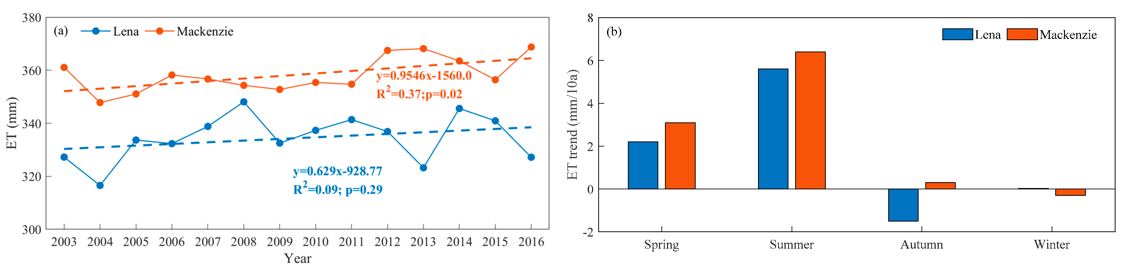
The mean annual ET in the MRB and LRB were 358.3 mm and 334.4 mm, respectively, which were almost equal to the amount of precipitation. The annual ET series in the MRB had a significantly increased trend and that in LRB showed a nonsignificantly increased trend (Table 2 and Figure 3a). The ET in the two basins experienced increases of 9.5 and 6.3 mm/10a during 2003–2016, respectively (Figure 3a). Seasonally, ET showed an increasing trend in the spring and summer in two basins, and the greatest increase appeared in the summer, with rates of 64 mm/a and 56 mm/a, respectively (Figure 3b and Table 2). The decreased trend occurred in the autumn of the LRB and in the winter of the MRB (Figure 3b and Table 2). The area average magnitudes of ET were 102.2 mm, 224.7 mm, 29.7 mm and 1.6 mm for the spring, summer, autumn and winter in the MRB. The area average magnitudes of ET were 93.8 mm, 214.8 mm, 25.5 mm and 0.4 mm for the spring, summer, autumn and winter in the LRB.
4.3. Changes in TWS
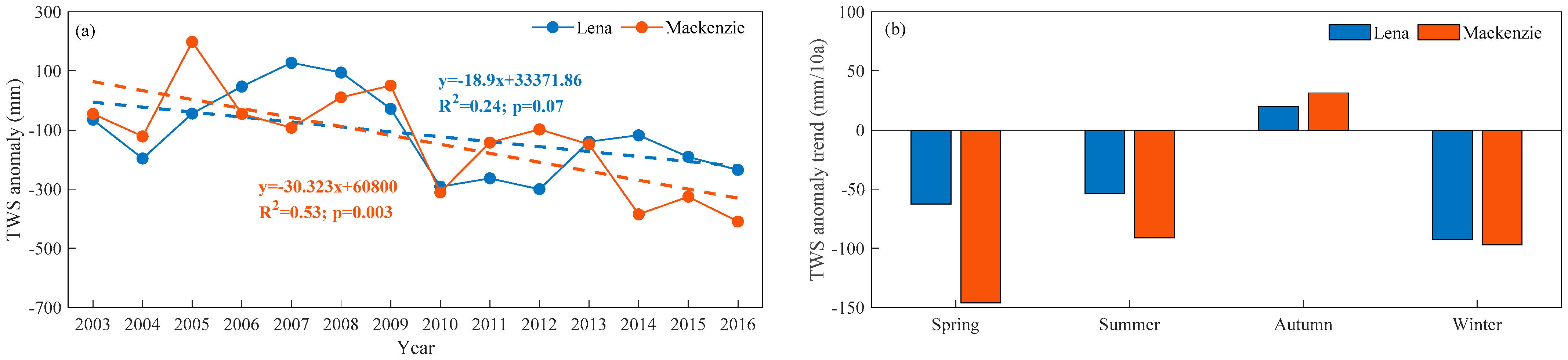
TWS anomalies in the GRACE dataset showed significantly decreased trends during 2003–2016 in the MRB and LRB, with declines of 30.3 mm/a and 18.9 mm/a (Figure 4a and Table 3). The variations indicate more freshwater flowing out of two basins, which showed a state of deficit. The maximum positive anomalies of TWS were 127.3 mm and 198.2 mm in the LRB and MRB, respectively, occurring in 2007 and 2005. The minimum negative anomalies of −300.3 mm and −409.4 mm in the LRB and MRB, respectively, occurred in 2012 and 2016. The seasonal analysis results indicated that the seasonal variations in the TWS were consistent between the two basins during 2003–2016. Figure 4b and Table 3 show that the TWS in the LRB and MRB had negative anomalies in the spring, summer and winter and a positive trend in the autumn. The greatest decrease occurred in the spring in the MRB, while it occurred in the winter in the LRB. The state of the seasonal deficit was stronger in the MRB than in the LRB, while the state of gain was stronger in the LRB than in the MRB. The results indicated that more water was released in the MRB and LRB in the spring, summer and winter and stored in the autumn.
4.4. Changes in Runoff
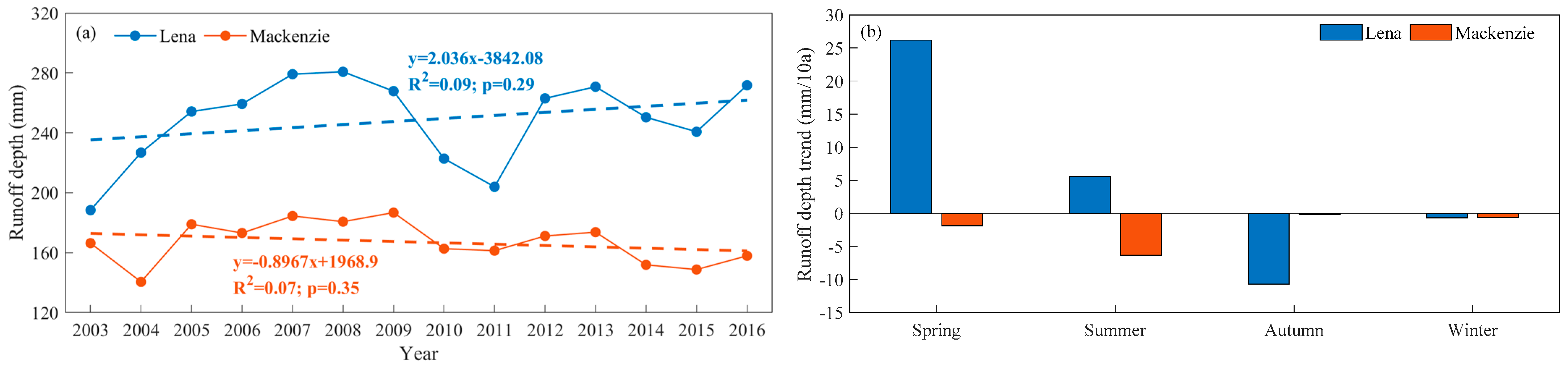
The annual runoff showed obvious changes during 2003–2016 and experienced an upward trend with a rate of 2.0 mm/a in the LRB (Figure 5a and Table 4). A rapid increase in the annual runoff occurred before 2008, when the TWS also showed a significant increase. In the MRB, the runoff showed a slight decreased trend with a rate of −0.9 mm/a (Figure 5a and Table 4). The mean annual runoff depths were 167.0 mm and 248.6 mm in the MRB and LRB, respectively. The runoffs in the spring and summer increased in the LRB, while it significantly decreased in the autumn and winter (Figure 5b and Table 4). The spring runoff increased in the Siberian regions primarily due to climate warming during snowmelt periods associated with early snowmelts [75,76,77,78]. The maximum and minimum magnitudes of the trends occurred in the spring and autumn in the LRB, respectively, with rates of 26.2 mm/10a and −10.7 mm/10a. The runoff depths in the spring, summer, autumn and winter were 27.5 mm, 149.9 mm, 57.5 mm and 13.7 mm in the LRB. In the MRB, the runoff decreased in all the seasons, and the minimum trend was in the summer with a rate of −6.3 mm/10a (Figure 5b and Table 4). The runoff depths in the spring, summer, autumn and winter were 34.7 mm, 74.6 mm, 39.5 mm and 18.2 mm.
5. Discussion
5.1. The Impacts of Precipitation, Temperature and TWS on the Stream Flow
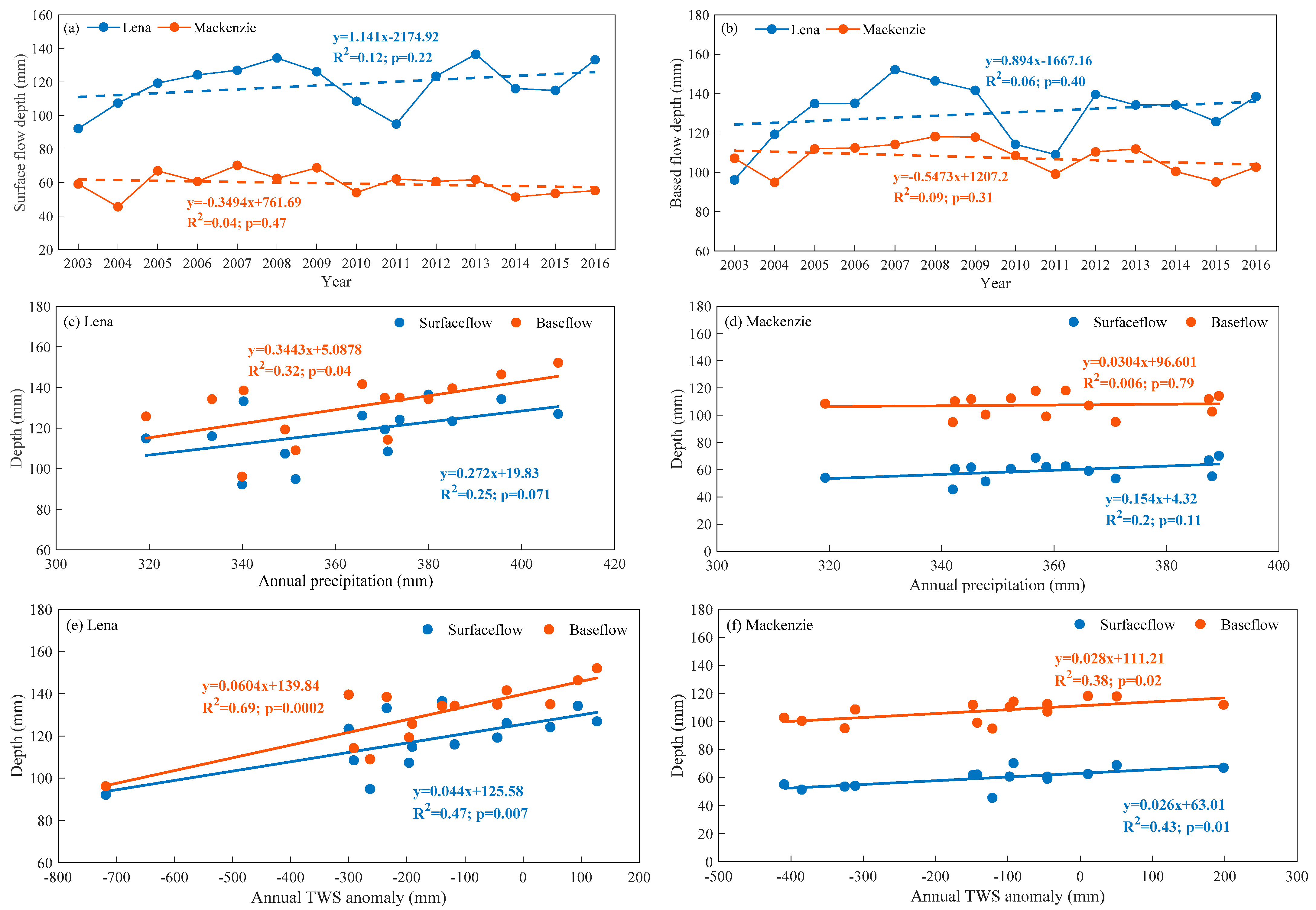
Figure 6a,b showed the hydrological separation in two basins from 2003 to 2016 calculated by Equation (8). The annual surface flow and base flow showed increased trends in the LRB, whereas both showed a decreased trend in the MRB. The surface flow and base flow contributed 56% and 44% to the increased total runoff in the LRB, and the surface flow impacted stronger on the runoff than the base flow. In the MRB, the surface flow and base flow contributed to a 39% and 61% decrease in the total runoff, and the decreased runoff was mainly influenced by the base flow. The annual TWS anomalies were more highly related to the surface flow and base flow than precipitation in the LRB (Figure 6c,e). The annual precipitation and TWS showed a significantly decreased trend during 2003–2016, with more TWS released the same as the runoff. Therefore, the increased annual runoff in this area was mainly attributed to the TWS increase. In the MRB, the correlation coefficient between annual precipitation and surface flow was 0.45, and changes in the annual TWS showed stronger relationships with the surface flow and base flow, which were 0.66 and 0.62, respectively. Both annual precipitation and TWS showed decreased trends, suggesting the control of the annual precipitation and TWS on the interannual variability in the runoff.
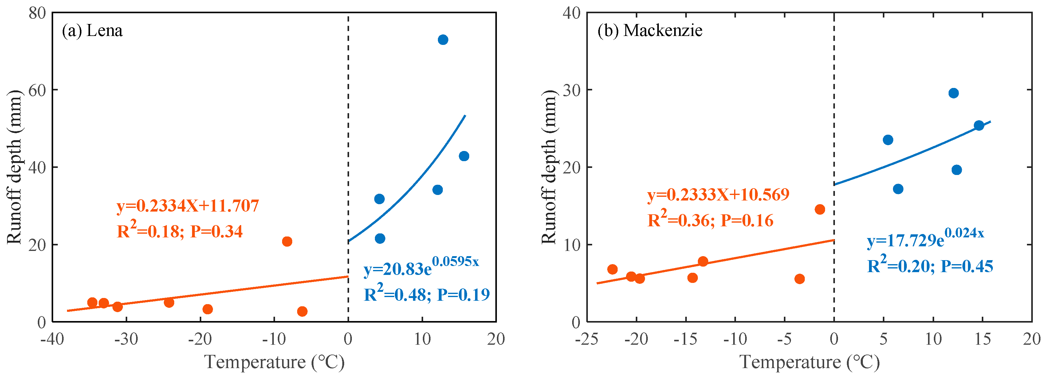
Temperature is an important factor that affects the changes of runoffs in the Arctic region. The relationship between temperature and runoff is shown in Figure 7. The temperature influence on the runoff was comparatively less at temperatures less than 0 °C in the MRB and Lena (Figure 7a,b). The increased rate of the runoff depth was 0.23 mm/°C in the two basins. This may be because the runoff was generated from the base flow. Previous studies have shown that the snow depth and runoff during the spring showed significant correlations in Arctic rivers [42]. At temperatures above 0 °C, the runoff increased dramatically as snowmelt (Figure 7a,b). In this case, the snowmelt water increased with the increase in temperature. The increased rate of runoff depth in Lena was higher than that in Mackenzie.
5.2. Seasonal Cycles of Hydrological Components
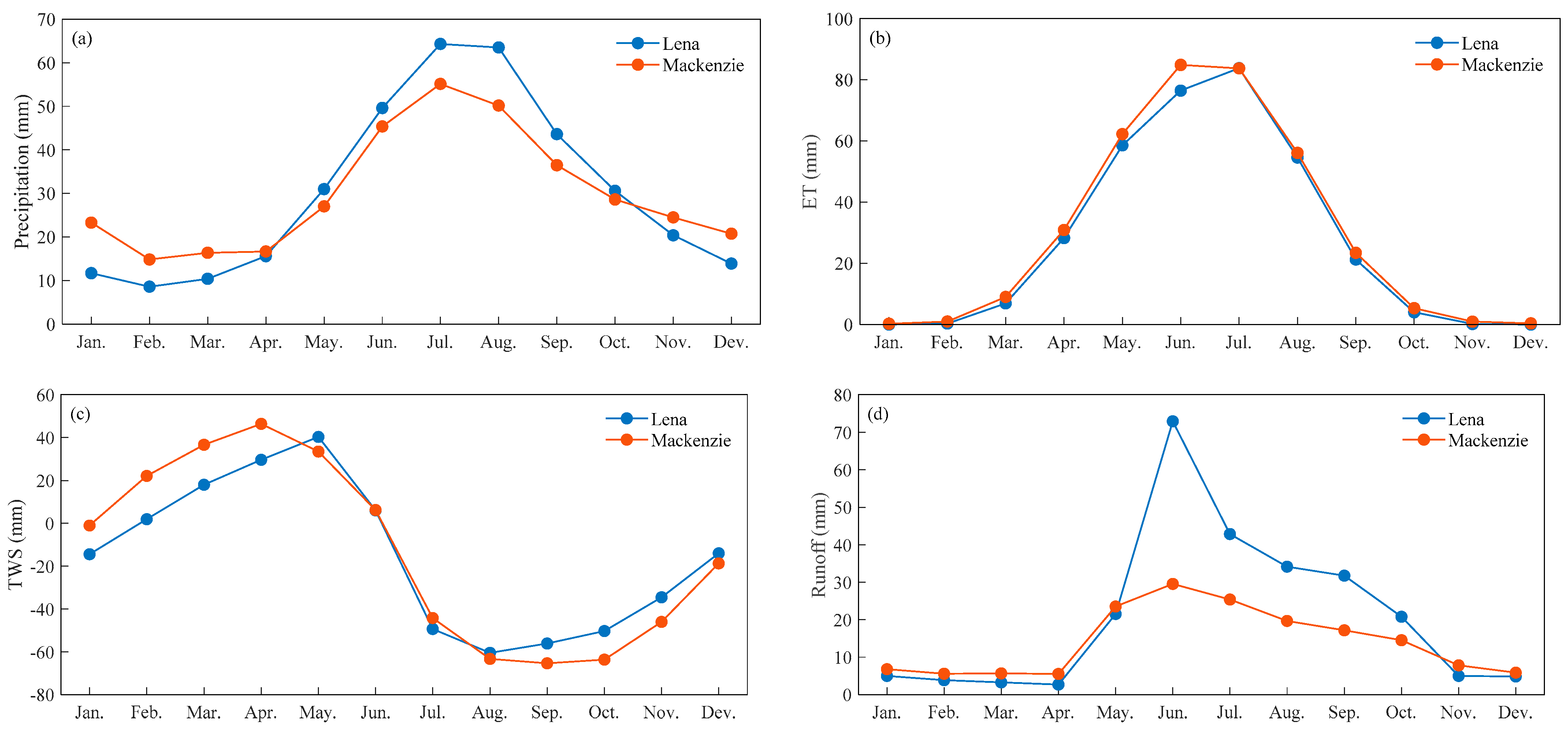
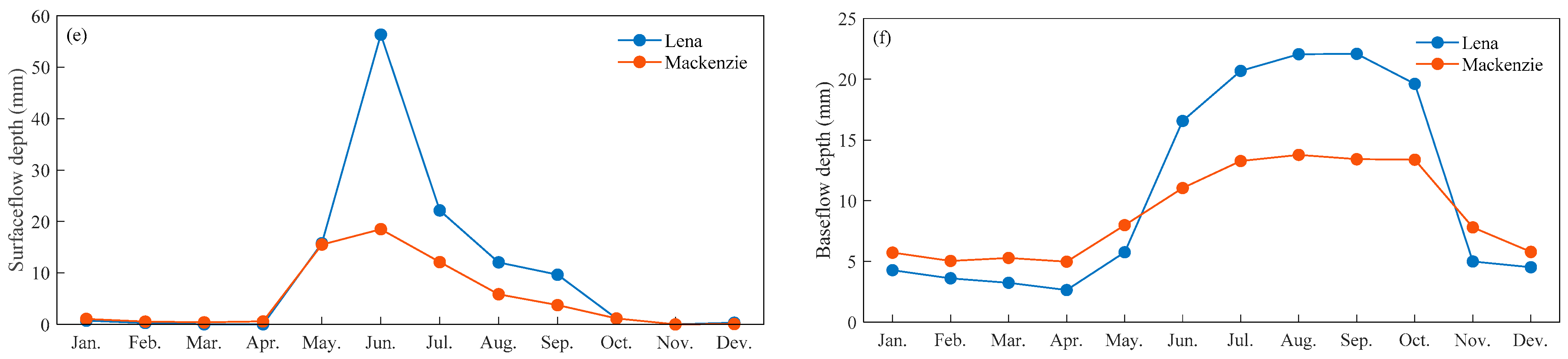
As shown in Figure 8, the trends of the precipitation and ET agreed relatively well in the LRB and MRB, both peaking around June–August and reaching a minimum between November and February. The precipitation from November to March was higher in the MRB than in the LRB. However, it was lower from May to October. The ET was higher in the MRB than in the LRB. The TWS showed positive anomalies from February to June and negative anomalies from July to January in the two basins. As seen, the runoff remained high during May–October and then decreased to reach the annual low in April before increasing again throughout the second half of the year. The positive anomaly of the TWS was caused by the accumulation of snow, low ET and runoff. It is evident that winter precipitation significantly influenced the hydrological cycle in the MRB and LRB. The surface flow was concentrated from May to September, and the differences between the high runoff and low runoff were obviously mainly due to the snowmelt [77,79]. The base flow from November to May was higher in the MRB than in the LRB, and it was obviously higher from June to October in the LRB. The maximum base flow occurred in August and September, which lagged 2 to 3 months compared to the surface flow. In the Arctic region, the permafrost conditions also highly influenced the hydrological regime; basins with more permafrost coverage (such as LRB) had lower subsurface storage capacity and, thus, a lower winter base flow and a higher summer peak flow [80,81,82].
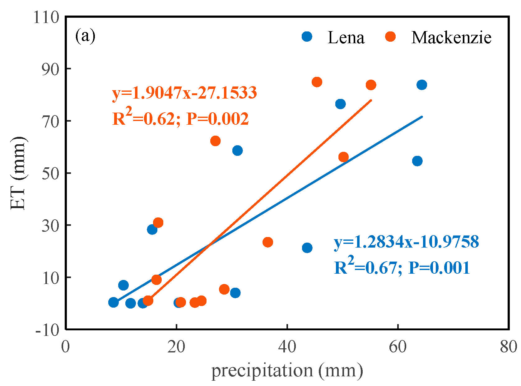
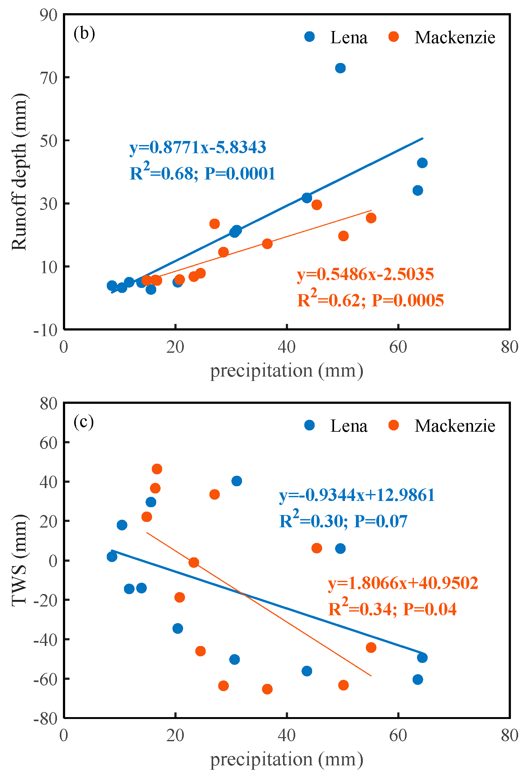
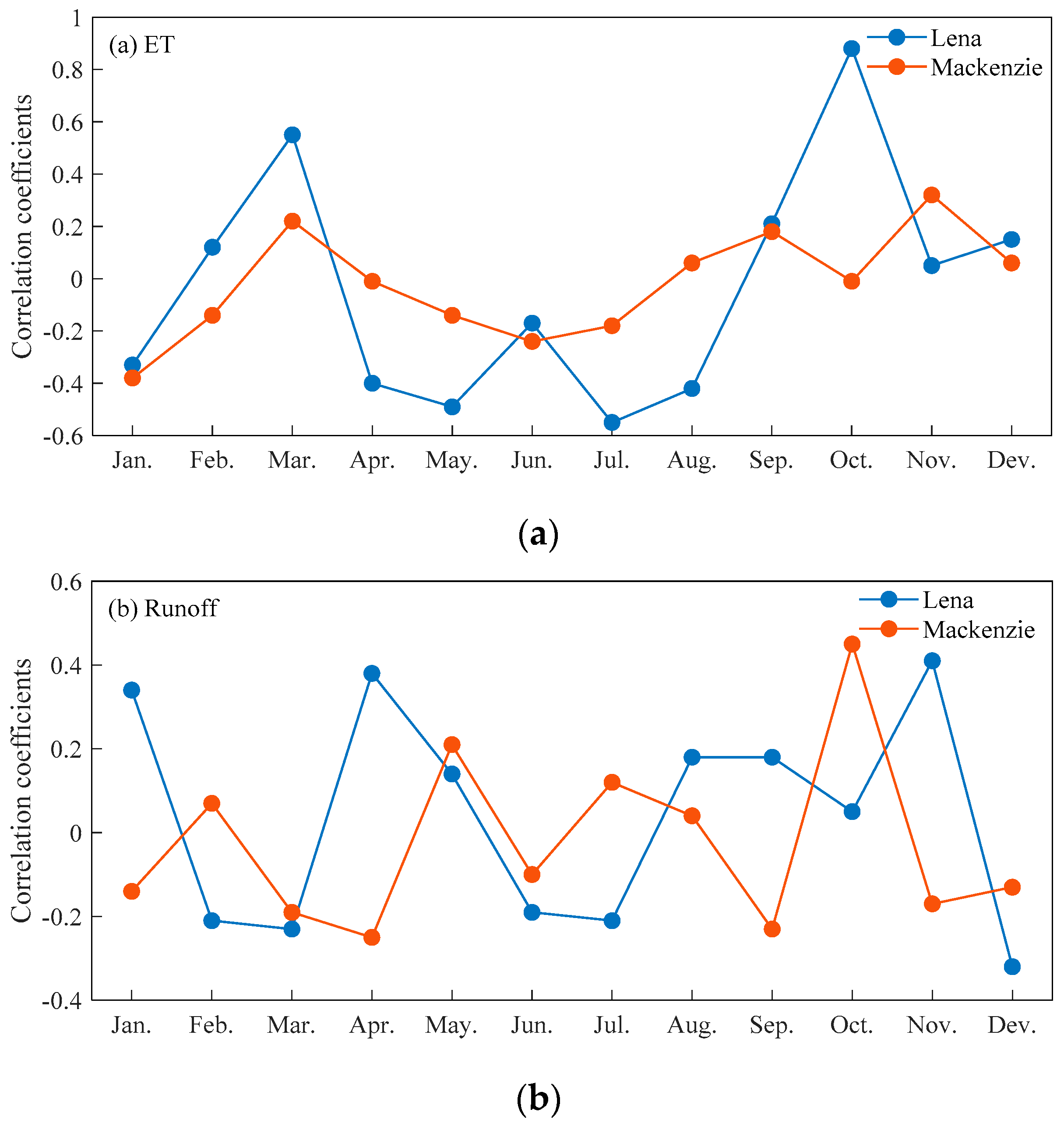
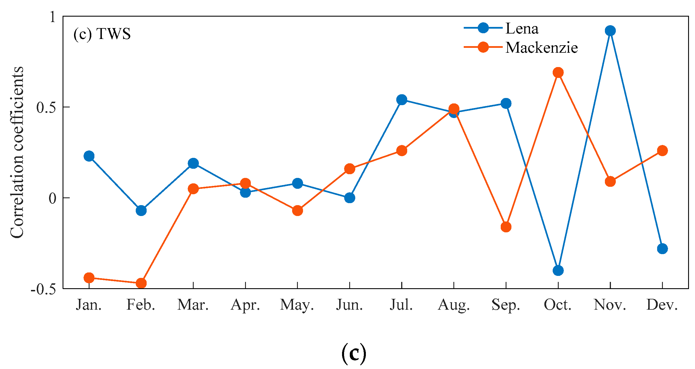
Precipitation had a positive correlation with the ET and runoff in general (Figure 9a,b). The relationships between monthly precipitation and ET were better correlated in the LRB (R = 0.82, p = 0.001) than in the MRB (R = 0.79, p = 0.002) (Figure 9a). However, there were also phase differences for different months. There were higher positive relationships in March and October and high negative relationships in May and July (Figure 10a). The relationships between the monthly precipitation and runoff were also better correlated in the LRB (R = 0.82, p = 0.0001) than in the MRB (R = 0.79, p = 0.0005) (Figure 9b). The monthly precipitation more highly positively influenced by the monthly runoff mainly occurring in January, April and November in the LRB, and it occurred only in October in the MRB, which indicated that the runoff was influenced by precipitation (Figure 10b). For the TWS, there were negative correlation with precipitation in general (Figure 9c). The relationships between the monthly precipitation and TWS were better correlated in the MRB (R = 0.58, p = 0.04) than in the LRB (R = 0.55, p = 0.07) (Figure 9c). In the MRB, the monthly precipitation showed higher negative relationships in January and February, whereas they showed higher positive relationships in August and October (Figure 10c). The positive relationships between monthly precipitation and TWS were higher in July, August, September and November in the LRB, suggesting that the precipitation impacted on the TWS (Figure 10c). Overall, the impact of the precipitation on the ET, runoff and TWS on a monthly scale showed huge differences in the different river basins over the Arctic region.
5.3. Telationship between Precipitation and Other Hydrological Components
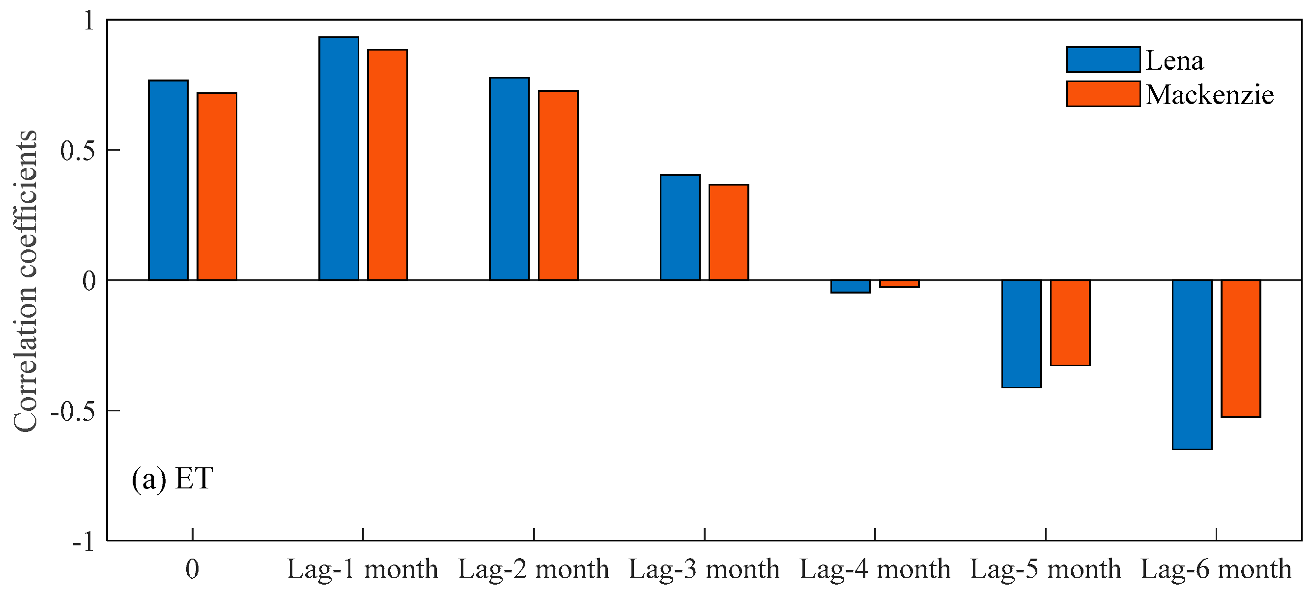
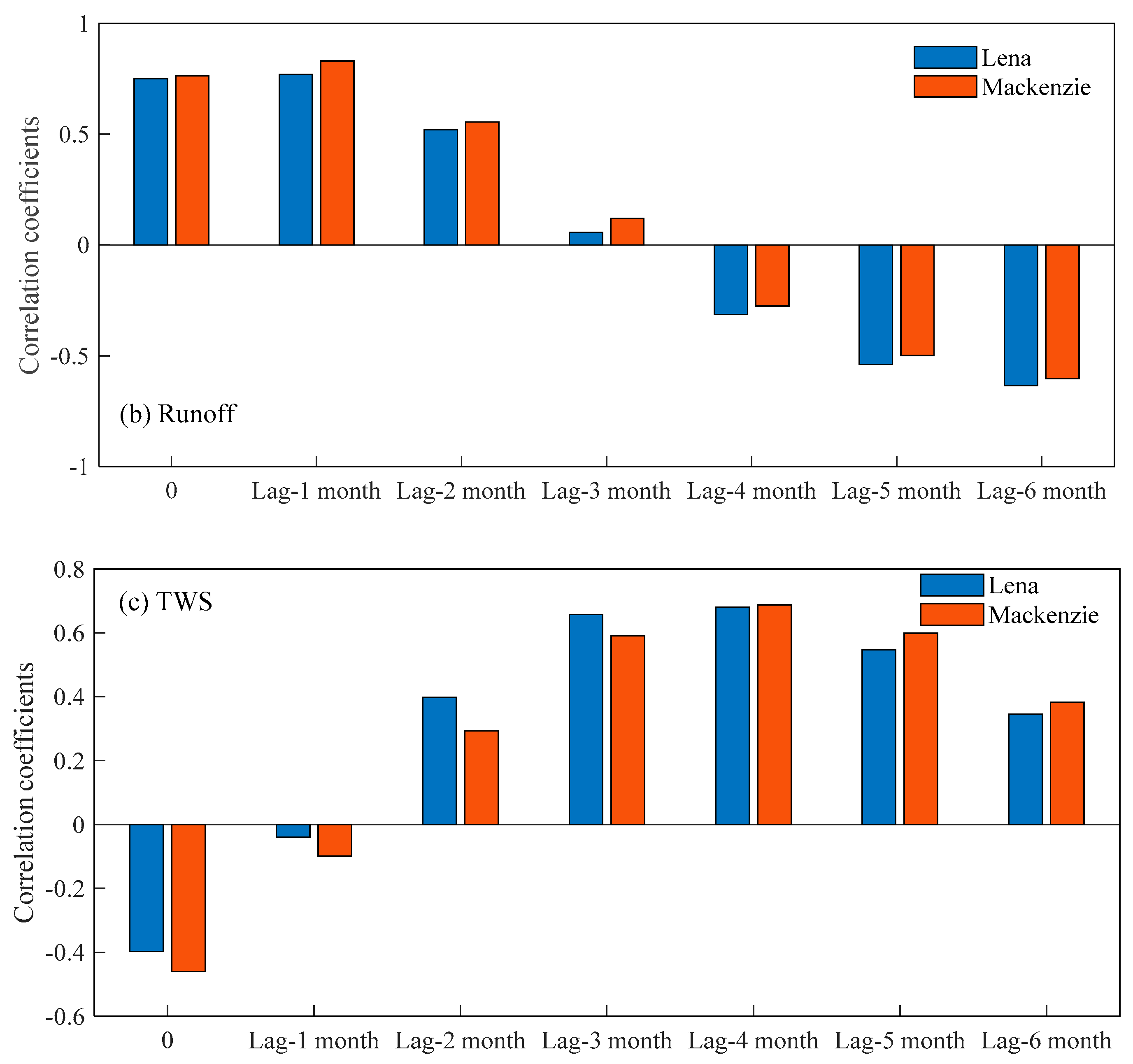
As the key component and driving factor in the hydrologic cycle, precipitation has a prominent influence on the interactions among other hydrologic components [83]. There is a lag time from when water is introduced as the precipitation compared to when it becomes surface water, ET and TWS, which is typically described empirically as the total precipitation in the hydrological balance [84]. The time lags of the ET, runoff and TWS responses to precipitation are shown in Figure 11. The results indicated that the ET and runoff were most highly related to precipitation over a 1-month lag, i.e., the monthly ET and runoff were strongly influenced by the precipitation that occurred 1 month earlier in the study area. The negative relationships between precipitation and ET and runoff occurred after a lag of 4 months, and the maximum negative relationships both occurred after a 6-month time lag. The monthly precipitation and the TWS were negatively correlated without any lag and poorly negatively correlated over a 1-month lag. As time goes by, the relationships between precipitation and TWS converted from negative values to positive values in the study areas. The TWS were most highly related to precipitation over a time lag of 4 months in the two basins. These results suggested that more precipitation would lead to more TWS when precipitation preceded the TWS by 4 months; in contrast, it would result in less TWS when precipitation preceded it by 0 to 1 month. It is also found that the monthly precipitation mainly formed ET and runoff over the next 3 months; after that, the ET and runoff would gradually decrease, and more precipitation was stored in the basins, which induced the TWS increase in the LRB and MRB.
6. Conclusions
In this study, the changes of the hydrological components in two representative river basins in the Arctic region, namely the Mackenzie River Basin (MRB) and the Lena River Basin (LRB), were investigated using multiple satellite remote sensing and observational datasets during 2003–2016. The main conclusions were as follows:
(1) The changes of the hydrological components in the different basins of Arctic region showed different trends. The annual precipitation decreased at rates of 1.9 mm/10a and 18.8 mm/10a in the MRB and LRB, respectively, which was much greater in Eastern Siberia than in North America. The magnitude of the warm trends was obviously more in the MRB of North America than the LRB of Eastern Siberia, which were 0.79 °C/10a and 0.44 °C/10a, respectively. The ET increased more rapidly in the MRB than in the LRB, with rates of 9.5 and 6.3 mm/10, respectively.
(2) The TWS showed a decreased trend during 2003–2016 in the MRB and LRB, with declines of 30.3 mm/a and 18.9 mm/a. The change trends of the runoffs were different with the TWS in the study area. The surface flow and base flow contributed 56% and 44% of the increased total runoff in the LRB. In the MRB, the surface flow and base flow contributed 39% and 61% of the decreased total runoff, so the decreased runoff was mainly influenced by the base flow. The increased annual runoff in the LRB was mainly attributed to a lower ET and less of a deficit of TWS, while a higher ET and more of a deficit of TWS in the MRB controlled the variability in the runoff.
(3) The mean annual cycles of precipitation, ET, TWS, runoff depth, surface flow and base flow in the LRB and MRB showed deviations in the magnitudes and distributions. The precipitation on a monthly scale influenced the ET, runoff and TWS and showed huge differences in the different river basins over Arctic region. There were obviously lag times from rainfall to surface water, ET and TWS in the study areas. The monthly precipitations mainly formed the ET and runoff for the next 3 months; after that, the ET and runoff would gradually decrease, and more precipitation was stored in the basins, which induced TWS increase in the LRB and MRB.
Author Contributions
All authors have contributed equally in methodology and formal analysis. All authors have read and agreed to the published version of the manuscript.
Funding
This research was funded by the National Key Research and Development Program of China (Grant No. 2020YFA0608504), Key CAS Research Program of Frontier Sciences (QYZDY-SSW-DQC021), the project of State Key Laboratory of Cryospheric Science (SKLCS-ZZ-2020, SKLCS-OP-2020–11), Youth Innovation Promotion Association CAS (2019414) and Jiangsu Provincial Double-Innovation Doctor Program.
Institutional Review Board Statement
Not applicable.
Informed Consent Statement
Not applicable.
Data Availability Statement
Not applicable.
Conflicts of Interest
The authors declare no conflict of interest.
References
- Wang, H.; Jia, L.; Steffen, H.; Wu, P.; Jiang, L.; Hsu, H.; Xiang, L.; Wang, Z.; Hu, B. Increased water storage in North America and Scandinavia from GRACE gravity data. Nat. Geosci. 2012, 6, 38–42. [Google Scholar] [CrossRef]
- Van Dijk, A.I.J.M.; Renzullo, L.J.; Wada, Y.; Tregoning, P. A global water cycle reanalysis (2003–2012) merging satellite gra-vimetry and altimetry observations with a hydrological multi-model ensemble. Hydrol. Earth Sys. Sci. 2014, 18, 2955–2973. [Google Scholar] [CrossRef] [Green Version]
- Deng, H.; Chen, Y. Influences of recent climate change and human activities on water storage variations in Central Asia. J. Hydrol. 2017, 544, 46–57. [Google Scholar] [CrossRef]
- Chen, H.; Zhang, W.; Nie, N.; Guo, Y. Long-term groundwater storage variations estimated in the Songhua River Basin by using GRACE products, land surface models, and in-situ observations. Sci. Total. Environ. 2019, 649, 372–387. [Google Scholar] [CrossRef]
- Berezovskaya, S.; Yang, D.; Kane, D.L. Compatibility analysis of precipitation and runoff trends over the large Siberian watersheds. Geophys. Res. Lett. 2004, 31, L21502. [Google Scholar] [CrossRef] [Green Version]
- Serreze, M.C.; Barrett, A.P.; Slater, A.; Woodgate, R.A.; Aagaard, K.; Lammers, R.B.; Steele, M.; Moritz, R.; Meredith, M.; Lee, C.M. The large-scale freshwater cycle of the Arctic. J. Geophys. Res. Space Phys. 2006, 111, C110. [Google Scholar] [CrossRef] [Green Version]
- Bring, A.; Fedorova, I.; Dibike, Y.; Hinzman, L.; Mård, J.; Mernild, S.H.; Prowse, T.; Semenova, O.; Stuefer, S.; Woo, M. Arctic terrestrial hydrology: A synthesis of processes, regional effects, and research challenges. J. Geophys. Res. Biogeosci. 2016, 121, 621–649. [Google Scholar] [CrossRef]
- Holmes, R.M.; Coe, M.T.; Fiske, G.J.; Gurtovaya, T.; Zhulidov, A.V. Climate Change Impacts on the Hydrology and Biogeochemistry of Arctic Rivers. Climatic Change and Global Warming of Inland Waters: Impacts and Mitigation for Ecosystems and Societies; John Wiley & Sons, Ltd.: Hoboken, NJ, USA, 2012. [Google Scholar]
- Xu, M.; Kang, S.; Wang, X.; Wu, H.; Hu, D.; Yang, D. Climate and hydrological changes in the Ob River Basin during 1936–2017. Hydrol. Process. 2020, 34, 1821–1836. [Google Scholar] [CrossRef]
- Serreze, M.C.; Walsh, J.; Iii, F.S.C.; Osterkamp, T.; Dyurgerov, M.; Romanovsky, V.; Oechel, W.; Morison, J.; Zhang, T.; Barry, R. Observational Evidence of Recent Change in the Northern High-Latitude Environment. Clim. Chang. 2000, 46, 159–207. [Google Scholar] [CrossRef]
- Arctic Climate Impact Assessment. Arctic Climate Impact Assessment Overview Report; Cambridge University Press: New York, NY, USA, 2005. [Google Scholar]
- Sheffield, J.; Ferguson, C.R.; Troy, T.; Wood, E.; McCabe, M. Closing the terrestrial water budget from satellite remote sensing. Geophys. Res. Lett. 2009, 36, L07403. [Google Scholar] [CrossRef]
- Sahoo, A.K.; Pan, M.; Troy, T.J.; Vinukollu, R.K.; Sheffield, J.; Wood, A.E.F. Reconciling the global terrestrial water budget using satellite remote sensing. Remote Sens. Environ. 2011, 115, 1850–1865. [Google Scholar] [CrossRef]
- Reichert, J.M.; Rodrigues, M.F.; Peláez, J.J.Z.; Lanza, R.; Minella, J.P.G.; Arnold, J.G.; Cavalcante, R.B.L. Water balance in paired watersheds with eucalyptus and degraded grassland in Pampa biome. Agric. For. Meteorol. 2017, 237–238, 282–295. [Google Scholar] [CrossRef]
- Wu, P.; Wood, R.; Stott, P. Human influence on increasing Arctic River discharges. Geophys. Res. Lett. 2005, 32, L02703. [Google Scholar] [CrossRef]
- Curtis, J.; Wendler, G.; Stone, R.; Dutton, E. Precipitation decrease in the western Arctic, with special emphasis on Barrow and Barter Island, Alaska. Int. J. Clim. 1998, 18, 1687–1707. [Google Scholar] [CrossRef]
- Przybylak, R. Variability of total and solid precipitation in the Canadian Arctic from 1950 to 1995. Int. J. Clim. 2002, 22, 395–420. [Google Scholar] [CrossRef]
- Serreze, M.C.; Etringer, A.J. Precipitation characteristics of the Eurasian Arctic drainage system. Int. J. Clim. 2003, 23, 1267–1291. [Google Scholar] [CrossRef]
- Houghton, J.T.; Ding, Y.; Griggs, D.J.; Noguer, M.; van der Linden, P.J.; Xiaosu, D. Climate Change 2001: The Scientific Basis; Cambridge University Press: Cambridge, UK, 2001. [Google Scholar]
- Landerer, F.W.; Dickey, J.O.; Güntner, A. Terrestrial water budget of the Eurasian pan-Arctic from GRACE satellite measurements during 2003–2009. J. Geophys. Res. Space Phys. 2010, 115, D23115. [Google Scholar] [CrossRef] [Green Version]
- Peterson, B.J.; Holmes, R.M.; McClelland, J.; Vörösmarty, C.J.; Lammers, R.B.; Shiklomanov, A.I.; Shiklomanov, I.A.; Rahmstorf, S. Increasing River Discharge to the Arctic Ocean. Science 2002, 298, 2171–2173. [Google Scholar] [CrossRef] [Green Version]
- Yang, D.; Shi, X.; Marsh, P. Variability and extreme of Mackenzie River daily discharge during 1973–2011. Quat. Int. 2015, 380–381, 159–168. [Google Scholar] [CrossRef]
- Déry, S.J.; Wood, E.F. Decreasing river discharge in Northern Canada. Geophys. Res. Lett. 2005, 32, L10401. [Google Scholar] [CrossRef] [Green Version]
- Fisher, J.B.; Melton, F.; Middleton, E.; Hain, C.; Anderson, M.; Allen, R.; McCabe, M.F.; Hook, S.; Baldocchi, D.; Townsend, P.A.; et al. The future of evapotranspiration: Global requirements for ecosystem functioning, carbon and climate feedbacks, agricultural management, and water resources. Water Resour. Res. 2017, 53, 2618–2626. [Google Scholar] [CrossRef]
- Ma, N.; Szilagyi, J. The CR of Evaporation: A Calibration-Free Diagnostic and Benchmarking Tool for Large-Scale Terrestrial Evapotranspiration Modeling. Water Resour. Res. 2019, 55, 7246–7274. [Google Scholar] [CrossRef] [Green Version]
- Baldocchi, D.D.; Falge, E.; Gu, L.R.; Olson, D. FLUXNET: A New Tool to Study the Temporal and Spatial Variability of Ecosystem-Scale Carbon Dioxide, Water Vapor and Energy Flux Densities. B. Am. Meteorol. Soc. 2001, 82, 2415–2435. [Google Scholar] [CrossRef]
- Ma, N.; Szilagyi, J.; Zhang, Y.; Liu, W. Complementary-Relationship-Based Modeling of Terrestrial Evapotranspiration Across China During 1982–2012: Validations and Spatiotemporal Analyses. J. Geophys. Res. Atmos. 2019, 124, 4326–4351. [Google Scholar] [CrossRef]
- Wang, K.; Dickinson, R.E. A review of global terrestrial evapotranspiration: Observation, modeling, climatology, and climatic variability. Rev. Geophys. 2012, 50, RG2005. [Google Scholar] [CrossRef]
- Dankers, R.; Christensen, O.B. Climate Change Impact on Snow Coverage, Evaporation and River Discharge in the Sub-Arctic Tana Basin, Northern Fennoscandia. Clim. Chang. 2005, 69, 367–392. [Google Scholar] [CrossRef]
- Suzuki, K.; Matsuo, K.; Hiyama, T. Satellite gravimetry-based analysis of terrestrial water storage and its relationship with run-off from the Lena River in eastern Siberia. Int. J. Remote Sens. 2016, 37, 2198–2210. [Google Scholar] [CrossRef] [Green Version]
- Iijima, Y.; Fedorov, A.N.; Park, H.; Suzuki, K.; Yabuki, H.; Maximov, T.C.; Ohata, T. Abrupt increases in soil temperatures following increased precipitation in a permafrost region, central Lena River basin, Russia. Permafr. Periglac. Process. 2010, 21, 30–41. [Google Scholar] [CrossRef]
- Walvoord, M.A.; Kurylyk, B.L. Hydrologic Impacts of Thawing Permafrost—A Review. Vadose Zone J. 2016, 15, 1–20. [Google Scholar] [CrossRef]
- Xu, M.; Kang, S.; Chen, X.; Wu, H.; Wang, X.; Su, Z. Detection of hydrological variations and their impacts on vegetation from multiple satellite observations in the Three-River Source Region of the Tibetan Plateau. Sci. Total. Environ. 2018, 639, 1220–1232. [Google Scholar] [CrossRef]
- Rodell, M.; Famiglietti, J.S.; Chen, J.; Seneviratne, S.I.; Viterbo, P.; Holl, S.; Wilson, C.R. Basin scale estimates of evapotranspiration using GRACE and other observations. Geophys. Res. Lett. 2004, 31, 10–13. [Google Scholar] [CrossRef] [Green Version]
- Rodell, M.; McWilliams, E.B.; Famiglietti, J.S.; Beaudoing, H.K.; Nigro, J. Estimating evapotranspiration using an observation based terrestrial water budget. Hydrol. Process. 2011, 25, 4082–4092. [Google Scholar] [CrossRef]
- Long, D.; Chen, X.; Scanlon, B.R.; Wada, Y.; Hong, Y.; Singh, V.P.; Chen, Y.; Wang, C.; Han, Z.; Yang, W. Have GRACE satellites overestimated groundwater depletion in the Northwest India Aquifer? Sci. Rep. 2016, 6, 24398. [Google Scholar] [CrossRef] [PubMed]
- Long, D.; Pan, Y.; Zhou, J.; Chen, Y.; Hou, X.; Hong, Y.; Scanlon, B.R.; Longuevergne, L. Global analysis of spatiotemporal variability in merged total water storage changes using multiple GRACE products and global hydrological models. Remote Sens. Environ. 2017, 192, 198–216. [Google Scholar] [CrossRef]
- Swann, A.L.S.; Koven, C.D. A Direct Estimate of the Seasonal Cycle of Evapotranspiration over the Amazon Basin. J. Hydrometeorol. 2017, 18, 2173–2185. [Google Scholar] [CrossRef] [Green Version]
- Pan, M.; Wood, E.; Wojcik, R.; McCabe, M. Estimation of regional terrestrial water cycle using multi-sensor remote sensing observations and data assimilation. Remote Sens. Environ. 2008, 112, 1282–1294. [Google Scholar] [CrossRef]
- Sheffield, J.; Wood, E.; Roderick, M. Little change in global drought over the past 60 years. Nature 2012, 491, 435–438. [Google Scholar] [CrossRef]
- Kazuyoshi, S.; Koji, M.; Dai, Y.; Kazuhito, I.; Yoshihiro, I.; Fabrice, P. Hydrological variability and changes in the arctic cir-cumpolar tundra and the three largest pan-arctic river basins from 2002 to 2016. Remote Sens. 2018, 10, 402. [Google Scholar]
- Yang, D.; Marsh, P.; Ge, S. Heat flux calculations for Mackenzie and Yukon Rivers. Polar Sci. 2014, 8, 232–241. [Google Scholar] [CrossRef] [Green Version]
- Nghiem, S.V.; Hall, D.K.; Rigor, I.G.; Li, P.; A Neumann, G. Effects of Mackenzie River discharge and bathymetry on sea ice in the Beaufort Sea. Geophys. Res. Lett. 2014, 41, 873–879. [Google Scholar] [CrossRef] [Green Version]
- Shiklomanov, I.A.; Lammers, R.B.; Peterson, B.J.; Vörösmarty, C.J. The dynamics of river water inflow to the Arctic Ocean, in The Freshwater Budget of the Arctic Ocean. In Proceedings of the NATO Advanced Research Workshop, Norwell, MA, USA, 25–27 November 2000; Lewis, E.L., Jones, P.E., Lemke, P., Prowse, D.T., Wadhams, P., Eds.; Kluwer Academic Publishers: Norwell, MA, USA, 2000; pp. 281–296. [Google Scholar]
- Prowse, T.D.; Flegg, P.O. Arctic river flow: A review of contributing areas, in The Freshwater Budget of the Arctic Ocean. In Proceedings of the NATO Advanced Research Workshop, Tallin, Estonia, 27 April–1 May 1998; Kluwer Academic Publishers: Norwell, MA, USA, 2000; pp. 269–280. [Google Scholar]
- Zhang, T.; Barry, R.; Knowles, K.; Heginbottom, J.A.; Brown, J. Statistics and characteristics of permafrost and ground-ice distribution in the Northern Hemisphere1. Polar Geogr. 1999, 23, 132–154. [Google Scholar] [CrossRef]
- Zhang, T.; Heginbottom, J.A.; Barry, R.G.; Brown, J. Further statistics on the distribution of permafrost and ground ice in the Northern Hemisphere1. Polar Geogr. 2000, 24, 126–131. [Google Scholar] [CrossRef]
- Schneider, U.; Becker, A.; Finger, P.; Meyer-Christoffer, A.; Rudolf, B.; Ziese, M. GPCC Full Data Reanalysis Version 7.0 at 0.5: Monthly Land-Surface Precipitation from Rain-Gauges Built on GTS-Based and HISTORIC Data; Research Data Archive; National Center for Atmospheric Research: Boulder, CO, USA, 2015. [Google Scholar]
- Becker, A.; Finger, P.; Meyer-Christoffer, A.; Rudolf, B.; Schamm, K.; Schneider, U.; Ziese, M. A description of the global land-surface precipitation data products of the Global Precipitation Climatology Centre with sample applications including centennial (trend) analysis from 1901–present. Earth Syst. Sci. Data 2013, 5, 71–99. [Google Scholar] [CrossRef] [Green Version]
- Schneider, U.; Becker, A.; Finger, P.; Meyer-Christoffer, A.; Ziese, M.; Rudolf, B. GPCC’s new land surface precipitation cli-matology based on quality-controlled in situ data and its role in quantifying the global water cycle. Theor. Appl. Climatol. 2014, 115, 15–40. [Google Scholar] [CrossRef] [Green Version]
- Gu, G.; Adler, R.F. Spatial Patterns of Global Precipitation Change and Variability during 1901–2010. J. Clim. 2015, 28, 4431–4453. [Google Scholar] [CrossRef]
- Hu, Z.; Zhou, Q.; Chen, X.; Li, J.; Li, Q.; Chen, D.; Liu, W.; Yin, G. Evaluation of three global gridded precipitation data sets in central Asia based on rain gauge observations. Int. J. Clim. 2018, 38, 3475–3493. [Google Scholar] [CrossRef]
- Syed, T.H.; Famiglietti, J.S.; Rodell, M.; Chen, J.; Wilson, C.R. Analysis of terrestrial water storage changes from GRACE and GLDAS. Water Resour. Res. 2008, 44, W02433. [Google Scholar] [CrossRef]
- Yang, T.; Wang, C.; Yu, Z.; Xu, F. Characterization of spatio-temporal patterns for various GRACE- and GLDAS-born estimates for changes of global terrestrial water storage. Glob. Planet. Chang. 2013, 109, 30–37. [Google Scholar] [CrossRef]
- Long, D.; Longuevergne, L.; Scanlon, B.R. Global analysis of approaches for deriving total water storage changes from GRACE satellites. Water Resour. Res. 2015, 51, 2574–2594. [Google Scholar] [CrossRef] [Green Version]
- Swenson, S.; Wahr, J. Post-processing removal of correlated errors in GRACE data. Geophys. Res. Lett. 2006, 33, 2006. [Google Scholar] [CrossRef]
- Landerer, F.W.; Swenson, S.C. Accuracy of scaled GRACE terrestrial water storage estimates. Water Resour. Res. 2012, 48, 48. [Google Scholar] [CrossRef]
- Martens, B.; Gonzalez Miralles, D.; Lievens, H.; Van Der Schalie, R.; De Jeu, R.A.M.; Fernández-Prieto, D.; Beck, H.E.; Dorigo, W.A.; Verhoest, N.E.C. GLEAM v3: Satellite-based land evaporation and root-zone soil moisture. Geosci. Model Dev. 2017, 10, 1903–1925. [Google Scholar] [CrossRef] [Green Version]
- Liu, W. Evaluating remotely sensed monthly evapotranspiration against water balance estimates at basin scale in the Tibetan Plateau. Hydrol. Res. 2018, 49, 1977–1990. [Google Scholar] [CrossRef] [Green Version]
- Zhang, B.; Xia, Y.; Long, B.; Hobbins, M.; Zhao, X.; Hain, C.; Li, Y.; Anderson, M.C. Evaluation and comparison of multiple evapotranspiration data models over the contiguous United States: Implications for the next phase of NLDAS (NLDAS-Testbed) development. Agric. For. Meteorol. 2020, 280, 107810. [Google Scholar] [CrossRef]
- Martens, B.; Waegeman, W.; Dorigo, W.A.; Verhoest, N.E.C.; Miralles, D.G. Terrestrial evaporation response to modes of climate variability. npj Clim. Atmospheric Sci. 2018, 43, 1. [Google Scholar] [CrossRef]
- Miralles, D.G.; Teuling, A.J.; van Heerwaarden, C.C.; Vilà-Guerau de Arellano, J. Mega-heatwave temperatures due to combined soil desiccation and atmospheric heat accumulation. Nat. Geosci. 2014, 7, 345–349. [Google Scholar] [CrossRef]
- Miralles, D.G.; van den Berg, M.J.; Gash, J.H.; Parinussa, R.M.; de Jeu, R.A.M.; Beck, H.E.; Holmes, T.; Jiménez, C.; Verhoest, N.E.C.; Dorigo, W.A.; et al. El Niño–La Niña cycle and recent trends in continental evaporation. Nat. Clim. Chang. 2014, 4, 122–126. [Google Scholar] [CrossRef]
- Shiklomanov, A.I.; Holmes, R.M.; McClelland, J.W.; Tank, S.E.; Spencer, R.G.M. Discharge Dataset; Arctic Great Rivers Observatory: Austin, TX, USA, 2018; Available online: https://www.arcticrivers.org/data (accessed on 15 November 2020).
- Holmes, R.M.; McClelland, J.W.; Peterson, B.J.; Tank, S.E.; Bulygina, E.; Eglinton, T.I.; Gordeev, V.V.; Gurtovaya, T.Y.; Raymond, P.A.; Repeta, D.J.; et al. Seasonal and Annual Fluxes of Nutrients and Organic Matter from Large Rivers to the Arctic Ocean and Surrounding Seas. Estuaries Coasts 2012, 35, 369–382. [Google Scholar] [CrossRef]
- Al-Faraj, F.A.M.; Scholz, M. Incorporation of the flow duration curve method within digital filtering algorithms to estimate the baseflow contribution to total runoff. Water Resour. Manag. 2014, 28, 5477–5489. [Google Scholar] [CrossRef]
- Gao, T.; Zhang, T.; Lin, C.; Kang, S.; Sillanpää, M. Reduced winter runoff in a mountainous permafrost region in the northern Tibetan Plateau. Cold. Reg. Sci. Technol. 2016, 126, 36–43. [Google Scholar] [CrossRef]
- Lim, K.J.; Engel, B.A.; Tang, Z.; Choi, J.; Kim, K.-S.; Muthukrishnan, S.; Tripathy, D. Automated Web Gis Based Hydrograph Analysis Tool, What. Am. Water Resour. Assoc. 2005, 41, 1407–1416. [Google Scholar] [CrossRef]
- Eckhardt, K. How to construct recursive digital filters for baseflow separation. Hydrol. Process. 2005, 19, 507–515. [Google Scholar] [CrossRef]
- Lim, K.J.; Parka, Y.S.; Kima, J.; Shina, Y.C.; Kimb, N.W.; Kimc, S.J.; Jeon, J.H.; Engel, B.A. Development of genetic algo-rithm-based optimization module in WHAT system for hydrograph analysis and model application. Comp. Geosci. 2010, 36, 936–944. [Google Scholar] [CrossRef]
- Arnold, J.G.; Allen, P.M. Validation of automated methods for estimating baseflow and groundwater recharge from stream flow records. J. Am. Water Resour. Assoc. 1999, 35, 411–424. [Google Scholar] [CrossRef]
- Luo, Y.; Arnold, J.; Allen, P.; Chen, X. Baseflow simulation using SWAT model in an inland river basin in Tianshan Mountains, Northwest China. Hydrol. Earth Syst. Sci. 2012, 16, 1259–1267. [Google Scholar] [CrossRef] [Green Version]
- Gan, R.; Luo, Y. Using the nonlinear aquifer storage-discharge relationship to simulate the baseflow of glacier- and snow-melt-dominated basins in northwest China. Hydrol. Earth Syst. Sci. 2013, 17, 3577–3586. [Google Scholar] [CrossRef] [Green Version]
- Adler, R.F.; Curtis, S.; Huffman, G.; Bolvin, D.; Nelkin, E. Variations and Trends in Global and Regional Precipitation Based on the 22-Year GPCP (Global Precipitation Climatology Project) and Three-Year TRMM (Tropical Rainfall Measuring Mission) Data Sets. In Proceedings of the Agu Spring Meeting, Nice, France, 25–30 March 2001; American Geophysical Union: Washington, DC, USA, 2001. Available online: https://ui.adsabs.harvard.edu/abs/2001AGUSM...H22H01A/abstract (accessed on 15 November 2020).
- Serreze, M.C.; Bromwich, D.H.; Clark, M.P.; Etringer, A.J.; Zhang, T.; Lammers, R. Large-scale hydro-climatology of the terrestrial Arctic drainage system. J. Geophys. Res. Space Phys. 2002, 107, ALT 1-1–ALT 1-28. [Google Scholar] [CrossRef] [Green Version]
- Déry, S.J.; Sheffield, J.; Wood, E.F. Connectivity between Eurasian snow cover extent and Canadian snow water equivalent and river discharge. J. Geophys. Res. Space Phys. 2005, 110, D23106. [Google Scholar] [CrossRef] [Green Version]
- Yang, D.; Zhao, Y.; Armstrong, R.; Robinson, D.; Brodzik, M. Streamflow response to seasonal snow cover changes over large Siberian watersheds. J. Geophys. Res. 2007, 112, F02S22. [Google Scholar] [CrossRef] [Green Version]
- Yang, D.; Zhao, Y.; Armstrong, R.; Robinson, D. Yukon River streamflow response to seasonal snow cover changes. Hydrol. Process. 2010, 23, 109–121. [Google Scholar] [CrossRef]
- Ye, B.; Yang, D.; Kane, D.L. Changes in Lena River streamflow hydrology: Human impacts versus natural variations. Water Resour. Res. 2003, 39, 1200. [Google Scholar] [CrossRef]
- Kane, D.L. The Impact of Hydrologic Perturbations on Arctic Ecosystems Induced by Climate Change. In Global Change and Arctic Terrestrial Ecosystems; Ecological Studies (Analysis and Synthesis); Oechel, W.C., Ed.; Springer: New York, NY, USA, 1997; Volume 124, pp. 63–81. [Google Scholar]
- Yang, D.; Robinson, D.; Zhao, Y.; Estilow, T.; Ye, B. Streamflow response to seasonal snow cover extent changes in large Siberian watersheds. J. Geophys. Res. Space Phys. 2003, 108, 4578. [Google Scholar] [CrossRef]
- Ye, B.; Yang, D.; Zhang, Z.; Kane, D.L. Variation of hydrological regime with permafrost coverage over Lena Basin in Siberia. J. Geophys. Res. 2009, 114, D07102. [Google Scholar] [CrossRef] [Green Version]
- Gao, J.-G.; Zhang, Y.-L.; Liu, L.-S.; Wang, Z.-F. Climate change as the major driver of alpine grasslands expansion and contraction: A case study in the Mt. Qomolangma (Everest) National Nature Preserve, southern Tibetan Plateau. Quat. Int. 2014, 336, 108–116. [Google Scholar] [CrossRef]
- Thompson, S.E.; Harman, C.J.; Troch, P.A.; Brooks, P.D.; Sivapalan, M. Spatial scale dependence of ecohydrologically mediated water balance partitioning: A synthesis framework for catchment ecohydrology. Water Resour. Res. 2011, 47, 143–158. [Google Scholar] [CrossRef]
Figure 1.
The study areas include the Mackenzie River Basin (MRB) and the Lena River Basin (LRB). Red dots represent the hydrological stations for observation. Permafrost distributions and major water bodies are also displayed.
Figure 1.
The study areas include the Mackenzie River Basin (MRB) and the Lena River Basin (LRB). Red dots represent the hydrological stations for observation. Permafrost distributions and major water bodies are also displayed.

Figure 2.
Variations in the annual and seasonal temperatures and precipitations in the MRB and LRB during 2003–2016. (a) annual temperature; (b) seasonal temperature; (c) annual precipitation; (d) seasonal precipitation.
Figure 2.
Variations in the annual and seasonal temperatures and precipitations in the MRB and LRB during 2003–2016. (a) annual temperature; (b) seasonal temperature; (c) annual precipitation; (d) seasonal precipitation.

Figure 3.
Variations in the annual and seasonal ET in the MRB and LRB calculated by GLEAM during 2003–2016. (a) annual ET; (b) seasonal ET.
Figure 3.
Variations in the annual and seasonal ET in the MRB and LRB calculated by GLEAM during 2003–2016. (a) annual ET; (b) seasonal ET.

Figure 4.
TWS variations in the MRB and LRB estimated by GRACE data during 2003–2016. (a) annual TWS; (b) seasonal TWS.
Figure 4.
TWS variations in the MRB and LRB estimated by GRACE data during 2003–2016. (a) annual TWS; (b) seasonal TWS.

Figure 5.
Runoff variations in the MRB and LRB during 2003–2016. (a) annual runoff depth; (b) seasonal runoff depth.
Figure 5.
Runoff variations in the MRB and LRB during 2003–2016. (a) annual runoff depth; (b) seasonal runoff depth.

Figure 6.
Annual changes in the surface flow and base flow (a,b), and relationships between the annual runoff and annual precipitation and TWS (c–f) in the MRB and LRB during 2003–2016.
Figure 6.
Annual changes in the surface flow and base flow (a,b), and relationships between the annual runoff and annual precipitation and TWS (c–f) in the MRB and LRB during 2003–2016.

Figure 7.
The relationships between the runoff and temperature in the LRB (a) and MRB (b) during 2003–2016.
Figure 7.
The relationships between the runoff and temperature in the LRB (a) and MRB (b) during 2003–2016.

Figure 8.
Mean annual cycles of precipitation (a), ET (b), TWS (c), runoff depth (d), surface flow (e) and base flow (f) in the LRB and MRB during 2003–2016.
Figure 8.
Mean annual cycles of precipitation (a), ET (b), TWS (c), runoff depth (d), surface flow (e) and base flow (f) in the LRB and MRB during 2003–2016.


Figure 9.
The relationships between the monthly precipitation and ET (a), runoff (b) and TWS (c) in the LRB and MRB.
Figure 9.
The relationships between the monthly precipitation and ET (a), runoff (b) and TWS (c) in the LRB and MRB.


Figure 10.
The relationships between the monthly precipitation and ET (a), runoff (b) and TWS (c) in the LRB and MRB during 2003–2016.
Figure 10.
The relationships between the monthly precipitation and ET (a), runoff (b) and TWS (c) in the LRB and MRB during 2003–2016.


Figure 11.
The time lag of the correlation coefficient between precipitation and ET (a), runoff (b) and TWS (c) in the LRB and MRB during 2003–2016.
Figure 11.
The time lag of the correlation coefficient between precipitation and ET (a), runoff (b) and TWS (c) in the LRB and MRB during 2003–2016.


Table 1.
The results of the TFPW-MK test for temperature and precipitation in Lena and Mackenzie. Values exceeding 1.96 represent upward significant trends, whereas those less than 1.96 represent decreasing trends at α < 0.05.
Table 1.
The results of the TFPW-MK test for temperature and precipitation in Lena and Mackenzie. Values exceeding 1.96 represent upward significant trends, whereas those less than 1.96 represent decreasing trends at α < 0.05.
| Basin | Variate | Spring | Summer | Autumn | Winter | Annual |
|---|---|---|---|---|---|---|
| Lena | Temperature | 1.28 | 1.28 | −1.40 | 0.67 | 1.28 |
| Precipitation | 1.53 | −1.40 | −2.99 * | 1.40 | −2.01 * | |
| Mackenzie | Temperature | 0.92 | 1.89 | 1.53 | 1.16 | 1.65 |
| Precipitation | −1.65 | 1.16 | −0.43 | −1.28 | −0.43 |
* p < 0.05.
Table 2.
The results of the TFPW-MK test for the ET in Lena and Mackenzie. Values exceeding 1.96 represent the upward significant trends, whereas those less than 1.96 represent decreasing trends at α < 0.05.
Table 2.
The results of the TFPW-MK test for the ET in Lena and Mackenzie. Values exceeding 1.96 represent the upward significant trends, whereas those less than 1.96 represent decreasing trends at α < 0.05.
| Basin | Spring | Summer | Autumn | Winter | Annual |
|---|---|---|---|---|---|
| Lena | 0.92 | 1.28 | −2.14 * | −0.79 | 0.92 |
| Mackenzie | 1.16 | 1.04 | 0.92 | −1.16 | 2.62 * |
* p < 0.05.
Table 3.
The results of the TFPW-MK test for TWS in Lena and Mackenzie. Values exceeding 1.96 represent upward significant trends, whereas those less than 1.96 represent decreasing trends at α < 0.05.
Table 3.
The results of the TFPW-MK test for TWS in Lena and Mackenzie. Values exceeding 1.96 represent upward significant trends, whereas those less than 1.96 represent decreasing trends at α < 0.05.
| Basin | Spring | Summer | Autumn | Winter | Annual |
|---|---|---|---|---|---|
| Lena | −1.53 | −1.89 | 1.53 | −2.75 * | −2.62 * |
| Mackenzie | −3.48 * | −1.90 | 0.92 | −2.75 * | −2.50 * |
* p < 0.05.
Table 4.
The results of the TFPW-MK test for the runoffs in Lena and Mackenzie. Values exceeding 1.96 represent upward signify trends, whereas those less than 1.96 represent decreasing trends at α < 0.05.
Table 4.
The results of the TFPW-MK test for the runoffs in Lena and Mackenzie. Values exceeding 1.96 represent upward signify trends, whereas those less than 1.96 represent decreasing trends at α < 0.05.
| Basin | Spring | Summer | Autumn | Winter | Annual |
|---|---|---|---|---|---|
| Lena | 3.11 * | 0.79 | −2.14 * | −2.01 * | 0.18 |
| Mackenzie | −1.40 | −0.67 | −0.43 | −1.77 | −1.40 |
* p < 0.05.
Publisher’s Note: MDPI stays neutral with regard to jurisdictional claims in published maps and institutional affiliations. |
© 2021 by the authors. Licensee MDPI, Basel, Switzerland. This article is an open access article distributed under the terms and conditions of the Creative Commons Attribution (CC BY) license (https://creativecommons.org/licenses/by/4.0/).
Share and Cite
MDPI and ACS Style
Wu, H.; Xu, M.; Zhu, M. Changes of Hydrological Components in Arctic Rivers Based on Multi-Source Data during 2003–2016. Water 2021, 13, 3494. https://doi.org/10.3390/w13243494
AMA Style
Wu H, Xu M, Zhu M. Changes of Hydrological Components in Arctic Rivers Based on Multi-Source Data during 2003–2016. Water. 2021; 13(24):3494. https://doi.org/10.3390/w13243494
Chicago/Turabian StyleWu, Hao, Min Xu, and Mengyan Zhu. 2021. "Changes of Hydrological Components in Arctic Rivers Based on Multi-Source Data during 2003–2016" Water 13, no. 24: 3494. https://doi.org/10.3390/w13243494
Note that from the first issue of 2016, this journal uses article numbers instead of page numbers. See further details here.