
Analytical Solutions to Conservative and Non-Conservative Water Quality Constituents in Water Distribution System Storage Tanks


Civil and Environmental Engineering, Technion–Israel Institute of Technology, Haifa 32000, Israel
*
Authors to whom correspondence should be addressed.
Water 2021, 13(24), 3502; https://doi.org/10.3390/w13243502
Submission received: 23 October 2021
/
Revised: 1 December 2021
/
Accepted: 6 December 2021
/
Published: 8 December 2021
(This article belongs to the Section Water Quality and Contamination)
Abstract
:Water storage tanks are one of the primary and most critical components of water distribution systems (WDSs), which aim to manage water supply by maintaining pressure. In addition, storage provides a surplus source of water in case of an emergency. To gain the mentioned advantages, storage tanks are incorporated in most WDSs. Despite these advantages, storage can also pose negative impacts on water quality, thereby affecting water utilities. Water quality problems are a result of longer residency times and inadequate water mixing. This study aimed to construct a model of a tank’s water quantity and quality by formulating and solving governing equations based on inlet/outlet configurations and processes that influence the movement of water and chemical substances inside it. We used a compartment model to characterize the mixing behavior inside a tank. A water quality simulation model with different compartment arrangements was explored for extended filling and draining of storage, which was further validated using a previously published case study.
1. Introduction
Multiple infrastructures gather, store, treat, and distribute water from a water source to customers with variable demands in a water supply or distribution system. Any water distribution system (WDS) should provide water in sufficient quality and pressure by integrating these infrastructures. Water storage is one of the most prominent and essential components of water supply systems used to manage water supply by ensuring hydraulic reliability through maintaining pressure. Furthermore, this storage can be used as a water source at times of emergency or power outage [1].
Many WDSs in high-water-demand areas use large volume tanks that are positioned, constructed, and operated primarily for structural safety and hydraulic resiliency [2]. However, utilizing them raises water quality concerns, such as poor mixing and lengthening the retention duration (the length of time spent in the water inside the tank before being drafted for use) [3]. An extended retention period causes the water to become older. Due to this, the concentration of disinfectants will not be powerful enough to stop germs from growing in the distribution system. Reduced disinfectant residuals, bacterial growth, nitrification, growth of disinfectant by-products, and the development of aesthetic alterations in water taste, odor, and appearance are the most significant effects on water quality [4]. Such events directly impact water quality, which is in direct opposition to the need for more water. In addition, the breakdown of water quality in storage might impair the overall efficiency of the WDS.
Substantial research has been carried out to better understand the phenomena that occur in storage facilities related to water quality. Mixing and aging are two interconnected phenomena that affect water quality [5]. When water enters a storage tank, it may be of acceptable quality, but it may be of poor quality when it leaves the tank. If a reservoir is not correctly vertically mixed, stratification ensures that the water near the surface is retained for longer [6]. An experiment conducted by [7] showed that ammonia-oxidizing bacteria (AOB) concentrations in the surface layer (0.3 m below the surface) were 10–20 times greater than concentrations 5 m below the surface. The deterioration of water quality in Philadelphia’s ground-level storage tanks was investigated by [8]. During the summer, reservoirs were discovered to have thermal, chemical, and microbiological stratification. A long detention time can cause the disinfectant residuals to diminish, leaving the finished water vulnerable to additional microbiological pollutants that exist in the distribution system downstream of the storage facility [8]. A loss of chlorine residuals and subsequent biological growth can theoretically result in sour flavors [9]. As a result, in the design and operation of distribution system storage facilities, limiting the detention time and preventing parcels of water from remaining in the storage facility for lengthy periods should be implicit goals.
Because water quality issues are crucial in the design and operation of water storage facilities, various innovative sampling techniques have been used to evaluate the temporal and spatial distribution of water quality within and outside the tank. Although this is one approach to identifying potential water quality issues, its application is limited to researching remedies for water quality problems. Modeling water tanks and reservoirs should be the primary method for examining different design, upgrade, and operation approaches for decreasing negative water quality impacts [10].
Water quantity and quality modeling, in general, covers a wide range of issues and necessitates the collaboration of several disciplines. For example, water flow and mixing mechanisms are influenced by hydrology and hydrodynamic parameters [11] All physical movement, such as advection and diffusion (or dispersion), the chemical process of dilute solutions, chemical kinetics, and biology are taken into account when deciding the fate of molecules dissolved or suspended in water. Issues with water quality can arise from a variety of sources. For example, water storage facilities have problems with microbiological, chemical, and physical impurities [12]. Some scholars have proposed methods for simulating changes in water quality in pipe distribution networks, assuming that the storage facilities are continuously stirred tank reactors (CSTR) with complete and immediate mixing [13,14]. However, due to the complexity of the hydraulic patterns contained within these facilities, the assumptions may not be applicable in all storage configurations [11,15,16].
In the last two decades, a multi-compartment modeling approach has been used to assess water quality under the assumption that the interchange between compartments is the primary physical process inherent in storage reservoirs [15,16]. Explicit analytical or numerical solutions have been provided by formulating various configurations in terms of the number of compartments, the arrangement of inlet/outlet, the flow mechanism, or the decaying behavior of the substance [11,13,15,16]. Most simulation problems are solved using numerical methods that give an approximation result. Numerical solutions generally only produce one answer. Analytic/symbolic solutions, on the other hand, provide answers to a wide range of problems. In other words, the numerical technique must be recalculated for each set of parameters. In contrast, the analytic approach allows for all (or at least some) solutions at once. A three-compartment hydraulic storage tank model based on hydrodynamic and statistical methods to forecast tracer concentration variations over time and model water’s age was built by [4]. In 2000, the EPANET water quality mixing model was developed. It characterizes mixing within storage tanks using four alternative models (full mixing, two-compartment mixing, first-in–first-out (FIFO) plug flow, and last-in–first-out (LIFO) plug flow) [17]. The developed models [15,16] take into consideration five different multi-compartment arrangements—a continuous flow stirred tank, a two-compartment tank, a three-compartment tank, a four-compartment tank, and a plug-flow tank. The turbulent flow patterns within the storage tanks significantly impact the mixing behavior and its implications on water quality. Explicit analytical methodologies were used to arrive at the solution.
This paper includes descriptions of multiple investigations and the results, producing a comprehensive mathematical model of water quantity and quality in water storage (tanks) using analytical approaches. This study provides a mathematical formulation of water quantity and water quality in water storage (tanks) using analytical solutions. Analytical solutions were provided in the past for this problem, but this study extended and combined previous solutions in one comprehensive paper for multiple cases of inputs and outputs of water quality constituents to water distribution system tanks for conservative and non-conservative water quality parameters. The proposed method should aid in the management of distribution water quality, and the proposed equations’ performance was demonstrated through various examples and compared to numerical finite-difference methodologies. In addition to assisting with water quality control, the model can be utilized for multi-objective optimization in WDS management. WDS management issues include competing objectives, such as lowering design and operational costs, maximizing reliability, limiting hazards, and minimizing deviations from water quantity, pressure, and water quality targets. Multi-objective optimization algorithms allow for optimizations that consider multiple objectives simultaneously; each goal can be a minimization or a maximization of output [18].
2. Model Development
In this study, a three-compartment model for conservative material and a two-compartment model for non-conservative material were created using a conceptual picture of the internal reservoir mixing and flow patterns. Discrete volume compartments were used to illustrate these mixing features [16]. In addition, calibration was used to determine the capacity of each compartment. It was assumed that the outflow was always at the bottom, and the inlet could come from any compartment level in both circumstances. The flows were traditional inflow/outflow storage tanks, in which the water volume expands and contracts in response to service demand [11]. For both situations, the following basic assumptions were used to develop the analytical solutions to mixing behavior.
For a given period, the inflow and outflow rates were constant. Even though this is not an actual occurrence in WDSs, it was assumed that the given duration corresponded to the time during which either the inflow or outflow was constant [15,16]. The flow rate between compartments was assumed to be constant. The interchange flow rates between compartments were represented as constant flow rates. In contrast, the flows in and out of the tank’s variable bulk volume compartment were modeled as tank inflow and outflow, respectively [15,16]. Consistency was maintained in a compartment with changing bulk volumes. The volume of the bulk volume compartment may change over time depending on the difference between inflow and outflow [11,15,16]. The flow was unidirectional and ran either into or out of the tank or any compartment, but not simultaneously. This assumption remains true for most storage facilities for short periods [15].
Chlorine decay was assumed and related to conceptual transport models that consider the tank an ideal reactor, such as the continuous flow stirred tank reactor (CSTR), consisting of an intensively mixed volume with a uniform concentration distribution, and the plug flow reactor (PFR), where transport is only due to advection in the flow direction and complete transverse mixing [2]. The initial concentrations are simplified so that before interacting with the next compartment, each upstream compartment is permitted to establish a pseudo equilibrium condition at each step. As a result, the concentration transmitted to the next compartment is assumed to be constant. This assumption is valid for a short period of time [15].
For non-conservative species, the boundary concentrations were kept constant for exponential compounds. When factoring out the decay behavior of reactive chemical material, this assumption is a mathematical idea that gives the differential equations the correct form regarding nonhomogeneous boundary conditions. The decaying coefficient is the first-order kinetic reaction rate coefficient, which could be calculated based on the premise mentioned above [15,16].
Using the aforementioned assumptions, the system of equations describing mixing in the tanks for each model was effectively reduced from a set of dependent, linear differential equations with non-constant coefficients to a series of independent, linear differential equations with either constant coefficients or separate terms, where all equations are solvable by direct integration. These assumptions aid in the development of explicit analytical solutions for the given models [15].
3. Mathematical Solution
The general mass balance equations’ formulations and solutions for conservative and non-conservative substance compartment models are provided here. A single decay term describes the degradation of any chemical species in water for decaying compounds.
3.1. Conservative Material
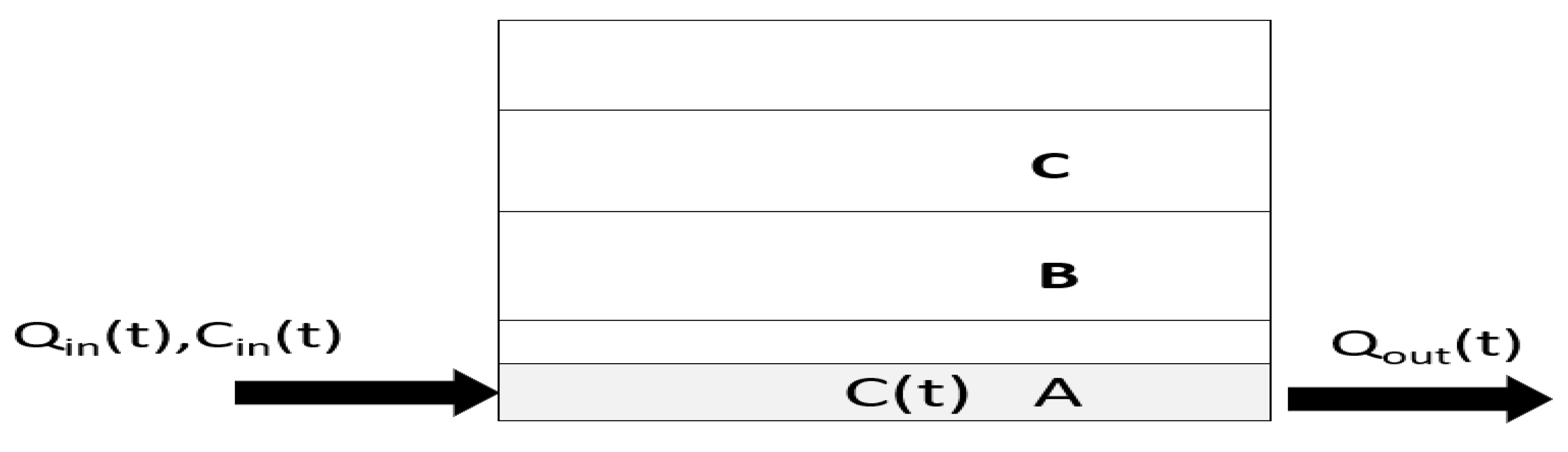
The mixing behaviors inside the tank were modeled in this research using a three-compartment model. Three different compartments make up this model, which approximates the spatial distribution of constituent concentrations. Each of the three compartments was represented as a thoroughly mixed volume element, with the flow and dissolved elements passing directly between them [14]. The tanks were traditional inflow/outflow tanks that fill or drain as needed rather than simultaneously. Assuming that each compartment defines the varied mixing behaviors in a separate tank segment, a basic mass balance equation was used to describe the mixing situation in each compartment. The entry point can come from any compartment, while the outlet is located at the bottom. The chemical compound fluoride (conservative species) was thought to be present in the water. Figure 1 depicts the model schematic where the inlet and initial water level were located at the bottom (Compartment A).
The general formulas describing the change of fluoride/chlorine concentration in each compartment are shown in Equations (1) and (2).
or, equivalently, .
3.1.1. Inflow Conditions
Each compartment’s governing equations were determined by the inlet/outlet configuration and the initial water level in the tank. There were three water input points and three water levels to start with, as shown in Figure 1. When all permutations are taken into account, there are nine tank configurations. The mass balance was used to create the differential equation in each compartment of the nine layouts. In any compartment, concentration fluctuations occurred when different water concentrations were mixed or when the incoming water had a time-dependent inlet concentration. When the compartment was empty and no additional water was being introduced, the concentration remained at zero. Table 1 contains a summary of all cases at the filling stage.
The first column represents the inlet locations, and the first row shows the initial water level. For example, for the first combination, where both the inflow point and the initial water level were in Compartment A, separate differential equations had to be generated for each compartment. In Case 1, the new water arriving was mixed with the old water that was previously present in Compartment A. If the two water concentrations differed, there was a change in concentration in Compartment A. Compartments B and C, on the other hand, contained no concentration because they were both empty in this situation. No additional water entered them during the filling stage of Compartment A.
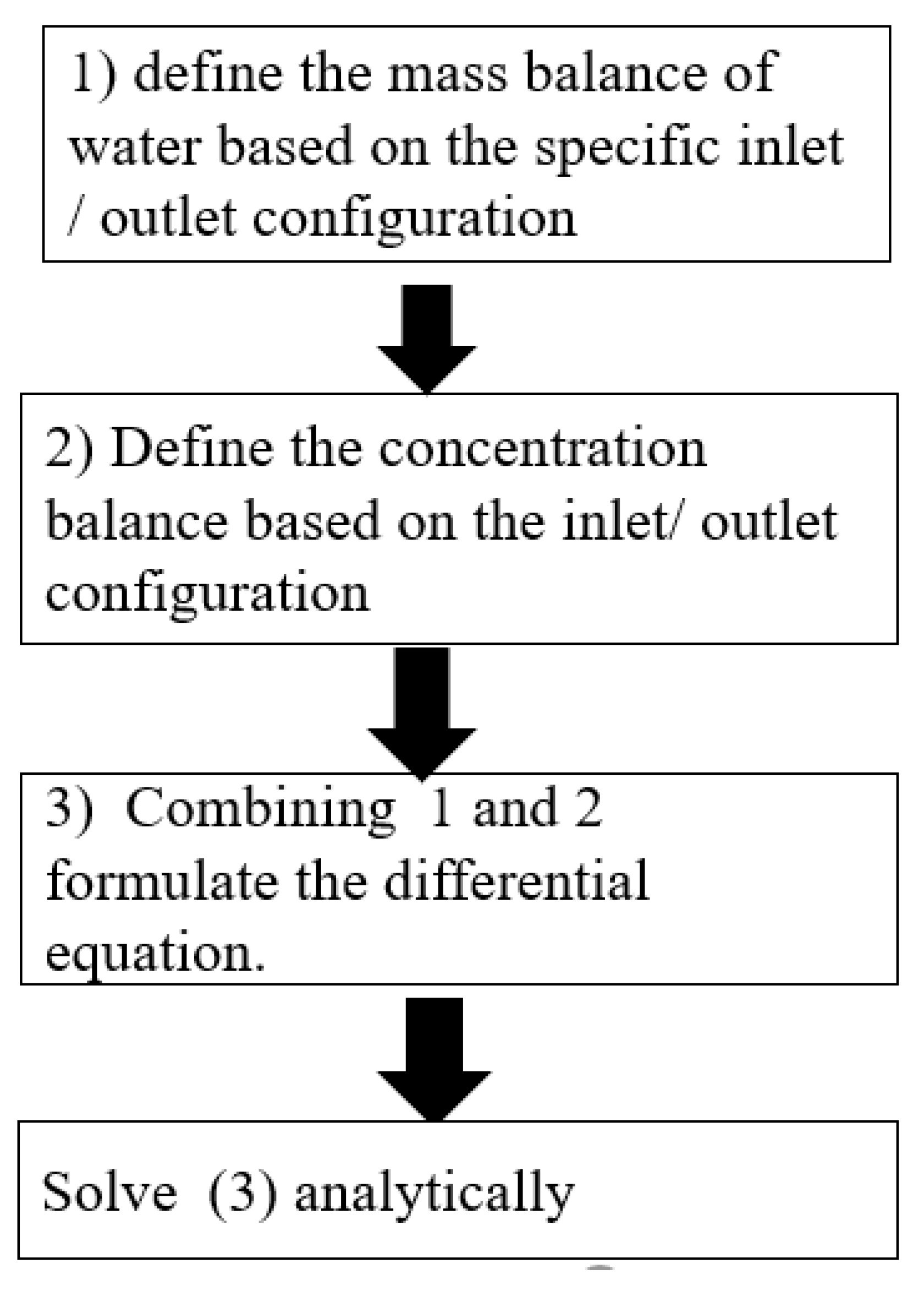
In Case 2, the intake point was positioned in Compartment A, and the initial water level was located in Compartment B. Because Compartment A was full, there was no change in water volume. However, concentrations fluctuated if the intake and starting concentrations in the compartment were not the same. In Case 3, the newly mixed water from Case 2 entered Compartment B straight from Compartment A. In some instances, the resulting differential equation may be symmetric. Cases 1, 7, and 13 were, for example, identical. Even though the inlet locations were different, the mass balance for Compartment A during the filling stage was the same as long as the water level was in Compartment A. When there was no mixing, the concentration remained constant. In Case 8, both the water level and the entry points were initially in Compartment B. This signifies that Compartment A was a dead zone during the filling stage of Compartment B. Because it received no additional water from the outside, its concentration remained constant over this time. Generally, the steps to find an analytical solution for the concentration as a function of time in any compartment are described in Figure 2.
A brief analytical solution formulation for each compartment for all nine-tank arrangements was detailed during the filling cycle. The output point was closed during this period, and there was no outflow (Qout(t) = 0).
Configuration 1: Initial Level of Water and Inlet Point of Compartment A
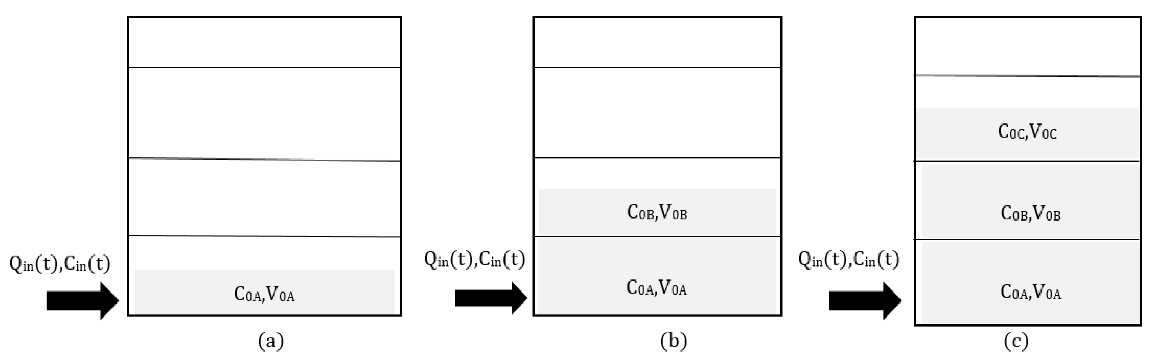
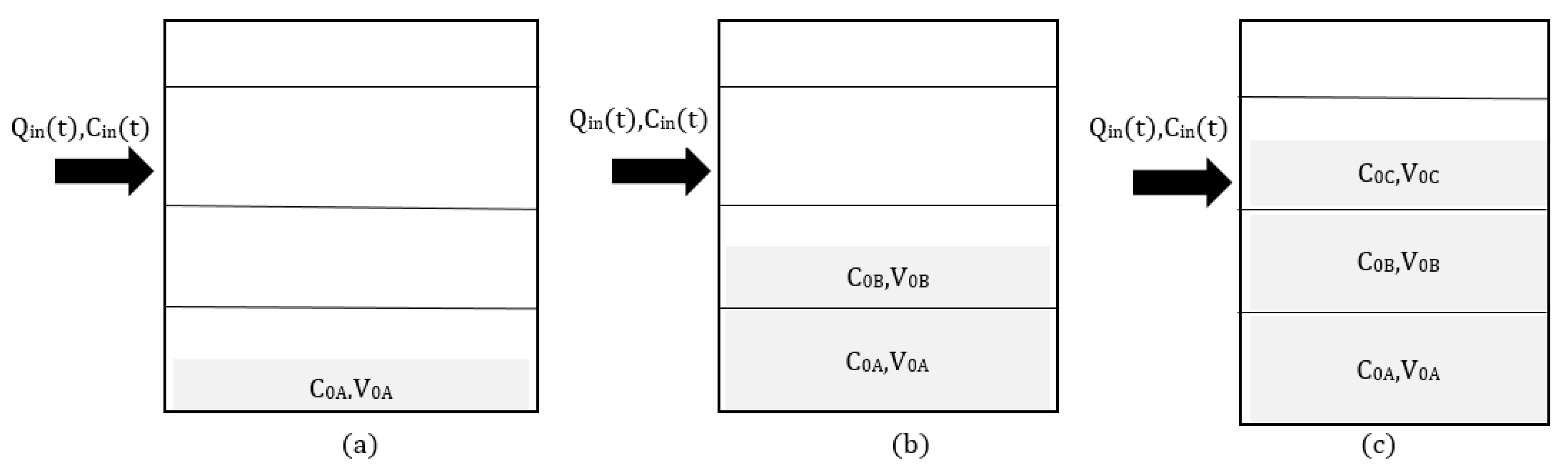
The tank had three compartments, each with fixed volumes of VA, VB, and VC. Calibration was used to determine the capacity of each compartment. Water at a constant flow rate of Qin(t) and a fluoride concentration of Cin(t) was supposed to enter the tank through Compartment A for specific delta t(Δt). Thus, the tank has an initial water volume given as V0A and an initial fluoride content of C0A. Figure 3 shows a graphical representation of the arrangement.
Since there is only filling, .
Combining Equations (5) and (6),
The solution for Equation (7), assuming that , is given as
Compartments B and C have no concentration because they were both empty in this condition, and no more water was entering them during Compartment A’s filling stage.
Configuration 2: Initial Level of Water in Compartment B and Inlet of Compartment A
Initially, Compartment A was full (VA = V0A). The water level in Compartment B had a volume of V0B and a concentration of C0B. Water entered Compartment A at a constant flow rate, Qin(t), and an inlet concentration of Cin(t). Then, it flowed into Compartment B at the same rate as before, with a new fluoride concentration, (8), formed by mixing in Compartment A. Figure 3b shows a graphical representation.
Case 2: Compartment A (Figure 3b).
In this instance, Compartment A was initially full. Water flowed into and out of the compartment at the same rate . The volume remained constant during the filling stage.
Combining Equations (9) and (10),
The analytical solution of Equation (11), assuming that , is given as
Case 3: Compartment B (Figure 3b).
Water entered Compartment B from Compartment A, with the same flow, Qin(t), and a concentration provided by the analytical solution in (12) (. The water level in Compartment B had a volume of V0B and a concentration of C0B. A graphical representation is given in Figure 3b.
Combining Equations (13) and (14),
The analytical solution of Equation (15), assuming that , is
Configuration 3: Initial Level of Water in Compartment C and Inlet of Compartment A
The tank had three compartments, each with fixed volumes of VA, VB, and VC, respectively. The initial water level in Compartment C had a volume of V0C and a concentration of C0C. Water was assumed to enter Compartment A with a constant flow rate, Qin(t), and a fluoride concentration of Cin(t) and flowed into Compartment B and Compartment C with the same flow rate, Qin(t). A graphical representation is shown in Figure 3c.
Case 4: Compartment A (Figure 3c).
This case was the same situation as Case 2; Compartment A was full, and water entered Compartment A. The only difference was that the water level was initially in Compartment C, which did not affect the mixing mechanism in Compartment A. The mass balance equations and solution were the same. The analytical solution was given in (12), .
Case 5: Compartment B (Figure 3c).
Both Compartments A and B were initially full (VA = V0A, VB = V0B). The volume of water in Compartments A and B remained constant during the filling stage of Compartment C. The water level in Compartment C had a volume of V0C and a concentration of C0C. New water flowed into Compartment A with a Cin(t) inlet concentration and Qin(t) flow. It flowed to Compartment B with a new chlorine concentration, given in (12), and to Compartment C with a new chlorine concentration (16), formed by mixing in Compartment B, all at the same flow rate (Qin(t)). Figure 3c depicts a graphical representation of the layout.
Combining Equations (17) and (18)
The analytical solution of Equation (19), assuming that , is
Case 6: Compartment C (Figure 3c).
Initially, the water level was in Compartment C with a volume of V0C and a concentration of C0C. Then, water flowed to Compartment C from Compartment B at a constant flow rate of Qin(t) and the fluoride concentration given in (20). A graphical representation is shown in Figure 3c.
Combining Equations (21) and (22),
The analytical solution for Equation (23), assuming that , is
Configuration 4: Initial Level of Water in Compartment A and Inlet of Compartment B
The tank was divided into three compartments with fixed volumes of VA, VB, and VC. Water was assumed to enter the tank with a constant flow rate of Qin(t) and fluoride concentration of Cin(t) from Compartment B. Thus, the tank had an initial water volume of V0A in Compartment A, with an initial fluoride concentration of C0A. A graphical representation is provided in Figure 4a.
Case 7: Compartment A (Figure 4a).
This case was almost the same situation as Case 1, the only difference being that water with a flow rate of Qin(t) and an inlet concentration of Cin(t) entered Compartment A from Compartment B. The analytical solution for Compartment A in Equation (8) is provided by the following:
Configuration 5: Initial Level of Water in Compartment B and Inlet of Compartment B
The tank was divided into three compartments with fixed volumes of VA, VB, and VC. Initially, the water level was in Compartment B with a volume of V0B and a concentration of C0B. Water entered Compartment B with a constant flow of Qin(t) and a fluoride concentration of Cin(t), as shown in Figure 4b.
Case 8: Compartment A (Figure 4b).
During the filling stage of Compartment B, Compartment A was a dead zone. It did not interact with new water that came from outside through Compartment B. Therefore, the concentration remained constant for Compartment A.
Case 9: Compartment B (Figure 4b).
Initially, the water level in Compartment B had a volume of V0B and a concentration of C0B. Water entered Compartment B with a constant flow rate of Qin(t) and a fluoride concentration of Cin(t), as shown in Figure 4b.
Combining Equations (26) and (27),
The analytical solution of Equation (28), assuming that , is
Configuration 6: Initial Level of Water in Compartment C and Inlet of Compartment B
The tank was divided into three compartments with fixed volumes of VA, VB, and VC. Initially, the water level was in Compartment C with a volume of V0C and a concentration of C0C. Then, water was assumed to enter Compartment B with a constant flow rate of Qin(t) and a fluoride concentration of Cin(t), and left with the same flow, Qin(t).
Case 10: Compartment A (Figure 4c).
There was no mixing since no water entered Compartment A. Therefore, during the filling phase, the concentration remained the same as C0A.
Case 11: Compartment B (Figure 4c).
In this instance, Compartment B was initially full. Water flowed into and out of the compartment at the same rate, . The volume remained constant during the filling stage.
Combining Equations (30) and (31),
The analytical solution of Equation (32), assuming that , is
Case 12: Compartment C (Figure 4c).
Initially, the water level was in Compartment C with a volume of V0C and a concentration of C0C. Water entered Compartment B with at a constant flow rate of Qin(t) and an inlet fluoride concentration of Cin(t). It flowed with the same flow rate, Qin(t), and a concentration of the analytical solution (33) into Compartment C. A graphical representation is given in Figure 4c.
Combining Equations (34) and (35),
The analytical solution for Equation (36) is
Configuration 7: Initial Level of Water in Compartment A and Inlet of Compartment C
The tank was divided into three compartments with fixed volumes of VA, VB, and VC. Water was assumed to enter the tank with a constant flow rate of Qin(t) and a chlorine concentration of Cin(t) from Compartment C. Thus, the tank had an initial water volume of V0A in Compartment A with an initial fluoride concentration of C0A. A graphical representation is given in Figure 5a.
Case 13: Compartment A (Figure 5a).
This case was similar to Cases 1 and 7. Thus, the analytical solution of Compartment A is Equation (8).
Configuration 8: Initial Level of Water in Compartment B and Inlet of Compartment C
The tank was divided into three compartments with fixed volumes of VA, VB, and VC. Water entered the tank with a constant flow rate of Qin(t) and chlorine concentration of Cin(t) from Compartment C. The tank had an initial water volume of V0B in Compartment B with an initial fluoride concentration of C0B. A graphical representation is shown in Figure 5b.
Case 14: Compartment A (Figure 5b).
Since there was no mixing of the concentration in Compartment A, it remained the same as C0A.
Case 15: Compartment B (Figure 5b).
This case was almost the same as Case 9. The only difference was that A water with flow Cin(t) and Qin(t) enters Compartment B from Compartment C. The analytical solution is (29), .
Configuration 9: Initial Level of Water in Compartment C and Inlet of Compartment C
The tank was divided into three compartments with fixed volumes of VA, VB, and VC. Water was assumed to enter the tank with a constant flow rate of Qin(t) and chlorine concentration of Cin(t) from Compartment C. The tank had an initial water volume of V0C in Compartment C with an initial chlorine concentration of C0C. A graphical representation is shown in Figure 5c.
Case 16: Compartment A (Figure 5c).
Since no water flowed into Compartment A, there was no mixing, and the concentration remained constant.
Case 17: Compartment B (Figure 5c).
There was no mixing because no water went into Compartment B during this filling stage. Therefore, the concentration remained constant, at C0B.
Combining Equations (38) and (39),
The analytical solution of Equation (40), assuming that , is
3.1.2. Outflow Conditions
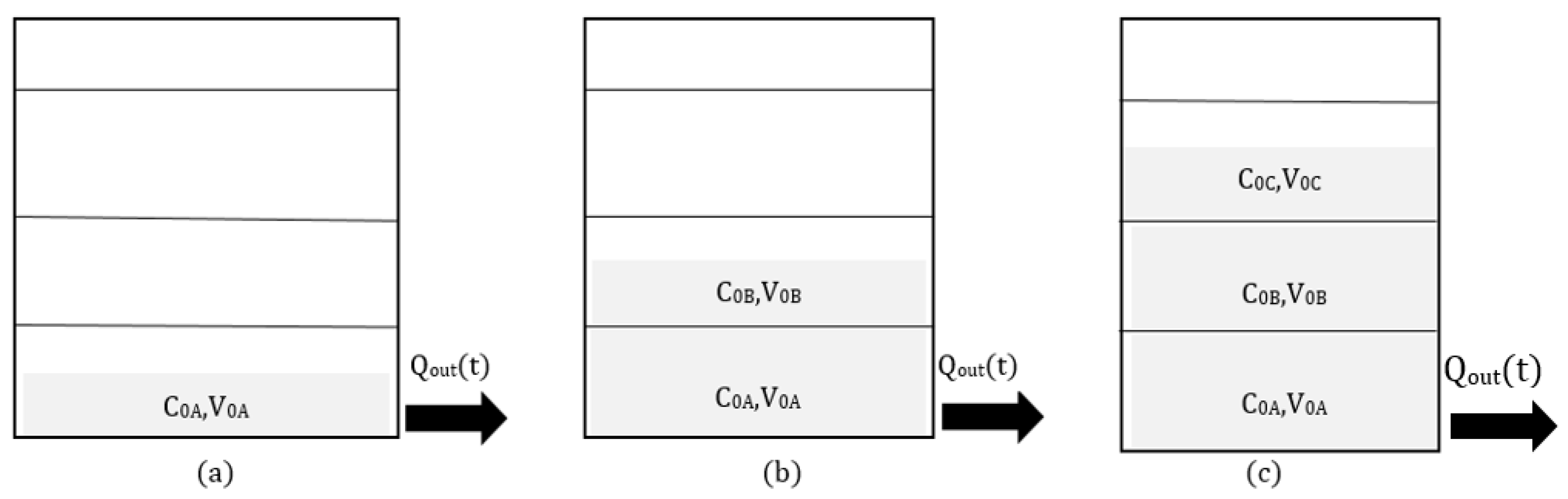
The outlet was located at the bottom of the tank, and the starting water level could come from any of the three compartments. As a result, there were three possible configurations. Unless water with a different concentration flowed from the top compartment, the concentration of any compartment remained constant during the draining process. For example, in Compartment A of the first design depicted in Figure 6a, when the outlet was opened, the water simply flowed without mixing. Therefore, the concentration did not change. Table 3 shows the lists of cases for outflow conditions.
Configuration 1: Outlet Point of Compartment A and Initial Level of the Water in Compartment A
The tank was divided into three compartments with fixed volumes of VA, VB, and VC. Water was assumed to flow out from the tank with a constant flow rate of Qout(t) from Compartment A. Thus, the tank had an initial water volume of V0A in Compartment A with an initial chlorine concentration of C0A. A graphical representation is shown in Figure 6a.
Case 1: Compartment A (Figure 6a).
Because there was no water mixing, the water concentration remained constant at C0A during the draining stage.
Configuration 2: Outlet Point of Compartment A and Initial Level of the Water in Compartment B
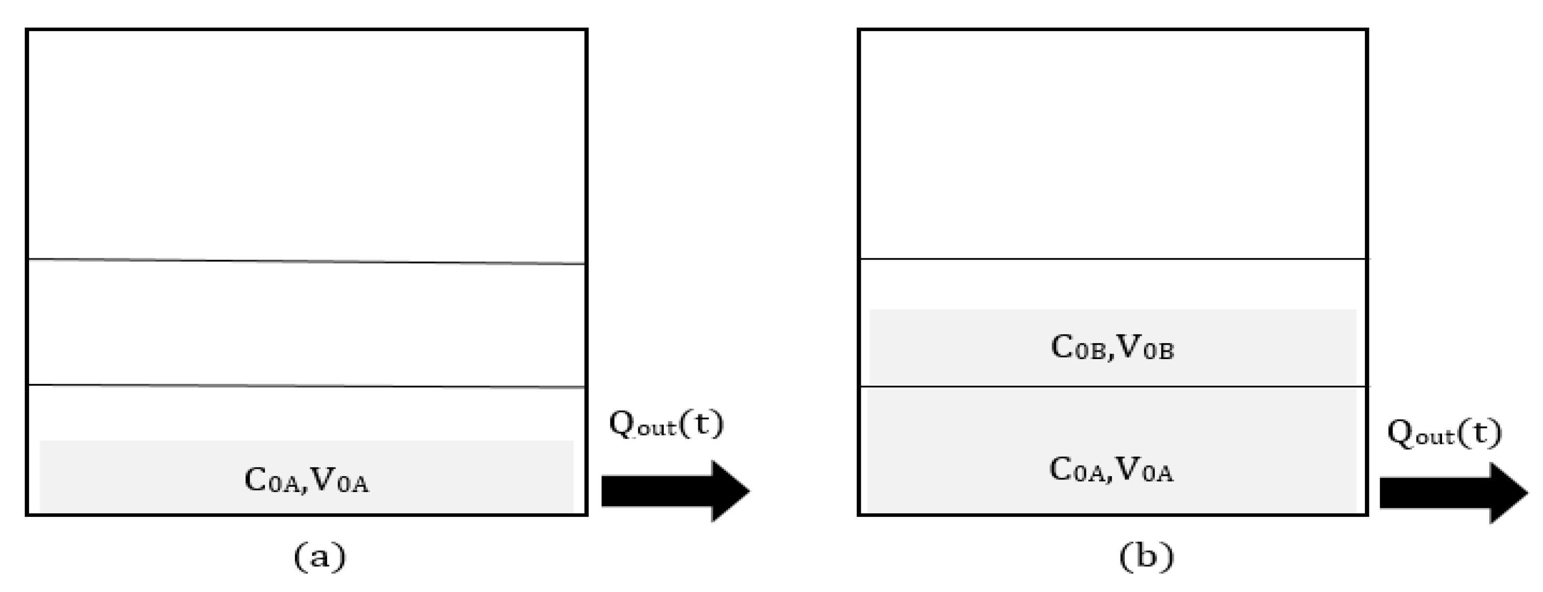
The tank was divided into three compartments with fixed volumes of VA, VB, and VC. Water was assumed to flow out from the tank with a constant flow rate of Qout(t) from Compartment A. The tank had an initial water volume of V0B in Compartment B with an initial chlorine concentration of C0B. Water flowed with the same Qout(t) as in Compartment A. A graphical representation is shown in Figure 6b.
Case 2: Compartment B (Figure 6b).
The water simply flowed without any mixing. The concentration remained constant for Compartment B as .
The tank had an initial water volume of V0B in Compartment B with an initial chlorine concentration of C0B. During Compartment B’s draining stage, the volume of Compartment A remained constant since it was full. Water was assumed to enter Compartment A from Compartment B, with a constant flow rate of Qout(t) with a concentration of C0B, and flow out of the tank with the same flow rate, Qout(t). A graphical representation is shown in Figure 6b.
Combining Equations (41) and (42),
The analytical solution of Equation (43), assuming that , is
Configuration 3: Outlet Point in Compartment A and Initial Level of the Water in Compartment C
The tank was divided into three compartments with fixed volumes of VA, VB, and VC. Water was assumed to leave from the tank with a constant flow rate of Qout(t) from Compartment A. Thus, the tank had an initial water volume of V0C in Compartment C with an initial chlorine concentration of C0C. Water flowed with the same Qout(t) to Compartments A and B. A graphical representation is shown in Figure 6c.
Case 3: Compartment C (Figure 6C).
Water from Compartment C exited without mixing during a specific delta t. As a result, the concentration remained the same as C0C. Water with a concentration of C0c flowed into Compartment B during this period.
Case 4: Compartment B (Figure 6C).
In Compartment C, the tank had an initial water volume of V0C with an initial chlorine concentration of C0B. Because Compartment B was filled, the volume of Compartment B remained constant during the draining step of Compartment C. Water with a concentration of C0C was assumed to enter Compartment B from Compartment C of the tank at a constant flow rate of Qout(t).
Combining Equations (45) and (46)
The analytical solution of Equation (47), assuming that , is
Case 5: Compartment A (Figure 6c).
The tank had an initial water volume of V0c in Compartment C with an initial chlorine concentration of C0C. Water was assumed to enter Compartment B from Compartment C of the tank with a constant flow rate of Qout(t) and concentration of C0c at this specific delta T. Water with the same flow but a concentration of ( entered Compartment A. Because Compartment A was filled, the volume of Compartment B remained constant during the draining step of Compartment C. A graphical representation is shown in Figure 5c:
Combining Equations (49) and (50),
The analytical solution of Equation (51), assuming that , is
3.2. Non-Conservative Material
The mixing behaviors inside the tank were depicted using a two-compartment model. The tanks were classic inflow/outflow tanks, which are filled or drained according to need rather than simultaneously. The entrance can come from any compartment, and the outlet is at the bottom. It was assumed that the material was non-conservative and had a first-order decay constant of k. The general formulas, which describe the change in the concentration of chlorine are as follows:
or, equivalently,
Inflow Conditions
Using the same analysis as before, the entrance point and the initial water level could be in any of the two compartments for the filling stage. Accordingly, there were four configurations. Table 5 lists all the cases for the inflow stages.
Configuration 1: Initial Level of Water in Compartment A and the Inlet of Compartment A
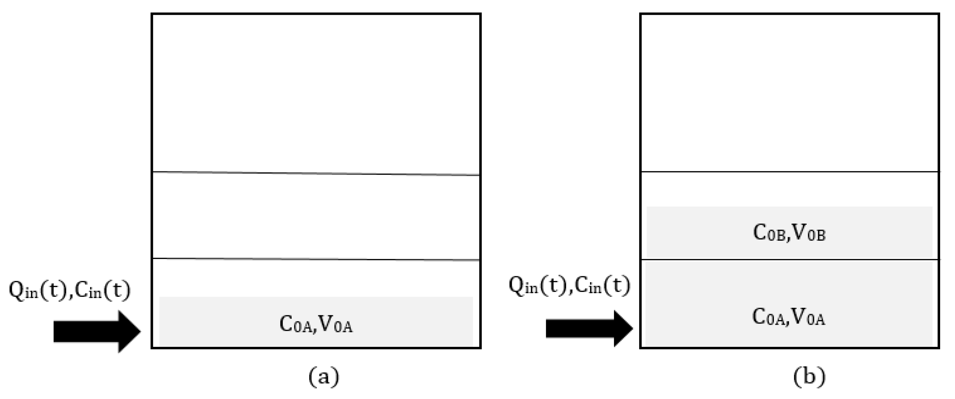
The tank was divided into three compartments with fixed volumes of VA and VB. Water was assumed to enter the tank with a constant flow rate of Qin(t) and chlorine concentration of Cin(t). Thus, the tank had an initial water volume of V0A in Compartment A with an initial chlorine concentration of C0A with a decay constant K. Figure 7a shows a graphical representation.
Combining Equations (57) and (58),
The analytical solution of Equation (59), assuming that , is
Configuration 2: Initial Level of Water in Compartment B, and the Inlet of Compartment A
The tank was divided into two compartments with fixed volumes of VA and VB. Water was assumed to enter the tank with a constant flow rate of Qin(t) and chlorine concentration of Cin(t). The tank had an initial water volume of V0B in Compartment B with an initial chlorine concentration of C0B with a decay constant K. Compartment A was full. Figure 7b shows a graphical representation.
Combining Equations (61) and (62),
The analytical solution of Equation (63), assuming that , is
Case 3: Compartment B (Figure 7b).
Initially, the water level in Compartment B had a volume of V0B and a concentration of C0B. Water was assumed to enter Compartment A with a constant flow rate of Qin(t) and chlorine concentration of Cin(t), which has a decay constant K and leaves with the same flow, Qin(t), and a concentration of the analytical solution of Equation (48) into Compartment B. A graphical representation is provided in Figure 7b.
Combining Equations (65) and (66),
The analytical solution of Equation (67), assuming that , is
Configuration 3: Initial Level of Water in Compartment A and the Inlet of Compartment B
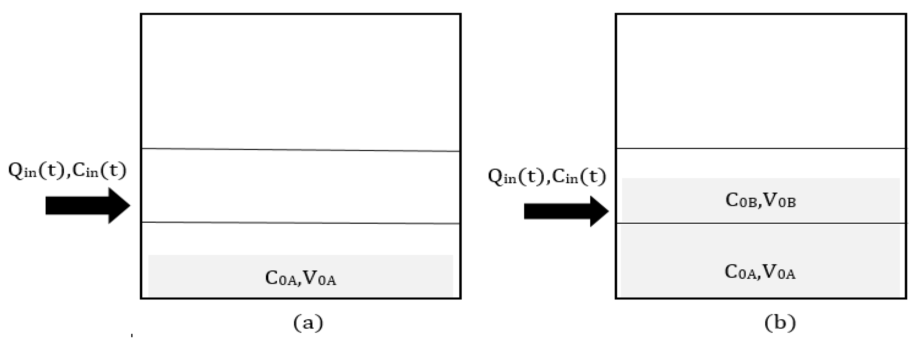
The tank was divided into two compartments with fixed volumes of VA and VB. Water was assumed to enter the tank with a constant flow rate of Qin(t) and chlorine concentration of Cin(t) from Compartment B. The tank had an initial water volume of V0A in Compartment A with an initial chlorine concentration of C0A with a decay constant K. Figure 8a shows a graphical representation.
Case 4: Compartment A (Figure 8a).
This was almost the same as Case 1, with the only difference being the water inlet location. The analytical solution is given in Equation (60).
Configuration 4: Initial Level of Water in Compartment B and the Inlet of Compartment B
The tank was divided into two compartments with fixed volumes of VA and VB. Water was assumed to enter the tank with a constant flow rate of Qin(t) and chlorine concentration of Cin(t) from Compartment B. Thus, the tank had an initial water volume of V0B in Compartment B with an initial chlorine concentration of C0B with a decay constant K. A graphical representation is shown in Figure 8b.
Case 5: Compartment A (Figure 8b).
The water in the compartment is not interacting with any new water that comes from outside during the filling stage.
Combining Equations (69) and (70),
The solution of Equation (71) is .
Case 6: Compartment B (Figure 8b).
Initially, the water level was in Compartment B with a volume of V0B and concentration of C0B with a decay constant K. water was assumed to enter Compartment B with a constant flow rate of Qin(t) and chlorine concentration of Cin(t) as shown in Figure 8b:
Combining Equations (72) and (73),
The analytical solution of Equation (74), assuming that , is
Table 6 refers the summary of the analytical solutions.
3.3. Outflow Condition
The draining procedure was also subjected to the same scrutiny as the conservative procedure. Suppose there is no mixing in the compartment when the outlet is opened; unlike the conservative ones, the concentration changes due to the decay constant. There are two configurations that can be achieved by changing the initial water level. Table 7 shows the list of the cases.
3.3.1. Configuration 1: Initial Level of Water in Compartment A and the Outlet of Compartment A
The tank was divided into two compartments with fixed volumes of VA and VB. Water was assumed to leave from the tank with a constant flow rate of Qout(t) from Compartment A. The tank had an initial water volume of V0A in Compartment A with an initial chlorine concentration of C0B and a decay constant K. Water flows with the same Qout(t) as Compartment A. A graphical representation is shown in Figure 9a.
Combining Equations (76) and (77),
The solution of Equation (78) is
3.3.2. Configuration 2: Initial Level of Water in Compartment B and the Outlet of Compartment A
The tank was divided into two compartments with fixed volumes of VA and VB. Water was assumed to leave from the tank at a constant flow rate of Qout(t) from Compartment A. The tank had an initial water volume of V0B in Compartment B with an initial chlorine concentration of C0B, and a decay constant K. Water flows with the same Qout(t) to Compartment A. A graphical representation is shown in Figure 9b.
Combining Equations (80) and (81),
The solution of Equation (82) is
Case 2: Compartment A (Figure 9b).
Water was assumed to leave from the tank with a constant flow rate of Qout(t) from Compartment A. The tank had an initial water volume of V0B in Compartment B with an initial chlorine concentration of C0B, and a decay constant K. Water flows with the same Qout(t) and a concentration of to Compartment A. During this time, Compartment A was full. Figure 6b gives a graphical representation.
Combining Equations (84) and (85),
The solution of Equation (86), assuming that , is
Table 8 summarize the analytical solutions.
4. Example Application
For both the filling and draining stages, full analytical solutions were developed, taking into account all the combinations and arrangements for both conservative and non-conservative materials. A simulation can be run to calculate the volume and concentration at any time in a specified compartment by providing all of the necessary input variables. A user enters the following as inputs:
- −
- The fixed volumes of Compartments A, B, C; a calibration was used to choose the volume of each compartment.
- −
- The delta t and total simulation time T.
- −
- The inlet points.
- −
- The initial levels and volumes of water and the initial concentrations.
- −
- The inflow Qin(t) with its Cin(t) and outflow Qout(t) for different delta t (during total time T).
Using the appropriate equation, concentrations were calculated at any time for each compartment. In addition, the results were validated by comparing them with numerical results.
The following are assumed to be true for the flow.
- −
- Constant for specific delta t.
- −
- It can be either filling (Qout = 0) or draining (Qin = 0) at any time.
- −
- It was given for the total simulation time T.
When it was filling (Qin > 0), there was a Cin(t) (inlet concentration).
A sample of theoretical data and field data from [11] were taken to test the model for both conservative and non-conservative constituents.
4.1. Conservative Material
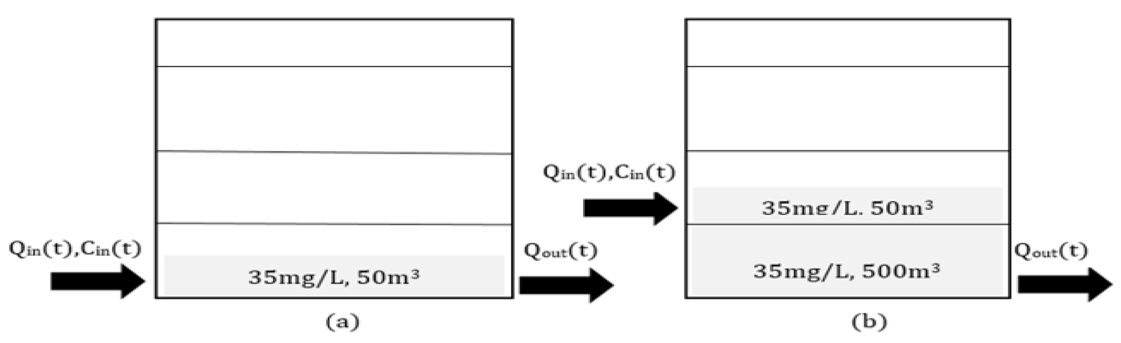
A tank was divided into three compartments and had volumes of 500 m3, 400 m3, and 600 m3, starting from the bottom. The simulation was carried out for a total of 10 h, with delta t (Δt) being 1 h. The flow at each hour is given in Table 9.
Two arrangements (initial levels of water concentrations) are presented in Figure 10.
Result and Discussion
Using the appropriate equations, the volumes and concentrations were calculated at each time step. The volume and concentration graphs are presented as follows.
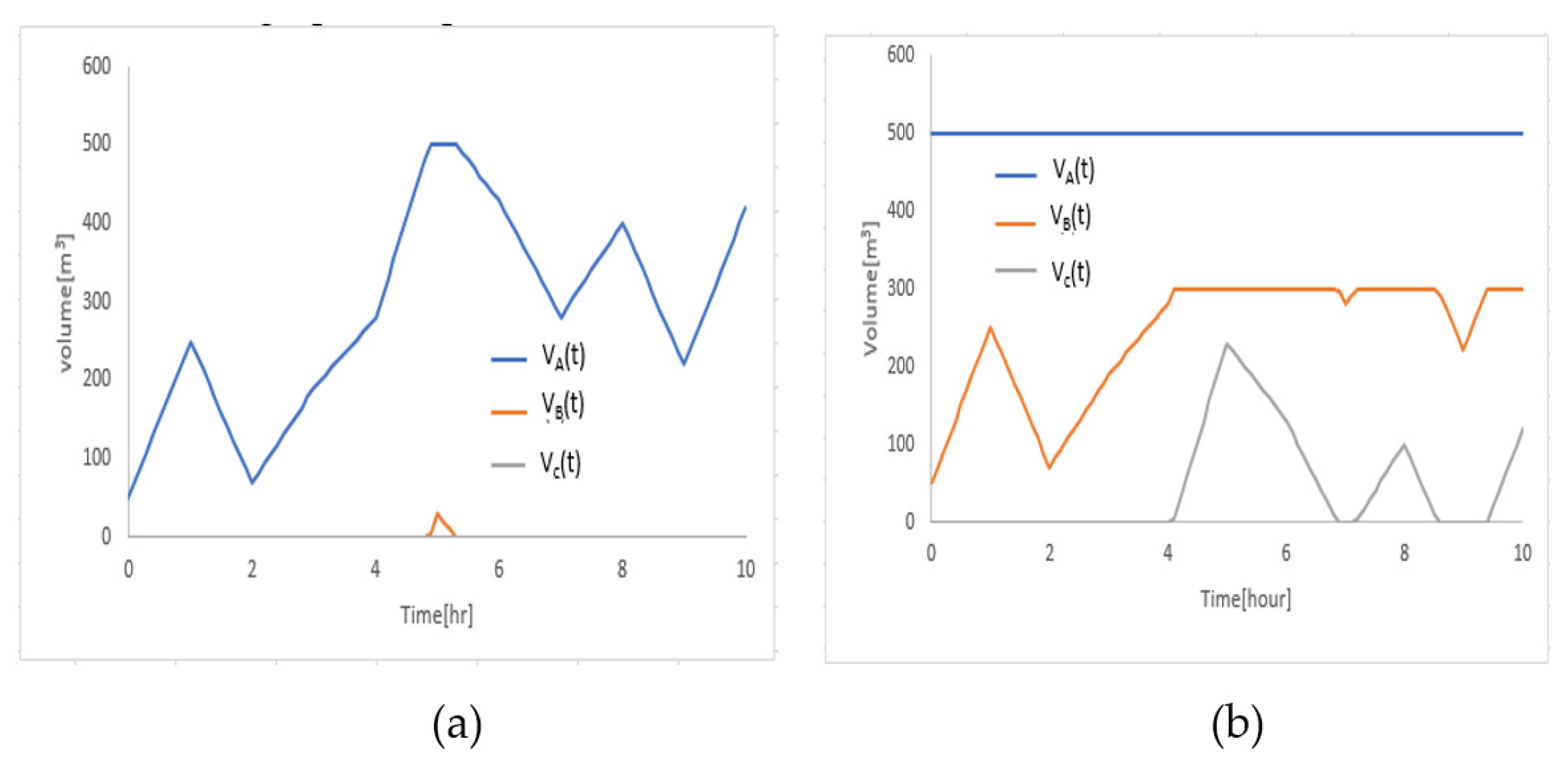
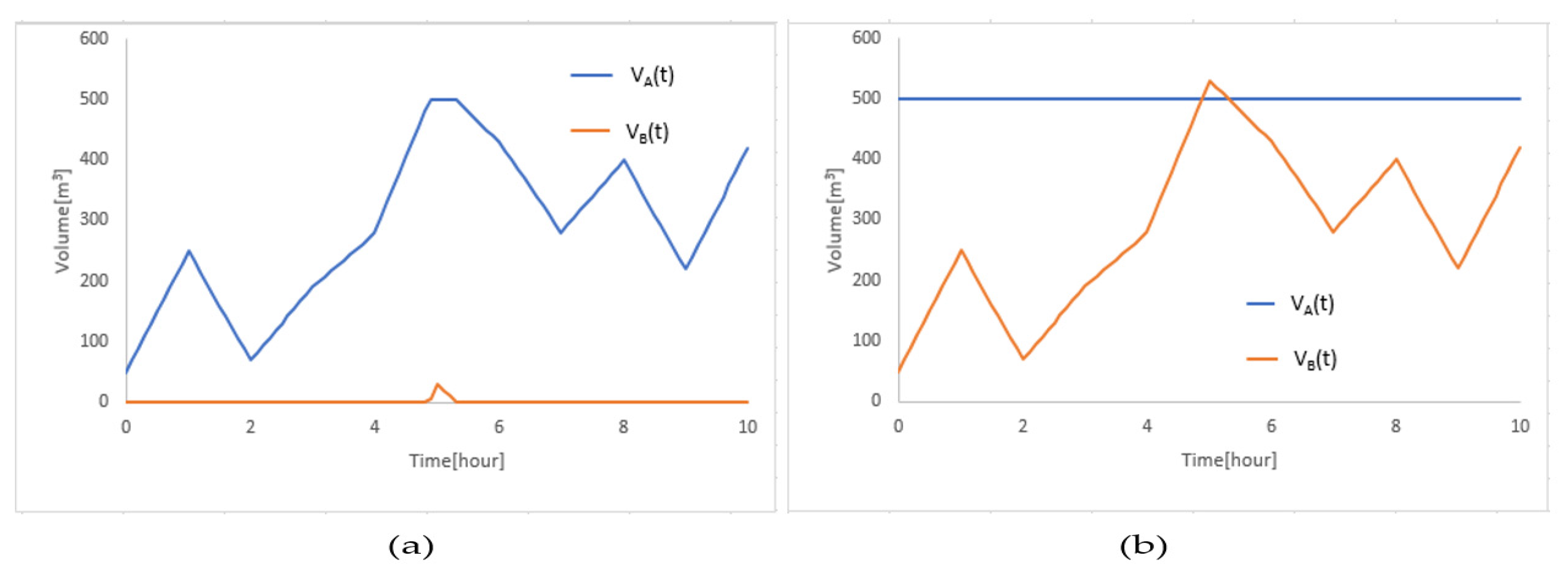
Figure 11 shows the volume of each compartment as a function of time. In (a), at first, Compartment A contained 50 m3 of water. It rose when there was inflow and fell when there was outflow, according to the flow tables. Water flowed into Compartment B when it exceeded its capacity volume of 500 m3, increasing the volume of Compartment B. The water level did not reach Compartment C in this flow example. As a result, the volume of Compartment C was nil. (b) Initially, Compartment A contained 500 m3 of water (maximum capacity), while Compartment B had 50 m3 of water. The volume in Compartment A remained constant according to the flow tables, while the volume in Compartment B increased when there was inflow and reduced when there was outflow. Water flowed into Compartment C when it exceeded its capacity volume of 300 m3, increasing the volume of Compartment C.
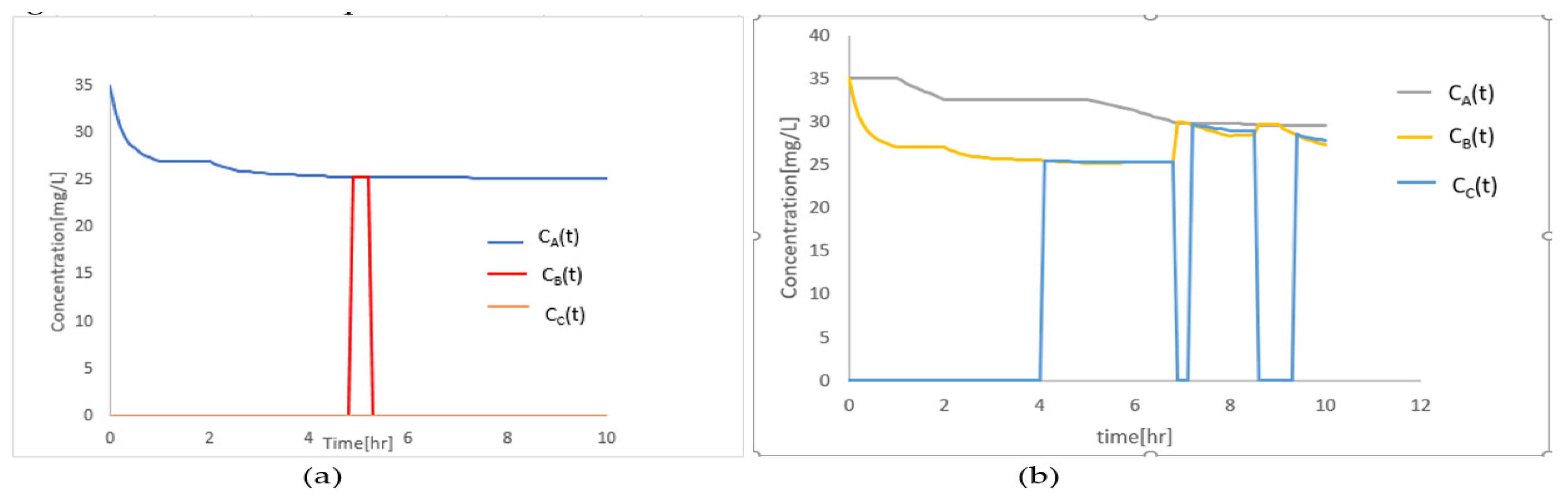
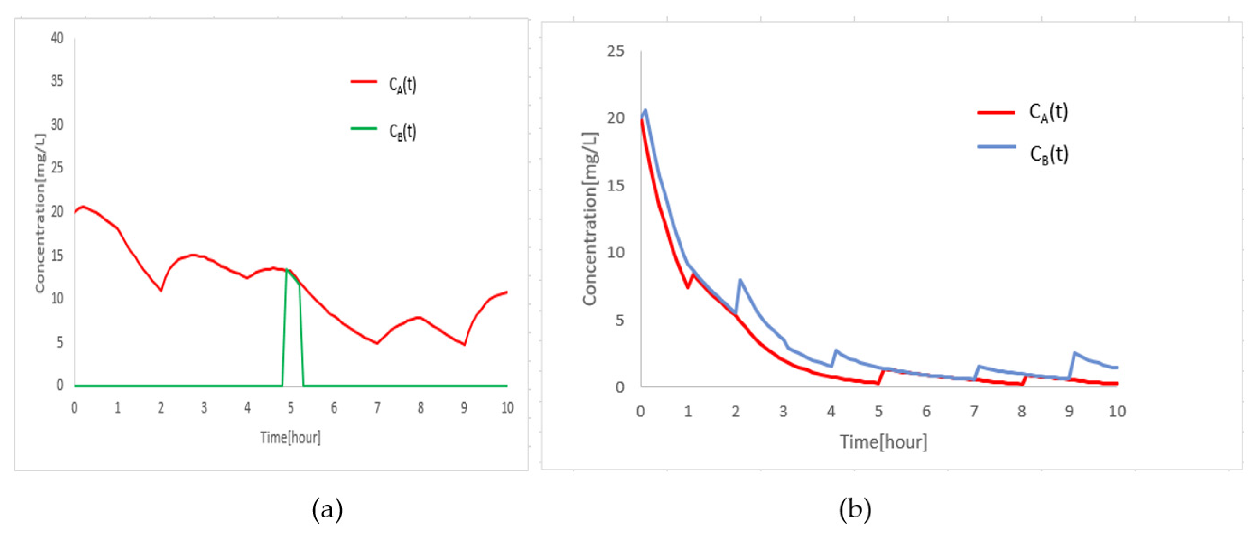
Figure 12 shows the fluoride concentration as a function of time. Because the material was conservative, the concentration inside each compartment rose or fell with time to approach the inlet concentration in both arrangements. Compartment A had a 35 mg/L concentration in (a). It lowered over time since it was more than the inlet concentration (25 mg/L). Because there was no water in Compartments B and C, the concentrations were zero. When water entered Compartment B, the concentration instantly rose and gradually approached the input concentration until it reached zero, when the water level returned to Compartment A. The water level did not reach Compartment C in these specific situations. As a result, the concentration always stayed zero. For the second configuration (b), Compartments A and B had 35 mg/L concentrations at first. Because the entrance came from Compartment B, in the first hour of filling, mixing occurred only in Compartment B. As a result, although Compartment B’s concentration decreased to approach the inflow concentration, Compartment A’s concentration remained unchanged. Whenever Compartment B was draining, water with a certain concentration flowed into Compartment A. The concentration in Compartment A lowered to maintain equilibrium.
Since the water level reached Compartment C in the fourth hour, the concentration of the water increased rapidly.
4.2. Non-Conservative Material
A tank was divided into two compartments and had volumes of 500 m3 and 650 m3, starting from the bottom. The simulation was carried out for a total of 10 h, with delta t (Δt) at 1 h. The flow rate at each hour is provided in Table 9. The decay constant K was taken as 0.5. Two arrangements (initial levels of water and initial concentrations) are presented in Figure 13.
Results and Discussion
Using the appropriate equations, the volume and concentrations were calculated at each time step. The volume and concentration graphs are presented as follows.
Figure 14 shows the volume of each compartment as a function of time. (a) At first, Compartment A contained 50 m3 of water. It rose when there was inflow and fell when there was outflow, according to the flow tables. Water flowed into Compartment B when it exceeded its capacity volume of 500 m3, increasing the volume of Compartment B. (b) At first, Compartment A contained 500 m3 of space (their maximum capacity). The volume of water in Compartment B was 50 m3. The volume in Compartment A was constant, according to the flow tables. Due to the unique flow arrangement, only Compartment B experienced a change in volume.
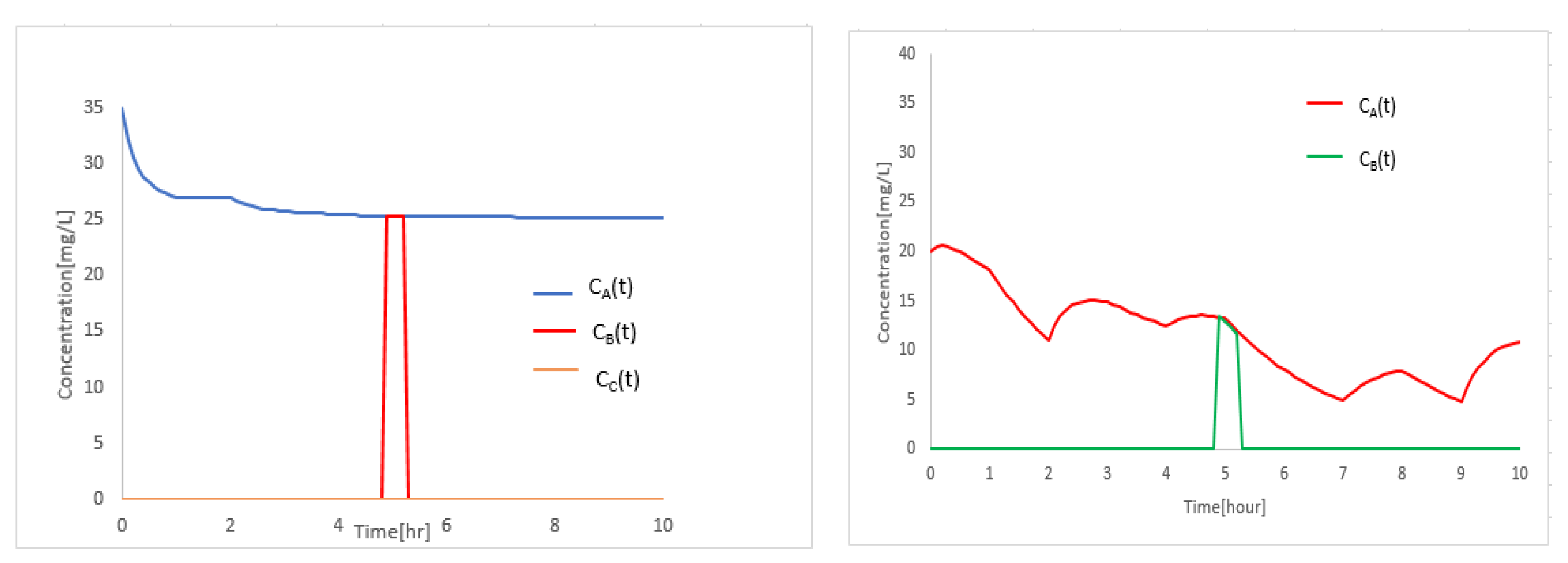
Figure 15 illustrates the graph of concentration as a function of time. (a) Unlike the conservative material, the concentration changed not only because of mixing, but also as a result of the effect of decay constant K. Initially, the concentration in Compartment A was 20 mg/L. The concentration inside the tank began to rise, approaching the higher inlet concentration of 25mg/L. However, because of the decay constant K, it instantly began to decline. If new water entered the tank with an inlet concentration that was higher than the concentration inside the tank, the concentration rose to maintain equilibrium. This may be seen in the graphs for the second, fourth, seventh, and ninth hours. (b) Initially, the concentrations in Compartments A and B were the same at 20 mg/L. Due to the decaying constant and the full initial volume, it began to decline instantly in Compartment A. In Compartment B, the concentration rose at first due to the higher input concentration but then fell due to the decaying constant. If new water entered the tank with an inlet concentration that was higher than the concentration inside the tank, the concentration rose to maintain equilibrium. This can be seen in the graph for Compartment B in the second, fourth, seventh, and ninth hours, and Compartment A in the first, fifth, and eighth hours. The decay constant prevented a full equilibrium like that of the conservative material. For all non-conservative materials, if the decay constant value k approached zero, the graph resembles that of a conservative material.
The above answers were discovered using analytical methods, and the results were validated by comparing them to numerical finite difference methods. Once the differential equations were developed, rather than solving them analytically, a numerical finite difference method was applied to generate the concentration at each time step using the previous values for both arrangements given in Figure 10a and Figure 13a. Figure 16 shows the numerical solution.
The numerical and analytical results for each compartment are nearly identical. Furthermore, if they are plotted on the same graph, they overlap. This is because analytical solutions are the exact solutions derived from a differential equation with a constant coefficient and are separable rather than approximation solutions.
4.3. Field Example
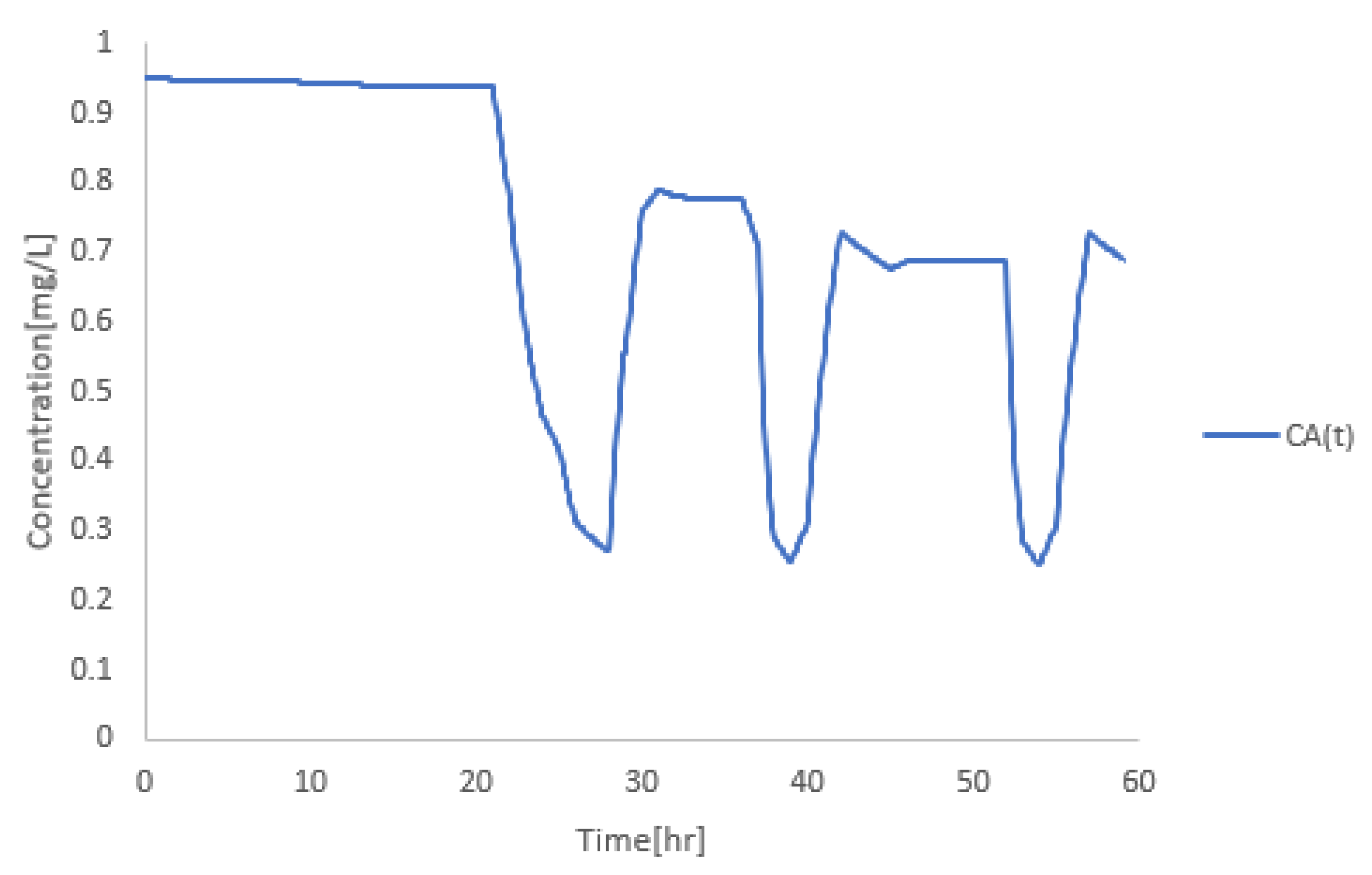
To test the model, empirical data was taken from the previous study conducted by [11]. The obtained field data was a part of a large-scale field investigation conducted in [4]. The concentrations of the tracers were measured at the inlet and outlet of the tank. The research was carried out in the Cherry Hill Brushy Plains service area, which is virtually exclusively residential, with single-family homes and apartment/condominium units. The Cherry Hill pump station pumps water from the Saltonstall system into the service area. The Brushy Plains tank provides storage inside the Cherry Hill Brushy Plains service region. The pumps’ operation is dictated by the water level in the Brushy Plains tank, which has a volume of 3790 m3. The pumps are configured to activate when the water height in the tank lowers to 17.0 m, and to turn off when the elevation reaches 19.7 m in typical conditions. The fluoride feed was shut off at the Saltonstall plant, which supplies the system to record the fluoride residual.
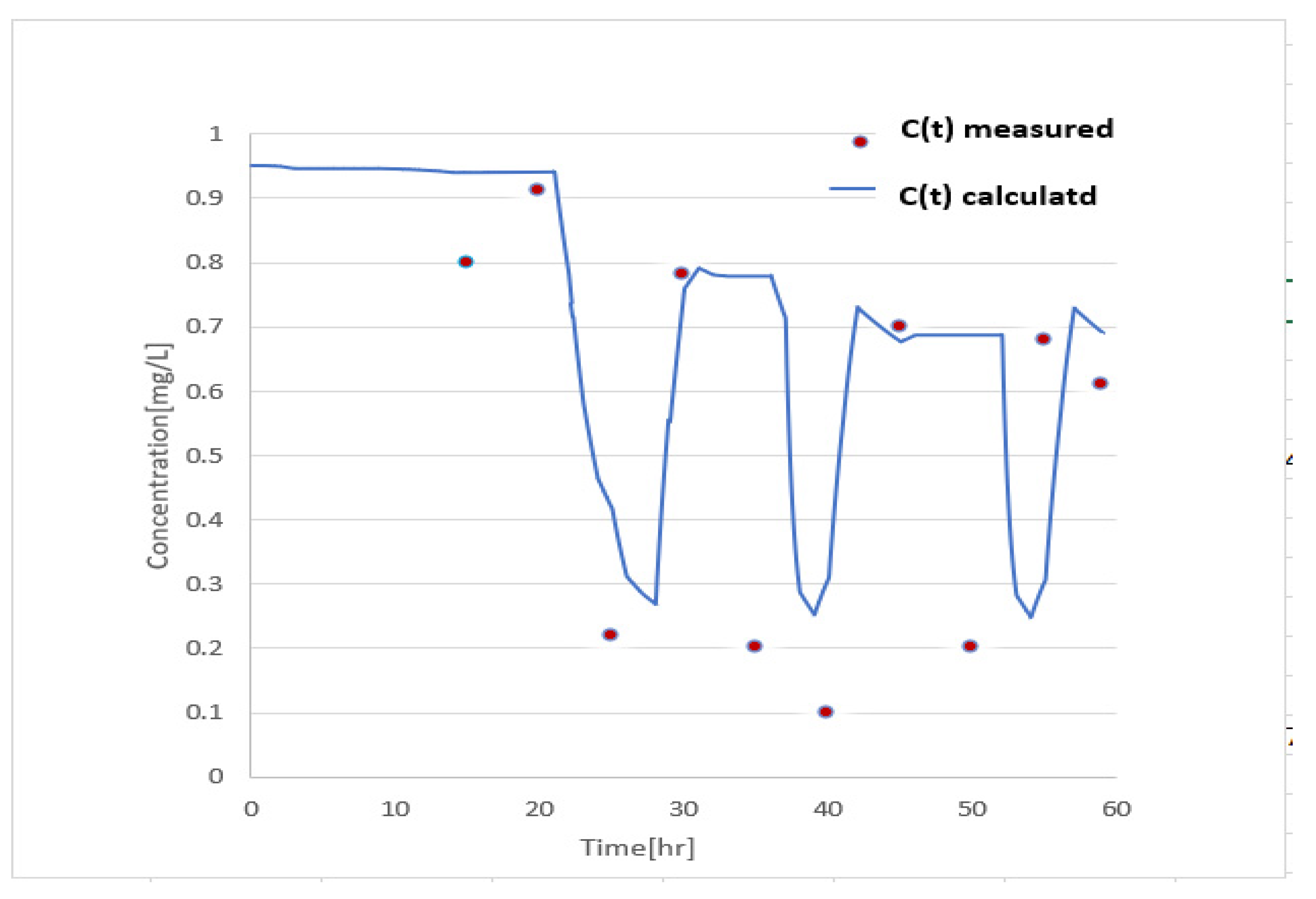
The study in [11] used a three-compartment model, with the bottom and top compartments presumed to be dead zones. Only in the middle did the volume shift. This was relaxed on this model by allowing every compartment to change its volume according to the flow. After regressing the calculated outcomes against the observed data from the effluent data and calculating the relevant R-squares, the 30–40–30 arrangement was discovered to be the best fit [11]. 3030 m3 of water was initially present in the tank. The fluoride content (conservative species) was 0.95 mg/L at the start. The flows were time dependent. To fit into the model developed, an average was taken. The input variables were applied to the model developed. Figure 17 shows the calculated fluoride residuals with respect to time. A comparison was made with the field results found in the same study in Figure 18. The red dots in Figure 18 present some of the results found from the field measurements.
The good fit of the model-generated data to the field-measured data for fluoride supports the use of the compartment models to approximate tank mixing hydrodynamics. More field data and measurements are needed for more confirmation.
5. Conclusions
For anticipating system reactions and pollutant migration and fate, mathematical modeling is a useful tool. However, the majority of published model results are based on the assumption of complete and immediate material mixing. The physical processes that describe the complicated internal mixing and flow interchange characteristics that occur within distribution storage facilities have largely been overlooked.
This study presented a compartment model to characterize mixing behavior inside the tanks. A governing equation was formulated that was dependent on the inlet point and the level of water. The differential equations were solved through the analytical method, and their validity was compared with the results of the numerical solutions. The flows were traditional inflow/outflow methods where only one of them happens for specific delta t. Four example applications with two different arrangements were reviewed to apply the solutions. The solutions fit with the physical assumptions that the concentration inside the tanks either decreases or increases to approach the concentration that comes; it increased when the concentration inside the tank was less than the concentration that was coming and vice versa. Concentration changes happened either because of mixing water with two different concentrations or if there was a time-dependent inlet concentration. The analytical solutions were compared to numerical results and no differences were found; this is because the differential equation is solvable, and an exact solution can be found without approximation. This model can be incorporated into the optimization problem. Field data was applied to the model and there was a good fit between the results of the model and the field measurements.
The substances for the non-conservative material assumed in this paper were used in only two compartments, which identifies the potential future direction of this work. Further study can be done on a decaying material by adding compartment numbers. The model developed here can be incorporated into multi-objective optimization problems in water distribution system-related problems, such as the least costly design, operation, water age, and others.
Author Contributions
Conceptualization, B.A.; data curation, B.A.; formal analysis, B.A.; funding acquisition, A.O.; methodology, A.O.; project administration, A.O.; supervision, A.O.; validation, A.O.; visualization, B.A.; writing—original draft, B.A.; writing—review and editing, B.A. and A.O. All authors have read and agreed to the published version of the manuscript.
Funding
This research was funded by the ISRAEL SCIENCE FOUNDATION (grant No. 555/18).
Institutional Review Board Statement
Not applicable.
Informed Consent Statement
Informed consent was obtained from all subjects involved in the study.
Data Availability Statement
The data presented in this study are available upon request from the corresponding author.
Conflicts of Interest
The authors declare no conflict of interest.
References
- Rossman, L.A.; Uber, J.G.; Grayman, W.M. Modeling disinfectant residuals in drinking-water storage tanks. J. Environ. Eng. 1995, 121, 752–755. [Google Scholar] [CrossRef]
- Gualtieri, C. Analysis of Flow and Concentration Fields in a Baffled Circular Storage Tank. Available online: https://www.researchgate.net/publication/236964353 (accessed on 10 July 2021).
- Mahmood, F.; Pimblett, J.G.; Grace, N.O.; Grayman, W.M. Evaluation of water mixing characteristics in distribution system storage tanks. J. Am. Water Work. Assoc. 2005, 97, 74–88. [Google Scholar] [CrossRef]
- Grayman, W.M.; Clark, R.M. Using computer models to determine the effect of storage on water quality. J. Am. Water Work. Assoc. 1993, 85, 67–77. [Google Scholar] [CrossRef]
- Grayman, W.M.; Rossman, L.A.; Deininger, R.A.; Smith, C.D.; Arnold, C.N.; Smith, J.F. Mixing and aging of water. J. Am. Water Work. Assoc. 2004, 96, 70–80. [Google Scholar] [CrossRef]
- Sathasivan, A.; Fisher, I.; Kastl, G. Application of the microbial decay factor to maintain chloramine in large tanks. J. Am. Water Work. Assoc. 2010, 102, 94–103. [Google Scholar] [CrossRef]
- Ike, N.R.; Wolfe, R.L.; Means, E.G. Nitrifying bacteria in a chloraminated drinking water system. Water Sci. Technol. 1988, 20, 441–444. [Google Scholar] [CrossRef]
- Martel, K.D.; Kirmeyer, G.J.; Murphy, B.M.; Noran, P.F. Preventing water quality deterioration in finished water storage facilities. J. Am. Water Work. Assoc. 2002, 94, 139–148. [Google Scholar] [CrossRef]
- Burlingame, G.A.; Dann, R.M.; Brock, G.L. A case study of geosmin in Philadelphia’s water. J. Am. Water Work. Assoc. 1986, 78, 56–61. [Google Scholar] [CrossRef]
- Grayman, W.M.; Deininger, R.A.; Green, A.; Boulos, P.F.; Bowcock, R.W.; Godwin, C.C. Water quality and mixing models for tanks and reservoirs. J. Am. Water Work. Assoc. 1996, 88, 60–73. [Google Scholar] [CrossRef]
- Clark, R.M.; Abdesaken, F.; Boulos, P.F.; Mau, R.E. Mixing in distribiution system storage tanks: Its effect on water quality. Water Supply 1996, 122, 814–821. [Google Scholar]
- Bangalore, P.N. Scholars’ Mine. Mixing Dynamics in Municipal Water Storage Tanks. Master’s Thesis, Missouri University of Science and Technology, Rolla, MO, USA, September 2016. [Google Scholar] [CrossRef]
- Johnson, D.W.; Johnson, R.T.; Ortiz, A.E.; Stanne, M. Numerical Methods for modeling water quality in distribution systems: A comparison. Phys. Ther. 2001, 81, 1339–1350. [Google Scholar] [CrossRef]
- Boulos, P.F.; Altman, T.; Jarrige, P.A.; Collevati, F. An event-driven method for modelling contaminant propagation in water networks. Appl. Math. Model. 1994, 18, 84–92. [Google Scholar] [CrossRef]
- Mau, R.E.; Boulos, P.F.; Clark, R.M.; Grayman, W.M.; Tekippe, R.J.; Trussell, R.R. Explicit Mathematical Models of Distribution Storage Water Quality. J. Hydraul. Eng. 1995, 121, 699–709. [Google Scholar] [CrossRef]
- Boulos, P.F.; Mau, R.E.; Clark, R.M. Analytical equations of storage reservoir water quality. Civ. Eng. Syst. 1998, 15, 171–186. [Google Scholar] [CrossRef]
- Rossman, L.A. EPANET 2 Users Manual EPA/600/R-00/57; United States Environmental Protection Agency: Washington, DC, USA, 2000.
- Zeidan, M.; Li, P.; Ostfeld, A. DMA Segmentation and multiobjective optimization for trading off water age, excess pressure, and pump operational cost in water distribution systems. J. Water Resour. Plan. Manag. 2021, 147, 04021006. [Google Scholar] [CrossRef]
Figure 1.
A tank with three compartments (A, B, C).

Figure 2.
Model development steps for each compartment.

Figure 3.
A three-compartment model with an inlet point in Compartment A. (a) Initial water level in Compartment A, (b) initial water level in Compartment B, and (c) initial water level in Compartment C.
Figure 3.
A three-compartment model with an inlet point in Compartment A. (a) Initial water level in Compartment A, (b) initial water level in Compartment B, and (c) initial water level in Compartment C.

Figure 4.
A three-compartment model with an inlet point in Compartment B. (a) Initial water level in Compartment A, (b) initial water level in Compartment B, and (c) initial water level in Compartment C.
Figure 4.
A three-compartment model with an inlet point in Compartment B. (a) Initial water level in Compartment A, (b) initial water level in Compartment B, and (c) initial water level in Compartment C.

Figure 5.
A three-compartment model with an inlet point in Compartment C. (a) Initial water level in Compartment A, (b) initial water level in Compartment B, and (c) initial water level in Compartment C.
Figure 5.
A three-compartment model with an inlet point in Compartment C. (a) Initial water level in Compartment A, (b) initial water level in Compartment B, and (c) initial water level in Compartment C.

Figure 6.
A three-compartment model configuration with outlet point in Compartment A. (a) Initial level of water in Compartment A; (b) initial level of water in Compartment B; (c) initial level of water in Compartment C.
Figure 6.
A three-compartment model configuration with outlet point in Compartment A. (a) Initial level of water in Compartment A; (b) initial level of water in Compartment B; (c) initial level of water in Compartment C.

Figure 7.
A two-compartment model configuration with inlet point in Compartment A. (a) Initial level of water in Compartment A; (b) initial level of water in Compartment B.
Figure 7.
A two-compartment model configuration with inlet point in Compartment A. (a) Initial level of water in Compartment A; (b) initial level of water in Compartment B.

Figure 8.
A two-compartment model configuration with inlet point in Compartment B. (a) Initial level of water in Compartment A; (b) initial level of water in Compartment B.
Figure 8.
A two-compartment model configuration with inlet point in Compartment B. (a) Initial level of water in Compartment A; (b) initial level of water in Compartment B.

Figure 9.
(a) A two-compartment model configuration with outlet point in Compartment A and initial level of water in Compartment A; (b) a two-compartment model configuration with outlet point in Compartment A and initial level of water in Compartment B.
Figure 9.
(a) A two-compartment model configuration with outlet point in Compartment A and initial level of water in Compartment A; (b) a two-compartment model configuration with outlet point in Compartment A and initial level of water in Compartment B.

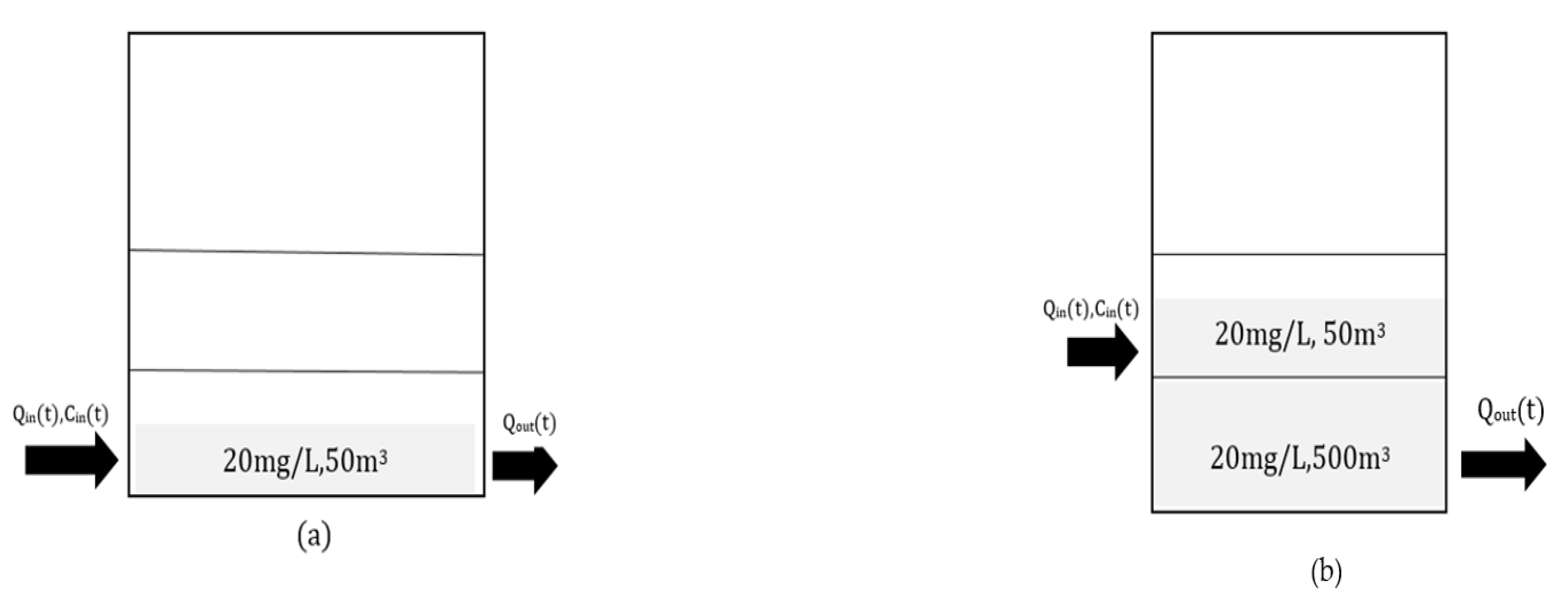
Figure 10.
(a) Both inlet and initial level of water in Compartment A; (b) inlet and initial level of water in Compartment B.
Figure 10.
(a) Both inlet and initial level of water in Compartment A; (b) inlet and initial level of water in Compartment B.

Figure 11.
Volume (m3) vs. time (h) for Compartments A, B, C in Figure 10. (a) Both inlet and initial level of water of Compartment A; (b) inlet and initial level of water of Compartment B, where VA(t) = volume of the water for Compartment A, VB(t) = volume of the water for Compartment B, and VC(t) = volume of the water for Compartment C.

Figure 12.
Concentration (mg/L) vs. time (h) for each compartment of Figure 10. (a) Both inlet and initial level of water of Compartment A; (b) inlet and initial level of water of Compartment B. CA(t) = concentration of the water for Compartment A, CB(t)= concentration of the water for Compartment B, CC(t) = concentration of the water for Compartment C.

Figure 13.
Different arrangement of initial conditions. (a) The inlet and initial level of water in Compartment A; (b) inlet point and initial level in Compartment B.
Figure 13.
Different arrangement of initial conditions. (a) The inlet and initial level of water in Compartment A; (b) inlet point and initial level in Compartment B.

Figure 14.
Volume (m3) vs. time (h) for Compartments A, B of Figure 13a,b, where VA(t) = volume of the water for Compartment A, VB(t) = volume of the water for Compartment B.
Figure 14.
Volume (m3) vs. time (h) for Compartments A, B of Figure 13a,b, where VA(t) = volume of the water for Compartment A, VB(t) = volume of the water for Compartment B.

Figure 15.
Concentration (mg/L) vs. time (hr) for each compartment of Figure 13a,b. CA(t) = concentration of the water for Compartment A, CB(t) = Concentration of the water for Compartment B.
Figure 15.
Concentration (mg/L) vs. time (hr) for each compartment of Figure 13a,b. CA(t) = concentration of the water for Compartment A, CB(t) = Concentration of the water for Compartment B.

Figure 16.
Numerical solution concentration (mg/L) vs. time (hr) for each compartment of Figure 10a and Figure 13a, where CA(t) = concentration of the water for Compartment A, CB(t) = concentration of the water for Compartment B, CC(t) = concentration of the water for Compartment C.

Figure 17.
Fluoride residuals at the outlet of Brushy Plains Tank using the model developed.

Figure 18.
Fluoride residuals at the outlet of the Brushy Plains Tank using the model developed and field data measurement results.
Figure 18.
Fluoride residuals at the outlet of the Brushy Plains Tank using the model developed and field data measurement results.


Table 1.
Multiple cases for three compartments during the filling stage.
| Level of Water | Compartment A | Compartment B | Compartment C | |||||||
|---|---|---|---|---|---|---|---|---|---|---|
| Inlet Point | ||||||||||
| Compartment A | A | B | C | A | B | C | A | B | C | |
| Case 1 | 0 | 0 | Case 2 | Case 3 | 0 | Case 4 | Case 5 | Case 6 | ||
| Compartment B | A | B | C | A | B | C | A | B | C | |
| Case 7 | 0 | 0 | Case 8 | Case 9 | 0 | Case 10 | Case 11 | Case 12 | ||
| Compartment C | A | B | C | A | B | C | A | B | C | |
| Case 13 | 0 | 0 | Case 14 | Case 15 | 0 | Case 16 | Case 16 | Case 18 | ||
Table 2.
Summary of the analytical solution during the filling stage.
| Level of Water | Compartment A | Compartment B | Compartment C | |||||||
|---|---|---|---|---|---|---|---|---|---|---|
| Inlet Point | ||||||||||
| Compartment A | A | B | C | A | B | C | A | B | C | |
| (8) | 0 | 0 | (12) | (16) | 0 | (12) | (20) | (24) | ||
| Compartment B | A | B | C | A | B | C | A | B | C | |
| (8) | 0 | 0 | C0A | (29) | 0 | C0A | (33) | (37) | ||
| Compartment C | A | B | C | A | B | C | A | B | C | |
| (8) | 0 | 0 | C0A | (29) | 0 | C0A | C0B | (41) | ||
Table 3.
List of cases for each compartment’s draining process, with varying inlets and inlet concentrations.
Table 3.
List of cases for each compartment’s draining process, with varying inlets and inlet concentrations.
| Level of Water | Compartment A | Compartment B | Compartment C | |||||||
|---|---|---|---|---|---|---|---|---|---|---|
| Inlet Point | ||||||||||
| Compartment A | A | B | C | A | B | C | A | B | C | |
| Case 1 | 0 | 0 | Case 2 | Case 3 | 0 | Case 4 | Case 5 | Case 6 | ||
Table 4.
Summary of the analytical solutions during the draining stage.
| Level of Water | Compartment A | Compartment B | Compartment C | |||||||
|---|---|---|---|---|---|---|---|---|---|---|
| Inlet Point | ||||||||||
| Compartment A | A | B | C | A | B | C | A | B | C | |
| C0A | 0 | 0 | (45) | C0B | 0 | (53) | (49) | C0C | ||
Table 5.
Map of the cases for filling each compartment, with different inlets and initial concentrations.
Table 5.
Map of the cases for filling each compartment, with different inlets and initial concentrations.
| Level of Water | Compartment A | Compartment B | |||
|---|---|---|---|---|---|
| Inlet Point | |||||
| Compartment A | A | B | A | B | |
| Case 1 | 0 | Case 2 | Case 3 | ||
| Compartment B | A | B | A | B | |
| Case 4 | 0 | Case 5 | Case 6 | ||
Table 6.
Summary of the analytical solution during the filling stage.
| Level of Water | Compartment A | Compartment B | |||
|---|---|---|---|---|---|
| Inlet Point | |||||
| Compartment A | A | B | A | B | |
| (60) | 0 | (64) | (68) | ||
| Compartment B | A | B | A | B | |
| (60) | 0 | C0Aexp(−kt) | (75) | ||
Table 7.
Map of the cases for draining of each compartment with different inlets and initial concentrations.
Table 7.
Map of the cases for draining of each compartment with different inlets and initial concentrations.
| Level of Water | Compartment A | Compartment B | |||
|---|---|---|---|---|---|
| Outlet Point | |||||
| Compartment A | A | B | A | B | |
| Case 1 | 0 | Case 2 | Case 3 | ||
Table 8.
Summary of the analytical solutions during the draining stage.
| Level of Water | Compartment A | Compartment B | |||
|---|---|---|---|---|---|
| Outlet Point | |||||
| Compartment A | A | B | A | B | |
| (79) | 0 | (87) | (83) | ||
Table 9.
Flow, Qin(t) [m3/h], and Qout(t) [m3/h] at each hour.
| Time (h) | 1 | 2 | 3 | 4 | 5 | 6 | 7 | 8 | 9 | 10 |
|---|---|---|---|---|---|---|---|---|---|---|
| Qin(t) [m3/h] | 200 | 0 | 120 | 90 | 250 | 0 | 0 | 120 | 0 | 200 |
| Qout(t) [m3/h] | 0 | 180 | 0 | 0 | 0 | 100 | 150 | 0 | 180 | 0 |
| Cin [mg/L] | 25 | 0 | 25 | 25 | 25 | 0 | 25 | 25 | 0 | 25 |
Publisher’s Note: MDPI stays neutral with regard to jurisdictional claims in published maps and institutional affiliations. |
© 2021 by the authors. Licensee MDPI, Basel, Switzerland. This article is an open access article distributed under the terms and conditions of the Creative Commons Attribution (CC BY) license (https://creativecommons.org/licenses/by/4.0/).
Share and Cite
MDPI and ACS Style
Abrha, B.; Ostfeld, A. Analytical Solutions to Conservative and Non-Conservative Water Quality Constituents in Water Distribution System Storage Tanks. Water 2021, 13, 3502. https://doi.org/10.3390/w13243502
AMA Style
Abrha B, Ostfeld A. Analytical Solutions to Conservative and Non-Conservative Water Quality Constituents in Water Distribution System Storage Tanks. Water. 2021; 13(24):3502. https://doi.org/10.3390/w13243502
Chicago/Turabian StyleAbrha, Biniam, and Avi Ostfeld. 2021. "Analytical Solutions to Conservative and Non-Conservative Water Quality Constituents in Water Distribution System Storage Tanks" Water 13, no. 24: 3502. https://doi.org/10.3390/w13243502
Note that from the first issue of 2016, this journal uses article numbers instead of page numbers. See further details here.