Spatiotemporal Changes in Temperature and Precipitation in West Africa. Part I: Analysis with the CMIP6 Historical Dataset

Abstract

Climate variability and change constitute major challenges for Africa, especially West Africa (WA), where an important increase in extreme climate events has been noticed. Therefore, it appears essential to analyze characteristics and trends of some key climatological parameters. Thus, this study addressed spatiotemporal variabilities and trends in regard to temperature and precipitation extremes by using 21 models of the Coupled Model Intercomparison Project version 6 (CMIP6) and 24 extreme indices from the Expert Team on Climate Change Detection and Indices (ETCCDI). First, the CMIP6 variables were evaluated with observations (CHIRPS, CHIRTS, and CRU) of the period 1983–2014; then, the extreme indices from 1950 to 2014 were computed. The innovative trend analysis (ITA), Sen’s slope, and Mann–Kendall tests were utilized to track down trends in the computed extreme climate indices. Increasing trends were observed for the maxima of daily maximum temperature (TXX) and daily minimum temperature (TXN) as well as the maximum and minimum of the minimum temperature (TNX and TNN). This upward trend of daily maximum temperature (Tmax) and daily minimum temperature (Tmin) was enhanced with a significant increase in warm days/nights (TX90p/TN90p) and a significantly decreasing trend in cool days/nights (TX10p/TN10p). The precipitation was widely variable over WA, with more than 85% of the total annual water in the study domain collected during the monsoon period. An upward trend in consecutive dry days (CDD) and a downward trend in consecutive wet days (CWD) influenced the annual total precipitation on wet days (PRCPTOT). The results also depicted an upward trend in SDII and R30mm, which, additionally to the trends of CDD and CWD, could be responsible for localized flood-like situations along the coastal areas. The study identified the 1970s dryness as well as the slight recovery of the 1990s, which it indicated occurred in 1992 over West Africa.

1. Introduction

Climate change is a widely known global phenomenon with varying impacts across regions. Its indicator is significant changes in human and natural systems [1,2]. Ref. [3] assessed the global surface temperature and found an increase approximately 0.07 °C/decade during the period 1901–2010 and about 0.17 °C per decade from 1979 to 2010. According to [4,5], this increase, which is higher in developing countries, is definitely due to both natural changes and changes observed in local change inputs (industrialization, transport, etc.). Extreme weather events induce a large range of effects on the environment and society and raise important challenges about environment and resource management for developing countries [6].

The African continent, according to [7,8], is the second most populous continent in the world. It is also one of the most vulnerable regions to climate variability and change because of its high exposure. Ref. [9] compared the periods 1995–2010 and 1979–1994 and noticed a significant increase in near-surface temperature anomalies over time. With its large latitudinal extent, Africa presents various climatologies, which vary widely. The northern and southern parts of Africa are known as the coolest areas of the continent. Studying the trend of temperature in North Africa, [10] found an increasing trend in the observed annual and seasonal mean surface temperatures. Further studies [11,12,13,14,15] confirmed for 21st-century projections an increase in the mean temperature in North Africa, the Middle East, and the Arabian Peninsula. This notification was in line with the fifth report of the Intergovernmental Panel on Climate Change (IPCC), which stressed that there was an increase in the number of extreme weather events for the 21st century due to climate change [16]. There is a strong link between temperature and precipitation because when temperatures rise, the amount of water vapor in the atmosphere also increases, and the spatiotemporal distributions of precipitation change, resulting in significant differences in precipitation across the world [17,18]. Therefore, obtaining real-time information and facilitating earlier predictions by decision makers can be an efficient tool to adapt and mitigate the impacts of climate events [19,20].

Investing in the present change and potential future change in West Africa (WA) is very useful and helpful because it is a region with unreliable monitoring networks and no or low climatological or meteorological surveys (institutional capacity). Various methods have been applied to investigate the region. They almost all refer to climate scenarios to provide a plausible explanation of how the future may evolve with respect to several variables, including socioeconomic change, technological change, energy and land use, and emissions of greenhouse gasses (GHGs) and air pollutants [21]. The IPCC, in its meeting in 2007, elaborated four levels of emission of trajectories relating to GHG concentrations called the Representative Concentration Pathway (RCP), which was projected by the IPCC in 2014. The RCPs are functions of a possible range of radiative forcing values (2.6, 4.5, 6.0, and 8.5 W/m²) up to the year 2100. On this basis, CMIP5 and CORDEX datasets were introduced into climate science research fields. These datasets, therefore, promoted various studies dedicated to the investigation of climate issues on the basis of the RCP projections. Some previous studies explored the CORDEX dataset [19,20,22,23,24,25,26,27] to investigate climate variability in Africa and West Africa, while other studies [28,29,30] examined the performance of the CMIP3/CMIP5 models in simulating extreme climate events. The latest dataset release, from the sixth assessment report of the IPCC, was the Coupled Model Intercomparison Project version 6 (CMIP6). This dataset was driven by a combination of two pathways of forcing, the Shared Socioeconomic Pathway (SSP) and Representative Concentration Pathway (RCP).

WA is one of the most vulnerable regions to climate variability and climate extreme events because of its limited capacity to adapt [8,19]. According to [31], WA, in the future, will be among the regions most highly impacted by climate change. The authors of [31], based on a review of 49 papers, revealed important changes in WA’s climate such as a reduction in the total annual rainfall (in both amount and length) as well as a rise in dry spells during the rainy season. Additionally, they expressed that the WA climate became warmer with important heatwave and spectacular drought episodes. These drought and heatwave episodes have been addressed over the study area by other authors such as those of [32,33,34,35,36]. Refs. [37,38] demonstrated that one of the most important components of the WA’s economy is agriculture, which is primarily rain-fed. The services sector dominates the WA economy, with a contribution of 42% of the GDP, followed by the agricultural sector, which inputs about 35% of the GDP [39].

Agricultural production in WA is uncertain, associated with between- and within-season rainfall variability, and remains a fundamental constraint to many investors, who often overestimate the negative impacts of climate-induced uncertainty [40]. WA has experienced important modifications since the droughts of the 1970s [36,41]. A rise in temperature and modification in rainfall (amount and spell duration) in WA have important implications on agriculture and water resource fields [42,43,44,45]. Regarding the projected change in the amounts and frequency of rainfall in WA [19,46,47], the uncertainty is considerably high, and several models do not agree on whether the change in rainfall will be negative or positive [48], especially for agriculture production. Ref. [49] explained that various studies on crops productivity over WA have shown that the impact of climate variability on crop yields is more frequently negative than positive. Thus, climate change impacts in the agriculture sector are a major challenge and need to be addressed. Some studies [20,50] have investigated adaptation strategies as a cornerstone to deal with sustainable agriculture [51] and climate change impacts [52]. It is important to understand whether the strategies are well designed and account for the best possible understanding of the trends of some parameters (e.g., precipitation and temperature). Using the CMIP6 dataset and referring to scenarios SSP1-2.6, SSP2-4.5, and SSP5-8.5, ref. [46] found that CMIP6 projected a continuous and significant increase in the mean annual temperature globally over all of Africa and subsequently over eight subregions of Africa during the 21st century. Meanwhile, ref. [53] adopted the same dataset to assess the representation of daily precipitation characteristics over West Africa and demonstrated how well CMIP6 reproduced observation patterns. However, these studies failed to investigate the trends in or frequency of precipitation and temperatures; they focused only on the variability of the parameters. The present study aimed to use the historical CMIP6 datasets (temperatures and precipitation) and analyze the trends of the changes in daily temperature and precipitation extremes over WA by calculating extreme climate index series, as well as using widely used and innovative statistical methods to assess the levels of changes. Section 2 of this paper, dedicated to the materials and methods, presents the study domain, the various datasets used, and the methodologies adopted, while the results and discussion are presented in Section 3 and Section 4, respectively. Finally, the conclusion in Section 5 summarizes the main findings of the study.

2. Materials and Methods

2.1. Study Domain

The study area lay in West Africa, which is located between latitudes 0° N and 25° N and longitudes 25° W and 25° E (Figure 1). The region is bordered in the South by the Gulf of Guinea and in the north by Mauritania, Mali, and Niger; the Cameroon highlands form the eastern boundary, while the Atlantic Ocean forms the western limit. Rainfall patterns over this region are mostly affected by ocean currents and local features such as topography. In terms of climatic zones, West Africa is divided into three different regions: the Sahel, which is characterized as a semiarid zone ranging from western Senegal to eastern Sudan, between 12° N and 20° N; the Sudano-Sahelian zone; and the Guinea coast, which is characterized by bimodality driven by the intertropical discontinuity (ITD).

2.2. Data

The model dataset utilized for the study was the Coupled Model Intercomparison Project 6th phase (CMIP6) database (precipitation and temperatures), and the observational datasets were CHIRPS, CHIRTS, and CRU. The CMIP6 historical dataset covers the period 1950–2014; CHIRPS covers 1981–present; CHIRTS, 1983–2016, and CRU, 1981–present.

2.2.1. Model CMIP6 Dataset

The datasets of the CMIP6 are divided into two phases (historical and projection) for all models used in the study. The datasets were published onto the ESGF data server and were freely accessed by searching the model name together with the reference ID (e.g., experiment name: “historical”, source: “model name”, variable: “pr”, “tasmax”, and “tasmin”) at https://esgf-data.dkrz.de/search/cmip6-dkrz/ (accessed on 18 June 2021), or https://esgfnode.llnl.gov/projects/cmip6/ (accessed on 18 June 2021). Datasets are stored in various formats, but we opted for the NetCDF format, which could be explored with almost all climate dataset visualization software (NCL, http://www.ncl.ucar.edu/, accessed on 18 June 2021) or Python (https://www.python.org/, accessed on 18 June 2021), R (https://cran.r-project.org/, accessed on 18 June 2021). A historical experiment dataset was available that included data from 1850 to 2014. For climate projection experiments, we used a combination of the Shared Socioeconomic Pathway (SSP) and Representative Concentration Pathway (RCP), which provide data for the period 2006–2300. In this study, the study period of interest for the calculation of the extreme climate indices was 1981–2014. The rainy season in West Africa is mainly related to the West African Monsoon, which oscillates between May and September (MJJAS) each year. The remaining months of the year were counted as participating in the so-called dry season. The CMIP6 models of interest have variable spatial resolutions and are illustrated in Table 1. In total, we used 21 CMIP6 models that made available both precipitation and temperature.

2.2.2. Observed CHIRPS, CHIRTS, and CRU Datasets

Because of a lack of ground-based observation data, scientists refer to satellite datasets as an alternative to supply in situ observations. To address this limitation, in the present study, rainfall data from the Climate Hazards Group Infrared Stations (CHIRPS) version 2, developed by the Climate Hazards Group of the University of California, was used (precipitation: https://data.chc.ucsb.edu/products/CHIRPS-2.0/africa_daily/, accessed on 2 May 2021). In the same line, its corresponding temperature (maximum and minimum) dataset, the Climate Hazards Group Infrared Temperature with Station data (CHIRTS), was adopted (CHIRTS: [37]; Temperatures: http://data.chc.ucsb.edu/products/CHIRTSdaily/v1.0/, accessed on 2 May 2021) along with the Climatic Research Unit Time Series (CRU: https://crudata.uea.ac.uk/cru/data/hrg/, accessed on 2 May 2021; precipitation and temperatures). The dataset was used at the daily time step. The CHIRPS dataset is a quasiglobal rainfall dataset covering 50° S–50° N, while CHIRTS covers 60° S–70° N. To be consistent with the simulation model periods, we adopted a CHIRXS (where X is indicated for precipitation or temperature) period of 1983–2014 under 0.25° × 0.25° (~25 km × 25 km) horizontal resolution.

The CRU and CHIRPS datasets have been widely used in previous studies [19,20,54] and provided satisfactory responses in respect to observational datasets (in situ). In the present work, both observed datasets (CHIRPS/CHIRTS and CRU) were used to first investigate the recent release (CHIRTS [55]) in response to maximum and minimum temperatures and then to see whether, as CHIRPS fits well with CRU (precipitation) CHIRTS could be a response to CRU (temperature).

2.3. Methods

Several studies have been conducted to date by scientists in designing methods and applications for the computation and analysis of extreme climate indices for better monitoring and tracking of climate trends. The methodology adopted in this study consisted of:

• analysis of the precipitation and the temperature recorded in the observational dataset;
• computation of the selected climate indices;
• analysis of the spatial trends of the extreme indices computed with modified Mann–Kendall and Sen’s slope tests;
• assessment of the performance of a new method (innovative trend analysis: ITA) in respect to that of the methods in iii.;
• analysis of the temporal variability and trend of the computed indices.

2.3.1. Selected Extreme Climate Event

The climate indices agreed with the international committee of the Expert Team on Climate Change Detection and Indices (ETCCDI), which aims to provide a good mixture of daily statistics to assess changes in temperature and precipitation regimes in terms of duration, intensity, and occurrence [56,57]. Based on the combination of CDO commands and the Climpact (https://climpact-sci.org/indices/, accessed on 13 May 2021), the extreme indices listed in Table 2 and Table 3 were calculated. The computed indices were classified into 5 sets of extremes climate indices: (i) absolute extreme indices—precipitation: RXnday (n = 1, n = 5, and n = 7), temperature: TXX, TXM, TMM, TNX, TNN, TNM, TXN; (ii) threshold exceedance indices such as R10mm, R20mm, and R30mm, which refer to the number of days on which a threshold was surpassed; (iii) indices that highlight the length of wet and dry spell duration, for instance, CDD and CWD; (iv) percentile-based precipitation and temperature indices (R95p, R99p, TN10p, TX10p, TN90p, TX90p, and WSDI); and (v) other indices—SDII and PRCPTOT.

2.3.2. Criteria of the Analysis of the Extremes

Some basic criteria were set to be accounted for in the analysis of the trend of each extreme climate event:

(a)

a minimum of 80% (17 models of 21) of the CMIP6 models needed to reflect the events or the trends;

(b)

a significant trend had to be demonstrated by at least 80% of the models.

2.3.3. Statistics Constraints to Evaluate the Performance of Models

The correlation analysis method was employed to evaluate the relationship between models and observations on one hand, and between indices on the other hand. Additionally, the nonparametric Mann–Kendall (MK) trend test [58,59], which is strongly recommended in this kind of analysis by the World Meteorological Organization (WMO), was adopted to evaluate the trends in extreme climate (both precipitation and temperature) indices. It was jointly associated with Sen’s slope test [60] for better appreciation of the trend. The aforementioned tests were all based on hypotheses. The null hypothesis (Ho) assumed that the data were independent and randomly distributed, and the alternative hypothesis (H1) supposed that there was a monotonic trend in the dataset. The utility of these two tests was that the MK test (with its Z Kendall coefficient) provided an idea about the significance of the trend, while Sen’s test (with the slope estimator) estimated the trend magnitude. The assessment was also based on a chosen 95% threshold of confidence level. An innovative trend analysis (ITA) was applied to detect monotonic trends and subtrends in the time-series dataset. This methodological approach was used to detect the annual and seasonal trends.

• Mann–Kendall test (MK)

MK [58,59] is one of the common formulas used in hydrology and meteorology to identify trends in a time-series dataset. The test statistic (S) of series ($x_1$, $x_2$, $x_3$, … and $x_n$) for which the trends are being checked can be expressed with the following formula:

$$S={\displaystyle \sum }_{k=1}^{n-1}{\displaystyle \sum }_{j=k+1}^{n}sign\left(x_j-x_k\right)$$

(1)

where n is the length of the dataset and $x_j$ and $x_k$ indicate the observations at times $j$ and $k$.

$$Sign\left(x_j-x_k\right)=\{\begin{array}{c}+1 if x_j>x_k\\ 0 if x_j=x_k\\ -1 if x_j<x_k\end{array}$$

(2)

A positive value for $S$ indicates an increasing or upward trend, while a negative value shows a decreasing or downward trend in the time-series data.

The variance of S, VAR(S), can be calculated by the equation:

$$VAR\left(S\right)=\frac{1}{18}\left\{n\left(n-1\right)\left(2n+5\right)-{\displaystyle \sum }_{i=1}^{\rho }{\tau }_i\left({\tau }_i-1\right)\left(2{\tau }_i+5\right)\right\}$$

(3)

where $\rho$ denotes the tied group number of observations in group I, which is a set of sample data with similar values, and $i$ indicates the extent of the $i\mathrm{th}$ tie number.

The time-series data statistic (S) is identified with Kendall’s $\tau$ (tau), which is given as follows:

$$\tau =\frac{S}{B}$$

with, $B=\sqrt{\frac{1}{2}n\left(n-1\right)-\frac{1}{2}{{\displaystyle \sum }}_{j=1}^g{\rho }_j\left({\rho }_j-1\right)}$ $\sqrt{\frac{1}{2}n\left(n-1\right)}$.

Through the estimation of S and the variance VAR(S), the standardized test measurement Z is as follows when n > 10 [61]:

$$Z=\{\begin{array}{c}\frac{S-1}{\sqrt{VAR\left(S\right)}},if S>0\\ 0,if S=0\\ \frac{S+1}{\sqrt{VAR\left(S\right)}},if S<0\end{array}$$

(4)

The positive (+) values of Z indicate an increasing trend, and the negative (−) values depict a decreasing trend.

• Modified Mann–Kendall test (MMK)

From [62], modified VAR(S) statistics can be estimated with the equation:

$$VAR\left(S\right)=\left(\frac{n\left(n-1\right)\left(2n+5\right)}{18}\right).\left(\frac{n}{n_e^{*}}\right)$$

(5)

Here, the correction factor $\left(\frac{n}{n_e^{*}}\right)$ is adjusted to the autocorrelated data as:

$$\left(\frac{n}{n_e^{*}}\right)=1+\left(\frac{2}{n^3-3n^2+2n}\right){\displaystyle \sum }_{f=1}^{n-1}\left(n-f\right)\left(n-f-1\right)\left(n-f-2\right){\rho }_e\left(f\right)$$

(6)

${\rho }_e\left(f\right)$ signifies the autocorrelation between ranks of observations and can be estimated as:

$$\rho \left(f\right)=2sin\left(\frac{\pi }{6}\right){\rho }_e\left(f\right)$$

(7)

• Sen’s Slope Estimator

The Sen’s slope $\left(Q\right)$ is the median of N values of $Q_i$ [63], where

$$Q_i=\frac{x_k-x_j}{k-j},i=1,2,3,\dots ,N,k>j$$

(8)

Thus if some zero values of $Q_i$ fall in between equal numbers of negative and positive values of $Q_i$, the Sen’s slope (Q) is zero. The greater the number of equal values there are in a time series, the higher the probability of a no-change trend for the series [64].

• Innovative Trend Analysis (ITA)

One recent method proposed for hydroclimatic variability assessment is innovative trend analysis (ITA), which was first elaborated in [65]. This new and robust technique is used in hydrometeorology for trend detection. It has been applied for different variables such as groundwater, rainfall, temperature, and evapotranspiration [66,67]. The methodology consists of dividing into two subseries of equal numbers in the observation variables of the study. For the next step, each subseries is reorganized in ascending order and plotted against the other in a Cartesian coordinate system [68]. The first half is plotted on the X-axis, and the second half on the Y-axis. After that, a straight line is fitted with the scatter plot that represents the “monotonic trend “or so-called “no trend”. When the scatter is concentrated above the 1:1 line, the time series has an increasing trend, and if the scatter points concentrate below the line (1:1), a decreasing trend in the time series is indicated [69]. The trend indicator of ITA [65] is calculated from the following equation:

$$B=\frac{1}{n}{\displaystyle \sum }_{i=1}^n\frac{10\left(x_j-x_k\right)}{\overline{x}}$$

(9)

where B represents the ITA slope, n denotes the extent of individual subseries, $x_j$ and $x_k$ represent the values of the consecutive subseries, and x represents the mean of the first subseries ($x_k$).

Table 1. Reference of CMIP6 dataset used in this study.

N°	Models	Institute	Horizontal Resolution	References
1	ACCESS-CM2	Commonwealth Scientific and Industrial Research Organization, Australia Bureau of Meteorology (BoM), Australia	1.9° × 1.3°	[70]
2	ACCESS-ESM1-5	Commonwealth Scientific and Industrial Research Organization, Australia	1.9° × 1.2°	[71]
3	AWI-ESM-1-1-LR	Alfred Wegener Institute, Helmholtz Centre for Polar and Marine Research, Germany	1.9° × 1.9°	[72]
4	BCC_ESM1	Beijing Climate Centre (BCC) and China Meteorological Administration (CMA), China	2.8° × 2.8°	[73]
5	CanESM5	Canadian Earth System Model, Canada	2.8° × 2.8°	[74]
6	EC_EARTH3-VEG-LR	EC—Earth Consortium, Rossby Center, Swedish Meteorological and Hydrological Institute (SMHI), Sweden	0.7° × 0.7°	Not available
7	EC_EARTH3-CC	EC—Earth Consortium, Rossby Center, SMHI, Sweden	0.7°× 0.7°	[75]
8	FGOALS_f3_L	LASG, Institute of Atmospheric Physics, Chinese Academy of Sciences and CESS, Tsinghua University, China	1.3° × 1.0°	[76]
9	FGOALS_g3	LASG, Institute of Atmospheric Physics, Chinese Academy of Sciences and CESS, Tsinghua University, China	2.0° × 2.3°	[77]
10	IPSL-CM6A-LR	Institut Pierre-Simon Laplace (IPSL), France	2.5° × 1.3°	[78]
11	MIROC6	Japan Agency for Marine–Earth Science and Technology; Atmosphere and Ocean Research Institute (University of Tokyo); and National Institute for Environmental Studies, Japan	1.4° × 1.4°	[79]
12	MPI-ESM-1-2-HAM	Max Planck Institute for Meteorology, Germany	1.9° × 1.9°	[80]
13	MPI_ESM1_2_HR	Max Planck Institute for Meteorology, Germany	0.9° × 0.9°	[81]
14	MPI_ESM1_2_LR	Max Planck Institute for Meteorology, Germany	1.9° × 1.9°	[82]
15	MRI_ESM2_0	Meteorological Research Institute (MRI), Japan	1.1° × 1.1°	[83]
16	NESM3	Nanjing University of Information Science and Technology, China	1.9° × 1.9°	[84]
17	NorCPM1	NorESM Climate modeling Consortium consisting, Norway	2.5° × 1.9°	[85]
18	NorESM2_MM	Norwegian Climate Center, Norway	1.3° × 0.9°	[86]
19	NorESM2-LM	Norwegian Climate Center, Norway		[87]
20	SAMO_UNICON	Seoul National University Atmosphere Model Version 0 with a Unified Convection Scheme, South Korea	1.2° × 0.9°	[88]
21	TaiESM1	Research Center for Environmental Changes (AS-RCEC), Taiwan	0.9° × 1.3°	[89]

Table 1. Reference of CMIP6 dataset used in this study.

N°	Models	Institute	Horizontal Resolution	References
1	ACCESS-CM2	Commonwealth Scientific and Industrial Research Organization, Australia Bureau of Meteorology (BoM), Australia	1.9° × 1.3°	[70]
2	ACCESS-ESM1-5	Commonwealth Scientific and Industrial Research Organization, Australia	1.9° × 1.2°	[71]
3	AWI-ESM-1-1-LR	Alfred Wegener Institute, Helmholtz Centre for Polar and Marine Research, Germany	1.9° × 1.9°	[72]
4	BCC_ESM1	Beijing Climate Centre (BCC) and China Meteorological Administration (CMA), China	2.8° × 2.8°	[73]
5	CanESM5	Canadian Earth System Model, Canada	2.8° × 2.8°	[74]
6	EC_EARTH3-VEG-LR	EC—Earth Consortium, Rossby Center, Swedish Meteorological and Hydrological Institute (SMHI), Sweden	0.7° × 0.7°	Not available
7	EC_EARTH3-CC	EC—Earth Consortium, Rossby Center, SMHI, Sweden	0.7°× 0.7°	[75]
8	FGOALS_f3_L	LASG, Institute of Atmospheric Physics, Chinese Academy of Sciences and CESS, Tsinghua University, China	1.3° × 1.0°	[76]
9	FGOALS_g3	LASG, Institute of Atmospheric Physics, Chinese Academy of Sciences and CESS, Tsinghua University, China	2.0° × 2.3°	[77]
10	IPSL-CM6A-LR	Institut Pierre-Simon Laplace (IPSL), France	2.5° × 1.3°	[78]
11	MIROC6	Japan Agency for Marine–Earth Science and Technology; Atmosphere and Ocean Research Institute (University of Tokyo); and National Institute for Environmental Studies, Japan	1.4° × 1.4°	[79]
12	MPI-ESM-1-2-HAM	Max Planck Institute for Meteorology, Germany	1.9° × 1.9°	[80]
13	MPI_ESM1_2_HR	Max Planck Institute for Meteorology, Germany	0.9° × 0.9°	[81]
14	MPI_ESM1_2_LR	Max Planck Institute for Meteorology, Germany	1.9° × 1.9°	[82]
15	MRI_ESM2_0	Meteorological Research Institute (MRI), Japan	1.1° × 1.1°	[83]
16	NESM3	Nanjing University of Information Science and Technology, China	1.9° × 1.9°	[84]
17	NorCPM1	NorESM Climate modeling Consortium consisting, Norway	2.5° × 1.9°	[85]
18	NorESM2_MM	Norwegian Climate Center, Norway	1.3° × 0.9°	[86]
19	NorESM2-LM	Norwegian Climate Center, Norway		[87]
20	SAMO_UNICON	Seoul National University Atmosphere Model Version 0 with a Unified Convection Scheme, South Korea	1.2° × 0.9°	[88]
21	TaiESM1	Research Center for Environmental Changes (AS-RCEC), Taiwan	0.9° × 1.3°	[89]

Table 2. Precipitation extreme indices.

Index	Description Name	Definition	Units
R95p	Very wet day precipitation	Annual total precipitation when RR > 95th percentile	mm
R99p	Extremely wet day precipitation	Annual total precipitation when RR > 99th percentile	mm
Rx1day	Maximum 1-day precipitation	Annual maximum 1-day precipitation	mm
Rx5day	Maximum 5-day precipitation	Annual maximum consecutive 5-day precipitation	mm
Rx7day	Maximum 7-day precipitation	Annual maximum consecutive 7-day precipitation	mm
PRCPTOT	Wet day precipitation	Annual total precipitation on wet days	mm
SDII	Simple daily intensity index	Average precipitation on wet days	mm/day
CDD	Consecutive dry days	Maximum number of consecutive dry days	day
CWD	Consecutive wet days	Maximum number of consecutive wet days	day
R10mm	Number of heavy precipitation days	Annual count of days when RR > 10 mm	day
R20mm	Number of very heavy precipitation days	Annual count of days when RR > 20 mm	day
R30mm	Number of heaviest precipitation days	Annual count of days when RR > 30 mm	day

Table 2. Precipitation extreme indices.

Index	Description Name	Definition	Units
R95p	Very wet day precipitation	Annual total precipitation when RR > 95th percentile	mm
R99p	Extremely wet day precipitation	Annual total precipitation when RR > 99th percentile	mm
Rx1day	Maximum 1-day precipitation	Annual maximum 1-day precipitation	mm
Rx5day	Maximum 5-day precipitation	Annual maximum consecutive 5-day precipitation	mm
Rx7day	Maximum 7-day precipitation	Annual maximum consecutive 7-day precipitation	mm
PRCPTOT	Wet day precipitation	Annual total precipitation on wet days	mm
SDII	Simple daily intensity index	Average precipitation on wet days	mm/day
CDD	Consecutive dry days	Maximum number of consecutive dry days	day
CWD	Consecutive wet days	Maximum number of consecutive wet days	day
R10mm	Number of heavy precipitation days	Annual count of days when RR > 10 mm	day
R20mm	Number of very heavy precipitation days	Annual count of days when RR > 20 mm	day
R30mm	Number of heaviest precipitation days	Annual count of days when RR > 30 mm	day

Table 3. Temperature extreme indices.

Index	Description Name	Definition	Units
TXM	Annual mean TX	Arithmetic mean of the monthly mean value of TX	°C
TNM	Annual mean TN	Arithmetic mean of the monthly mean value of TN	°C
TXX	The maximum value of TX	Highest TX in a year	°C
TNX	The maximum value of TN	Highest TN in a year	°C
TXN	The minimum value of TX	Lowest TX in a year	°C
TNN	The minimum value of TN	Lowest TN in a year	°C
TN10p	Cold nights	Percentage of days when TN < 10th percentile	%
TX10p	Cold days	Percentage of days when TX < 10th percentile	%
TN90p	Warm nights	Percentage of days when TN > 90th percentile	%
TX90p	Warm days	Percentage of days when TX > 90th percentile	%
WSDI	Warm spell duration index	Annual count of when at least six consecutive days of maximum temperature >90th percentile	day
CSDI	Cold spell duration index	Annual count of when at least six consecutive days of minimum temperature < 10th percentile	day

Table 3. Temperature extreme indices.

Index	Description Name	Definition	Units
TXM	Annual mean TX	Arithmetic mean of the monthly mean value of TX	°C
TNM	Annual mean TN	Arithmetic mean of the monthly mean value of TN	°C
TXX	The maximum value of TX	Highest TX in a year	°C
TNX	The maximum value of TN	Highest TN in a year	°C
TXN	The minimum value of TX	Lowest TX in a year	°C
TNN	The minimum value of TN	Lowest TN in a year	°C
TN10p	Cold nights	Percentage of days when TN < 10th percentile	%
TX10p	Cold days	Percentage of days when TX < 10th percentile	%
TN90p	Warm nights	Percentage of days when TN > 90th percentile	%
TX90p	Warm days	Percentage of days when TX > 90th percentile	%
WSDI	Warm spell duration index	Annual count of when at least six consecutive days of maximum temperature >90th percentile	day
CSDI	Cold spell duration index	Annual count of when at least six consecutive days of minimum temperature < 10th percentile	day

A positive slope of the B value indicates an increasing trend in the series, whereas a negative value of the slope signifies a decreasing tendency in the time series.

3. Results

This section focuses on presenting the main findings of the study. It depicts rainfall and temperature variabilities using selected climate indices over the study area and reports our analysis of their various trends with statistical tests. The reader is invited to see the supplementary documentation for additional figures and tables that are not shown here.

3.1. Scenario Models Validation

Validation of the CMIP6 models used was undertaken with observed rainfall and temperature (maximum and minimum) for the two databases in the period 1983–2014.

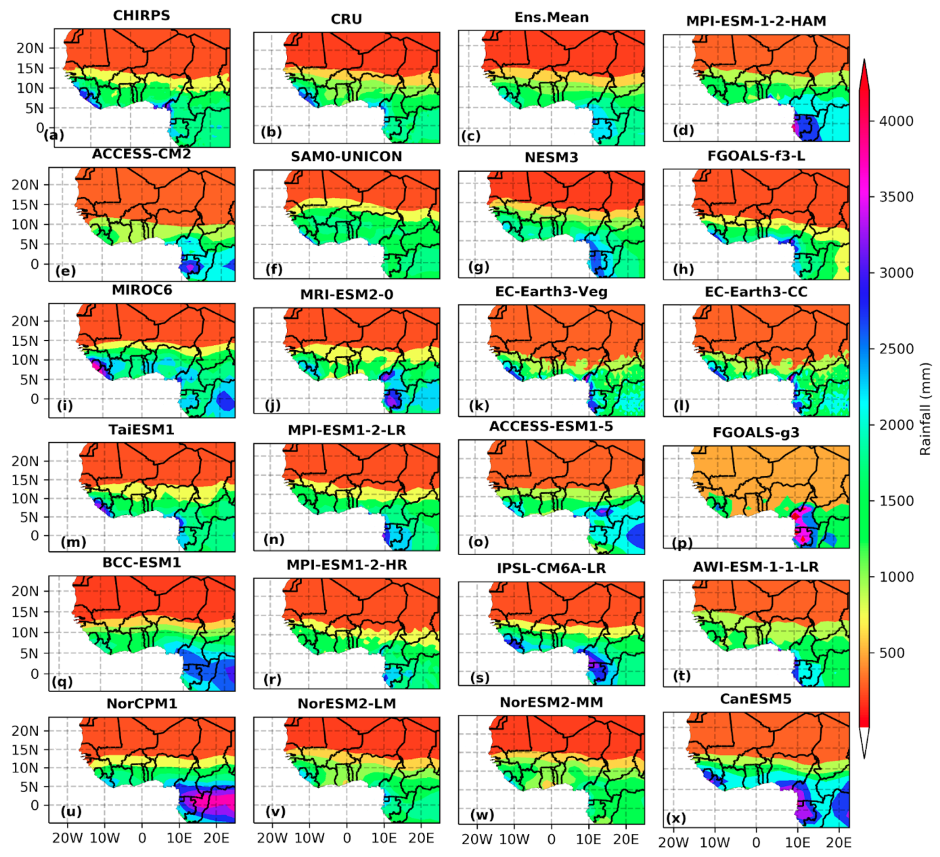
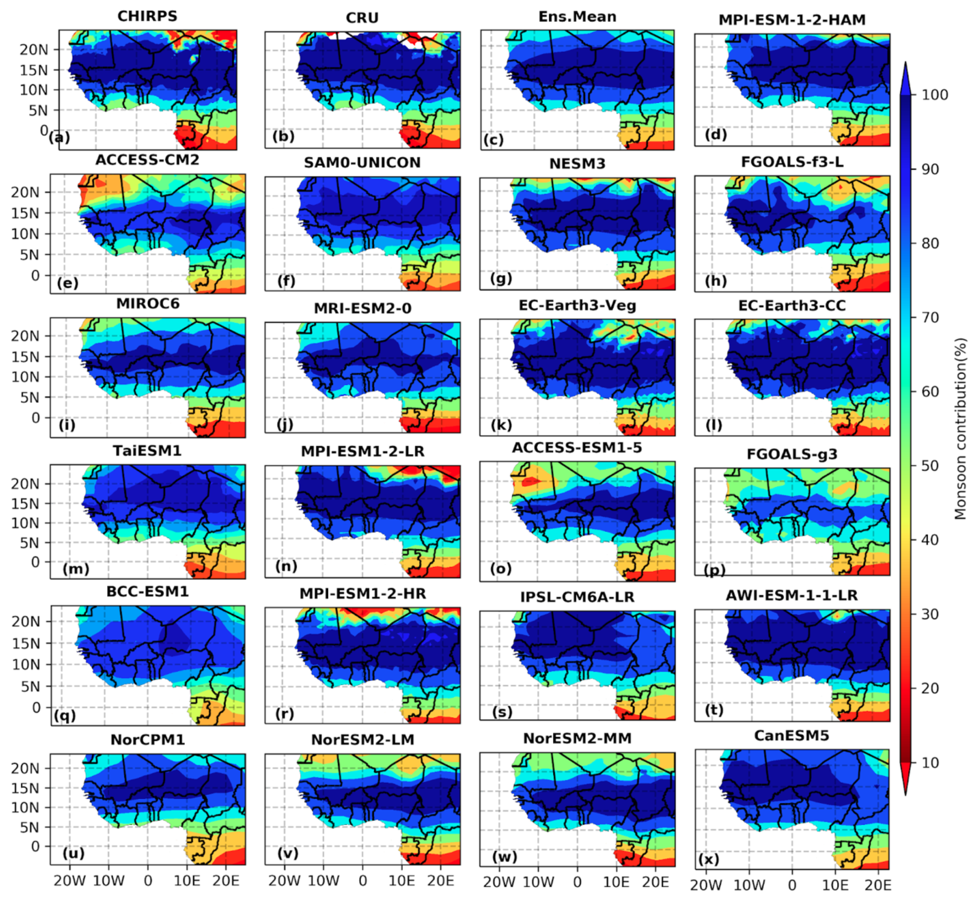
3.1.1. Rainfall Evaluation

Figure 2 shows the interannual distribution of rainfall averages for both the CMIP6 (21 models) and observed (CRU and CHIRPS) data as well as for the ensemble mean of the models. It can be seen that the total annual rainfall varied greatly across the study domain. For all the models and observations, there existed a northward gradient from higher to lower values, with the highest values recorded over the Guinea Highlands and Cameroon mountains (about 2500 mm/year for the observed and 2000 mm/year for the model ensemble mean). The Savannah region was generally wet, with a rainfall of about 700 mm/year. For the northern part, the rainfall recorded was less than 400 mm/year, and for the southern part (around the Guinea Coast), it was about 1100 mm to 1300 mm per year. Some models (ASSECC-ESM1-5, EC-Earth3-Veg, EC-Earth3-CC, FGOAL-g3, etc.) underestimated the rainfall compared with both observations (CHIRPS and CRU) and the model ensemble average. Other models (MPI-ESM-1-2-HAM, FGOAL-g3, MRI-ESM2-0, etc.) overestimated (especially in regions such as Cameroon’s mounts and Gabon’s forests) the observed rainfall datasets.

The rainfall recorded during the monsoon period (MJJAS) over the study domain is depicted in supplementary material (Figure S2). As in the case of the annual rainfall average, a northward gradient was noted, with the maximum and minimum of rainfall recorded over the same locations. A high correlation of models with observations was noted at latitude 5° N–20° N. The maximum cumulative rainfall registered during the monsoon period was about 2000 mm/year.

Figure 3 presents the average percentage of the contribution of the monsoon to the annual total mean. The monsoon contributed significantly to the total rainfall in the Savannah region (even underestimating models confirmed this observation). Between the latitudes 5° N and 20° N, at least 85% of the rainfall amount was received during May–September. It was also observed that the West African Monsoon did not contribute to rainfall above 25° N or below the equator.

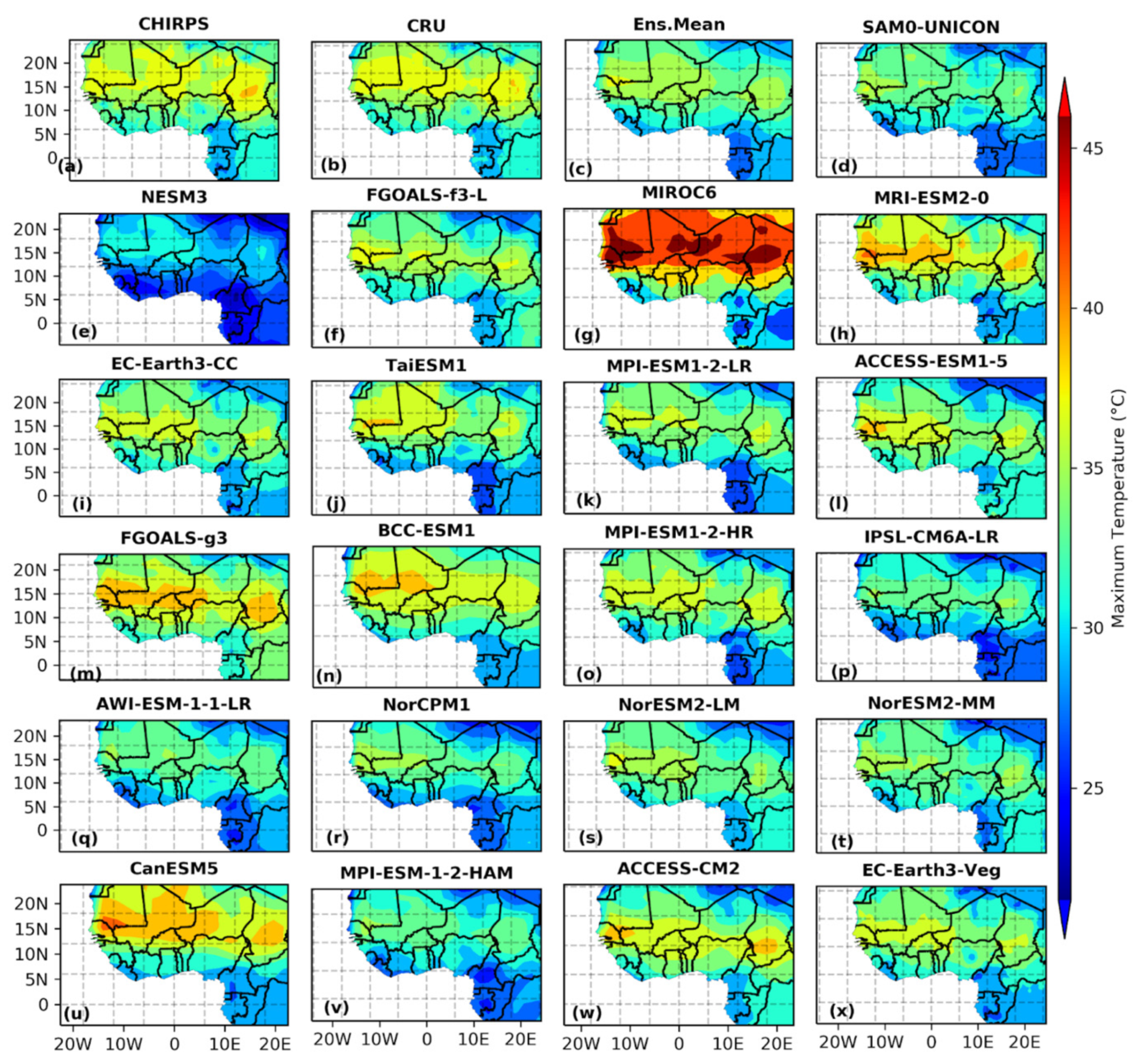
3.1.2. Temperatures Evaluation

The assessment of the maximum and minimum temperatures (Tmax and Tmin respectively) revealed that, for observations as well as models, the temperatures varied widely. Models differently represented the temperature, both for Tmax (Figure 4) and Tmin (Figure S2). All the minima of Tmin were located in the northern part, especially in the northeastern area, while the maxima of the Tmin were captured in the western region; the other parts were, on average, 22 ± 3 °C. For the Tmax, some models underestimated the observations (NESM3, SAMO-UNICON, IPSL-CM6A-LR, etc.) while others overestimated (MIROC6, CanESM5, BCC-ESM1). The lowest values of Tmax were located in the northeastern regions (as in the case of the minimum of the Tmin) and scattered around Cameroon’s mountains and Gabon’s forests. Each model, whether over- or underestimating, agreed that the hottest area was the Savannah’s band, located at the borders of Mali, Mauritania, and Senegal. The models’ ensemble mean was closer to the annual average of CRU than CHIRPS and depicted the observations better than the individual models. This means that the models’ ensemble provided a better estimate of the parameters than the individual models.

3.2. Interannual Rainfall and Temperatures Trend

To study the trends in the selected CMIP6 models, the work investigated the historical period 1950–2014, for which both precipitation and temperature data were available. To assess the annual rainfall and temperature trend, an advanced graphical method of trend detection was applied that included innovative trend analysis (ITA), the modified Mann–Kendall test (MMK), and Sen’s slope.

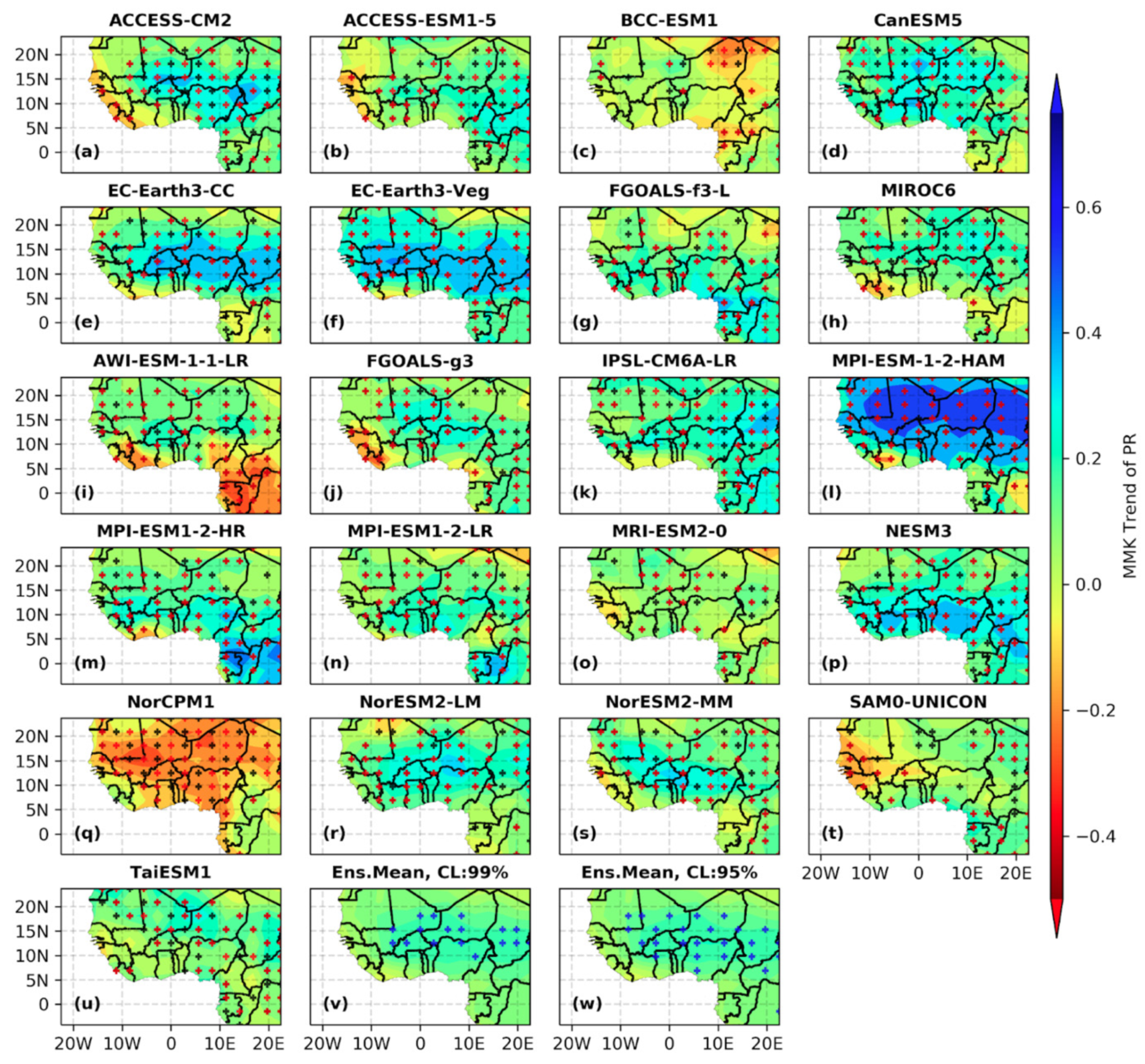
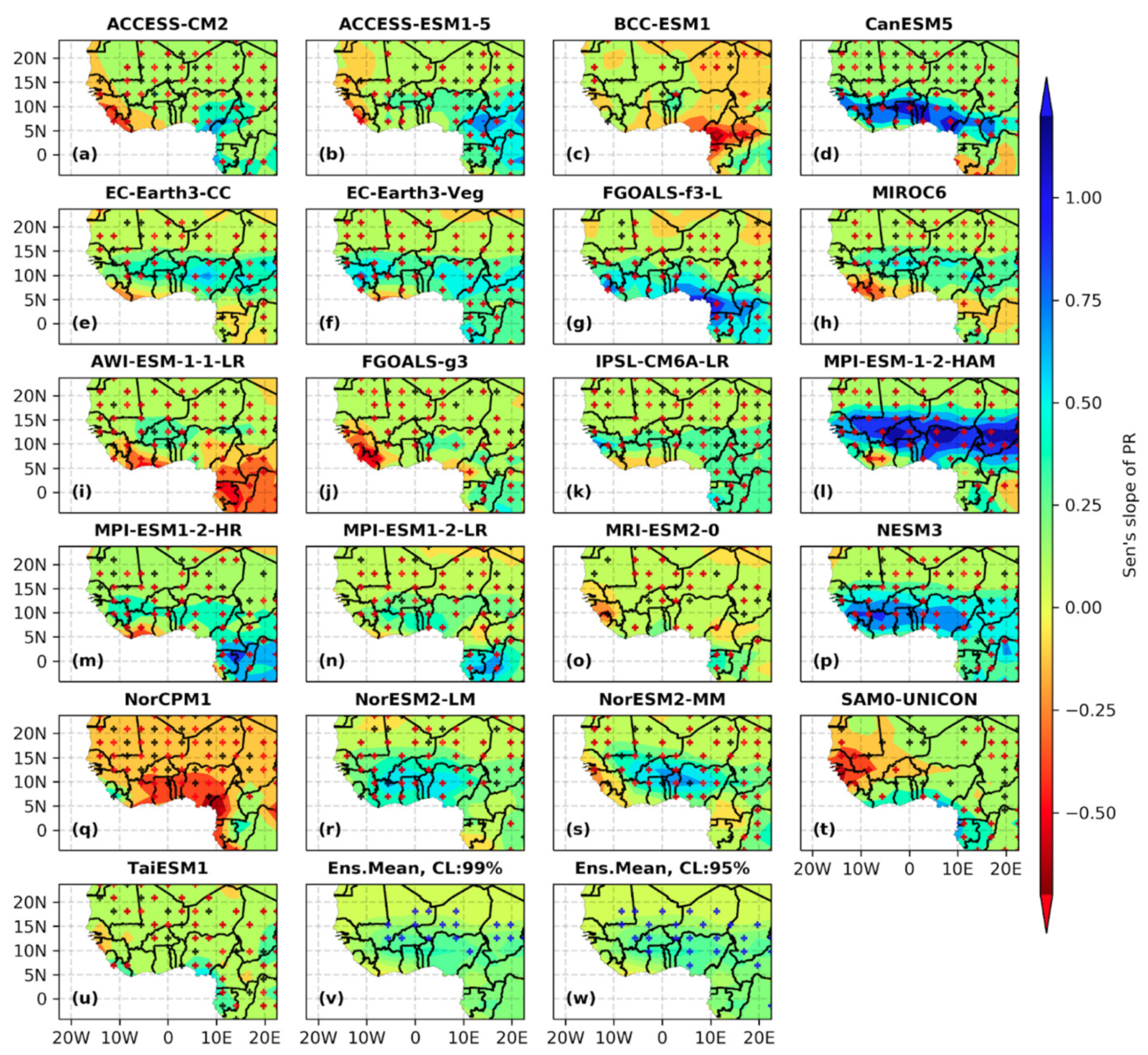
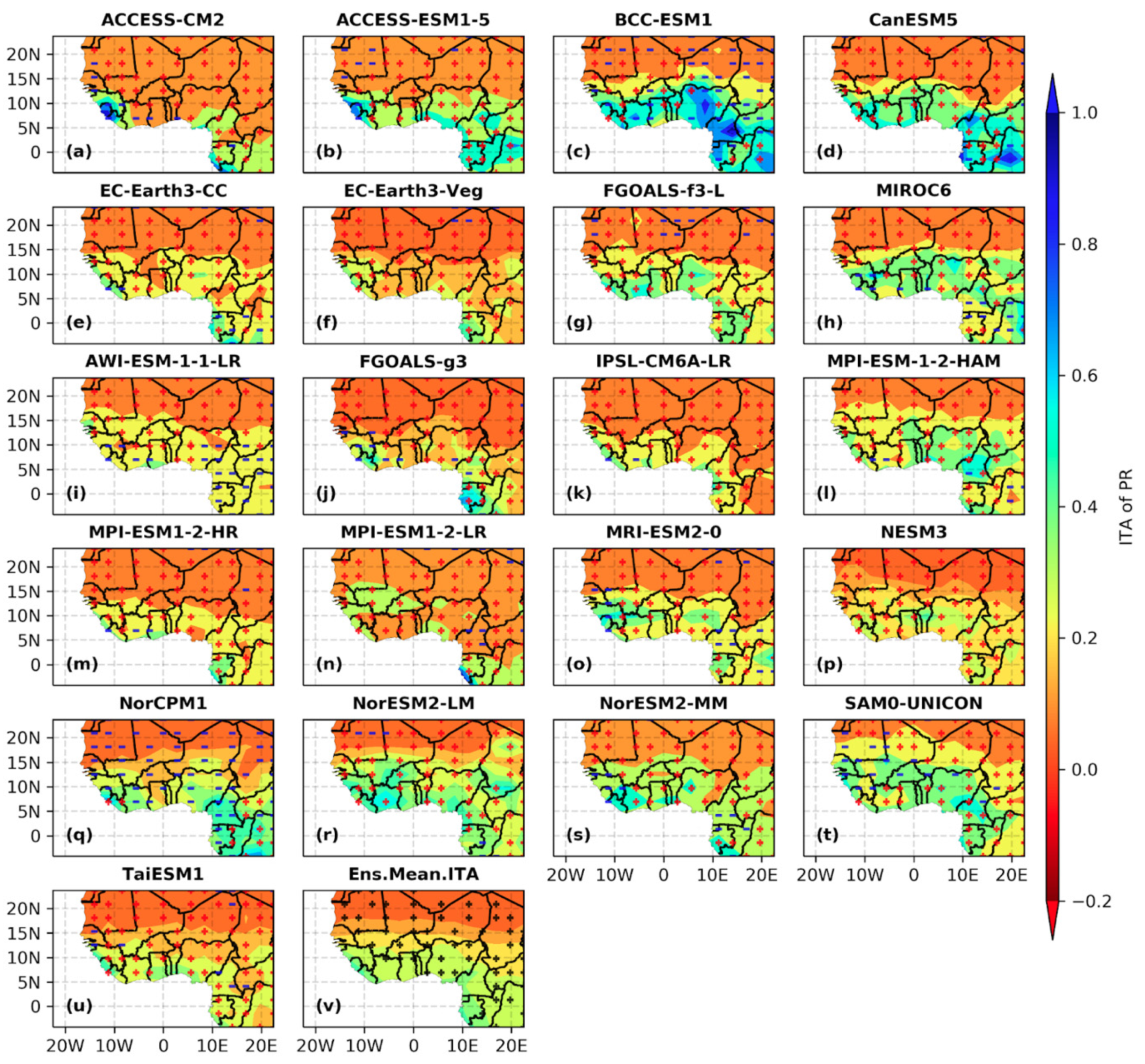
3.2.1. Trend of Annual Rainfall

Figure 5, depicting the evaluation with the MMK test, shows, based on its corrected Z statistic (Zc) that the trend of the rainfall varied from one model to another. From Figure 5a–u, the red cross indicates where trends were significant at 99% confidence level (CL), and the black cross indicates where trends were significant at at 95% CL. Globally, all the models indicated significant (either 95% or 99% of CL) positive trends; nonsignificant negative trends of annual rainfall were noticed over the Guinea Highlands (reduction of about 4–5 mm/decade) and some other parts, such as Cameroon.

The Savannah region experienced a significant increase in annual rainfall. In most locations in the study domain, a significant decreasing trend in annual rainfall was evident over Cameroon and Gabon, particularly in models such as AWI-ESM-1-1-LR, BCC-ESM1, NorCPM1; other models showed an increase in the yearly rainfall for these areas. In Figure 5v, the blue crosses indicate where at least 80% of the models depicted a trend with 99% CL, while in Figure 5w, the blue crosses express where at least 80% of models depicted a trend with 95% CL. The subplots Figure 5v,w indicated globally that, for the CMIP6 models studied, the Savannah showed a maximum rate of a significant increase in annual rainfall (about 4–5 mm/decade). A severe decline (nonsignificant) was identified around the Guinea Highlands but was revealed by less than 80% of the considered models.

The same trends were observed from the results of Sen’s slope test (Figure 6) as from the MMK results (Figure 5). The trends were located in the same areas and differed only in magnitude. The yearly reduction in rainfall around the Guinea highlands here was about 0.2–0.5 mm, while the global increase noted reduced by 5 mm/decade. The yearly variability (average increasing) of the rainfall over West Africa was about 3 mm/decade, but around the Savannah, Sen’s slope indicated a significant upward trend of about 4.5 mm/decade of at least at 95% CL under a minimum of 80% of the studied models.

The evaluation of the annual rainfall trend by applying the ITA is presented in Figure 7. In Figure 7a–u, the red crosses (+) express increasing trends, and the blue minuses (−) decreasing trends. The spatial distribution of the ITA trend indicator displayed the same variabilities and trends as did Sen’s slope (Figure 6) and MMK (Figure 5) trend analysis. On one hand, declining trends circulated over the extreme western part of WA (Guinea highlands) and were shown by at least 80% of the models. On the other hand, about 60% of the models revealed that the Cameroon mountains and Gabon forests exhibited the same declining trends. Generally, the rest of the WA domain experienced a stable increasing trend. The trends highlighted were all significant, at least at 95% CL. Additionally, a few significant trends ignored by MMK and Sen’s slope could be identified here, justifying the reliability of ITA to track unseen trends in time-series data. Furthermore, the identified trends from Sen’s slope and MMK were increased in magnitude under ITA. The maximum amount of the trend for ITA was about 10 mm/decade and was very high between the latitudes of 5° N and 15° N. In the northern part of WA, the trend indicator expressed a decrease of about +2 mm/decade.

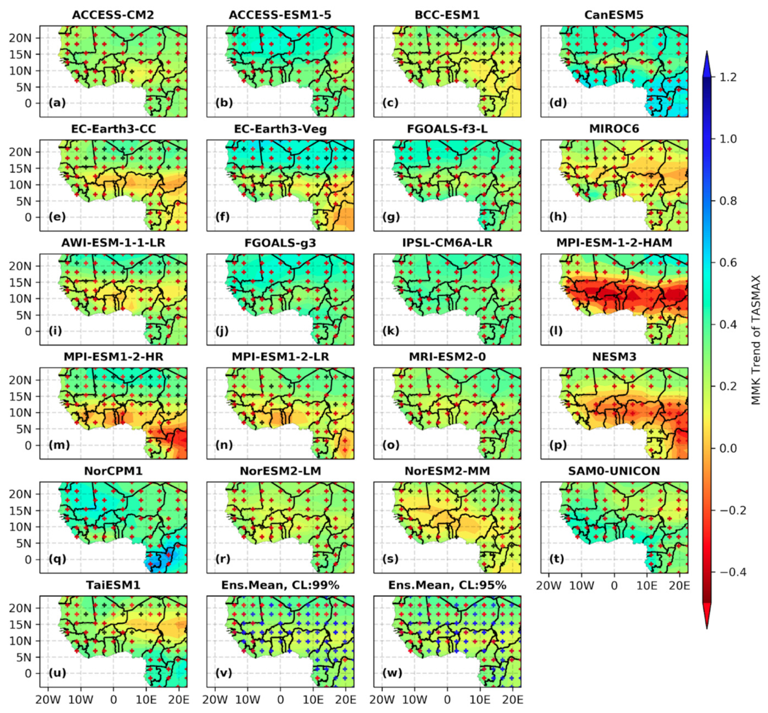
3.2.2. Trend of Maximum and Minimum Temperatures

Figure 8 and Figure 9 display trend analyses of the maximum temperatures of the selected CMIP6 dataset over the period 1950–2014 based on Sen’s slope and the Mann–Kendall test, respectively (Figures S3–S6 depict the Sen’s slope of Tmin, the MMK of Tmin, the ITA of Tmax, and the ITA of Tmin, respectively). It was perceived that the interannual variabilities of Tmin and Tmax were significant at least at 95% CL (red crosses indicate significant trends at 99% CL, and black crosses those at 95% CL) for all models.

The Z statistic score, the Sen’s slope, and the ITA slope, as well as the latter’s indicator, express how much the changes have impacted WA. For the Savannah regions, almost 90% of models showed change trends, but not with the same magnitude; only NESM3, MPI-ESM-1-2-HAM, and MPI-ESM1-2-HR behaved differently under the Sen’s and MMK tests. For ITA, however, the trend was dynamically elaborated, showing, for instance, in the case of the aforementioned models, on one hand, a clear increasing trend (northward from Savannah: 0.6 mm/year), and on another hand, a southward decreasing trend for both Tmin and Tmax.

Generally, for either Tmax or Tmin, there was a significant increasing trend across WA with a northward gradient. The northern part grew hotter than the central and the southern parts. ITA revealed (Figure 9v) that all the models (red cross locations) identified a particular increasing trend in the northern part and the Guinea-coast. The increasing trends around the Guinea coast could be due to the gradual increase in sea surface temperature (SST) due to global warming [90].

3.3. Spatial Changes in Temperature Indices

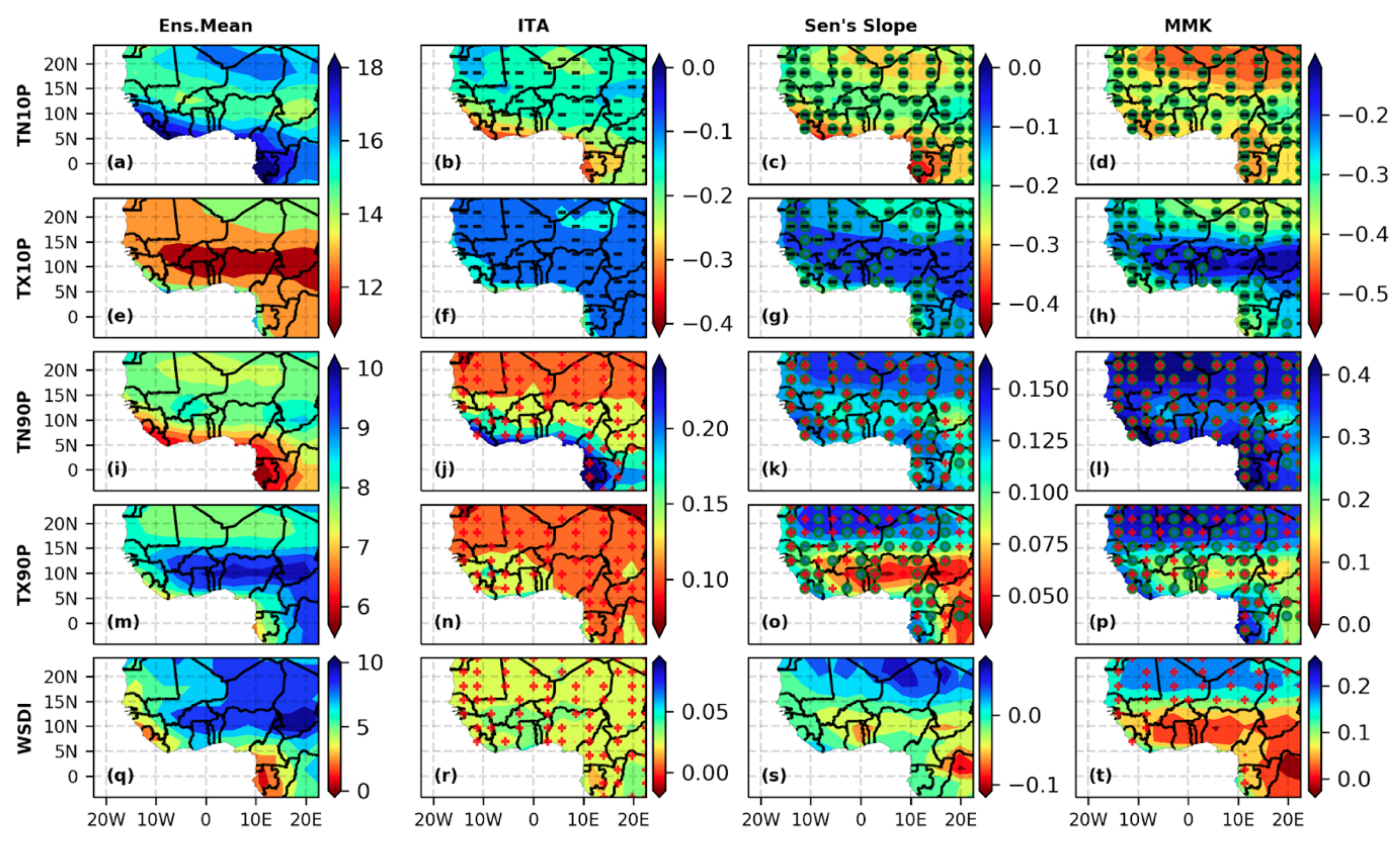
3.3.1. Percentile-Based Temperature Indices (TN10p, TX10p, TN90p, TX90p, and WSDI)

Figure 10 shows the spatial distribution of the cold indices (and warm indices) such as TX10p and TN10p (and TX90p and TN90p). The cold indices showed a significant decreasing trend (99% CL) under all the methods applied. For the cool day frequency (TX10p), the decline was about 2 days to 3 days/decade from Savannah–Sahel to the GC under the MMK and about 1 day/decade under the ITA and Sen’s slope methods. The reduction in cool days per year was important in the Sahel with a diminution of about 3 to 3.7 days/decade under the MMK trend test and about 1.8 days/decade under the Sen’s slope and ITA trend tests. The cold night days were more important over the GC (about 17 days/year) than the rest of the domain; fewer cold nights were over the Savannah. Cold nights per year also decreased in trend over the whole domain, with the maximum decrease across the GC (−3 days/decade under ITA and the Sen’s slope and −4 days/decade under MMK) and the northern part (−3 days/decade under Sen’s slope, −4.5 days/decade under MMK, and −2 days/decade under ITA). Additionally, the cold spell duration indicator (CSDI) during the study period (1950–2014) was high along the GC (27 days/year) and the northeastern part (23 days/year), with an obvious decreasing trend under all three analysis methods. The highest decrease trend was located in the northeastern area (−0.7 day/decade under ITA, −6 days/decade under Sen’s slope, and 4 days/decade under MMK), followed by the coastal band (−1 day/decade under ITA, −4 days/decade under Sen’s slope, and 3 days/decade under MMK).

However, the warm days (TX90p) and warm nights (TN90p), as well as the warm spell duration index (WSDI), revealed some very high-temperature events (warm extremes). The significant trend for the TN90p was well captured over the whole domain with all the statistical methods used. However, ITA displayed a dynamic and smooth southward gradient, with the peak of the increase noticed along the GC (more than +2 days/decade) and a lower increase in the northern part (about +1 day/decade). The increasing trend was slightly equally distributed across the study domain, with about +1.5 days/decade under Sen’s slope test and almost double using the MMK test (3 days/decade), except some spikes over Lake Chad and the border junction between Burkina Faso and Cote d’Ivoire. For TX90p, the magnitude of the significant trends was regionally located, with the higher +1.4 days/decade under Sen’s slope (+3.2 days/decade under MMK) in the north and the lower +0.5 day/decade under Sen’s slope (+1.2 days/decade under MMK) in the south. Similar trends were noticed for the WSDI using MMK and ITA tests, but though the trends were well depicted by a minimum of 80% of the models, they were not significantly (at least 95% CL) indicated by a minimum of 80% of the models. This nonsignificant representation can be confirmed by the contrast shown with the spatial distribution of Sen’s slope (Figure 10), which clearly displayed the changes in two trends, increasing over the north (+0.6 day/decade) and decreasing over the south (−0.3 day/decade).

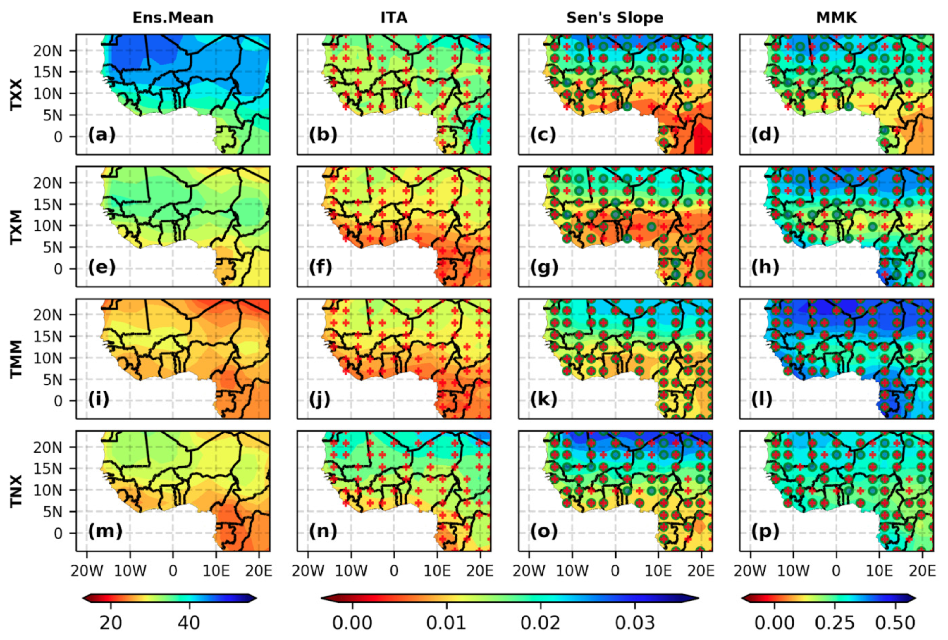
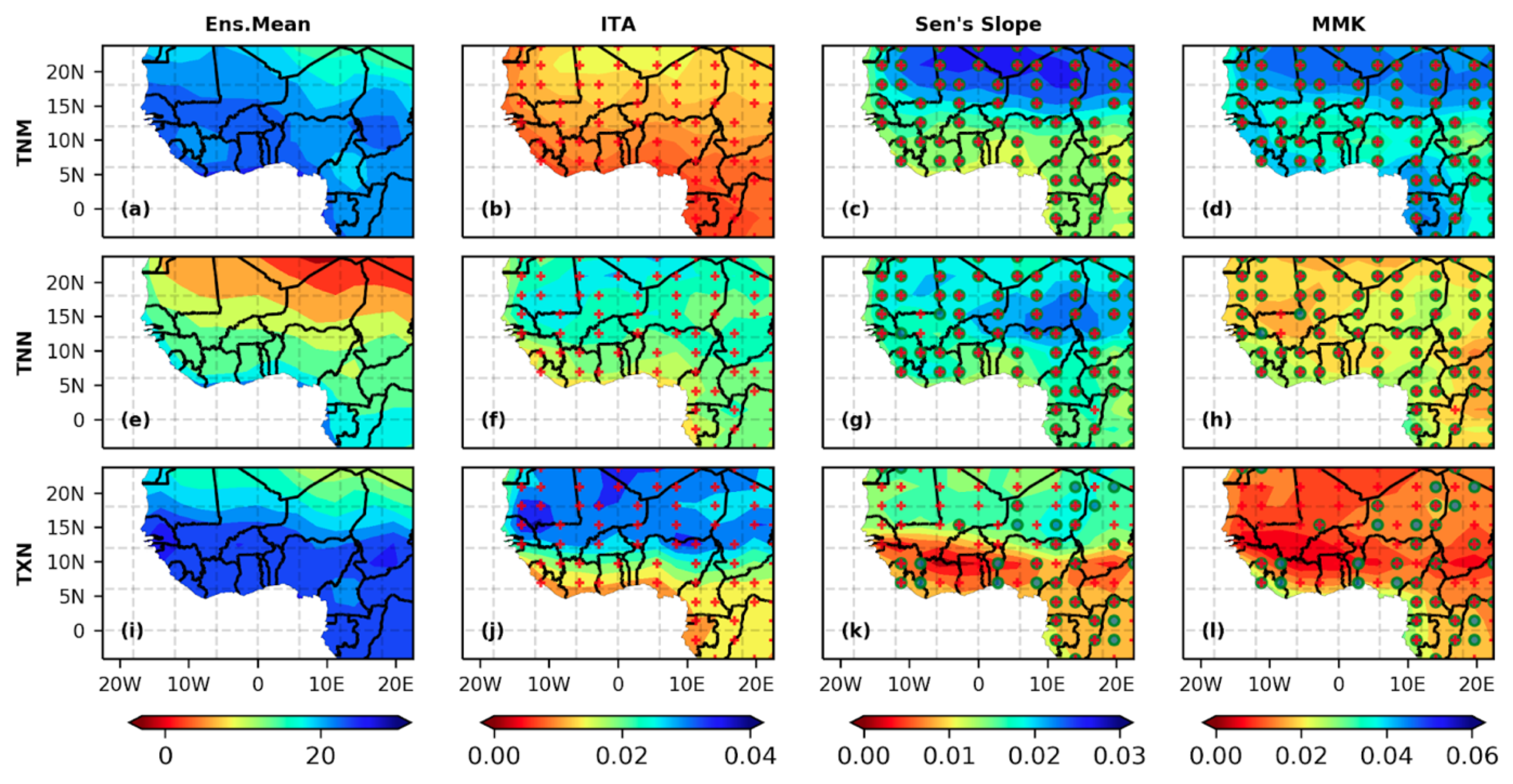
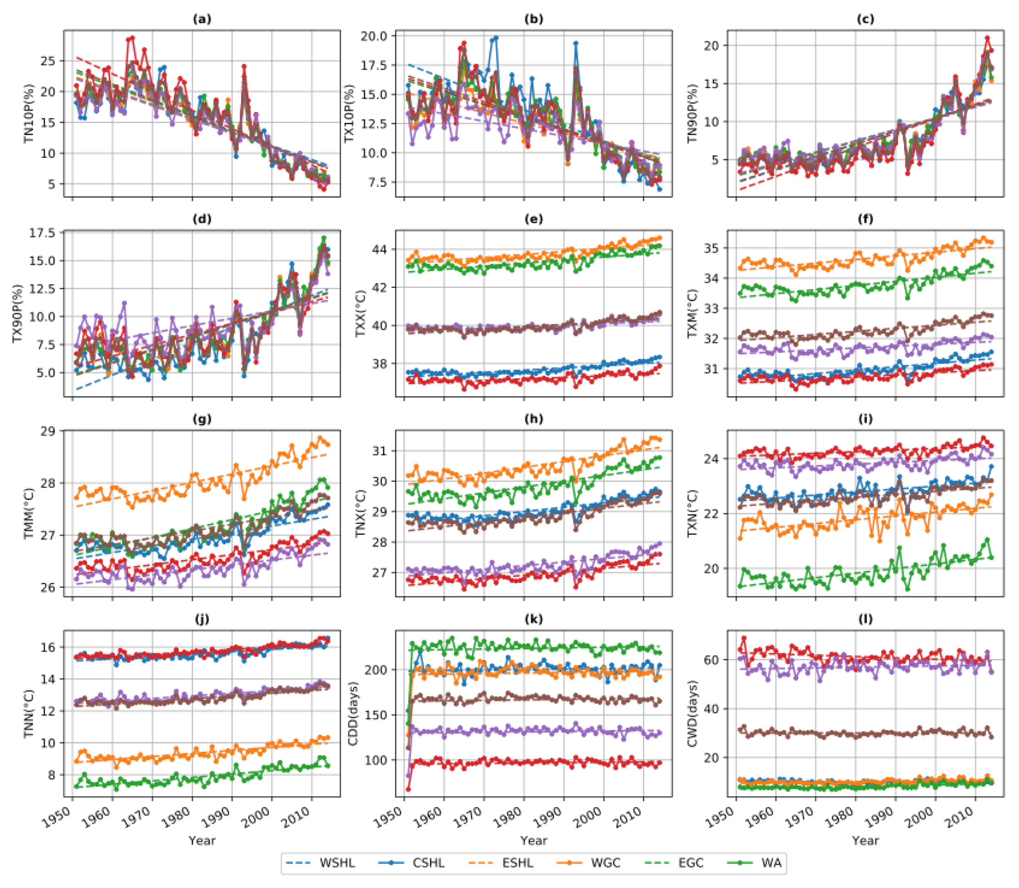
3.3.2. Absolute Extreme Temperature Indices (TXX, TXM, TMM, TNX, TNN, TNM, TXN)

Figure 11 presents the spatial average of the maximum values of daily maximum temperature (TXX), mean daily maximum temperature (TXM), mean daily mean temperature (TMM), and maximum value of daily minimum temperature (TNX). As analyzed previously for the maximum temperature trend, the maximum TXX was located in the northern part, and specifically the northwest (45 °C). The same went for TXM (43 °C), TMM, and TNX. The lowest maxima were located in the southern area. The analysis was based on the criterion that a minimum of 80% of models had to show the trend; thus, the red crosses (+) indicate that at least 80% of models agreed with the increasing trend (Figure 11). The green circles indicate where the trends were significant at 95% CL.

Regarding trends, all the statistical methods showed an increasing trend in maximum temperatures. The significant increase in maximum temperatures was higher in the north and lower in the south, with the appearance of a clear dynamic northward gradient. Sen’s slope test indicated an increase of about 0.1 to 0.3 °C/decade; the ITA method, 0.1 to 0.25 °C/decade; and the MMK method, a very high 0.2 to 0.5 °C/decade. The maximum of Tmax was located in the same area (northern part) under the three methods used, with increases of 0.15 °C/decade, 0.25 °C/decade, and 0.35 °C/decade under ITA, Sen’s, and MMK, respectively. The lowest value of the maximum of Tmax was across the GC. In contrast, the ITA overestimated the increasing trend of the maximum of Tmax over the Cameroon mountains and the Gabon forest compared to Sen’s and MMK. This representation of ITA was due to the fact that it brought out the small trend changes or trends over each year. The ratio of the maximum Tmax to the minimum Tmax (TXN) was 2.1 (Figure 12), which means that the maximum of Tmax was about 2.1 times greater than the minimum of Tmax, and this was almost verified under all three of the analysis methods adopted. The spatial average of Tmax, as well as the average of the mean temperature in Figure 12, expressed the same tendency of the increasing value from ITA to Sen’s to the MMK. In the southern regions, increasing trends were around 0.09 °C/decade, 0.07 °C/decade, and 0.2 °C/decade for the mean of Tmax and 0.09 °C/decade, 0.1 °C/decade, and 0.22 °C/decade for the mean of the spatial average temperature under the ITA, Sen’s, and MMK methods, respectively. The percentage of significant increase trend was 100% for an average mean temperature, greater than 70% for the maximum of the minimum temperature (TNx), and about 50% for the average of Tmax. Some areas were significantly increasing with 95% CL but were not shown by a minimum of 80% of models on which the authors agreed for the analysis in the present study.

3.4. Spatial Changes in Precipitation Indices

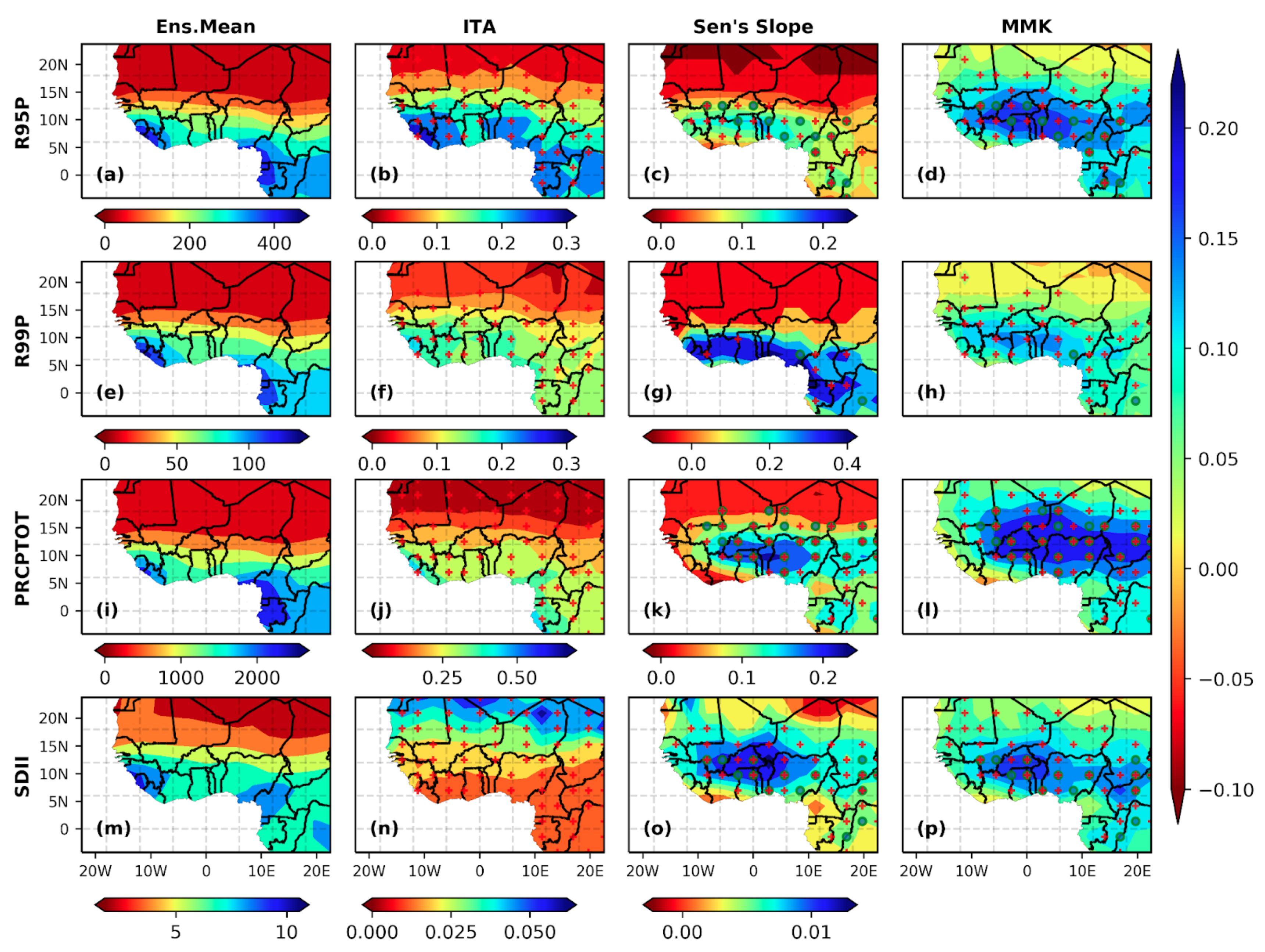
3.4.1. Percentile-Based Precipitation Indices (R95p, R99p)

The analysis of Figure 13 indicated that the R95p and R99p variabilities were regionally distributed, with the maximum in the south and the minimum in the north. The figure marks an increasing trend of the percentile of the two indices, with scatterings of significance (at least at 95% CL) in the south. Less than 80% of the models used indicated a change in the northern part of the study domain with Sen’s slope; it seems that the north did not have a clear change. However, both indices (R99p and R95p) recorded very low rainfall amounts (Figure 13a–h).

For both indices (R95p and R99p), the ITA and MMK methods faintly depicted an increasing trend in the north of 0.3 mm/decade and less than 0.4 mm/decade, respectively. All three methods attested to the existence of change in the southern area and confirmed the maxima located around the Guinea highlands, the Cameroon mountains, and the Gabon forests for both indices. The maximum of the total annual rainfall from the heavy rain days (R95p) was about 320 mm/year (located around Guinea, Cameroon, and Gabon); the maximum of the total annual rainfall from the very heavy rain days (R99p) was about 110 mm/year and was located at the same area as R95p. The increasing trend in the south for both indices was quietly important (from 2 to 4 mm/decade) but of scattered significance. The increasing trend in the heavy rain days was significant (at least 95% CL) over countries such as Gabon, Cameroon, the southern part of Nigeria, the northern part of Benin, Burkina Ghana, and the southern part of Mali. However, for R99p, the marked increasing trend was not significant in the south.

3.4.2. Absolute Extreme Precipitation Indices (RX1day, RX5day, RX7day)

The spatial display of the RX1day, RX5day, and RX7day varied widely and dynamically decreased from the south toward the north. From the data analysis, the average maximum RX1day of 65 mm was located between latitudes of 5° N and 12° N; that of RX5day, of about 121 mm, and that of RX7day, of about 169–187 mm, were located in the Guinea highlands, Cameroon, and Gabon.

The indices had a positive trend across the whole of WA, and the extrema of the changes converged with the extrema of the indices. The strict criteria well captured some scattered significant increasing trends (5% of the whole domain). Figure 14 indicates for the three indices a rise of 1 to 1.7 mm/decade, 1 to 2.5 mm/decade, and 1.5 to 3.7 mm/decade under MMK, Sen’s slope, and ITA, respectively, over the Savannah toward south. It was observed that the trends of these indices were quietly consistent but not significant everywhere. The more the number of cumulative days increased, the clearly southward the positive trend was oriented. In addition to the analysis of the R99p and R95p, this may impact the cumulative wet days in the southern region.

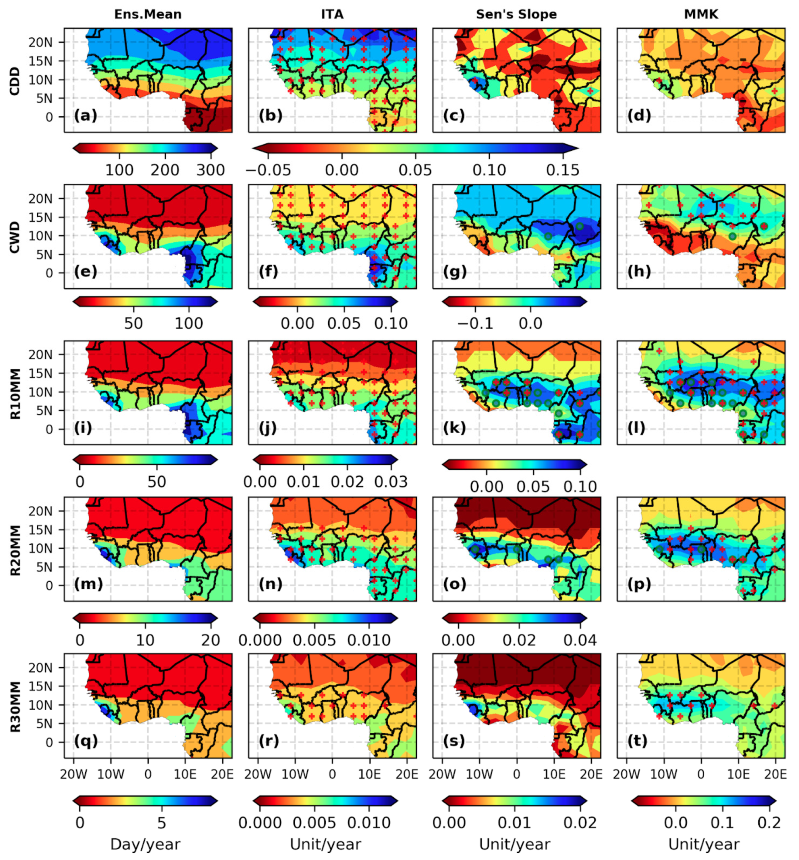
3.4.3. Threshold and Duration Extreme Precipitation Indices (R10mm, R20mm, R30mm, CDD, CWD)

Figure 15 illustrates the spatially averaged numbers of heavy rain days (R10mm), very heavy rain days (R20mm), extremely heavy rain days (R30mm), consecutive dry days (CDD), and consecutive wet days (CWD). They exhibited a slight, increasing southward trend, as in the case of R99p and R95p. The CDD was very high in the north (298 days/year) and low in the south (61 days/year). The CWD was high in the south (112 days/year in the Guinea Highlands and Cameroon–Gabon and 48–62 days/year in other areas) and low in the north (12 days/year). Regarding the change trends, Sen’s slope and MMK did not capture significant trends because of the high and strict criteria adopted in this study (the minimum of 80% of models that needed to express the trend). Focusing on the CDD, only a single decreasing trend was noticed, in the southeast of Niger, and an increase was observed in the southwest of the Congo. For the two analysis methods (Sen’s and MMK) applied to CDD, globally, the study domain experienced a nonsignificant decreasing trend, except for in the Guinea highlands, where an increase up to 1 day/decade was observed, and a scatter of some increasing trends over the northeastern and northwestern parts as well as countries such as Benin, Togo, Ghana, and Cote d’Ivoire. The analysis of ITA revealed a clear and dynamic distribution of trends, with an increase in the CDD in the northern regions (up to 1.3 days/decade) diminishing toward the south to 0.2 days/decade. The assessment of the CWD revealed, indirectly, a contrast with the CDD; the locations of CDD maxima coincided with the minima of CWD and vice versa. The MMK and Sen’s slope tests depicted, over the Guinea highlands and Cameroon, a decreasing trend in CWD. An increasing trend was noticed over the Savannah, and in the case of the MMK test, the change in some parts was captured based on the analysis criteria.

The R10mm, R20mm, and R30mm showed increasing trends over the whole of WA, with values of 0.12 to 0.2 day/decade, 0.04 to 0.1 day/decade, and 0.04 to 0.06 day/decade, respectively, over the Savannah and the south area under the ITA test. The Sen’s slope and MMK tests displayed the same trend dynamic, i.e., a southward increase in the number of days per decade. The increasing trend of the R10mm was significant in the southern regions, at about 1 day/decade under Sen’s slope and 2 days/decade under MMK. There was almost no trend of R10mm over the northern regions. The R20mm and the R30mm increased from the Savannah to the south. MMK and ITA, based on our criteria, captured the change, while Sen’s test could not. However, the Sen’s slope results depicted on average an augmentation of about 0.2 to 0.4 day/decade in the very heavy rain days in the southern part. In the case of R30mm, the observations were quite similar to those for the R20mm when applying Sen’s slope test. It was also noticed, based on the analysis criteria, that only the southern part of the WA experienced a nonsignificant increase trend, with picks around the Guinea highlands.

3.4.4. Other Indices (PRCPTOT and SDII)

The annual average of PRCPTOT (Figure 13) had a similar spatial distribution and trend to those of R95p and R99p, wherein the values of indices were higher in the southern regions (2000 mm/year around Guinea, Cameroon, and Gabon). Its positive southward trend was about 2 mm/decade (from Savannah to GC) for all the statistical tests analyzed. As the case of previous indices, ITA revealed a very slight trend in the northern area, as did Sen’s slope and MMK, of about 0.02 mm/decade.

The spatial distribution of the simple precipitation intensity indicator (SDII) presented in Figure 13, indicates a faithful correlation with PRCPTOT, as well as with R99p and R95p. The maxima and minima were located in corresponding areas from one index to another. SDII reached a maximum and minimum of 10 mm/day/year and less than 1 mm/day, respectively. According to the statistical methods and criteria applied in the present study, Sen’s slope and MMK indicated a high positive trend in the SDII over the Savannah of about 2 mm/day/decade and a lower positive trend in the northeast and southwest of Cote d’Ivoire of about 0.01 mm/day/decade (almost no trend). ITA also displayed a positive trend in the SDII, but in contrast with the results obtained under MMK and Sen’s slope, the maximum of the increase lay in the northern regions, with an increase up to 0.5 mm/day/decade. The trend in the central part of WA rose to 0.25 mm/day/decade.

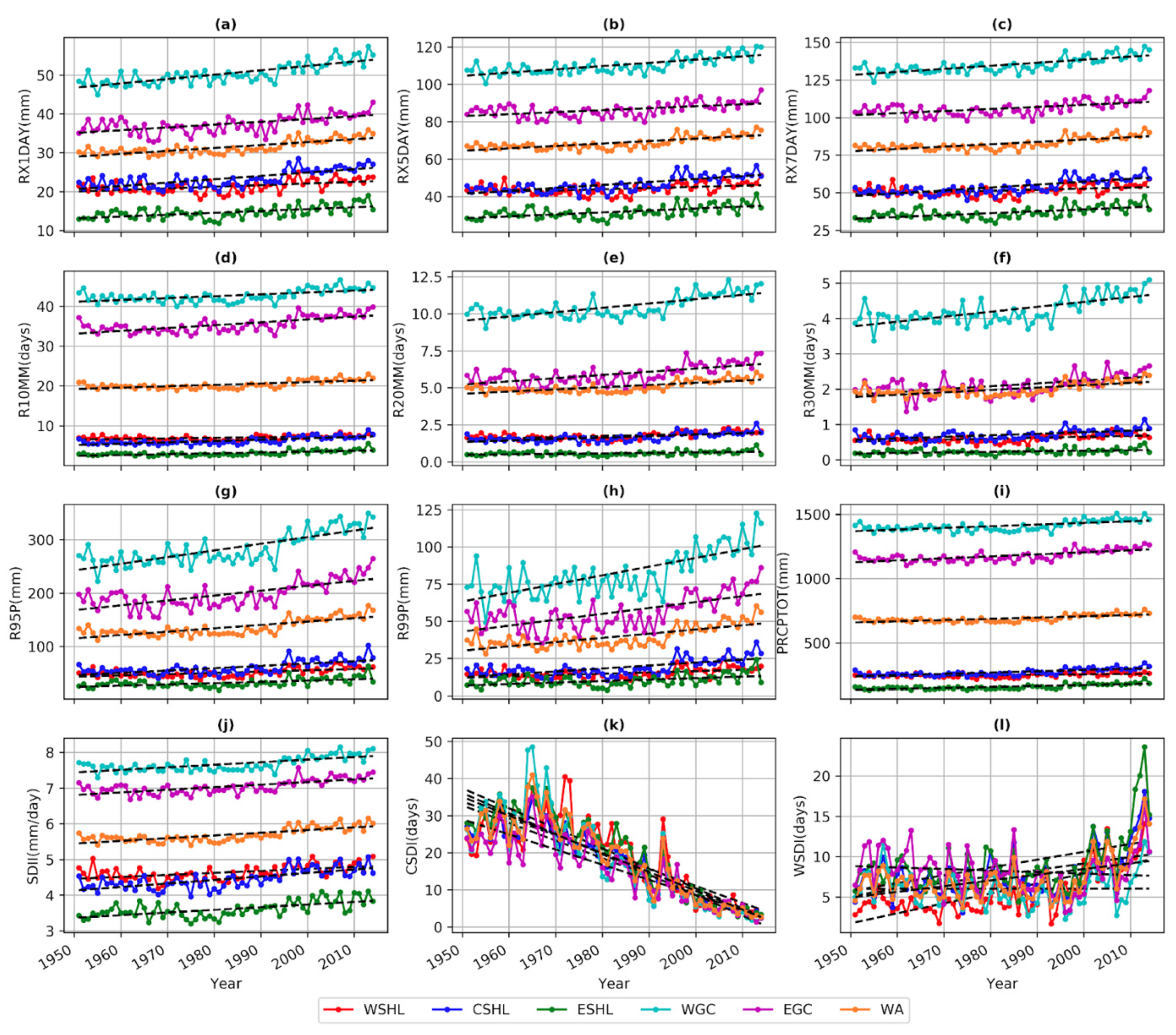
3.5. Temporal Variability of Precipitation and Temperatures Indices

In this part, for better evaluation of the temporal variabilities [91], temporal analysis of trends was performed over five subregions [92] (West Sahel: WSHL, Central Sahel: CSHL, East Sahel: ESHL, West Guinea Coast: WGC, and East Guinea Coast: EGC) and the whole study domain (West Africa: WA).The cold indices TX10p, TN10p (Figure 16a,b), and CSDI (Figure 17k) globally expressed a temporal negative trend. The change trends were almost identical for the five subregions and the whole domain.

A slight upward trend of about +0.05 day/decade was revealed from 1950 to 1962, when the largest value is recorded, followed by a consistent detrend of about −0.35 day/decade from 1963 to 2014, with a spike (break) in 1992. However, the warm indices TX90p and TN90p (Figure 16c,d), as well as WSDI (Figure 17l), displayed two major trends, a slight upward trend (0.01 day/decade) in 1950–1992 (1950–2000) for TX90p and TN90p (WSDI), and the positive trend became more important (0.46 day/decade) in 1993–2013 (2001–2014) for TX90p and TN90p (WSDI), up to an average maximum value of 16 days and 19 days (16 days) a year, respectively. For WSDI, the ESHL increased greatly from 2010 to 2012 and seemed to exhibit the same increase as in the case of TX90p, while over WGC, the TN90p, which recorded smaller values since 1950, rose up starting in 2000 to reach its peak in 2013. The above analysis indicated that nighttime cooling was higher than daytime cooling in the period 1993–2014, and over the same period, it was observed that nighttime warming was higher than daytime warming.

Figure 17 depicts the overall upward trend for indices including RX1day, RX5day, RX7day, R10mm, R20mm, and R30mm, as well as R99p, R95p, and PRCPTOT. All the indices showed both upward and downward trends (not clear trends) from 1950–1992. However, from 1993–2014, they slightly increased. For these indices, the WGC received the maximum rainfall amount, followed by the EGC and the whole domain. Very large differences between values were noted from one subregion to another. Obviously, the values of WSHL and CSHL were close, since they are located at the same latitude. This confirms that the rainfall experience over West Africa was due to the swaying of the West African Monsoon (WAM). The temporal representation of the change in CDD is opposite to that of the change in CWD for each subregion. There was an increase in CWD over WSHL, CSHL, and ESHL and a slight decrease over WGC and EGC, but the trends were mixed over the whole period. The overall trend (WA) was upward, with +0.012 day/decade. For the subregions, there was no obvious trend in CDD. However, the highest value of CDD was registered over the ESHL and seemed to then decrease from 1992–2014 by 0.009 day/decade. The CSHL trends were alternatively upward and downward in 1950–2014, while the upward and download trends over WSHL led to an overall increase of about +0.024 day/decade. The lowest values of CDD were located in WGC, which showed a decreasing trend in CDD over the whole region. On the other side, the lowest CWD was closed, located over WSHL, CSHL, and ESHL, and overall followed an upward trend of about 0.021 day/decade. The highest CWD (about 59 ± 6) was located in subregions such as WGC and EGC but showed a decreasing trend over time.

Figure 16 presents the absolute indices, i.e., maximum of Tmax (TXX), mean of Tmax (TXM), the average of the mean temperature (TMM), the maximum of Tmin (TNX), the minimum of Tmax (TXN), and the minimum of Tmin (TNN), and indicates a positive trend for each of them over the 65 years (1950–2014). The change in the cited indices was overall parallel from a region to another, and a break in the trend in 1992 could be noted for all of them. TXX rose by 0.02 °C/decade from 1950–1992, and from 1993–2014, the upward change was about 0.07 °C/decade. TXM, TXN, and TNX positively changed by about 0.01 °C/decade from 1950–1992 but from 1993–2014 increased at rates of about 0.06 °C/decade, 0.01 °C/decade, and 0.059 °C/decade, respectively.

4. Discussion

Some recent studies [46,47,93] investigated the performance of CMIP6 models and found that they had a better performance in regard to precipitation than CMIP5 models. In the present research, the spatial and temporal evolution of extreme climate events over the whole of West Africa and its five subregions during the period 1950–2014 was analyzed based on the CMIP6 dataset by selecting some indices of extreme temperature and precipitation.

The precipitation over WA was widely distributed when considering individual models. As aforementioned, monsoon period rain contributes more than 85% of the total annual precipitation over the latitudes 5° N–20° N. This seems to agree with [94], which found that in September, the rainfall was the highest (about 30.85% contribution of the total annual amount) and slightly increased from August (29.44%). The present study illustrated that the area with a decrease in total annual rainfall, as revealed by the models, was the Guinea Highlands, while Cameroon, Gabon, and the Savannah exhibited the highest increasing trends (Figure 5). Regarding the extreme precipitation in WA, the study depicted strong links of its changes to climatic zones and showed its increase over the study period in Savannah. The identification and location of the trends were the same under all the statistical methodologies applied; the trends differed only in their magnitudes. The trends in precipitation were enhanced with the results on percentile-based metrics, which revealed the existence of a gradual north–south trend. The result converged with [95], which noted a drying trend over WA from 1951 to 2012. Additionally, ref. [96] noticed that during the period 1990–2010, both annual rainfall and the frequency of rainy days increased, leading to partial recovery from the severe dry period recorded in WA in the 1970s. This dryness was studied in [97,98], wherein it was illustrated that at the beginning of the 1970s, all climatic zones in tropical West Africa, from the arid Sahelian to the humid Guinea Coast climate, experienced a decade-long period of below-normal annual rainfall amounts. This finding converged with analysis of the temporal variability of trend, which revealed the existence of a breakpoint in 1992. Ref. [97] noted a decrease in the number of rainy events over the central Sahelian country of Niger in the two dry decades from 1970 to 1989; the results showed a quasinormal condition (or a slight increase) for temperature and precipitation from 1950–1992. A study led by [99] associated the “recovery” of WA in the 1990s to greenhouse gas (GHG) changes noticed between 1910 and 2008. This recovery in rainfall will influence the climate water balance (CWB, refs. [20,24]) and increase uncertainty in regard to hydrology, agriculture, and climate change. Although a general downward trend was noticed in the north, the ITA and MMK tests captured the existence of slight increases in R95p and R99p within the region and confirmed the maximum location as well as an upward trend in the amount of rainfall received around the Guinea highlands, Cameroon mounts, and Gabon forests. These results agreed with previous studies [47,100], which identified similar trends. Additionally, the present study indicated that the more the number of cumulative days increased, the more important the positive trend in the amount of rainfall received in the south was. R95p illustrated a significant positive trend in heavy rainfall near countries such as Gabon, Cameroon, the southern part of Nigeria, the northern part of Benin, Burkina Ghana, and the southern part of Mali. According to [101], it was expected that the number of consecutive dry days would be more pronounced in the northern regions than in the southern. The same analysis led to the conclusion in [102] that rainfall in the littoral zone of southern WA was more extreme than that inland.

The temperature has, over most regions across the world, an increasing trend. The annual means of daily maximum and minimum temperature exhibited a significant increase during the focus study period (1950–2014). Ref. [103] discovered the same warming trends over WA, while [104,105] found similar results in Eastern and Southern Africa, respectively. Ref. [106] reported that the temperature increase in high latitudes was greater than that in low latitudes. Regarding the temperature extreme changes in the whole of WA, TN90, TX90p, and WSDI indicated a general warming trend. That result was in line with the findings in [107] during the period 1979–2005, where an upward trend was noted in TX90p and TN90p associated with an increase in WDSI. The cold nights (days), TN10p (TX10p), showed a southward declining trend. This observation was confirmed by [101], which identified uniform declining trends in TN10p and TX10p over WA. Furthermore, during the period 1950–2014, the trends of cool/warm nights (TN10p/TX90p) were more significant than those of cool/warm days (TX10p/TX90p); this justifies the finding of [56], which reached the same conclusion over China. The absolute extreme temperature indices, such as TXX, TXM, TMM, TNX, TNN, TNM, and TXN, experienced an increasing trend over the whole study area. The Sahel area became warmer, with significantly high values noticed; a clear northward dynamic gradient was well represented. Overall, clear warming weather events were experienced in WA, with significant increases in all the extreme temperatures. This change in climate conditions revealed the manifest effect of climate change in the study domain. Studying the temporal variability and trends of temperature, the study revealed that the cold indices TX10p, TN10p (Figure 16a,b), and CSDI (Figure 17k) expressed a general temporal negative trend. Those indices had breakpoints within their trends in 1962 in terms of temperature change because, prior to the clear declining trend, the indices observed a slight increase from 1950 to 1962 before adopting an upward trend until the end of the study period (2014).

The present study revealed that in WA, very few positive trends of CDD were generally observed, with the maxima converging in the northern part as well as over some other countries (Benin, Togo, Ghana, and Cote d’Ivoire). However, the increasing trends of CDD reduced southwardly. A contrast was noticed in that the area receiving a lot of rainfall (Guinea Highlands, Cameroon mounts, and Gabon forests) displayed a decreasing trend in CWD, while the savannah was more wet. The trends regarding CDD and CWD confirmed findings from [103]. The negative trend in CWD was directly correlated with a southward increase of R10mm, R20mm, and R30mm in WA, similarly as in the findings in [20], which detected increasing R10mm and R20mm over the orographic regions and the ocean boundary (Gulf of Guinea). Changes in CDD and CWD can lead to uneven temporal distributions of rainfall. It is manifest that the persistence in the upward trend in CDD and the simultaneous downward trend in CWD led to a negative impact on the PRCPTOT trend over the study domain and could have a negative influence on the water resource demand in WA in general and especially in the northern regions. This may lead to efforts to further irrigation plans to supply the needs of water for agriculture production in the northern area. Furthermore, the southward diminution in CWD might induce a reduction in the number of times WA is watered, and the concurrent upward noticed in SDII and the R30mm might induce localized floodlike situations over the southern regions. It is important to note that CDD and CWD are crucial in the magnitude of flooding (especially flash flooding) events because of their implications on the soil moisture state before the occurrence of flooding. Moreover, as [108] indicated, increasing soil moisture reduces the infiltration capacity of the study domain and then fosters flooding occurrence. A very strong correlation was noticed among R99p, R95p, and PRCPTOT. The increase in PRCPTOT over WA was illustrated in previous studies [103,107]. This attests that other rainfall events over the area did not contribute much to the total annual rainfall amount. Indirectly, extreme rainfall events increased in intensity in the southern area and might be the most accountable for the total annual rainfall.

5. Conclusions

In this study, the long-term spatial and temporal variabilities of and changes in rainfall and temperature were analyzed. Based on climate indices suggested by ETCCDMI, the study applied three statistical tests to assess the trends in the two variables. The following conclusions from the study can be made:

• The total annual rainfall was found to decrease around the coastal area, especially over the Guinea highlands, the Cameroon mountains, as the Gabon forests, but increase over the Savannah and Sahel regions. Furthermore, rainfall during the monsoon months contributed more than 85% of the total annual rainfall in the study domain.
• The interannual Tmax and Tmin both followed the same trends as the total annual rainfall, with a northward gradient. The warmest region was the Savannah–Sahel, while the coastal part was the coolest area. Using ITA, particular increasing trends were identified from the models in the northern part and the Guinea coast. The increasing trends around the Guinea coast may be due to the gradual increase in sea surface temperature (SST) due to global warming (GW).
• Extreme high-temperature indices (warm extremes) significantly increased, while the cold extremes indicated a significant upward trend. Both indices showed a breakpoint (abrupt changing point) in 1992, after which the trend increased more in power.
• The study revealed that the more the number of cumulative days increases, the more important the positive trend in the amount of rainfall received in the south was. Based on analysis of indices such as TN90, TX90p, and WSDI, the study also indicated a general warming trend over the whole of WA. However, over the study period, the trends in cool/warm nights (TN10p/TX90p) are more significant than those in cool/warm days (TX10p/TX90p).
• The upward trend in CDD and simultaneous downward trend in CWD led to a negative impact on the PRCPTOT trend over WA. This may affect water resource demand in general in WA and especially in the northern areas. Moreover, the decline in CWD showed a reduction in the wet spells in WA, and the concurrent upward notice in SDII and the R30mm might induce localized floodlike situations over the southern regions. Thus, it is important to note that CDD and CWD are crucial in regard to the magnitude of flooding events because of their implications on the soil moisture state before the occurrence of floods.
• The innovative trend analysis (ITA) methodology applied in this work was able to capture the most minute trends existing in a time series, including some that could not be detected by the usual tests so far used, such as Mann–Kendall and Sen’s slope. The reliability of ITA in tracking unseen trends in time-series data encourages us to recommend it to the reader as a reliable method to be used in time-series trend detection.
• Information gathered together from this study can contribute to producing sustainable water resource planning and management. It could also be useful for policy makers and scientists for exploring extreme climate event trends on regional and local scales to plan the circumstances in which potential floods and droughts might occur.

References

1. Peterson, T.; Manton, M. Monitoring Changes in Climate Extremes: A Tale of International Collaboration. Bull. Am. Meteorol. Soc. 2008, 89, 1266–1271. [Google Scholar] [CrossRef]
2. Tierney, J.E.; Smerdon, J.E.; Anchukaitis, K.J.; Seager, R. Multidecadal variability in East African hydroclimate controlled by the Indian Ocean. Nature 2013, 493, 389–392. [Google Scholar] [CrossRef] [Green Version]
3. Morice, C.P.; Kennedy, J.J.; Rayner, N.A.; Jones, P.D. Quantifying uncertainties in global and regional temperature change using an ensemble of observational estimates: The HadCRUT4 data set. J. Geophys. Res. 2012, 117, D08101. [Google Scholar] [CrossRef]
4. McCarthy, M.P.; Best, M.J.; Betts, R.A. Climate change in cities due to global warming and urban effects. Geophys. Res. Lett. 2010, 37. [Google Scholar] [CrossRef] [Green Version]
5. York, R.; Rosa, E.A.; Dietz, T. A rift in modernity? assessing the anthropogenic sources of global climate change with the STIRPAT model. Int. J. Sociol. Soc. Policy 2003, 23, 31–51. [Google Scholar] [CrossRef]
6. Gebrechorkos, S.H.; Hülsmann, S.; Bernhofer, C. Changes in temperature and precipitation extremes in Ethiopia, Kenya, and Tanzania. Int. J. Climatol. 2019, 39, 18–30. [Google Scholar] [CrossRef] [Green Version]
7. Sutton, M.A.; van Grinsven, H.; Billen, G.; Bleeker, A.; Bouwman, A.F.; Oenema, O. European Nitrogen Assessment—Summary for policymakers. In the European Nitrogen Assessment. Sources, Effects and Policy Perspectives; Sutton, M.A., Howard, C.M., Erisman, J.W., Billen, G., Bleeker, A., Grennfelt, P., van Grinsven, H., Grizzetti, B., Eds.; Cambridge University Press: Cambridge, UK, 2011. [Google Scholar] [CrossRef]
8. Barros, V.R.; Field, C.B.; Dokken, D.J.; Mastrandrea, M.D.; Mach, K.J.; Bilir, T.E.; Chatterjee, M.; Ebi, K.L.; Estrada, Y.O.; Genova, R.C.; et al. IPCC, Climate Change 2014: Impacts, Adaptation, and Vulnerability. Part B: Regional Aspects. In Contribution of Working Group II to the Fifth Assessment Report of the Intergovernmental Panel on Climate Change; Cambridge University Press: Cambridge, UK; New York, NY, USA, 2014; p. 688. [Google Scholar] [CrossRef] [Green Version]
9. Collins, J.M. Temperature variability over Africa. J. Clim. 2011, 24, 3649–3666. [Google Scholar] [CrossRef] [Green Version]
10. Barkhordarian, A.; von Storch, H.; Behrangi, A.; Loikith, P.C.; Mechoso, C.R.; Detzer, J. Simultaneous regional detection of land-use changes and elevated GHG levels: The case of spring precipitation in tropical South America. Geophys. Res. Lett. 2018, 45, 6262–6271. [Google Scholar] [CrossRef] [Green Version]
11. Bucchignani, E.; Mercogliano, P.; Panitz, H.J.; Montesarchio, M. Climate change projections for the Middle East-North Africa domain with COSMO-CLM at different spatial resolutions. Adv. Clim. Chang. Res. 2018, 9, 66–80. [Google Scholar] [CrossRef]
12. Lelieveld, J.; Hadjinicolaou, P.; Kostopoulou, E.; Chenoweth, J.; El Maayar, M.; Giannakopoulos, C.; Giannakopoulos, C.; Hannides, C.; Lange, M.A.; Tanarhte, M.; et al. Climate change and impacts in the Eastern Mediterranean and the Middle East. Clim. Chang. 2012, 114, 667–687. [Google Scholar] [CrossRef] [Green Version]
13. Lelieveld, J.; Proestos, Y.; Hadjinicolaou, P.; Tanarhte, M.; Tyrlis, E.; Zittis, G. Strongly increasing heat extremes in the Middle East and North Africa (MENA) in the 21st century. Clim. Chang. 2016, 137, 245–260. [Google Scholar] [CrossRef] [Green Version]
14. Almazroui, M.; Saeed, S.; Islam, M.N.; Khalid, M.S.; Alkhalaf, A.K.; Dambul, R. Assessment of uncertainties in projected temperature and precipitation over the Arabian Peninsula: A comparison between different categories of CMIP3 models. Earth Syst. Environ. 2017, 1, 1–21. [Google Scholar] [CrossRef]
15. Almazroui, M.; Islam, M.N.; Saeed, S.; Alkhalaf, A.K.; Dambul, R. Assessment of uncertainties in projected temperature and precipitation over the Arabian Peninsula using three categories of Cmip5 multimodel ensembles. Earth Syst. Environ. 2017, 1, 1–20. [Google Scholar] [CrossRef] [Green Version]
16. IPCC. Climate Change 2014: Synthesis Report. Contribution of Working Groups I, II and III to the Fifth Assessment Report of the Intergovernmental Panel on Climate Change; Core Writing Team, Pachauri, R.K., Meyer, L.A., Eds.; IPCC: Geneva, Switzerland, 2014; p. 151. [Google Scholar]
17. Chou, C.; Lan, C. Changes in the Annual Range of Precipitation under Global Warming. J. Clim. 2011, 25, 222–235. [Google Scholar] [CrossRef] [Green Version]
18. Gao, Y.; Cuo, L.; Zhang, Y. Changes in Moisture Flux over the Tibetan Plateau during 1979–2011 and Possible Mechanisms. J. Clim. 2014, 27, 1876–1893. [Google Scholar] [CrossRef]
19. Quenum, G.M.L.D.; Klutse, N.A.; Dieng, D.; Laux, P.; Arnault, J.; Kodja, J.D.; Oguntunde, P.G. Identification of potential drought areas in West Africa under climate change and variability. Earth Syst. Environ. 2019, 3, 429–444. [Google Scholar] [CrossRef] [Green Version]
20. Quenum, G.M.L.D.; Klutse, N.A.; Alamou, E.A.; Lawin, E.A.; Oguntunde, P.G. Precipitation Variability in West Africa in the Context of Global Warming and Adaptation Recommendations. In African Handbook of Climate Change Adaptation; Leal Filho, W., Oguge, N., Ayal, D., Adeleke, L., da Silva, I., Eds.; Springer: Berlin/Heidelberg, Germany, 2020; pp. 1–22. [Google Scholar] [CrossRef]
21. Van Vuuren, D.P.; Edmonds, J.; Kainuma, M.; Riahi, K.; Thomson, A.; Hibbard, K.; George, C.H.; Kram, T.; Krey, V.; Lamarque, J.F.; et al. The representative concentration pathways: An overview. Clim. Chang. 2011, 109, 5. [Google Scholar] [CrossRef]
22. Sawadogo, W.; Abiodun, B.J.; Okogbue, E.C. Projected changes in wind energy potential over West Africa under the global warming of 1.5 °C and above. Theor. Appl. Climatol. 2019, 138, 321–333. [Google Scholar] [CrossRef]
23. Kumi, N.; Abiodun, B.J. Potential impacts of 1.5 C and 2 C global warming on rainfall onset, cessation and length of rainy season in West Africa. Environ. Res. Lett. 2018, 13, 055009. [Google Scholar] [CrossRef]
24. Abiodun, B.J.; Makhanya, N.; Petja, B.; Abatan, A.A.; Oguntunde, P.G. Future projection of droughts over major river basins in Southern Africa at specific global warming levels. Theor. Appl. Climatol. 2019, 137, 1785–1799. [Google Scholar] [CrossRef]
25. Klutse, N.A.B.; Ajayi, V.O.; Gbobaniyi, E.O.; Egbebiyi, T.S.; Kouadio, K.; Nkrumah, F.; Quagraine, K.A.; Olusegun, C.; Diasso, U.; Dosio, A.; et al. Potential impact of 1.5 C and 2 C global warming on consecutive dry and wet days over West Africa. Environ. Res. Lett. 2018, 13, 055013. [Google Scholar] [CrossRef]
26. Maúre, G.; Pinto, I.; Ndebele-Murisa, M.; Muthige, M.; Lennard, C.; Nikulin, G.; Dosio, A.; Meque, A. The southern African climate under 1.5 C and 2 C of global warming as simulated by CORDEX regional climate models. Environ. Res. Lett. 2018, 13, 065002. [Google Scholar] [CrossRef]
27. Nikulin, G.; Lennard, C.; Dosio, A.; Kjellström, E.; Chen, Y.; Hänsler, A.; Kupiainen, M.; Laprise, R.; Mariotti, L.; Somot, S.; et al. The effects of 1.5 and 2 degrees of global warming on Africa in the CORDEX ensemble. Environ. Res. Lett. 2018, 13, 065003. [Google Scholar] [CrossRef]
28. Nguyen, T.H.; Min, S.K.; Paik, S.; Lee, D. Time of emergence in regional precipitation changes: An updated assessment using the CMIP5 multi-model ensemble. Clim. Dyn. 2018, 51, 3179–3193. [Google Scholar] [CrossRef]
29. Nikiema, P.M.; Sylla, M.B.; Ogunjobi, K.; Kebe, I.; Gibba, P.; Giorgi, F. Multi-model CMIP5 and CORDEX simulations of historical summer temperature and precipitation variabilities over West Africa. Int. J. Climatol. 2017, 37, 2438–2450. [Google Scholar] [CrossRef]
30. Almazroui, M.; Şen, Z.; Mohorji, A.M.; Islam, M.N. Impacts of climate change on water engineering structures in arid regions: Case studies in Turkey and Saudi Arabia. Earth Syst. Environ. 2019, 3, 43–57. [Google Scholar] [CrossRef]
31. De Longueville, F.; Ozer, P.; Gemenne, F.; Henry, S.; Mertz, O.; Nielsen, J.Ø. Comparing climate change perceptions and meteorological data in rural West Africa to improve the understanding of household decisions to migrate. Clim. Chang. 2020, 160, 123–141. [Google Scholar] [CrossRef]
32. Nicholson, S.E.; Ba, M.B.; Kim, J.Y. Rainfall in the Sahel during 1994. J. Clim. 1996, 9, 1673–1676. [Google Scholar] [CrossRef] [Green Version]
33. Hulme, M.; Doherty, R.; Ngara, T.; New, M.; Lister, D. African climate change: 1900–2100. Clim. Res. 2001, 17, 145–168. [Google Scholar] [CrossRef] [Green Version]
34. Nicholson, S.E. On the question of the “recovery” of the rains in the West African Sahel. J. Arid. Environ. 2005, 63, 615–641. [Google Scholar] [CrossRef]
35. van de Giesen, N.; Liebe, J.; Jung, G. Adapting to climate change in the Volta Basin. West Afr. Curr. Sci. 2010, 98, 1033–1038. [Google Scholar]
36. Mounir, Z.M.; Ma, C.M.; Amadou, I. Application of Water Evaluation and Planning (WEAP): A model to assess future water demands in the Niger River (in Niger Republic). Mod. Appl. Sci. 2011, 5, 38–49. [Google Scholar] [CrossRef] [Green Version]
37. Gray, C.; Wise, E. Country-specific effects of climate variability on human migration. Clim. Chang. 2016, 135, 555–568. [Google Scholar] [CrossRef] [PubMed] [Green Version]
38. Henry, S.; Piché, V.; Ouédraogo, D.; Lambin, E.F. Descriptive analysis of the individual migratory pathways according to environmental typologies. Popul. Environ. 2004, 25, 397–422. [Google Scholar] [CrossRef]
39. FAO. The State of Agricultural Commodity Markets 2015–2016. In Trade and Food Security: Achieving a Better Balance between National Priorities and the Collective Good; Food and Agriculture Organization of the United Nations: Rome, Italy, 2015; Available online: http://www.fao.org/publications/soco/the-state-of-agricultural-commodity-markets-2015-16/en/ (accessed on 19 April 2018).
40. Halimatou, A.T.; Kalifa, T.; Kyei-Baffour, N. Assessment of changing trends of daily precipitation and temperature extremes in Bamako and Ségou in Mali from 1961–2014. Weather Clim. Extrem. 2017, 18, 8–16. [Google Scholar] [CrossRef]
41. Ogilvie, A.; Mahe, G.; Ward, J.; Serpantie, G.; Lemoalle, J.; Morand, P.; Barbier, B.; Diop, A.T.; Caron, A.; Namarra, R.; et al. Water, agriculture and poverty in the Niger River Basin. Water Int. 2010, 5, 594–622. [Google Scholar] [CrossRef]
42. Patricola, C.M.; Cook, K.H. Sub-Saharan Northern African climate at the end of the twenty-first century: Forcing factors and climate change processes. Clim. Dyn. 2011, 37, 1165–1188. [Google Scholar] [CrossRef] [Green Version]
43. Szwed, M.; Karg, G.; Pinskwar, I.; Radziejewski, M.; Graczyk, D.; Kedziora, A.; Kundzewicz, Z.W. Climate change and its effect on agriculture, water resources and human health sectors in Poland. Nat. Hazards Earth Syst. Sci. 2010, 10, 1725–1737. [Google Scholar] [CrossRef]
44. Oguntunde, P.G.; Abiodun, B.J. The impact of climate change on the Niger River Basin hydroclimatology. West Afr. Clim. Dyn. 2013, 40, 81–94. [Google Scholar] [CrossRef]
45. Osuch, M.; Romanowicz, R.J.; Lawrence, D.; Wong, W.K. Assessment of the influence of bias correction on meteorological drought projections for Poland. Hydrol. Earth Syst. Sci. Discuss. 2015, 12, 10331–10377. [Google Scholar]
46. Almazroui, M.; Saeed, F.; Saeed, S.; Islam, M.N.; Ismail, M.; Klutse, N.A.B.; Siddiqui, M.H. Projected change in temperature and precipitation over Africa from CMIP6. Earth Syst. Environ. 2020, 4, 455–475. [Google Scholar] [CrossRef]
47. Klutse, N.A.B.; Quagraine, K.A.; Nkrumah, F.; Quagraine, K.T.; Berkoh-Oforiwaa, R.; Dzrobi, J.F.; Sylla, M.B. The climatic analysis of summer monsoon extreme precipitation events over West Africa in CMIP6 simulations. Earth Syst. Environ. 2021, 5, 25–41. [Google Scholar] [CrossRef]
48. Cooper, P.J.M.; Dimes, J.; Rao, K.P.C.; Shapiro, B.; Shiferaw, B.; Twomlow, S. Coping better with current climatic variability in the rain-fed farming systems of sub-Saharan Africa: An essential first step in adapting to future climate change? Agric. Ecosyst. Environ. 2008, 126, 24–35. [Google Scholar] [CrossRef] [Green Version]
49. Sultan, B.; Gaetani, M. Agriculture in West Africa in the Twenty-First Century: Climate Change and Impacts Scenarios, and Potential for Adaptation. Front. Plant Sci. 2016, 7, 1262. [Google Scholar] [CrossRef] [Green Version]
50. Esham, M.; Garforth, C. Agricultural adaptation to climate change: Insights from a farming community in Sri Lanka. Mitig. Adapt. Strateg. Glob. Chang. 2013, 18, 535–549. [Google Scholar] [CrossRef]
51. Crimp, S.J.; Stokes, C.J.; Howden, S.M.; Moore, A.D.; Jacobs, B.; Brown, P.R.; Leith, P. Managing Murray–Darling Basin livestock systems in a variable and changing climate: Challenges and opportunities. Rangel. J. 2010, 32, 293–304. [Google Scholar] [CrossRef]
52. Rosenzweig, C.; Jones, J.W.; Hatfield, J.L.; Ruane, A.C.; Boote, K.J.; Thorburn, P.; Antle, J.M.; Nelson, G.S.; Porter, C.; Asseng, S.; et al. The agricultural model intercomparison and improvement project (AgMIP): Protocols and pilot studies. Agric. For. Meteorol. 2013, 170, 166–182. [Google Scholar] [CrossRef] [Green Version]
53. Faye, A.; Akinsanola, A.A. Evaluation of extreme precipitation indices over West Africa in CMIP6 models. Clim. Dyn. 2021, 1–15. [Google Scholar] [CrossRef]
54. Diasso, U.; Abiodun, B.J. Drought modes in West Africa and how well CORDEX RCMs simulate them. Theor. Appl. Climatol. 2017, 128, 223–240. [Google Scholar] [CrossRef]
55. Funk, C.; Peterson, P.; Peterson, S.; Shukla, S.; Davenport, F.; Michaelsen, J.; Knapp, K.R.; Landsfeld, M.; Husak, G.; Harrison, L.; et al. A high-resolution 1983–2016 Tmax climate data record based on infrared temperatures and stations by the Climate Hazard Center. J. Clim. 2019, 32, 5639–5658. [Google Scholar] [CrossRef]
56. Frich, P.; Alexander, L.V.; Della-Marta, P.; Gleason, B.; Haylock, M.; Tank, A.M.G.K.; Peterson, T. Observed coherent changes in climatic extremes during the second half of the twentieth century. Clim. Res. 2002, 19, 193–212. [Google Scholar] [CrossRef] [Green Version]
57. Zhang, X.; Alexander, L.; Hegerl, G.C.; Jones, P.; Tank, A.K.; Peterson, T.C.; Trewin, B.; Zwiers, F.W. Indices for monitoring changes in extremes based on daily temperature and precipitation data. Wiley Interdiscip. Rev. Clim. Chang. 2011, 2, 851–870. [Google Scholar] [CrossRef]
58. Mann, H.B. Nonparametric tests against trend. Econometrica 1945, 13, 245–259. [Google Scholar] [CrossRef]
59. Kendall, M.G. Rank Correlation Methods; Charles Griffin: London, UK, 1975; p. 1955. [Google Scholar]
60. Sen, P.K. Estimate of the regression coefficient based on Kendall’s tau. J. Am. Stat. Assoc. 1968, 63, 1379–1389. [Google Scholar] [CrossRef]
61. Gilbert, R.O. Statistical Methods for Environmental Pollution Monitoring; John Wiley and Sons: New York, NY, USA, 1987. [Google Scholar]
62. Hamed, K.H.; Rao, A.R. A modified Mann-Kendall trend test for autocorrelated data. J. Hydrol. 1998, 204, 182–196. [Google Scholar] [CrossRef]
63. Fan, X.; Wang, Q.; Wang, M. Changes in temperature and precipitation extremes during 1959–2008 in Shanxi, China. Theor. Appl. Climatol. 2021, 109, 283–303. [Google Scholar] [CrossRef]
64. Salmi, T.; Määttä, A.; Anttila, P.; Ruoho-Airola, T.; Amnell, T. Detecting Trends of Annual Values of Atmospheric Pollutants by the Mann-Kendall Test and Sen’s Slope Estimates–The Excel Template Application MAKESENS. Available online: http://en.ilmatieteenlaitos.fi/makesens (accessed on 27 August 2021).
65. Şen, Z. Innovative trend analysis methodology. J. Hydrol. Eng. 2012, 17, 1042–1046. [Google Scholar] [CrossRef]
66. Güçlü, Y.S. Improved visualization for trend analysis by comparing with classical Mann-Kendall test and ITA. J. Hydrol. 2020, 584, 124674. [Google Scholar] [CrossRef]
67. Nair, S.C.; Mirajkar, A.B. Spatio-temporal rainfall trend anomalies in Vidarbha region using historic and predicted data: A case study. Model Earth Syst. Environ. 2021, 7, 503–510. [Google Scholar] [CrossRef]
68. Girma, A.; Qin, T.; Wang, H.; Yan, D.; Gedefaw, M.; Abiyu, A.; Batsuren, D. Study on recent trends of climate variability using innovative trend analysis: The case of the upper huai river basin. Pol. J. Environ. Stud. 2020, 29, 2199–2210. [Google Scholar] [CrossRef]
69. Cui, L.; Wang, L.; Lai, Z.; Tian, Q.; Liu, W.; Li, J. Innovative trend analysis of annual and seasonal air temperature and rainfall in the Yangtze River Basin, China during 1960–2015. J. Atmos. Sol.-Terr. Phys. 2017, 164, 48–59. [Google Scholar] [CrossRef]
70. Bi, D.; Dix, M.; Marsland, S.; Hirst, T.; O’Farrell1, S.; Uotila, P.; Sullivan, A.; Yan, H.; Kowalczyk, E.; Rashid, H.; et al. ACCESS: The Australian coupled climate model for IPCC AR5 and CMIP5. In General Information, Programme and Abstracts Handbook, Proceedings of the AMOS 18th Annual Conference: Connections in the Climate System, 31 January–3 February 2012; University of New South Wales: Sydney, Australia, 2013; Volume 63, pp. 41–64. [Google Scholar]
71. Law, R.M.; Ziehn, T.; Matear, R.J.; Lenton, A.; Chamberlain, M.A.; Stevens, L.E.; Wang, Y.P.; Srbinovsky, J.; Bi, D.; Yan, H.; et al. The carbon cycle in the Australian community climate and earth system simulator (ACCESS-ESM1)—Part 1: Model description and pre-industrial simulation. Geosci. Model Dev. 2017, 10, 2567–2590. [Google Scholar] [CrossRef] [Green Version]
72. Danek, C.; Shi, X.; Stepanek, C.; Yang, H.; Barbi, D.; Hegewald, J.; Lohmann, G. AWI AWI-ESM1.1LR Model Output Prepared for CMIP6 CMIP Historical; Earth System Grid Federation, 2020. [CrossRef]
73. Zhang, J.; Wu, T.; Shi, X.; Zhang, F.; Li, J.; Chu, M.; Liu, Q.; Yan, J.; Ma, Q.; Wei, M. BCC BCC-ESM1 model output prepared for CMIP6 AerChemMIP. Earth Syst. Grid. Fed. 2019, 10. [Google Scholar] [CrossRef]
74. Swart, N.C.; Cole, J.N.S.; Kharin, V.V.; Lazare, M.; Scinocca, J.F.; Gillett, N.P.; Anstey, J.; Arora, V.; Christian, J.R.; Hanna, S.; et al. The Canadian earth system model version 5 (CanESM5.0.3). Geosci. Model Dev. 2019, 12, 4823–4873. [Google Scholar] [CrossRef] [Green Version]
75. Döscher, R.; Acosta, M.; Alessandri, A.; Anthoni, P.; Arneth, A.; Arsouze, T.; Bergmann, T.; Bernadello, R.; Bousetta, S.; Caron, L.-P.; et al. The EC-Earth3 Earth System Model for the Climate Model Intercomparison Project 6. Geosci. Model Dev. Discuss 2021. preprint, in review. [Google Scholar] [CrossRef]
76. He, B.; Bao, Q.; Wang, X.; Zhou, L.; Wu, X.; Liu, Y.; Wu, G.; Chen, K.; He, S.; Hu, W.; et al. CAS FGOALS-f3-L model datasets for CMIP6 historical atmospheric model intercomparison project simulation. Adv. Atmos. Sci. 2019, 36, 771–778. [Google Scholar] [CrossRef] [Green Version]
77. Pu, Y.; Liu, H.; Yan, R.; Yang, H.; Xia, K.; Li, Y.; Dong, L.; Li, L.; Wang, H.; Nie, Y.; et al. FGOALS-g3 model datasets for the CMIP6 Scenario Model Intercomparison Project (ScenarioMIP). Adv. Atmos. Sci. 2020, 37, 1081–1092. [Google Scholar] [CrossRef]
78. Boucher, O.; Servonnat, J.; Albright, A.L.; Aumont, O.; Balkanski, Y.; Bastrikov, V.; Bekki, S.; Bonnet, R.; Bony, S.; Bopp, L.; et al. Presentation and evaluation of the IPSL-CM6A-LR climate model. J. Adv. Model. Earth Syst. 2020, 37, 1–12. [Google Scholar] [CrossRef]
79. Tatebe, H.; Ogura, T.; Nitta, T.; Komuro, Y.; Ogochi, K.; Takemura, T.; Sudo, K.; Sekiguchi, M.; Abe, M.; Saito, F.; et al. Description and basic evaluation of simulated mean state, internal variability, and climate sensitivity in MIROC6. Geosci. Model Dev. 2019, 12, 2727–2765. [Google Scholar] [CrossRef] [Green Version]
80. Tegen, I.; Neubauer, D.; Ferrachat, S.; Drian, S.L.; Bey, I.; Schutgens, N.; Stier, P.; Watson-Parris, D.; Stanelle, T.; Schmidt, H.; et al. The global aerosol-climate model ECHAM6. 3-HAM2. 3-Part 1: Aerosol evaluation. Geosci. Model Dev. 2019, 12, 1643–1677. [Google Scholar] [CrossRef] [Green Version]
81. Gutjahr, O.; Putrasahan, D.; Lohmann, K.; Jungclaus, J.H.; Von Storch, J.S.; Brüggemann, N.; Haak, H.; Stössel, A. Max planck institute earth system model (MPI-ESM1.2) for the high-resolution model intercomparison project (HighResMIP). Geosci. Model Dev. 2019, 12, 3241–3281. [Google Scholar] [CrossRef] [Green Version]
82. Mauritsen, T.; Bader, J.; Becker, T.; Behrens, J.; Bittner, M.; Brokopf, R.; Brovkin, V.; Claussen, M.; Crueger, T.; Esch, M.; et al. Developments in the MPI-M earth system model version 1.2 (MPI-ESM1.2) and its response to increasing CO2. J. Adv. Model. Earth Syst. 2019, 11, 998–1038. [Google Scholar] [CrossRef] [Green Version]
83. Yukimoto, S.; Kawai, H.; Koshiro, T.; Oshima, N.; Yoshida, K.; Urakawa, S.; Tsujino, H.; Deushi, M.; Tanaka, T.; Hosaka, M.; et al. The meteorological research institute Earth system model version 2.0, MRI-ESM2.0: Description and basic evaluation of the physical component. J. Meteorol. Soc. Jpn. 2019, 97, 931–965. [Google Scholar] [CrossRef] [Green Version]
84. Cao, J.; Wang, B.; Yang, Y.M.; Ma, L.; Li, J.; Sun, B.; Bao, Y.; He, J.; Zhou, X.; Wu, L. The NUIST earth system model (NESM) version 3: Description and preliminary evaluation. Geosci. Model Dev. 2018, 11, 2975–2993. [Google Scholar] [CrossRef] [Green Version]
85. Bethke, I.; Wang, Y.; Counillon, F.; Keenlyside, N.; Kimmritz, M.; Fransner, F.; Samuelsen, A.; Langehaug, H.; Svendsen, L.; Chiu, P.-G.; et al. NorCPM1 and its contribution to CMIP6 DCPP. Geosci. Model Dev. Discuss 2021. preprint, in review. [Google Scholar] [CrossRef]
86. Bentsen, M.; Jan Leo, O.D.; Seland, Ø.; Toniazzo, T.; Gjermundsen, A.; Graff, L.S.; Debernard, J.B.; Gupta, A.K.; He, Y.; Kirkevåg, A.; et al. NCC NorESM2-MM model output prepared for CMIP6 CMIP. Earth Syst. Grid Fed. 2019. [Google Scholar] [CrossRef]
87. Seland, Ø.; Bentsen, M.; Oliviè, D.J.L.; Toniazzo, T.; Gjermundsen, A.; Graff, L.S.; Debernard, J.B.; Gupta, A.K.; He, Y.; Kirkevåg, A.; et al. Overview of the Norwegian Earth System Model (NorESM2) and key climate response of CMIP6 DECK, historical, and scenario simulations. Geosci. Model Dev. 2020, 13, 6165–6200. [Google Scholar] [CrossRef]
88. Park, S.; Shin, J. SNU SAM0-UNICON model output prepared for CMIP6 CMIP piControl. Version 20191230. Earth Syst. Grid Fed. 2019. [Google Scholar] [CrossRef]
89. Lee, W.-L.; Wang, Y.-C.; Shiu, C.-J.; Tsai, I.; Tu, C.-Y.; Lan, Y.-Y.; Chen, J.-P.; Pan, H.-L.; Hsu, H.-H. Taiwan Earth System Model Version 1: Description and evaluation of mean state. Geosci. Model Dev. 2020, 13, 3887–3904. [Google Scholar] [CrossRef]
90. Allen, M.R.; Dube, O.P.; Solecki, W.; Aragón-Durand, F.; Cramer, W.; Humphreys, S.; Kainuma, M.; Kala, J.; Mahowald, N.; Mulugetta, Y.; et al. Framing and Context. In Global Warming of 1.5 °C. An IPCC Special Report on the Impacts of Global Warming of 1.5 °C above Pre-Industrial Levels and Related Global Greenhouse Gas Emission Pathways, in the Context of Strengthening the Global Response to the Threat of Climate Change, Sustainable Development, and Efforts to Eradicate Poverty; Masson-Delmotte, V., Zhai, P., Pörtner, H.-O., Roberts, D., Skea, J., Shukla, P.R., Pirani, A., Moufouma-Okia, W., Péan, C., Pidcock, R., et al., Eds.; World Meteorological Organization: Geneva, Switzerland, 2018. [Google Scholar]
91. Zheng, J.; Fan, J.; Zhang, F. Spatiotemporal trends of temperature and precipitation extremes across contrasting climatic zones of China during 1956–2015. Theor. Appl. Climatol. 2019, 138, 1877–1897. [Google Scholar] [CrossRef]
92. Diatta, S.; Diedhiou, C.W.; Dione, D.M.; Sambou, S. Spatial Variation and Trend of Extreme Precipitation in West Africa and Teleconnections with Remote Indices. Atmosphere 2020, 11, 999. [Google Scholar] [CrossRef]
93. Wang, B.; Jin, C.; Liu, J. Understanding future change of global monsoons projected by CMIP6 models. J. Clim. 2020, 33, 6471–6489. [Google Scholar] [CrossRef]
94. Animashaun, I.M.; Oguntunde, P.G.; Akinwumiju, A.S.; Olubanjo, O.O. Rainfall analysis over the Niger central hydrological area, Nigeria: Variability, trend, and change point detection. Sci. Afr. 2020, 8, e00419. [Google Scholar] [CrossRef]
95. IPCC. Summary for Policymakers. In Climate Change 2013: The Physical Science Basis. Contribution of Working Group I to the Fifth Assessment Report of the Intergovernmental Panel on Climate Change; Stocker, T.F., Qin, D., Plattner, G.-K., Tignor, M., Allen, S.K., Boschung, J., Nauels, A., Xia, Y., Bex, V., Midgley, P.M., Eds.; Cambridge University Press: Cambridge, UK; New York, NY, USA, 2013. [Google Scholar]
96. Ibrahim, B.; Karambiri, H.; Polcher, J.; Yacouba, H.; Ribstein, P. Changes in rainfall regime over Burkina Faso under the climate change conditions simulated by 5 regional climate models. Clim. Dyn. 2014, 42, 1363–1381. [Google Scholar] [CrossRef] [Green Version]
97. Le Barbé, L.; Lebel, T. Rainfall climatology of the HAPEX-Sahel region during the years 1950–1990. J. Hydrol. 1997, 188–189, 43–73. [Google Scholar] [CrossRef]
98. Wagner, R.G.; da Silva, A.M. Surface conditions associated with anomalous rainfall in the Guinea coastal region. Int. J. Climatol. 1994, 14, 179–199. [Google Scholar] [CrossRef]
99. Haarsma, R.J.; Selten, F.M.; Weber, S.L.; Kliphuis, M. Sahel rainfall variability and response to greenhouse warming. Geophys. Res. Lett. 2005, 32, 1–4. [Google Scholar] [CrossRef] [Green Version]
100. Ajayi, V.O.; Ilori, O.W. Projected drought events over West Africa using the RCA4 regional climate model. Earth Syst. Environ. 2020, 4, 329–348. [Google Scholar] [CrossRef]
101. Atiah, W.A.; Amekudzi, L.K.; Aryee, J.N.A.; Preko, K.; Danuor, S.K. Validation of satellite and merged rainfall data over Ghana, West Africa. Atmosphere 2020, 11, 859. [Google Scholar] [CrossRef]
102. Kpanou, M.; Laux, P.; Brou, T.; Vissin, E.; Camberlin, P.; Roucou, P. Spatial patterns and trends of extreme rainfall over the southern coastal belt of West Africa. Theor. Appl. Climatol. 2020, 143, 473–487. [Google Scholar] [CrossRef]
103. Barry, A.A.; Caesar, J.; Tank, A.K.; Aguilar, E.; McSweeney, C.; Cyrille, A.M.; Nikiema, M.P.; Narcisse, K.B.; Sima, F.; Stafford, G.; et al. West Africa climate extremes and climate change indices. Int. J. Climatol. 2018, 38, e921–e938. [Google Scholar] [CrossRef]
104. Vincent, K.; Joubert, A.; Cull, T.; Magrath, J.; Johnston, P. Overcoming the Barriers: How to Ensure Future Food Production under Climate Change in Southern Africa; Oxfam Research Report; Oxfam GB for Oxfam International: Oxford, UK, 2011; p. 59. [Google Scholar]
105. Kruger, A.C.; Sekele, S.S. Trends in extreme temperature indices in South Africa: 1962–2009. Int. J. Climatol. 2013, 33, 661–676. [Google Scholar] [CrossRef]
106. Stocker, T.F.; Qin, G.-K.D.; Plattner, L.V.; Alexander, S.K.; Allen, N.L.; Bindoff, F.-M.; Bréon, J.A.; Church, U.; Cubasch, S.; Emori, P.; et al. Technical Summary. In Climate Change 2013: The Physical Science Basis. Contribution of Working Group I to the Fifth Assessment Report of the Intergovernmental Panel on Climate Change; Stocker, T.F., Qin, D., Plattner, G.-K., Tignor, M., Allen, S.K., Boschung, J., Nauels, A., Xia, Y., Bex, V., Midgley, P.M., Eds.; Cambridge University Press: Cambridge, UK; New York, NY, USA, 2013; pp. 33–115. [Google Scholar]
107. Chaney, N.W.; Sheffield, J.; Villarini, G.; Wood, E.F. Development of a high-resolution gridded daily meteorological dataset over sub-Saharan Africa: Spatial analysis of trends in climate extremes. J. Clim. 2014, 27, 5815–5835. [Google Scholar] [CrossRef]
108. Ávila-Dávila, L.; Soler-Méndez, M.; Bautista-Capetillo, C.F.; González-Trinidad, J.; Júnez-Ferreira, H.E.; Robles Rovelo, C.O.; Molina-Martínez, J.M. A Compact Weighing Lysimeter to Estimate the Water Infiltration Rate in Agricultural Soils. Agronomy 2021, 11, 180. [Google Scholar] [CrossRef]
Figure 1. Study domain, showing West African topography with its three climatic zones: Gulf of Guinea (Guinea), Savanna, and Sahel. Source [54].
Water 13 03506 g001
Figure 2. Spatial distribution of the annual mean rainfall from observed data (CHIRPS and CRU) and the selected CMIP6 dataset over the period 1981–2014.
Water 13 03506 g002
Figure 3. Spatial distribution of the percentage of the contribution of the West African Monsoon to the annual rainfall average over the period 1981–2014 based on the observed data (CHIRPS and CRU) and the selected CMIP6 dataset.
Water 13 03506 g003
Figure 4. Spatial distribution of the maximum temperature over the period 1981–2014 based on the observed data (CHIRPS and CRU) and the selected CMIP6 dataset.
Water 13 03506 g004
Figure 5. Spatial distribution of the annual rainfall trend over the period 1950–2014 based on the CMIP6 dataset. Analysis based on the modified Mann–Kendall (MMK) test. The red crosses (+) indicate areas with significant trends at 99% CL, and the black crosses (+) indicate areas with significant trends at 95% CL.
Water 13 03506 g005
Figure 6. Same as Figure 5, but the analysis is based on Sen’s slope test.
Water 13 03506 g006
Figure 7. Spatial distribution of the annual rainfall trend over the period 1950–2014 based on the CMIP6 dataset: assessment with the innovative trend analysis (ITA) test.
Water 13 03506 g007
Figure 8. Same as Figure 6, but for the maximum temperature (Tmax).
Water 13 03506 g008
Figure 9. Same as Figure 6, but the analysis is based on the modified Mann–Kendall (MMK) test.
Water 13 03506 g009
Figure 10. Spatial distribution of the cold indices (TX10p, TN10p) and warm indices (TX90p, TN90p) of the temperature from the CMIP6 dataset. The red crosses (+) indicate positive trends, the black minuses (−) negative trends, and the green circle significant trends with 95% CL.
Water 13 03506 g010
Figure 11. Spatial distribution of the maximum value of the daily maximum temperature (TXX), the average of the daily maximum temperature (TXM), the average of the daily mean temperature (TMM), and the maximum value of daily minimum temperature (TNX). The red crosses (+) indicate positive trends, the black minuses (−) negative trends, and the green circles significant trends with 95% CL.
Water 13 03506 g011
Figure 12. Spatial distribution of the average value of the daily minimum temperature (TNM), the minimum of the daily maximum temperature (TNN), and the minimum of the daily maximum temperature (TXN). The red crosses (+) indicate positive trends, the black minuses (−) negative trends, and the green circles significant trends with 95% CL.
Water 13 03506 g012
Figure 13. Spatial distribution of the extremely wet precipitation (R99p), the very wet precipitation (R95p), the annual total precipitation on wet days (PRCPTOT), and the intensity of the average precipitation on wet days (SDII). The red crosses (+) indicate positive trends, the black minuses (−) negative trends, and the green circles significant trends with 95% CL.
Water 13 03506 g013
Figure 14. Spatial distribution of three absolute extreme precipitation indices (RX1day, RX5day, RX7day). The red crosses (+) indicates positive trends, the black minuses (−) negative trends, and the green circles significant trends with 95% CL.
Water 13 03506 g014
Figure 15. Spatial distribution of the numbers of heavy rain days (R10mm), very heavy rain days (R20mm), extremely heavy rain days (R30mm), consecutive dry days (CDD), and consecutive wet days (CWD). The red crosses (+) indicate positive trends, the black minuses (−) negative trends, and the green circle significant trends with 95% CL.
Water 13 03506 g015
Figure 16. Temporal variabilities of the 10 absolute indices ((a) TN10p, (b) TX10p, (c) TN90p, (d) TX90p, (e) TXX, (f) TXM, (g) TMM, (h) TNX, (i) TNN, (j) TXN) and the consecutive dry days ((k) CDD) and consecutive wet days ((l) CWD).
Water 13 03506 g016
Figure 17. Temporal variabilities of the indices (a) RX1day, (b) RX5day, (c) RX7day, (d) R10mm, (e) R20mm, (f) R30mm, (g) R99p, (h) R95p, (i) PRCPTOT, (j) SDII, (k) CSDI, and (l) WSDI.
Water 13 03506 g017
Publisher’s Note: MDPI stays neutral with regard to jurisdictional claims in published maps and institutional affiliations.