Article

Neural Network and Random Forest-Based Analyses of the Performance of Community Drinking Water Arsenic Treatment Plants

by
Animesh Bhattacharya
1,
Saswata Sahu
2,
Venkatesh Telu
3,
Srimanti Duttagupta
4,
Soumyajit Sarkar
1,
Jayanta Bhattacharya
5,
Abhijit Mukherjee
1,6,* and
Partha Sarathi Ghosal
2,*
1
School of Environmental Science and Engineering, Indian Institute of Technology Kharagpur, Kharagpur 721 302, India
2
School of Water Resources, Indian Institute of Technology Kharagpur, Kharagpur 721 302, India
3
Department of Civil Engineering, Indian Institute of Technology Kharagpur, Kharagpur 721 302, India
4
Graduate School of Public Health, San Diego State University, San Diego, CA 92182, USA
5
Department of Mining Engineering, Indian Institute of Technology Kharagpur, Kharagpur 721 302, India
6
Department of Geology and Geophysics, Indian Institute of Technology Kharagpur, Kharagpur 721 302, India
*
Authors to whom correspondence should be addressed.
Water 2021, 13(24), 3507; https://doi.org/10.3390/w13243507
Submission received: 13 September 2021 / Revised: 1 December 2021 / Accepted: 3 December 2021 / Published: 8 December 2021

Abstract

:
A plethora of technologies has been developed over decades of extensive research on arsenic remediation, although the technical and financial perspective of arsenic removal plants in the field requires critical evaluation. In the present study, focusing on some of the pronounced arsenic-affected areas in West Bengal, India, we assessed the implementation and operation of different arsenic removal technologies using a dataset of 4000 spatio-temporal data collected from an in-depth field survey of 136 arsenic removal plants engaged in the public water supply. Our statistical analysis of this dataset indicates a 120% rise in the average cumulative capacity of the plants during 2014–2021. The majorities of the plants are based on the activated alumina with FeCl3 technology and serve about 49% of the population in the study area. The average cost of water production for the activated alumina with FeCl3 technology was found to be ₹7.56/m3 (USD $1 ≈ INR ₹70), while the lowest was ₹0.39/m3 for granular ferric hydroxide technology. A machine learning-based framework was employed to analyze the impact of water quality and treatment plant parameters on the removal efficiency, capital, and operational cost of the plants. The artificial neural network model exhibited adequate statistical significance, with a high F-value and R2 of 5830.94 and 0.72 for the capital cost model, 136,954, and 0.98 for the operational cost model, respectively. The relative importance of the process variables was identified through random forest models. The models indicated that flow rate, media, and chemicals are the predominant costs, while contaminant loading in influent water and a coagulating agent was important for removal efficiency. The established framework may be instrumental as a decision-making tool for water providers to assess the expected performance and financial involvement for proposed or ongoing arsenic removal plants concerning various design and quality parameters.

Graphical Abstract

1. Introduction

The wide occurrence of arsenic in both oxidizing and reducing conditions is affected by many natural processes and anthropogenic activities. The natural and geogenic appearance of arsenic in more than 200 minerals in the earth’s crust poses an inadvertent threat to human and aquatic life [1,2]. At present, more than 200 million people in over 100 countries around the globe are chronically exposed to an elevated dose of arsenic-contaminated water [3]. In India, West Bengal, eastern parts of Uttar Pradesh, Jharkhand, Chhattisgarh, Bihar, Assam, Punjab, Rajasthan, Orissa, and Gujarat are among the reported states where an alarming level of arsenic contamination was found in groundwater [4,5,6,7]. Severe health manifestations include hyperkeratosis, hyper-pigmentation, melanosis, gangrene, diabetes mellitus, Blackfoot disease, ischemic heart disease, hypertension, etc. [8]. Chronic exposure to arsenic even causes skin cancer, kidney damage, liver cancer, genetic anomalies, and other ailments [9]. With this in mind, the World Health Organization (WHO) determined the permissible level of arsenic as 10 µg/L [3,10].
Extensive research on arsenic remediation has led to the development of several technologies, which are found to be efficient at maintaining levels of treated water arsenic below the desired limit. Given the difficulties in treating As(III) compared to As(V) and the predominance of As(III) due to the redox condition of groundwater in many instances, the conversion of As(III) to As(V) by pre-oxidation is a common practice [11]. There is an abundance of promising results from laboratory-based studies with several technologies, although most of these studies do not address the field scale complexity, such as safe disposal of spent materials, pH control, ionic interference, techno-economic feasibility, and applicability on a large scale [1,11]. Nevertheless, most of the relevant technologies are restricted to laboratory-scale or pilot-scale applications in the field.
Apart from the difficulties in their field-scale implementation, the proper operation and maintenance of arsenic removal plants are one of the biggest challenges in this field. The lack of monitoring, preventive and routine maintenance and inadequate data logging significantly restrict plant sustainability. The main area of focus in arsenic research promotes the laboratory-scale development of advanced technologies, whereas substantial attention is necessary for the evaluation of the technologies used in arsenic removal plants in the field. Consequently, the financial and environmental sustainability of field applications needs to be analyzed by the research community to provide viable options for the water agencies planning in this direction. This article is an attempt to bridge this significant gap.
The application of machine learning reaches almost every sector of research and industry. Among them, artificial neural networks (ANN) have generally been proven to as an efficient multivariate optimization tool in recent years. The ANN model, which is implemented in many fields, predicts data more accurately in comparison with theoretical parametric models; for example, in assessing water quality and quantity forecasting [12,13,14] and environmental engineering [15,16]. Furthermore, random forest (RF) is an ensemble machine learning technique created by the fusion of bootstrapping aggregation and the algorithms of classification and regression trees (CART) [17]. RF is used in various fields, such as model prediction [16,18,19], attribute classification [20], and important feature selection [17,21]. The application of these machine learning tools to the large datasets of field-scale plants may be considered an efficient tool for performance evaluation and decision making.
Limited research on the field-level studies instigates the present research targeting a comprehensive appraisal of arsenic removal system, analyzing the different techno-commercial aspects, and development of a robust prediction model helping decision support for selection of technology and assessment of financial burden on arsenic removal plants. A comprehensive analysis of the operational parameters, removal efficiency, and present status of arsenic treatment plants across the study area was attempted. By meticulously considering favorable influencing factors, a framework was developed for robust prediction models concerning techno-financial assessment using deep neural and random forest-based multivariate modeling approaches. The present study may serve as a state-of-the-art field-scale global arsenic management resource and as an important guideline for government initiatives on arsenic remediation. It is a comprehensive reference for environmentalists and designers across the globe for furthering research, as well as adopting suitable methods for implementation in the field.

2. Overview of Field-Scale Technologies Adopted Globally

Over the decades, extensive researches on arsenic decontamination conducted globally are implemented in the field. Some of the standard exsitu treatment techniques are chemical coagulation using ferric or aluminum salts and co-precipitation, adsorption onto preformed hydrous ferric oxide (HFO), zero-valent iron (ZVI), lime softening, and ion exchange [11,22]. Several insitu technologies for arsenic removal comprise permeable reactive barriers (PRB), subsurface arsenic removal (SAR), natural attenuation, arsenic immobilization by sorption, bioremediation techniques, and electrokinetics, which are limited due to a lack of long-term experience of these techniques [11]. It has been observed that the removal of arsenic is comparatively easier in an iron-arsenic water system with good reactivity under natural conditions and corresponding treatment methods are attributed to low costs and low energy requirements [23]. The implementation of some of these promising technologies in field-scale plants around the globe is highlighted to compare the arsenic management in the study area.

2.1. Oxidation

As the uncharged and less mobile As(III) cannot be removed efficiently by most the treatment methods, the trivalent form of arsenic is converted to a pentavalent form with a pre-oxidation step, such as biological oxidation, ozonation, chlorination, or incorporation of manganese oxide into the treatment process [24]. Low-cost, small-scale plants in different provinces of north-western Argentina consist of a preliminary oxidative chlorination step using sodium hypochlorite [25]. The solar oxidation and removal of arsenic (SORAS) technique, originally adopted by Bangladesh, is based on the principle of the photo-induced redox reactions of As(III) and As(V) [26].

2.2. Adsorption

Adsorption, which is one of the most widely used and proven technologies to remediate arsenic-contaminated water, can effectively bring the contaminant level below 10 μg/L. Activated alumina (AA) [4], iron-based sorbents such as ZVI [25] and HFO [4], and iron-coated sand [27] are some of the most commonly used adsorbents at the field-scale level. A multi-stage treatment unit based on the principle of oxidation–coagulation–adsorption–filtration using activated alumina and HFO as an adsorbent was adopted by the government of Uttar Pradesh, India. The performance of 200 such arsenic removal units (ARUs) with initial arsenic concentrations ranging from 50 to 1000 μg/L was evaluated by Kumar et al., who found that only one of the 200 filters produced filtered water with an arsenic content below 10 μg/L [4]. A study performed by Kurz et al., in 2020, discussed SAR from groundwater in Mekong Delta, Vietnam, based on the principles of adsorption and the co-precipitation of arsenic with iron-(hydr)oxides or HFOs and found arsenic concentration reduction to be below 10 μg/L from an average initial concentration of 81 ± 8 μg/L. SAR technology proved to be a long-term, sustainable treatment option with low costs and zero waste [28].

2.3. Filtration

Different sorptive filtration media are widely used to decontaminate arsenic water all over Bangladesh. These include iron- and manganese-coated sand, AA, HFO, laterite soil and kaolinite clay, titanium oxide, activated carbon, and many other natural and synthetic media. Alcan-enhanced AA, Apyron Arsenic Treatment Unit, Bangladesh University of Engineering and Technology (BUET) AA, and ARU of Project Earth Industries Inc., USA are some of the activated alumina-based sorptive media that are extensively used and found to be efficient under rapid assessment [26].

2.4. Coagulation and Co-precipitation

Some of the effective coagulants used for arsenic removal are ferric sulfate, ferric chloride [26,29], calcium hypochlorite, aluminum sulfate [27], and ferric chloride sulfate [30]. DPHE-Danida, Bangladesh, developed a bucket treatment unit (BTU) project based on coagulation, co-precipitation, and adsorption processes. The addition of 200 mg/L of aluminum sulfate and 2 mg/L of potassium permanganate in powdered form lowered arsenic levels from initial concentration varying from 375 to 640 μg/L to below 20 μg/L, and never exceeded 37 μg/L [27]. The insitu effect of the direct atomization and spraying of 6–8 tons of FeCl3 solution to lower the arsenic pollution level in Yangzonghai Lake (604 million m3 volume), China, was studied by Chen et al., 2015; it was found that after 120 days, the arsenic concentration was below the detectable limit (less than 1 μg/L) [29].

2.5. Membrane-Based Technologies

Membrane-based technologies are widely used in many water treatment applications in which the excellent quality of treated water is the desirable criterion. The major advantages of these systems are characterized by their removal efficiency, low sludge generation, and wide variability of treatment applications [3]. However, the choice of membrane technologies suffers from its high operation and maintenance costs, reject management, and membrane fouling [1]. Various membrane technologies are used for arsenic remediation depending on the size of the membrane, such as ultra-filtration [31], nano-filtration [32], reverse osmosis [33], etc. The technologies are mostly used in small-scale water treatment units and exhibit wide applications in arsenic remediation [34].

2.6. Electrocoagulation

A study on modified electrocoagulation (EC) with aeration system at La ComarcaLagunera, Mexico was reported [35]. The reactive retention time was 90 s, and the current density varied from 3.7 to 4.6 mA/cm2 for an initial arsenic concentration of 2240 μg/L. The insoluble sludge produced was a mixture of iron and arsenic oxides and hydroxides with an effluent arsenic concentration of 5 μg/L [35].
Local and national authorities’ requirements, a country’s development stage, the availability of skilled workforce and energy sources, the level of literacy and awareness of native inhabitants, and the availability of resources locally are some key factors that hinder the selection and application of treatment processes at field scale [1,36]. However, existing literature can provide a baseline for benchmarking arsenic management in the present study area.

3. Methodology

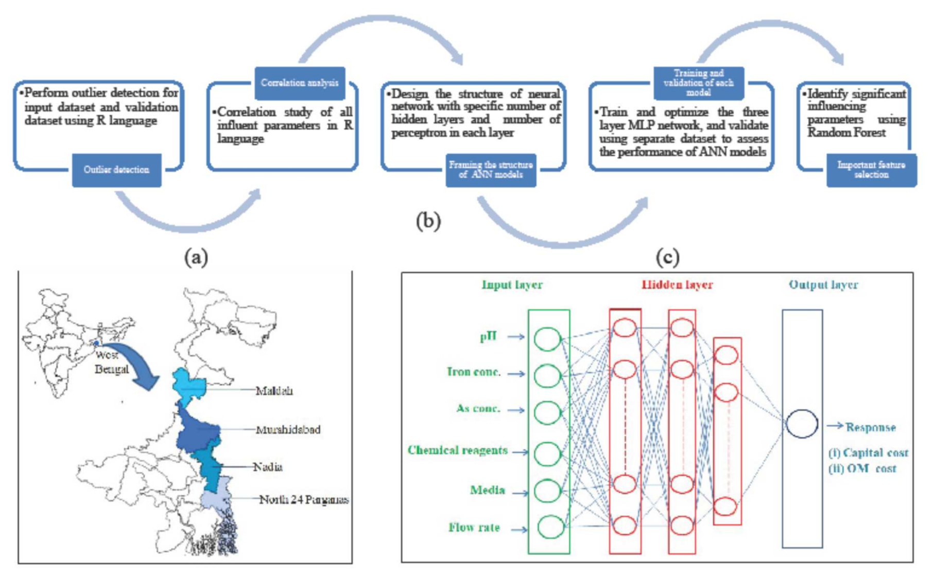
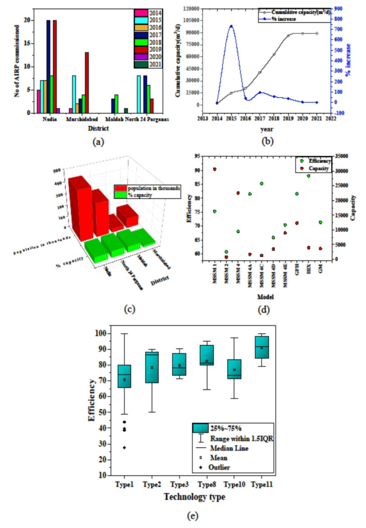
3.1. Overview of AIRP Schemes in the Study Area

West Bengal, one of the most affected states of India, has adopted significant measures for arsenic decontamination in drinking water. Some of the techniques adopted are activated laterite based arsenic filter [36], well-head arsenic removal units [37], Arsenic Removal Plants (ARPs) based on ZVI (from corrosion of iron nails) [38], and ArsenXnp, a hybrid anion exchanger in well-head arsenic removal systems [39].
The study area has been selected as 27 blocks of four districts (Nadia, Maldah, Murshidabad, and North 24 Parganas) in West Bengal (Figure 1a), where a pronounced arsenic prevalence is reported, and piped water supplies from groundwater sources are necessarily associated with arsenic iron removal plants (AIRPs) comprising various technologies. The data from existing and ongoing AIRPs, including plant location, population served, flow rate, plant running hours, technology, raw water parameters, effluent water quality, date of commissioning of each scheme, chemicals used, capital cost, and annual operation and maintenance costs (electricity, chemical, and other) in 136 plants installed and maintained by the Public Health Engineering Department, Govt. of West Bengal, India are represented in this study. Among the technologies implemented so far in the study area, adsorption combined with coagulation and filtration is widely adopted with different media and coagulant combinations. Raw water quality parameters depending on sources varied widely from scheme to scheme. The iron and arsenic content of inlet water changed from 0.1 mg/L to 9.7 mg/L and 1µg/L to 1550 µg/L, respectively. A wide range of variation for turbidity, total hardness (TH), and total dissolved solids (TDS) was observed, ranging from 0.1 to 98 NTU, 108 to 508 mg/L of CaCO3, 111 to 603 mg/L, respectively; pH maintained a range of 5.9 to 8.8 throughout the sampling period. AIRPs commissioned between 2014 and 2021 are considered in the data analysis.
An extensive statistical analysis and numerical modeling were carried out to study the efficiency of technologies as well as their capital cost (CC) and operation and maintenance (OM) cost. Non-linear regression was applied to the data for univariate data analysis, which comprised the following objectives:
  • Current economic indicators.
  • The year-on-year increase in cumulative capacities till the current year.
  • The cumulative capacities of arsenic-free water across the study area.
  • Primary oxidation and disinfection methods.
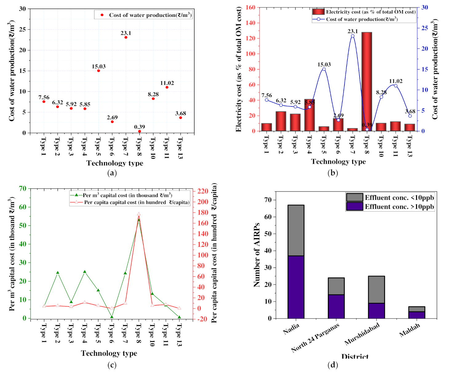
  • Cost of arsenic-free water production depending on technology and plant capacity.
Furthermore, the pair-wise correlation between the major influencing parameters (arsenic and iron concentration, turbidity, TDS, pH, TH of raw water) was estimated. Subsequently, a data analysis framework (Figure 1b) with deep neural and random forest-based multivariate prediction modeling was conducted to demonstrate the impact of various processes and water quality parameters on the technical and economic aspects of the AIRPs in the study area.

3.2. Multivariate Modeling of AIRP Performance and Cost

A large set of treatment plant data was used to prepare a multivariate model delineating the influence of impactful parameters as factors in the cost and technical aspects of AIRPs as a response. The proposed modeling approach consisted of framing a comprehensive dataset (a large dataset of the process, as well as the performance and environmental parameters in the study area), screening the data through identifying outliers (as mentioned below), and the effective utilization of screened data to prepare significant predictive models. The protocol of the modeling study of the present study lies in the following aspects in chronology as depicted in the flowchart (Figure 1b):
  • Organizing the collected database in terms of independent variables as significant technological and water quality parameters concerning the cost indicator and plant performance as responses.
  • Data screening by outlier detection using the R package (‘OutlierDetection’).
  • Correlation study for all the variables in the screened dataset using the R language.
  • Development of a robust prediction model from the screened dataset through ANN in a python environment. Here, the utilization of the dataset concerning the formation of a predictive model consisted of two perspectives. First, the model preparation and calibration (training, testing, and cross-validation) were conducted from 90% of the screened data. However, around 10% of the total screened data were kept separate as new data for validating the predictive model. This approach of validation ensures the applicability of the developed model in any field condition of different scenarios, which was established with a separate dataset, as mentioned above.
  • An RF-based classification algorithm was applied to the entire screened data in a python environment to identify the major influential parameters of the performance indicators.
Before the data is fed as input to the neural network, all inconsistent (repetitive data or data consisted of anomalies due to system error, such as measurement error, plant operational error etc.) and incomplete instances were removed manually (approximately 10% of the total observed data), and no duplicate records were found in the dataset. An outlier detection package in R, based on the dispersion method, was used to remove all the outliers to avoid bias and change in the fit of the curve. This method creates an actual dispersion matrix considering all the data, and a Leave-One-Out (LOO) dispersion matrix without considering the current data point chosen at random. Subsequently, the difference between the matrixes, known as the bootstrapped cut-off score; based on this score, a particular data point is labeled as an outlier [40]. The Pearson correlation method was conducted using R to determine the inter-relationships among the input variables.
To predict and model complex relationships among several factors and responses in a dataset, neural networks require training or calibration for learning from data instead of utilizing a mathematical relationship. A feed-forward multi-layer perceptron (MLP) network was employed for the multivariate nonlinear data analysis. In the present study, the input layer consisted of various independent parameters, such as pH, flow rate, chemical reagents, iron, and arsenic concentration, and the output layer consisted of efficiency and cost parameters to predict them as responses.
The ANN is a computing paradigm. It was first used in cognitive science and engineering. Neural networks introduced as efficient modeling and forecasting tools; are less sensitive to the error term assumptions and tolerant to noise and chaotic components [41]. This modeling technique makes it possible to accommodate additional constraints that may arise in the application, making it a highly flexible function that approximates data [12]. The data were divided into training and testing using “train-test-split” from the sklearn library as a Python package [42]. The neural network was trained with 75% of data (20% of training data for cross-validation), and 25% of the dataset is kept for testing. While framing the prediction model of economic parameters, the CC and OM cost data was modeled, instead of using any of the individual economic indicators mentioned in this study.
The deep neural model architecture is represented in Figure 1c, having three hidden layers and using Keras sequential class to build the models in a python environment. The argument required for compiling the Keras model is “adam”, with a learning rate of 0.001. A batch size of 24 and 200 epochs was considered for each model. The number of nodes in each layer changed from 20 to 100 at intervals of four. The number of layers and the nodes in each layer varied to obtain the maximum value of the coefficient of determination and the minimum value of the error function. Moreover, an analysis of variance (ANOVA) was also carried out to understand the coherence between the two groups (predicted and actual values), with a null hypothesis that their means are significantly different from each other.
The RF regression model initiates a random selection of variables with replacement, (bootstrapping), which decreases the correlation between individual trees, leading to diminished variance when the trees are aggregated [18]. Next, the max feature is selected, which is the number of various predictors to try at each node. The selection of smaller values of the max feature prevents the overfitting of the data. Subsequently, the total number of regression trees of the original dataset (ntree) is selected based on the bootstrapped sample. Afterward, the numbers of the decision trees are constructed using the recursive partitioning technique. The selection of max feature and ntree is performed using a greedy algorithm to optimize the cut-off value (split point) based on the squared error loss [17,18]. The feature importance is selected with a majority of the vote from each tree and aggregating the result of all the decision trees. The tuning parameters, max feature, ntree, and depth of the tree are optimized for the important feature selection of CC, OM cost, and removal efficiency models. All the RF computation is performed in python using the “RandomForestRegressor” package in the sklearn library.

4. Results and Discussion

4.1. AIRP Capacity by Region

The number of AIRPs commissioned from 2014 to 2021 in the study area is represented in Figure 2a. Out of 136 operational AIRPs in the study area, there are 72 numbers of AIRP alone in Nadia district, which accounts for 52% of the AIRP plants. AA with FeCl3 is the major technology used in 64 schemes out of 136, indicating that this technology is a preferred choice. This technology includes all the large operational plants having a capacity of more than 1250 m3/d across the regions, 37% of the total capacity. Overall, there is an increasing trend towards the cumulative capacity of operational AIRPs throughout the study area, from 1770 m3/d in 2014 to 89,034 m3/d in 2021, with an additional plant capacity of 464 m3/d in progress. The objective of providing arsenic-free water to the people through piped water supply schemes (WSS) eventually led to an increasing trend in AIRP capacity with an average escalation rate of 120% between 2014 and 2021. The year-on-year percentage increment in cumulative capacity peaked in 2015 (733%), indicating an increase of 12,978 m3/d from 1770 m3/d within a year. The rate of per year increase afterward showed a downward trend, with the lowest percentage of cumulative capacity increase in 2021 (0.07%) as shown in Figure 2b.
The total capacity of the AIRPs in the Nadia district is 47,809 m3/d, which accounts for 53% of the total installed capacity of AIRPs in the study area, serving 39% of the population. In the Maldah district, a population of 65,190 is served with a cumulative plant capacity of 2662 m3/d, which holds 3% of the total AIRP capacity. Figure 2c depicts the distribution of the population and the AIRP capacity in every district in the study area. The uneven distribution of AIRPs is associated with several surface water supply projects running in the study area without AIRPs, as the prevalence of arsenic in the surface water is negligible. Dharani WSS of North 24 Parganas district has a maximum AIRP capacity of 4900 m3/d. The minimum capacity recorded is 28 m3/d in Ramchandrapur WSS, in zone-1 of the Murshidabad district.

4.2. Implemented Models for AIRP Projects

Several AIRP models are adopted based on site suitability, raw water quality, reagent availability, ease of operation, and maintenance fulfilling local citizens’ requirements. These models are modified to improve their functionality and efficiency over time. The details of the process flow diagram, the reagents used, and the technology type against the specified models are listed scheme-wise in Table S1 of the Supplementary material. The average efficiency of the different models is represented in Figure 2d. The Modified Sujapur Sadipur Model (MSSM) is the most commonly adopted model, accounting for 78% of the total capacity (86 plants out of 136). The type I version of this model comprises an oxidation chamber, coagulation, and a flocculation unit attached to a plain sedimentation tank, which eventually passes the water to a rapid gravity filter (RGF) and a polishing unit (PU) before the water is stored in a clear-water reservoir (CWR). In its type II version, the flocculation and sedimentation unit is used together as a clariflocculator, with an efficiency of 60%, 15% less than type I, while the arrangements of other units remain the same. The most efficient model of this MSSM series, MSSM IVC, reports an efficiency of 85%, which modifies the arrangement slightly, replacing the RGF with a pressure filter and two numbers of contact clarifiers instead of one conventional clarifier. Among all the models installed, it was observed that the hybrid ion exchange (HIX) model exhibited the highest removal efficiency, of 88%. The next most efficient model was granular ferric hydroxide (GFH), with an efficiency of 81.6%.

4.3. Current Field Scale Arsenic Removal Technologies

The leading technologies employed in the plants are adsorption combined with coagulation, adsorption with gravity, or pressure filtration, wherein pretreatment with oxidation is associated with every case. The plants are mainly based on three types of adsorption media; AA, GFH, and HIX. Seven varieties of coagulating agent, viz. alum, alum with ferric chloride, alum with ferrous sulfate, ferric chloride, ferrous sulfate, sodium sulfide, and sodium aluminate are predominately used in combination with media. The classification of the different technologies is presented in Figure S1. The technical details of the AIRPs for each scheme are described in Table S1 of the Supplementary Materials.
AA with FeCl3 being the major technology combination serves 49% population with a cumulative plant capacity of 55,802 m3/d, as shown in Figure S2. The other widely used combination is AA (adsorbent) and alum combined with FeCl3 (coagulant), which is employed in a plant capacity of 5249 m3/d, with population coverage of 15% in the study area. AA and alum with FeSO4were observed to feature a capacity of 4546 m3/d, but serving half of the population, as does the combination of AA and alum with FeCl3. Other minor adsorbent coagulant combinations include AA with alum, AA with FeSO4, HIX with FeCl3, HIX with FeSO4, GFH with NaAlO2, and GFH with Na2S, contributing 26% of total capacity, which serves 29% of the total population considered (Figure S3).
The data shows 50 schemes with removal efficiency between 50% and 75%, with a cumulative capacity of 40%. Only five schemes report 100% arsenic removal, four of which are AA-based. GFH with Na2S exhibits the highest removal efficiency of 95% employed in only one scheme. AA with FeCl3 combination reports the least average efficiency, of 71%, and has a wide range, from 28% to 100%, as depicted in Figure 2e, although some data displaying lower efficiency (below 44%) ranges are considered outliers in the Box plot. The next most predominant technology, the combination of AA with alum and FeCl3 as a coagulant, offers an average removal efficiency of 79%. HIX with FeCl3 removes arsenic with 91% efficiency, with a combined capacity of 3864 m3/d.
AIRPs consistof a pre-treatment unit of oxidation to convert As(III) to As(IV) for the efficient removal of total arsenic. Chlorination, which also acts as a disinfectant, is used for oxidation purposes. Sodium hypochlorite is predominantly used as an oxidizing agent, pre-treating 62% of total AIRP capacity, succeeded by calcium hypochlorite, which contributes 30% of the total capacity. The other minor oxidant reported is Na2S, which is mostly used with GFH.
The raw water quality parameters have a significant impact on arsenic removal efficiency. However, plant performance is influenced by several operational parameters and desired effluent standards as well. In this context, the univariate analysis on several raw water quality parameters and efficiency of AIRPs could barely exhibit a definite relationship. Nevertheless, the raw water quality parameters also feature some interactive effort, which is further represented in the surface plot of the initial arsenic and iron concentrations, TH and TDS, concerning the arsenic removal efficiency. It was reflected that higher iron and arsenic concentrations promote higher removal efficiency (Figure 3a), whereas the initial arsenic concentration with TH and TDS could not infer any defined relationship with arsenic removal efficiency (Figure 3b,c).
The global scenario on field-scale arsenic removal technologies from different studies exhibited an efficiency of more than 80% of oxidation-based or coagulation-based systems, which is also reflected from the present study in various treatment plants. However, the adsorption-based system demonstrated a wide variation, depending on the adsorbent used. Furthermore, different plants in the present study performed at a wide range of efficiency levels, as several technical and environmental factors are also responsible for the performance of adsorbents. Moreover, a combination of technologies, such as oxidation/coagulation-precipitation followed by adsorption, may also determine the performance efficiency, depending on the extent of treatment employed for a particular technology.

4.4. Economic Indicators in Current AIRPs

Concerning the financial aspects of AIRPs, several economic indicators used in the present study are water production cost per m3, per capita capital cost, and per m3/d capital cost, which depends on the technology adopted, the capacity of the plant, and types of adsorbents used. The average cost of water production for plants with a capacity of more than 1250 m3/d is ₹2.74 per m3 ($1 US ≈ ₹70 IN). From 2014 until the time of writing, the lowest water prices are reported for schemes with GFH as media, where both iron and arsenic treatment units are based on adsorbent column, with a cumulative capacity of 6152 m3/d. The lowest price noted is ₹0.19 per m3 for Karimpur-Jalangi WSS, in the Nadia district. The highest water price is for Bajitpur WSS, in the North 24 Parganas district, which uses GFH with FeCl3 as the coagulant, at ₹23.17 per m3 with a capacity of 540 m3/d.
The highest and lowest average production costs of ₹0.39 per m3 and ₹23.1 per m3 were reported in 2019 and 2017, respectively, for GFH-based technologies (Figure 4a). The most widely deployed combination, AA with FeCl3, features an average water production cost of ₹7.56 per m3. Other coagulants, such as FeCl3 with alum and FeSO4 with alum and AA as media, reports average production costs of ₹6.32 per m3and ₹5.92 per m3, respectively. The production cost using alum-based coagulation techniques is ₹5.85 per m3, whereas alum together with FeCl3 or FeSO4 exhibits a further reduction in the average cost by 16.4% and 60.6%, respectively.
AA-based schemes report a wider range of price, from ₹60.71 per m3 to ₹1.57 per m3, as compared to HIX (₹3.68 per m3 to ₹11.02 per m3) and GFH (₹0.39 per m3 to ₹23.1per m3) as media. The production cost is inversely proportional to the capacity of the plant. The average cost of water varied from ₹26.98 per m3for plants with a capacity of less than 100 m3/d to a minimum of ₹1.78 per m3 for more than 1500 m3/d capacity. AIRP of Dhalani WSS (4900 m3/d) shows a water price of ₹1.57 per m3, while Ramchandrapur WSS (28 m3/d) requires a production cost of ₹30.69 per m3. A comparison between the electricity cost (as % of total OM cost) and the cost of unit water production is plotted in Figure 4b.
The capital costs feature a maximum value of 44.76 million Indian rupees for GFH-based plants and a minimum of ₹0.1 million for AA with FeCl3.The capital cost per m3/d (₹52.85 per m3/d) and the per capita capital cost (₹17.7 thousand per capita) are both highest for AIRPs where only GFH is used as a coagulant (Figure 4c). The capital cost per m3/d and the capital cost per capita is lowest for HIX- and NaAlO2-based schemes, priced at ₹0.48 per m3/d and ₹0.03 thousand per capita, respectively.

4.5. Safety and Testing Status of AIRPs

A total of 64 schemes deliver treated water with a median effluent arsenic concentration greater than the BIS standard of 10 µg/L during low-maintenance periods (Figure 4d). The highest concentration of arsenic in treated water is 67 µg/L, in Teinpur WSS (124 m3/d), in the Nadia district. A total of 37 schemes that supply water with arsenic concentrations higher than 10 µg/L in the Nadia district were investigated. However, on the safer side, only 2% of the population from the scheme coverage is supplied with treated water with an arsenic concentration of more than 50 µg/L. In all four districts, 53.38% of the total capacity is supplied with treated water with an arsenic concentration of more than 10 µg/L.
Every AIRP is tested periodically to assess the consistency of its treated water standards. The frequency of testing varies from once a month to once a year. Only 19 out of 130 plants test their effluent over a period less than or equal to 30 days, whereas 60% of plants perform the testing between the period of 30 to 60 days, as shown in Figure S4. A total of 11 AIRP test their effluent less than once a year.

4.6. Benchmarking Presents Arsenic Management with Global Scenario

An insight into the technical and financial aspects of field-scale arsenic removal plants around the globe exhibits the applicability of conventional oxidation, coagulation, precipitation, or adsorption-based systems. Although several review papers highlighted [1,28] the overall details of ARPs, systematic in-depth studies on their performance and costs, addressing their environmental and process parameters, have seldom been conducted. This study observed a similar trend concerning the implementation of technology and the corresponding process performance. However, the comparison of the financial aspect with the overall scenario may be undermined due to data insufficiency and different technical and socio-economic factors. Nevertheless, the cost of treatment in the study area is grossly comparable to other places across the globe.

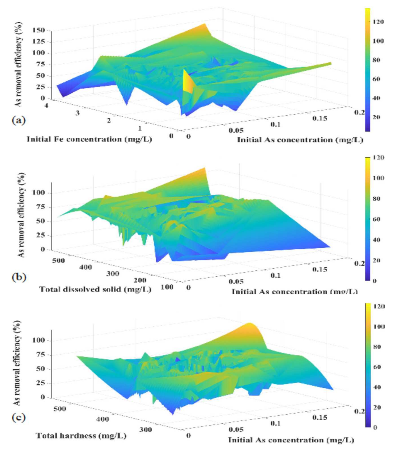
4.7. Prediction Models and their Applicability

4.7.1. ANN Study

The correlation matrix for various influent parameters, presented in Figure 5a, does not reflect a significant correlation among these parameters. Consequently, all the variables are considered to frame the prediction models of CC and OM costs using a neural network. While varying the activation function during the model formation, the hyperbolic tangent function exhibited better accuracy than the rectified linear unit (ReLU). The data screenings were conducted for separating the outliers before applying to the neural network model. However, the characteristic of the dataset is a major guiding factor for deciding the preferred loss function. Similarly, the loss functions were chosen as a mean absolute error (MAE) and mean square error (MSE), among which MAE exhibited better results for the optimization of the modeling parameters. The optimum ANN architecture for both the models was found to be a three-layered neural network with model structure 8-2X-X-0.5X-1 (eight input variables, 2X, X and 0.5X perceptrons in the first, second, and third hidden layer respectively, and one output layer;, X being the number of perceptrons).
The optimum network architecture is considered with 184–92–46 as the number of perceptrons for the first, second, and third hidden layers, respectively (Figure 5b). The R2 value and MAE concerning the optimized CC model are 0.72 and 4.41, respectively, for the overall dataset. Furthermore, the adequacy of the model was tested with the ANOVA for the predicted and actual values of the model. The ANOVA for the overall dataset of the optimized CC model displayed a high F value (5830.94) and low p-value (p < 0.001; corresponding to 99% confidence interval), as shown in Table 1. In total, 10% of screened data that were kept to validate separately for performance assessment (validation dataset) exhibited an R2of 0.67. Additionally, the ANOVA of the validation dataset for the CC model demonstrated an F value of 503.184, and the p-value was (p < 0.001), establishing its applicability.
The optimal number of perceptrons taken for the OM cost model is 128-64-32, which represents the number of perceptrons for the first, second, and third hidden layers, respectively (Figure 5c). The optimum R2 and MAE for the overall OM cost model were 0.98 and 0.26, respectively. The ANOVA for the overall dataset exhibited the highest F value, of 136,954, and a low p-value (p < 0.001), proving the models to be adequate. Further, the validation dataset exhibited a maximum R2 value of 0.98 and an MAE value of 0.26. The F statistic reported a value of 15,062.6, evaluating the statistical significance of the model.
The Pearson’s correlation coefficient of the optimized prediction model is depicted in Figure 5d–k for the training, testing, overall, and validation datasets. The R2 value found in every case was in good agreement with the adjusted R2 for all the models, implying an adequate amount of predictors used for modeling. Additionally, a set of error functions (sum of the square of the error (SSE), the sum of absolute error (SAE), MSE, MAE, the sum of absolute error (SAE), average relative error (ARE), hybrid fractional error function (HYBRID), and Marquardt’s percent standard deviation (MPSD)) were also evaluated for every model as performance indicators. The SSE, SAE, MSE, MAE, ARE, HYBRID, and MPSD obtained for the CC and OM cost model validation sets are presented in Table 2.
A prediction model for removal efficiency was also attempted, and poor values of performance indicators were obtained. The inadequacy of this model may be attributed to the fact that the variation of the treatment process parameters and the variation of the operation and maintenance parameters concerning the inlet water quality were rarely conducted. However, the adjustment of those process parameters was primarily targeted to achieve a treated water quality below the drinking water quality standard. Furthermore, the unavailability of some significant information, such as backwash frequency, the duration of backwashing, the interval between changes of media, and other such maintenance databases, may also undermine the accuracy of the removal efficiency-based prediction model.

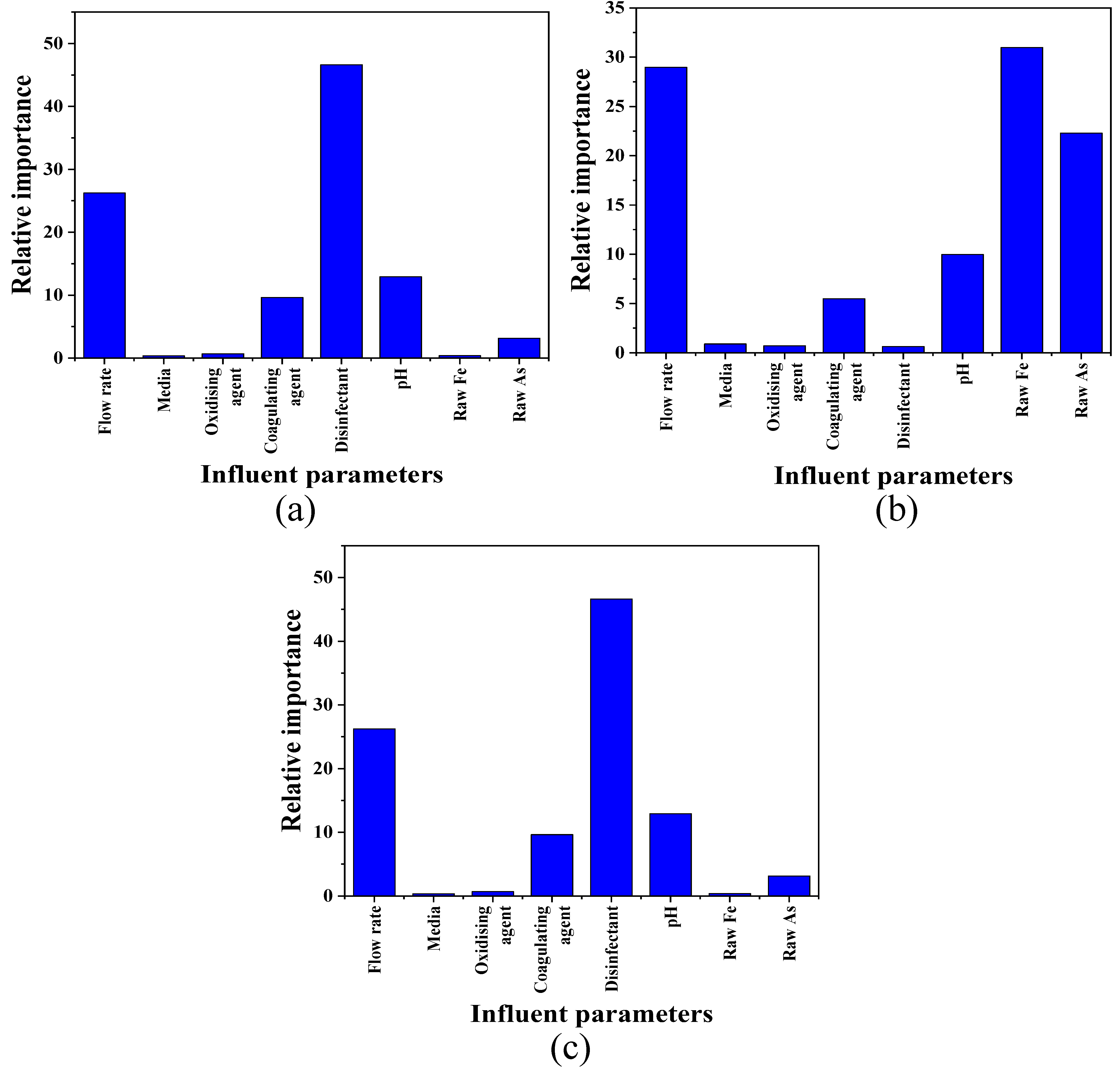
4.7.2. Important Feature Selection by RF

The maxfeature value was optimized as eight, which is the number of input variables. The optimum number of ntree was 300, above which there was no significant decrease in error value. The initial depth of the tree is considered as three, and an insignificant change in the importance of variables was observed on a further increase of the depth from four. The decision trees for CC, OM cost, and removal efficiency are shown in Figure S5 to visualize the regression models for the selection of important variables of these responses. Every node represents a specific condition based on the feature value, except for the leaf nodes, which represent the final value of the prediction. The MSE value decreases as we near the leaf nodes. ‘Samples’ indicates the number of observations in the node and the predicted value for each node is represented by ‘value’. Here, the prediction accuracy was selected from randomly shuffled variables, out of the superset, while keeping the rest others unaltered. In each case, the prediction accuracy of the shuffled data was measured and the mean decrease across all the trees is reported. The relative significance depends on their capacity to alter the accuracy of the prediction model. The lists of important variables for capital cost are disinfectant (39.67%), flow rate (33.79%), and oxidizing agent (21.87%). In contrast, the influencing variables for OM cost are disinfecting agent (46.63%), flow rate (26.23%), pH value (12.93%), and coagulant (9.64%). The trivial relative importance of media for OM cost may be attributed to the fact that the replacement of exhaust media or the replenishment of its capacity is devoid of adequate frequency. The analysis of the removal efficiency revealed flow rate, iron and arsenic content in influent water, pH value, and coagulating agent with % relative importance of 28.97%, 30.99%, 22.30%, 9.99%, and 5.49%, respectively, as principal parameters. The relative importance of the considered parameters for each model is shown in Figure 6.

4.7.3. Applicability of Machine Learning Based Framework

In this study, both univariate and multivariate data analyses were performed, considering the impact of the individual parameters and establishing relationships among several influencing parameters with the responses, to deliver financial guidelines for the capital and OM costs of proposed and existing projects. AIRP statistics and model prediction tools are important to understand the trend of key parameters, such as production capacity, technology, cost, and treatment efficiency. The prediction model arrived from the proposed framework along with the identification of important process parameters may prove a hand-on-tool for policymakers and potential investors to support the fair financial assessment of the gross capital budget for the implementation of AIRPs, concerning various environmental and process conditions. The understanding of this evaluation provides insights through which OM agencies can bridge the gap between plants’ OM costs and the predicted OM costs for current operational plants. Furthermore, the lower costs involved in operation and maintenance compared to the prescribed cost model may indicate inadequate chemical dosing and infrequent media replacement. Our study also advised how to set process parameters, adequate frequency of system modification in terms of media replacement, regeneration of media concerning the variation of water quality, flow, and other environmental factors. It manifests an opportunity for technology modification to have the utmost impact in the future. This study integrates technical and economic aspects to assist future planning and process improvement.

5. Conclusions

The extensive data survey carried out for 136 AIRPs from four districts in West Bengal is utilized effectively to prepare a comprehensive database to appraise the present status of arsenic remediation in significant arsenic-affected zones and the techno-commercial assessment of various technologies employed in AIRPs. The statistical assessment concludes that there was a steady rise of 120%, in the average cumulative capacity of AIRPs in the study area from 2014 to 2021. Among the implemented models, the MSSM series accounted for 78% of the total capacity. The maximum removal efficiency obtained was 100%, reported for AA-based technologies in four plants. In particular, AA with FeCl3 was found to be the most widely used technology, including all the large operational plants (capacity more than 1250 m3/d), across the studied region, with a cumulative capacity of 55,802 m3/d. The predominant pre-treatment method reported was oxidation with sodium hypochlorite, which also acts as a disinfectant. AA with FeCl3 demonstrated an average water price of ₹7.56/m3. The lowest average cost of water production was reported for GFH-based technology (₹0.39/m3), whereas both the capital cost indices exhibited the highest values for this technology: the capital cost per m3, which was ₹52.85 per m3, and the capital cost per capita, as ₹17.7 thousand/capita.
A systematic application of a machine learning-based novel framework along with the identification of outliers and the inter-relationships among the process parameters, was conducted on a large set of field data. The neural network was found to be an efficient tool to model both the cost indices with remarkably high R2 values; 0.7286 and 0.9844 for the CC and OM cost models, respectively. The high F values (5830.94 for the CC model and 136,954 for the OM model) obtained show the applicability of the models in practical scenarios. The results of the ANOVA and error functions exhibited the significance of the predicted model. In addition, a random forest regression model was optimized to select important process parameters affecting CC, OM cost, and removal efficiency. Disinfectant predominated as the most important parameter for both the cost models, with 39.67% and 46.63% relative importance for the CC and OM cost models, respectively. Iron content (30.99%) and flow rate (28.97%) were found to be of higher importance in the case of removal efficiency compared to other factors. The present study of univariate and multivariate analyses attempts to offer an organized approach to elucidate the relationships among independent variables. Furthermore, random forest models were framed to note the major influencing variables adding credibility to the work. Deep neural network-based multivariate models may prove to be an efficient tool for field engineers and policymakers to predict the cost indices in different field conditions integrating the techno-economic aspects of AIRPs.

Supplementary Materials

The following are available online at https://www.mdpi.com/article/10.3390/w13243507/s1. Table S1: Technical details of implemented schemes; Figure S1: Combination of technologies concerning media and chemicals; Figure S2: Contribution of major technologies to population and capacity (>90%); Figure S3: Contribution of minor technologies to population and capacity (<10%); Figure S4: Frequency of sampling of effluent water in AIRPs; Figure S5: Random forest model trees for (a) capital cost, (b) operation and maintenance cost, (c) removal efficiency

Author Contributions

A.B. has conducted field work and acquired the data. S.S. (Saswata Sahu) has reviewed the literatures. S.S. (Saswata Sahu) and V.T. have performed the coding and data analysis. A.B. and P.S.G. have helped in the conceptualization of the work. S.D. and S.S. (Soumyajit Sarkar) have done. S.S. (Saswata Sahu) and A.B. have written the manuscript with input from J.B. and others. A.M. has supervised the work. All the authors have discussed and finalized the manuscript. All authors have read and agreed to the published version of the manuscript.

Funding

This research was partly supported by data obtained from the Newton-Bhaba project FAR-GANGA [NERC (Govt. of UK) (NE/R003386/1) and DST (Govt. of India) (DST/TM/INDO-UK/2K17/55(C) & 55(G))] and DST WTI project TRIBUTE GANGA [DST/TMD-EWO/WTI/2K19/EWFH/2019/201 (G) & (C) Dated: 28.10.2020.

Institutional Review Board Statement

Not applicable.

Informed Consent Statement

Not applicable.

Data Availability Statement

Not applicable.

Acknowledgments

We would like to thank the Public Health Engineering Department, Government of West Bengal, for sharing information regarding the performance of Arsenic and Iron Removal Plants (AIRP) operating in the affected regions. We thank Biswajit Chakravorty, Himanshu Joshi, Debapriya Mondal, Ashok Ghosh, Nupur Bose, Chander Singh and Dipankar Saha for discussions. The opinions expressed in this paper however do not necessarily reflect those of any of the organizations or individuals whom we acknowledge here.

Conflicts of Interest

The authors declare no conflict of interest.

References

  1. Alka, S.; Shahir, S.; Ibrahim, N.; Ndejiko, M.J.; Vo, D.V.N.; Manan, F.A. Arsenic Removal Technologies and Future Trends: A Mini-Review. J. Clean. Prod. 2021, 278, 123805. [Google Scholar] [CrossRef]
  2. Garelick, H.; Jones, H.; Dybowska, A.; Valsami-jones, E. Introduction to Arsenic Contamination and Health Risk Assessment with Special Reference to Bangladesh. Rev. Environ. Contam. 2008, 197, 1–15. [Google Scholar] [CrossRef]
  3. Yadav, M.K.; Saidulu, D.; Gupta, A.K.; Ghosal, P.S.; Mukherjee, A. Status and Management of Arsenic Pollution in Groundwater: A Comprehensive Appraisal of Recent Global Scenario, Human Health Impacts, Sustainable Field-Scale Treatment Technologies. J. Environ. Chem. Eng. 2021, 9, 105203. [Google Scholar] [CrossRef]
  4. Kumar, A.; Roy, M.B.; Roy, P.K.; Wallace, J.M. Assessment of Arsenic Removal Units in Arsenic-Prone Rural Area in Uttar Pradesh, India. J. Inst. Eng. Ser. A 2019, 100, 253–259. [Google Scholar] [CrossRef]
  5. Mukherjee, A.; Fryar, A.E.; Scanlon, B.R.; Bhattacharya, P.; Bhattacharya, A. Elevated Arsenic in Deeper Groundwater of the Western Bengal Basin, India: Extent and Controls from Regional to Local Scale. Appl. Geochem. 2011, 26, 600–613. [Google Scholar] [CrossRef]
  6. Mukherjee, A.; Sarkar, S.; Chakraborty, M.; Duttagupta, S.; Bhattacharya, A.; Saha, D.; Bhattacharya, P.; Mitra, A.; Gupta, S. Occurrence, Predictors and Hazards of Elevated Groundwater Arsenic across India through Field Observations and Regional-Scale AI-Based Modeling. Sci. Total Environ. 2021, 759, 143511. [Google Scholar] [CrossRef] [PubMed]
  7. Chakraborty, M.; Sarkar, S.; Mukherjee, A.; Shamsudduha, M.; Ahmed, K.M.; Bhattacharya, A.; Mitra, A. Modeling Regional-Scale Groundwater Arsenic Hazard in the Transboundary Ganges River Delta, India and Bangladesh: Infusing Physically-Based Model with Machine Learning. Sci. Total Environ. 2020, 748, 141107. [Google Scholar] [CrossRef] [PubMed]
  8. Flora, S.J.S. Arsenic: Chemistry, Occurrence, and Exposure. In Handbook Arsenic Toxicology; Elsevier: Amsterdam, The Netherlands, 2015; pp. 1–49. ISBN 9780124199552. [Google Scholar]
  9. Bhakta, J.N.; Rana, S.; Jana, J.; Bag, S.K.; Lahiri, S.; Jana, B.B.; Panning, F.; Fechter, L. Current Status of Arsenic Contamination in Drinking Water and Treatment Practice in Some Rural Areas of West Bengal, India. J. Water Chem. Technol. 2016, 38, 366–373. [Google Scholar] [CrossRef] [Green Version]
  10. World Health Organization. Guidelines for Drinking-Water Quality: Incorporating the First Addendum; World Health Organization: Geneva, Switzerland, 2017; ISBN 9789241549950. [Google Scholar]
  11. Luong, V.T.; CañasKurz, E.E.; Hellriegel, U.; Luu, T.L.; Hoinkis, J.; Bundschuh, J. Iron-Based Subsurface Arsenic Removal Technologies by Aeration: A Review of the Current State and Future Prospects. Water Res. 2018, 133, 110–122. [Google Scholar] [CrossRef] [PubMed]
  12. Palani, S.; Liong, S.Y.; Tkalich, P. An ANN Application for Water Quality Forecasting. Mar. Pollut. Bull. 2008, 56, 1586–1597. [Google Scholar] [CrossRef] [PubMed]
  13. Antar, M.A.; Elassiouti, I.; Allam, M.N. Rainfall-Runoff Modelling Using Artificial Neural Networks Technique: A Blue Nile Catchment Case Study. Hydrol. Process. 2006, 20, 1201–1216. [Google Scholar] [CrossRef]
  14. Ozel, H.U.; Gemici, B.T.; Gemici, E.; Ozel, H.B.; Cetin, M.; Sevik, H. Application of Artificial Neural Networks to Predict the Heavy Metal Contamination in the Bartin River. Environ. Sci. Pollut. Res. 2020, 27, 42495–42512. [Google Scholar] [CrossRef] [PubMed]
  15. Ghosal, P.S.; Kattil, K.V.; Yadav, M.K.; Gupta, A.K. Adsorptive Removal of Arsenic by Novel Iron/Olivine Composite: Insights into Preparation and Adsorption Process by Response Surface Methodology and Artificial Neural Network. J. Environ. Manag. 2018, 209, 176–187. [Google Scholar] [CrossRef] [PubMed]
  16. Azqhandi, M.H.A.; Ghaedi, M.; Yousefi, F.; Jamshidi, M. Application of Random Forest, Radial Basis Function Neural Networks and Central Composite Design for Modeling and/or Optimization of the Ultrasonic Assisted Adsorption of Brilliant Green on ZnS-NP-AC. J. Colloid Interface Sci. 2017, 505, 278–292. [Google Scholar] [CrossRef] [PubMed]
  17. Lovatti, B.P.O.; Nascimento, M.H.C.; Neto, Á.C.; Castro, E.V.R.; Filgueiras, P.R. Use of Random Forest in the Identification of Important Variables. MicroChem. J. 2019, 145, 1129–1134. [Google Scholar] [CrossRef]
  18. Ghaedi, M.; Ghaedi, A.M.; Negintaji, E.; Ansari, A.; Vafaei, A.; Rajabi, M. Journal of Industrial and Engineering Chemistry Random Forest Model for Removal of Bromophenol Blue Using Activated Carbon Obtained from AstragalusBisulcatus Tree. J. Ind. Eng. Chem. 2014, 20, 1793–1803. [Google Scholar] [CrossRef]
  19. Uddameri, V.; Silva, A.L.B.; Singaraju, S.; Mohammadi, G.; Hernandez, E.A. Tree-Based Modeling Methods to Predict Nitrate Exceedances in the Ogallala Aquifer in Texas. Water 2020, 12, 1023. [Google Scholar] [CrossRef] [Green Version]
  20. Piroonratana, T.; Wongseree, W.; Assawamakin, A.; Paulkhaolarn, N. Chemometrics and Intelligent Laboratory Systems Classi Fi Cation of Haemoglobin Typing Chromatograms by Neural Networks and Decision Trees for Thalassaemia Screening. Chemom. Intell. Lab. Syst. 2009, 99, 101–110. [Google Scholar] [CrossRef]
  21. Hapfelmeier, A.; Ulm, K. A New Variable Selection Approach Using Random Forests. Comput. Stat. Data Anal. 2013, 60, 50–69. [Google Scholar] [CrossRef]
  22. Berg, M.; Luzi, S.; Giger, W.; Trang, P.T.K.; Viet, P.H.; Stüben, D. Arsenic Removal from Groundwater by Household Sand Filters: Comparative Field Study, Model Calculations, and Health Benefits. Environ. Sci. Technol. 2006, 40, 5567–5573. [Google Scholar] [CrossRef] [PubMed]
  23. Smith, K.; Li, Z.; Chen, B.; Liang, H.; Zhang, X.; Xu, R.; Li, Z.; Dai, H.; Wei, C.; Liu, S. Chemosphere Comparison of Sand-Based Water Fi Lters for Point-of-Use Arsenic Removal in China. Chemosphere 2017, 168, 155–162. [Google Scholar] [CrossRef]
  24. Katsoyiannis, I.A.; Mitrakas, M.; Zouboulis, A.I. Arsenic Occurrence in Europe: Emphasis in Greece and Description of the Applied Full-Scale Treatment Plants. Desalin. Water Treat. 2015, 54, 2100–2107. [Google Scholar] [CrossRef]
  25. Litter, M.I.; Alarcón-Herrera, M.T.; Arenas, M.J.; Armienta, M.A.; Avilés, M.; Cáceres, R.E.; Cipriani, H.N.; Cornejo, L.; Dias, L.E.; Cirelli, A.F.; et al. Small-Scale and Household Methods to Remove Arsenic from Water for Drinking Purposes in Latin America. Sci. Total Environ. 2012, 429, 107–122. [Google Scholar] [CrossRef] [PubMed]
  26. Jain, C.K.; Singh, R.D. Technological Options for the Removal of Arsenic with Special Reference to South. J. Environ. Manag. 2012, 107, 1–18. [Google Scholar] [CrossRef] [PubMed] [Green Version]
  27. Khalid, F. An Overview of Arsenic Removal Technologies in India. Invert. J. Renew. Energy 2017, 7, 5–16. [Google Scholar] [CrossRef]
  28. Kurz, E.E.C.; Luong, V.T.; Hellriegel, U.; Leidinger, F.; Luu, T.L.; Bundschuh, J.; Hoinkis, J. Iron-Based Subsurface Arsenic Removal (SAR): Results of a Long-Term Pilot-Scale Test in Vietnam. Water Res. 2020, 181, 115929. [Google Scholar] [CrossRef] [PubMed]
  29. Chen, J.; Wang, S.; Zhang, S.; Yang, X.; Huang, Z.; Wang, C.; Wei, Q.; Zhang, G.; Xiao, J.; Jiang, F.; et al. Arsenic Pollution and Its Treatment in Yangzonghai Lake in China: In Situ Remediation. Ecotoxicol. Environ. Saf. J. 2015, 122, 178–185. [Google Scholar] [CrossRef] [PubMed]
  30. Katsoyiannis, I.A.; Zikoudi, A.; Hug, S.J. Arsenic Removal from Groundwaters Containing Iron, Ammonium, Manganese and Phosphate: A Case Study from a Treatment Unit in Northern Greece. Desalination 2008, 224, 330–339. [Google Scholar] [CrossRef]
  31. Yaqub, M.; Lee, S.H.; Lee, W. Investigating Micellar-Enhanced Ultrafiltration (MEUF) of Mercury and Arsenic from Aqueous Solution Using Response Surface Methodology and Gene Expression Programming. Sep. Purif. Technol. 2021, 281, 119880. [Google Scholar] [CrossRef]
  32. Figoli, A.; Fuoco, I.; Apollaro, C.; Chabane, M.; Mancuso, R.; Gabriele, B.; De Rosa, R.; Vespasiano, G.; Barca, D.; Criscuoli, A. Arsenic-Contaminated Groundwaters Remediation by Nanofiltration. Sep. Purif. Technol. 2020, 238, 116461. [Google Scholar] [CrossRef]
  33. Chen, A.S.C.; Wang, L.; Sorg, T.J.; Lytle, D.A. Removing Arsenic and Co-Occurring Contaminants from Drinking Water by Full-Scale Ion Exchange and Point-of-Use/Point-of-Entry Reverse Osmosis Systems. Water Res. 2020, 172, 115455. [Google Scholar] [CrossRef] [PubMed]
  34. Cañas Kurz, E.E.; Hellriegel, U.; Figoli, A.; Gabriele, B.; Bundschuh, J.; Hoinkis, J. Small-Scale Membrane-Based Arsenic Removal for Decentralized Applications–Developing a Conceptual Approach for Future Utilization. Water Res. 2021, 196, 116978. [Google Scholar] [CrossRef]
  35. Parga, J.R.; Cocke, D.L.; Valenzuela, J.L.; Gomes, J.A.; Kesmez, M.; Irwin, G.; Moreno, H.; Weir, M. Arsenic Removal via Electrocoagulation from Heavy Metal Contaminated Groundwater in La Comarca Lagunera México. J. Hazard. Mater. 2005, 124, 247–254. [Google Scholar] [CrossRef] [PubMed]
  36. Mondal, S.; Roy, A.; Mukherjee, R.; Mondal, M.; Karmakar, S.; Chatterjee, S.; Mukherjee, M.; Bhattacharjee, S.; De, S. A Socio-Economic Study along with Impact Assessment for Laterite Based Technology Demonstration for Arsenic Mitigation. Sci. Total Environ. 2017, 583, 142–152. [Google Scholar] [CrossRef] [PubMed]
  37. Sarkar, S.; Gupta, A.; Biswas, R.K.; Deb, A.K.; Greenleaf, J.E.; Sengupta, A.K. Well-Head Arsenic Removal Units in Remote Villages of Indian Subcontinent: Field Results and Performance Evaluation. Water Res. 2005, 39, 2196–2206. [Google Scholar] [CrossRef]
  38. Nath, K.J.; Sharma, V.P. Water and Sanitation in the New Millennium; Springer: New Delhi, India, 2017; pp. 1–254. [Google Scholar] [CrossRef]
  39. Sarkar, S.; Blaney, L.M.; Gupta, A.; Ghosh, D. Use of ArsenXNp, a Hybrid Anion Exchanger, for Arsenic Removal in Remote Villages in the Indian Subcontinent. React. Funct. Polym. 2007, 67, 1599–1611. [Google Scholar] [CrossRef]
  40. R Core Team. A Language and Environment for Statistical Computing: R Foundation for Statistical Computing; R Core Team: Vienna, Austria, 2020; Available online: https://www.R-project.org/ (accessed on 25 August 2021).
  41. Othman, F. Reservoir Inflow Forecasting Using Artificial Neural Network. Int. J. Phys. Sci. 2011, 6, 434–440. [Google Scholar] [CrossRef]
  42. Python Software Foundation. 2020. Available online: https://www.python.org/psf/ (accessed on 20 August 2021).
Figure 1. (a) Study area, (b) flowchart of proposed framework, (c) ANN architecture with variable number of perceptron in three hidden layers.
Water 13 03507 g001
Figure 2. (a) District-wise number of AIRP commissioned each year, (b) AIRP capacities in terms of cumulative installed capacity and year-wise % increase, (c) covered population (in thousands) and % capacity contribution in the study area, (d) capacity and efficiency of implemented models, and (e) box plot for efficiencies of major technologies (data source: Table S3 in Supplementary Materials).
Water 13 03507 g002
Figure 3. Interactive effect of (a) initial arsenic and iron concentration, (b) initial arsenic concentration and total dissolved solids, and (c) initial arsenic concentration and total hardness on arsenic removal efficiency (plotted from the influent and effluent data of AIRPs).
Water 13 03507 g003
Figure 4. (a) Unit price for production of arsenic free water, based on technology, (b) a comparison between energy cost (as % of total OM cost) and cost of unit water production, (c) per-m3 capital cost and per capita capital cost of technologies implemented, (d) number of AIRPs meeting effluent standard.
Water 13 03507 g004
Figure 5. (a) Correlation matrix for raw water parameters (circle size indicates the quantum of correlation). Variation of MAE and R2 with number of perceptron for (b) CC model, (c) OM model on validation dataset. Scattered plot for target and output for CC model on: (d) training dataset, (e) testing dataset, (f) overall model; and OM model on: (g) training dataset, (h) testing dataset, (i) overall model, and scattered plot for validation dataset of (j) CC model, (k) OM model.
Water 13 03507 g005
Figure 6. Relative feature importance of influent parameters for (a) capital cost, (b) operation and maintenance costs, (c) removal efficiency.
Water 13 03507 g006
Table 1. ANOVA of training and validation dataset of neural network model.
ModelSum of
Squares
DOFMean
Square
F Valuep ValueR2Adj R2
Model for CC
Model
Regression2,320,470.0412,320,470.045830.94<0.0010.730.73
Residual864,364.472172397.96
Total3,184,834.522173
Validation
Regression231,362.21231,362.2503.18<0.0010.680.67
Residual110,810.8241459.96
Total342,173242
Model for O & M
Model
Regression62,809.09162,809.09136,954<0.0010.980.98
Residual996.1121720.46
Total63,805.202173
Validation
Regression6568.2016568.2015,062.6<0.0010.980.98
Residual105.092410.44
Total6673.29242
Table 2. Error functions of each model.
Model 1 (CC Cost)Model 2 (OM Cost)
Error FunctionsModelValidationModelValidation
Sum of the square of the error1,177,617.43159,938.061155.35122.50
Sum of absolute error9598.531257.79565.8362.97
Mean square error541.43658.180.530.50
Mean absolute error4.415.180.260.26
Average relative error110.38130.062.492.48
Hybrid fractional error function15,844.9918,761.632.662.47
Marquardt’s percent standard19.9721.775.635.58
Publisher’s Note: MDPI stays neutral with regard to jurisdictional claims in published maps and institutional affiliations.

