
Analysis of Long-Term Shoreline Observations in the Vicinity of Coastal Structures: A Case Study of South Bali Beaches


1
Graduate School of Water Resources, Sungkyunkwan University, Suwon-si 16319, Korea
2
Directorate General of Water Resources, Ministry of Public Works and Housing, Jakarta 12110, Indonesia
*
Author to whom correspondence should be addressed.
Water 2021, 13(24), 3527; https://doi.org/10.3390/w13243527
Submission received: 28 October 2021
/
Revised: 6 December 2021
/
Accepted: 7 December 2021
/
Published: 9 December 2021
(This article belongs to the Section Oceans and Coastal Zones)
Abstract
:Recently, many rigid structures have been installed to cope with and efficiently manage coastal erosion. However, the changes in the coastline or isocenter and the movements of coastal sediment are poorly understood. This study examined the equilibrium shoreline and isocenter lines by applying a Model of Estimating Equilibrium Parabolic-type Shoreline (MeEPASoL) as an equilibrium shoreline prediction model. In addition, the inverse method was used to estimate littoral drift sediment transport from long-term beach profile observations. The movement of coastal sediments was analyzed using long-term beach profile observation data for three Indonesian beaches, namely, Kuta Beach for 13 years, Karang Beach in Sanur for 15 years, and Samuh Beach in Nusa Dua for 18 years. The littoral drift at every site was dynamically controlled by seasonal changes in the monsoon, the erosion and deposition patterns coupled with the presence of coastal structures, and limited sediment movement. Shoreline deformation in Kuta is generally backward deformed, with a littoral drift from south to north. In Sanur, the littoral drift vector carries sediment from the right and left sides and forms a salient behind the offshore breakwater. The littoral drift at Nusa Dua is dominantly from south to north, but the force of sediment transport decreases near the breakwater towards the north. Furthermore, the methods applied herein could aid the development of strategic coastal management plans to control erosion in subcells of coastal areas.
1. Introduction
1.1. Background
In coastal areas, project planning and design require quantitative knowledge of shoreline position changes. Using these data, analyses can be conducted to evaluate sediment budget, engineering modifications on the coast, variations in geomorphology, and future shoreline changes. Several methods can be used to obtain shoreline data, such as terrestrial measurements with beach profiles, aerial mapping, and light detection and ranging (LIDAR) [1,2,3] to obtain both short-term and long-term data. However, long-term shoreline data is more suitable for facilitating coastal management. Erosion rates represent long-term data, enabling future forecasts with estimated uncertainties [4].
Shoreline deformation in many areas has been formally evaluated without sufficient data from periodic coastal observations during project implementation, which has led to the serious deformation of the shoreline, threatening coastal structures and nearby coastal systems [5]. Coastal erosion is a global problem facing a number of nations worldwide [6,7,8,9,10]. In Southeast Asia, for instance, over the last 15 years (2000–2015), the coastline has experienced 5% deposition and 6% retreat, based on remote sensing data extraction [7]. In South Korea, coastal erosion has occurred since at least the 1990s as a result of the infrastructure influence, amount of river sediment flow, and other factors [11,12,13].
The high demand for residency in coastal areas has also led to the widespread coastal construction [13], such as the Pengambengan fishing port in the western part of Bali. These coastal harbors hinder longshore transport from the Indian Ocean, causing erosion in the downcoast area, as indicated by the collapsed seawall and scarp erosion [14]. Kuta Beach has experienced 100 m of erosion since the1960s, owing to littoral drift from the construction of Ngurah Rai Airport [15]. The natural process of sediment transport can also disturb coastal stabilization, such as the erosion at Nusa Dua.
Coastal and harbor structures, such as groins, detached breakwaters, and revetments, are often used for coastal protection to mitigate erosion originating from longshore sediment transport [16,17,18]. Longshore transport is often disturbed by the presence of these structures, such that sediment buildup occurs along the side of the updrift structure along with erosion in the downdrift direction. Material or sediment carried in the longshore direction causes sand movement from one cell to another, i.e., littoral drift. A coastal structure or harbor also changes the sediment loss rate and beach width [12]. In addition, an expansive beach absorbs wave energy and acts as a buffer to reduce damage from high waves [5]. It is thus vital to maintain the beach width to mitigate the risk of beach erosion.
In Bali, beaches have a fundamental societal role not only as tourist destinations [19] but as a place of religious events. However, they have suffered from erosion since the 1970s because of coral and sand mining, large-scale construction such as airport runways, hotels, restaurants, and other factors. Onaka et al. [15] surveyed Bali after the construction of artificial coastal structures by the Indonesian government and the Japan International Cooperation Agency (JICA) and found that the sand volumes at Sanur and Nusa Dua beaches were maintained. There was, however, a recession in the shorelines bordering rigid structures. Such structures, including groins, detached breakwaters, and artificial coral reefs, have been constructed in Bali, at Kuta Beach [20] and Nusa Dua Beach, for example [21], making it all the more critical to carry out regular and accurate measurements of sediment budgets along the coast and the prediction of shoreline changes due to previously built structure [22]. Long-term observations of waves, shoreline changes, beach profile deformation, and seabed quality are essential to mitigate beach erosion. Regrettably, the countermeasures to effectively cope with erosion pressure are currently limited [5].
The primary purpose of this study was to analyze shoreline deformation in response to littoral drift patterns on Kuta, Sanur, and Nusa Dua beaches in Bali. The effect of coastal structures and littoral drift on shoreline equilibrium was analyzed using the MeEPASoL program. The method used in this study took the inverse matrix concept developed by Lee et al. [5] to estimate the movement of sediment and the coastal seafloor due to shoreline changes, using long-term observation data. The shoreline was defined from the beach profile data based on the high-water level (HWL) position at Benoa Port. Littoral drift analysis was carried out based on long-term beach profile monitoring data for 13 years at Kuta Beach, 15 years at Sanur, and 18 years at Nusa Dua Beach. Long-term monitoring data were also used to assess the effects of seasonal changes in a littoral drift on long-term coastal stability. The method used in this study has previously been validated for the analysis of the movement pattern of the coastal seafloor at Kailua Beach, Hawaii, and the Gangneung area in South Korea using short-term observation data [5]. With long-term observation data, the methods used herein could offer a solution for developing strategic coastal management plans to control erosion in the causal areas subcell.
This paper consists of a brief introduction to shoreline changes due to coastal structures in Section 1. The characteristics of the study area, including existing structures, are provided in Section 2. The materials and methods, including the study site conditions, are in Section 3. Section 4 offers the results of the methods applied at each beach in accordance with the long-term observation data. A brief discussion explaining the results based on the theory and the new approach comprises Section 5 and is followed by the concluding remarks on this research project.
1.2. Shoreline Changes Due to Coastal Structures
Longshore sediment analysis can be integrated with the analysis of present structures in order to study shoreline changes [11]. The coastal sediment loss rate due to the construction also changes the width of the beach after the shoreline reaches equilibrium [12]. Static equilibrium conditions can be achieved if the volume of incoming sediment is the same as that of the outflowing sediment, but if these rates are unequal, erosion or accretion occurs [23].
To achieve an ideal or shoreline equilibrium, erosion prevention efforts are usually carried out in coastal areas by building coastal or harbor structures. However, the construction of these structures causes erosion from longshore sediment transport, disruption of longshore drift, downcoast erosion, and the trapping of sand on the updrift side of the structure [14,17]. The longshore transport that drives the littoral cell is correlated with the predominant waves [21], and the littoral morphology forms based on the sediment inflow and outflow.
Coastal protection structures can be perpendicular to the shoreline (groins) or parallel to the shoreline (detached breakwaters) [17]. Each type of structure has different effectiveness at handling erosion, as shown in Figure 1. For example, the effectiveness of groins depends on the length and spacing of groins relative to the width of the coast in the littoral zone (Figure 1b). Thus, a small space in areas with substantial variations in the direction of waves inhibits the movement of the littoral cell. However, if the length of the groins is increased, more sediment becomes trapped in the updrift region of the groins, leading to rapid erosion downcoast [17]. If the oblique angle of waves towards the coastline is more than 45°, it will cause an unstable shoreline to form a sand spit [14].
Shoreline perpendicular coastal protection structures are found on the Java coast, Indonesia, Wonpyeong and Wolcheon beach, Korea, and Cahaya beach, Malaysia [11,24,25]. At Wonpyeong beach, South Korea, the presence of Gungchon’s Port has impacted the coastal erosion, changing the wavefield in the study area and forming a new shoreline [11]. Meanwhile, in Nusa Dua, Bali, the existence of groin structures has caused beach erosion, although, in some sublittoral cells, the deposition occurs more rapidly than erosion [21]. Vaidya et al. [17] noted that groin length could be optimized based on the width of the surf zone since a long groin will increase erosion in the downdrift area. The width of this surf zone can act as a buffer by dampening wave energy, thereby reducing erosion damage [5].
Detached breakwaters have been proven to be able to form new salient (Figure 1a) in the sheltered zone of the structure and to reduce erosion in the downcoast area compared to groins, but they have other problems, such as increased water circulation in the sheltered basin, and rip currents between detached breakwaters installed in the same place [26]. In Kuala Terengganu coastline, Malaysia, the placement of breakwaters protects the shore from erosion but blocks longshore sediment transport such that it disrupts hydrodynamic processes in this area [25]. In Yeongrang Beach, South Korea, the presence of double headland on both sides of the coast encourages significant erosion in the center area [11]. However, the detached breakwater can reduce erosion in the downdrift, so it is usually combined with beach nourishment to prevent erosion, as was the case in Bali during the Beach Conservation Project in 2000 [15,17].
Several programs have been developed to identify the shoreline changes and the stability of headland-bay beaches (HBB). Among them, GENESIS (GENEralized model for SImulating Shoreline change) is widely applied to study shoreline rate changes based on the concept of a one-line model with the assumption that the beach profile is unchanged [27]. In 2018, Emily et al. [28] introduced a Digital Shoreline Analysis System (DSAS) to calculate shoreline rate changes and forecast shoreline changes over the next 10 or 20 years. More recently, DSAS has been applied to account for shoreline rate changes [29,30,31]. Terrestrial measurements for shoreline demarcation due to tidal action, coastal structures, and littoral drift movements are recommended to achieve the most accurate results [29].
To analyze the equilibrium position due to the influence of shoreline structures, the parabolic bay shape Equation (PBSE) concept developed by Hsu and Evans (1989) is widely used [11]. Based on the PBSE concept, many models have been developed to identify the stability of HBB, such as the model for equilibrium planform of bay beaches or MEPBAY [32] and the Model of Estimating Equilibrium Parabolic-Type Shoreline, MeEPASoL [21]. MEPBAY has been recognized widely in assessing beach stability [33,34,35,36,37,38]. However, in its application, there are some limitations of MEPBAY, such as; the subjectivity of determining downdrift control point [36] and multiple diffraction points in large structures or various headlands [35]. In MeEPASoL, the most probable offshore direction is determined by the wave phase potential in polar coordinates [21]. Thus, the downdrift tangent and control point obtained and applied in the PBSE is more accurate.
2. Characteristics of Study Areas
2.1. Study Areas
Bali is an island between Java and Sumbawa Island, Indonesia, and is famous for its beach tourism [39], especially for beaches located in the south, facing the Indian Ocean, as shown in Figure 2. These include Sanur, Kuta, Nusa Dua, and Tanah Lot beaches [21].
Despite their favorable economic aspects, beaches in Bali are currently experiencing erosion. Makfiya et al. [40] used a one-line model and found that the shoreline at Kuta Beach experienced erosion and accretion (with an erosion rate of 1–2 m/year for 25 years). Tsuchiya reported similar findings [41], showing that 100 m of Kuta Beach had eroded since the 1960s. Several solutions have been proposed to solve this problem.
The present study focused on Kuta beach, near Ngurah Rai Airport, located at 8°44′7.49″ S 115°9′45.48″ E and stretching for 676 m. Kuta Beach (Figure 2b) is more than 10 km from Legian, Seminyak, and up to the northern part of Kuta, which is located in Badung Regency, Bali. The D50 or grain size of sediments on Kuta Beach, based on an analysis conducted in 2008, is 0.20 mm. The grain size further north is finer [20]. The significant wave height in this area is approximately 1–3 m with a significant wave period of approximately 4–8 s [40]. The dominant wave direction is from the west-southwest in the wet season. Kuta experiences high refracted waves from the southwest [42].
Sanur Beach (Figure 2c) is located in Denpasar City and is 6 km long [43]. Waves at Sanur Beach are influenced by monsoon conditions, and the dominant wave direction is from the south-southeast. This beach has an average D50 of 0.61 mm, based on an analysis conducted in 2004 during the first sand nourishment [42]. The significant wave height in this area is 1.7–5.5 m, with a significant wave height of 16 s. The presence of coral off the coast of Sanur causes the coefficient of refraction on the coast of Sanur to be greater than that of Kuta on the southwest coast of Bali. In the present study, we analyzed the conditions of Karang Beach, Sanur, located between groins GN4 and G16, at 8°41′32.76″ S 115°16′1.03″ E, 250 m in length.
The wave conditions on Sanur and Nusa Dua beaches were not significantly different because both were located on the east coast of southern Bali; additionally, the same wave data source was used. The D50 at Nusa Dua Beach is 0.61 mm, based on data collected during the sand nourishment in 2003. For Nusa Dua Beach (Figure 2d), the study area was constrained to Samuh Beach (8°47′6.69″ S 115°13′36.89″ E), between groins GN1 and G9 with a length of 210 m. A summary of the characteristics of the study areas is presented in Table 1.
2.2. Existing Structures and Projects
To recover previously naturally sandy beaches, the Bali Beach Conservation Project Phase 1 was undertaken by the Indonesian government, financed by Japan. At Sanur, Kuta, and Nusa Dua, beach nourishment was carried out along with the construction of artificial coastal structures to minimize sand discharge by waves.
At Kuta Beach, to overcome erosion caused by the interruption of the longshore sediment transport process, owing to the construction of the Ngurah Rai Airport runaway, the Indonesian Ministry of Public Works and Housing constructed three units of breakwater buildings, as well as beach fillings. The study area selected was thus between two detached breakwaters, BWN1 and BWN2. In addition, there are two flat reef restorations in front of the beach at a distance of approximately 165 m that are parallel to the shoreline, as shown in the satellite image (Figure 3a).
Similar to Kuta Beach, there are coastal protection buildings in Sanur in the form of groins (Figure 3b) and offshore breakwaters [43]. The coastal structures include a T-shaped groin (GN4), an L-shaped groin (G16), and the offshore breakwater BWN1. The estimated dimensions of each structure are presented in Table 2.
In Nusa Dua Beach, the Indonesian government collaborated with JICA in 2001–2003 to carry out a beach nourishment project, along with the construction of several groins along the Nusa Dua coast, to prevent coastal erosion due to longshore drift [42]. There are a total of 17 sublittoral cells; however, only the area between groins GN1 and G9 was selected in this study to analyze the relationship between structures, littoral cell pattern, and shoreline deformation. GN1 and G9 are L-shaped groins.
3. Materials and Methods
3.1. Data Collection
Beach profile observation data were obtained from the Ministry of Public Works and Housing, Directorate of Water Resources, Indonesia. A summary of the data used in this study is given in Table 3. At Kuta Beach, the data used were collected during 2008–2021, only in the area with a beach length of 676 m from Bali Hai Hotel Kuta to Santika Hotel, Kuta, between BWN1 and BWN2. For Sanur beach, specifically Karang beach, the data were collected during 2004–2019; and for the Nusa Dua area, specifically Samuh beach, data were collected during 2003–2021. Cross-shore profile (Figure 4) data were X, Y, and Z position data from terrestrial measurements using the electronic total station. Position refers to the UTM 50S projection and WGS84 geodetic data. In addition, to define the shoreline position, tide data at the nearest tidal station, namely Benoa, was obtained from tidal prediction data with a mean sea level (MSL) of 1.3 m and HWL of 2.6 m.
3.2. Shoreline Data Indicators from Beach Profile Data in HWL
The shoreline can be defined as representing the boundary between land and sea [44,45]. The definition of the shoreline is very important for understanding the processes of erosion and accretion. Several physical features can be used to define shorelines, such as scarp-edges, dune crests, berm crests, and several indicators related to water level [44]. The water level includes the mean HWL, water line, and wet sand.
Practically, shoreline indicators are based on changes in the vertical and horizontal boundaries of the land and sea to the water level. However, to analyze variations and trends, shoreline changes must also be considered in temporal and spatial terms [44]. This is because the water level, which is the boundary between land and sea, frequently changes, making it difficult to determine the shoreline. Therefore, the definition of a shoreline depends on the method and purpose of measurement [1]. Kraus and Rosati [1], in the Coastal Engineering Technical Note, classify the standard definition of shoreline including mapped mean high water level (MHWL), surveyed HWL, wet bounds, water line, dune line, and cliff line.
Based on several conditions, the HWL, as shown in Figure 5, is typically the best indicator to determine the shoreline because it can be easily identified in the field [2]. If a storm or extreme weather were not experienced when determining the water level, the horizontal positions of HWL and MHWL were not significantly different. HWL is a line used in nautical charts to define land and sea boundaries, which can be identified by the presence of vegetation, driftwood, sediment, or rock color differences [1].
In a beach profile survey, MHWL is a benchmark for leveling because it is tied to a specific datum and is thus more precise; however, the definition of MHWL for sloping beaches varies widely due to beach and foreshore dynamics. Therefore, HWL is a more practical indicator for land–sea boundaries. Jean et al. [44] and Gibson [46] clarified that the accuracy of the MHWL survey had an error of 3–4 m assuming normal horizontal control; thus, since 1830, the U.S. Coast Survey has used HWL for shoreline surveys nationally. In other instances, some shoreline positions use MSL as the reference because it can be used to deduce the possibility of shoreline changes caused by high waves, storms, or wave setup [47].
In the present study, the definition of the shoreline was based on the HWL information at the nearest tidal station. Beach profile data were used to calculate new shoreline positions at the HWL. Because all the locations in this study are in the south of the island of Bali, Benoa station was used as the primary reference, with an HWL of 2.6 m.
3.3. Shoreline Rate Changes Based on Beach Profile Data
Determination of shoreline position and shoreline rate changes is essential in engineering applications, such as developing sediment budgets, monitoring coastal building modifications, and analyzing changes in coastal morphology to predict shoreline changes in the future [3]. The beach erosion rate can be determined by delineating historical shoreline data from conventional maps, aerial imagery, and GPS [2,44,48]. The use of GPS data and aerial maps to obtain shoreline rate changes involves two processes; digitizing the shoreline and performing a comparative analysis of the digitized shoreline [3]. When the shoreline position is obtained accurately, comparisons can be made temporally by comparing shorelines and then dividing the measured distance by the time interval between the data points to determine the rate of change of the shoreline [3].
There are several ways to estimate shoreline change trends, such as linear regression (LR), endpoint rate (EPR), an average of rates (AOR), and jackknife (JK) [4]. Based on this concept, The United States Geological Survey (USGS) developed tools to assess shoreline changes, such as DSAS and GENESIS [27,28]. DSAS is an add-in to Esri ArcGIS Desktop, used to calculate the movement rate of coastlines and their changes, as well as predictions for the next 10 or 20 years [31]. The concept uses EPR, LR, and weighted linear regression rate (WLR). Meanwhile, GENESIS is a numerical model used to calculate shoreline changes based on one-line theory. This model assumes that the beach profile remains unchanged, and the wave is the main factor causing shoreline changes [27].
Among these methods, EPR and LR are widely used [4,28,31,49,50]. Thus, in recent research, the LR concept in Equations (1) and (2) was used to calculate the shoreline rate changes based on the beach profile data. The LR method in Equation (1) assumes that the shoreline position y is linearly related to the time (t) and shoreline position from 1 to k. The longer the data collection period, the more representative the shoreline rate change prediction [51]. This long-term trend can be used to analyze the process of littoral drift by structure and relative sea-level rise [18].
where i = 1,2,3….k.
In matrix notation, the above Equation (1) becomes:
Y is a matrix of size k × 1, and A is a matrix of size k × j with values (1, ti, ti2…), where X is a matrix of size j × 1 with unknown j values. We assume that the noise n has a mean of zero. For the case of linear regression with one independent variable, the time epoch ti is the average of the observation times such that the matrix A is:
3.4. Littoral Sediment Transport Using the Inverse Method
Breaking waves in the surf zone that induce turbulent energy are the leading suppliers of sediment in the form of a suspension and longshore currents. An oblique angle of incidence of waves to steep beaches encourages longshore transport along the coast. Material or sediment carried in the longshore direction causes the sand to move from one cell to another, a process called littoral drift [22]. In some coastal areas affected by sediment load from rivers, the sediment budget analysis in littoral cells needs to take inflow and sediment discharge into account, which can be calculated using the mass conservation formula in littoral cells [12]. On beaches without the influence of a river load, weak wave action inputs sand, and storm waves cause sediment loss offshore. However, at beaches where a reef flat is present in front of the coastline, the effect of cross-shore sediment transport decreases, and longshore sediment transport plays a more important role in sediment movement. This longshore drift encourages littoral drift for transporting sediment from one subcell to another, forming a specific coastal morphology.
Calculation of littoral drift is quite difficult, and, usually, a mathematical approach is used to calculate and analyze littoral drifts and vectors [22]. Commonly, longshore transport calculation used Coastal Engineering Research Center (CERC) [52], Kamphui’s [53], Bayram et al. [54], Van Rijn [55], and Tomasicchio formulas [56]. Among them, the CERC formula was employed in this study. The formulas use dimensional parameters such as wave height at breaking point, the peak of wave period, sediment size, wave angle at wave breaking point, and K as a dimensionless coefficient. CERC is used worldwide for longshore transport calculation [11,56,57]. Recently, Saeed et al. [56] developed a new formula to predict longshore sediment transport using a combination of dimensional and non-dimensional parameters. In addition, the GENESIS model to assess shoreline changes by wave deformation model in a diverse variety of structures was also developed [27]. In 2017, Georgios et al. [58] developed a Boussinesq-Type model based on ballistic theory to estimate sediment transport in the swash zone in the presence of coastal structure.
In this paper, the shoreline deformation based on Pelnard and Considère was used to calculate the frequency of coastal sediment movement [59]. This model is widely used and has proven effective in simulating shoreline changes regarding the presence of structures [54,60,61,62]. The Pelnard and Considère Equation assesses the temporal shoreline changes based on sediment flow, assuming that sediment moves along the shore without altering the beach profile shape in horizontal movement.
∂A/∂t = ∂Q/∂x
Therefore, Equation (3) shows the temporal coastal change compensated by the sediment flow based on Pelnard and Considère. Where Q is coastal sedimentation amount, A is cross-sectional variation, t is time, and x is shoreline direction. According to Equation (3), the Q value used to calculate the coastal surface movement from data obtained through the cross-shore survey based on CERC 1984 is defined as Equation (4) below:
In the above Equation, K is a dimensionless coefficient, is the breaking wave height, g is the gravitational acceleration, k is the ratio of the breaking zone depth to the breaking height (usually approximately 0.78), is the specific gravity of sand (approximately 2.65), p is the soil density (0.3–0.4), and is the angle between the shoreline and the edge of the wave. From Equation (3), A and Q can be derived using the finite-difference Equation in Equation (5):
In reality, the value of K as a dimensionless coefficient widely varies. The dimensionless parameter needs to calculate the value of Q. Thus, in this paper, based on Pelnard and Considère in Equation (3) and finite-different Equation, the value of Q in the sublittoral cell is calculated easily with the inverse matrix method developed by Lee et al. [5]. If Q is considered unknown and its value is sought, then the value of Q can be calculated from the area (A) obtained from the cross-sectional data with Equation (5). The Equation was used to estimate the rate of sediment movement according to changes in coastal sections. Assuming ∆A = D × ∆y and D = h + B, where h is the depth limit of surface movement and B is the berm height, Equation (6) should then be modified as Equation (7) to predict the curvature due to shoreline changes. The Equation can also be used to estimate the displacement of the seafloor from shoreline feed in the downgrade area [5].
The previous study conducted by Lee et al. [5] using the inverse method with shoreline observation data from August to early November 2004 along 12 km in Gangryong coastline showed that the inverse method successfully estimates longshore sediment transport. The results show the southern coastline advanced, but the northern retreated with coastal advanced 3–4 m. However, the results are not significant enough to study the coastal sediment movement because of the short observation time, and the behavior of the onshore–offshore sediment movement due to the storm was unknown. Thus, long-term beach section observation and coastline observation were recommended and applied in recent research.
As an example, the movement of the coastal seafloor owing to shoreline changes in the simple case of groins, submerged breakwaters, detached breakwaters, offshore breakwaters, or their combination is provided in Section 5.
3.5. MeEPASoL and QGIS Application to Define Shoreline Equilibrium
Researches developed studies regarding shoreline equilibrium [35,63,64]. Among these studies, the parabolic bay shape Equation (PBSE) by Hsu and Evans is widely used and has proven effective for application [11,33,65,66]. Many researchers are using PBSE in preliminary and predesign studies for coastal construction [32,37]. The present study also used the parabolic bay shape Equation (PBSE) concept developed by Hsu and Evans (1989) to analyze the equilibrium position due to the influence of shoreline structures [67].
MeEPASoL, developed by the Laboratory of Coastal, Environmental, and Hydraulic Engineering at Sungkyunkwan University, Korea, was used to simulate this concept. Besides MeEPASoL, several other programs are used to identify the stability of headland-bay beaches (HBB), such as MEPBAY [32,37] and GENESIS [27]. Similar to MeEPASoL, MEPBAY is a program to facilitate beach stability assessment based on parabolic models. With this program, users can define three points to generate the static equilibrium shoreline; upcoast control point, downcoast control point, and downcoast tangent point [32]. Because the determination of the downcoast tangent point in MEPBAY is very subjective, MeEPASoL develops a downdrift tangent and control point to minimize the uncertainty of the predominant wave direction.
MeEPASoL can determine the direction of the predominant incident angle of waves as a function of shoreline orientation to generate a new equilibrium shoreline [11,21]. The model formulated the form of a static equilibrium crenulated bay with a parabolic relationship, as shown in Equation (8), where C0, C1, and C2 are fitting coefficients, and the sum of the fitting coefficients must equal 1; β is the incident wave, and R is the radius from the control point to the beach line with an angle θ.
The parabolic model was then transformed into a polar coordinate system. By selecting the littoral cell’s updrift and downdrift, local polar coordinates were determined to define the newly formed shoreline equilibrium [11]. The polar coordinate system (r, ϕ) is expressed by Equation (10), where rf is the distance from the center of the fitted circle to the focus point, and rs is the shoreline equilibrium in local polar coordinates.
Because the shoreline position was in local polar coordinates for the MeEPASoL tool, the resulting images of the shoreline were then digitized and referenced based on the geodetic datum in the study area using QGIS (Quantum Geographic Information System). The rectified results were then exported in the form of X and Y positions, which could be used for a comparative analysis of the equilibrium conditions and shoreline conditions of the measurement results. The results are discussed in Section 5. The flow chart of MeEPASoL and QGIS for defining the new equilibrium shoreline is shown in Figure 6.
3.6. Sediment Budget Reduction Based on Mass Conservation
Rosati [68] introduced the sediment budget concept. Sediment budget reduction indicates a reduction in the beach area due to the reduced supply of sediment from rivers or other sources to the area [12]. By applying the law of conservation of mass, the amount of sediment budget per unit time can be expressed by Equation (12):
where V is the product of Ds × A (Ds is berm height + depth closure). The sediment budget’s change is calculated from beach profile change by cross-shore sediment transport. In a littoral cell environment, the and refers to the amount of sediment transported into and out of control volume, assuming that the cross-shore sediment transport is defined as longshore sediment transport [21]. Beach profiles monitoring data for each beach were extracted and investigated. As a result of examining the vertical height, where the change of the beach profile mainly occurs, it was confirmed that the berm height plus closure depth of Kuta, Sanur, and Nusa Dua were 5.0 m, 4.0 m, and 4.5 m, respectively. Berm height and closure depth are defined as the vertical limits at which longshore sediment transport occurs along the coast. In a strict sense, these parameters can change depending on wave height, period, and direction, but in many related studies, the limit is identified from the long-term beach profile data as mentioned above and treated as a constant value as a property of the beach [27,59,69]. A constant profile height was used during the simulation, assuming that the profile moves back and forth, down to closure depth, without altering the profile shape.
For the beach profile data in this study as illustrated in Figure 7, A is the area formed, spread over the entirety of the beach, L is the length of baseline at an HWL of 2.6 m, and ∆x is the longshore distance between two points at the baseline. Changes in a shoreline area can be calculated using Equation (14). The seaward limit is a boundary point judged to be the closure depth at which water depth changes do not occur. However, the landward limit is determined by a vertical upper limit to the highest point among the observed berm crests rather than a landward limit on the profile. The mean shoreline area was calculated based on the mean shoreline, in turn, obtained by calculating the mean shoreline position in x and y coordinates, followed by an interpolation to determine the shoreline, as shown in Section 5.
4. Results
4.1. Kuta Beach
Based on observational data from 2008 to 2021, the shoreline deformation in Kuta is shown in Figure 8a. The shoreline was then rotated based on LK7, as shown in Figure 8b. The results of the shoreline rate change each year indicate that accretion tends to occur on both sides. However, shoreline retreat also occurred, especially at LK10 to LK12, with a maximum erosion rate of 0.39 m/year, which was not as significant as the accretion rate. Overall, the erosion direction was from south to north. In contrast, the accretion pattern was very dynamic.
In addition, judging from the shoreline deformation data, deposition occurred from LK6 to LK8 in the previous year. During that time, there was a flat reef restoration in the area, which could have reduced wave energy. The reef flat spreading in front of the coastline reduces the effect of cross-shore sediment transport. Longshore sediment transport thus played an important role in sediment movement. There are also two submerged breakwater structures at the left and right borders of the beach. The presence of these structures succeeded in forming a tombolo, as indicated by the accretion patterns at LK1 and LK13.
4.2. Sanur Beach
Figure 9a shows the shoreline position in Sanur from 2004 to 2019. The shoreline was obtained from beach profile data analysis at an HWL of 2.6 m. Figure 9a is rotated counterclockwise in LS7, as shown in Figure 9b. Based on the calculation of the quantitative shore rate change, using Equation (1), it was shown that an erosion deposition pattern occurred. Sediment eroded at LS1 and LS2, deposited from LS3 to LS6, and eroded again at LS7, with shoreline rate change values shown in the bar chart. This pattern indicates that littoral drift moved from north and south towards the middle, leading to sediment buildup at LS5 (LS1 is in the northern part and LS7 is in the southern part).
Judging from the shoreline deformation pattern, this could be due to changes in the incident main wave direction. Focusing on the line from LS4 to LS6, that is the center part, accretion was significant in 2004–2007, 2007–2015, 2015–2016, and 2016–2019, with a maximum shoreline accretion change rate at LS5 of 1.28 m/year. Even so, erosion still occurred, although not to the same extent in 2007–2008, 2008–2011, and 2011–2015, when the maximum erosion rate was 0.32 m/yr. Shoreline retreat in those years could have occurred due to high waves that impacted the HWL. Comparing Figure 9a with the actual location, LS4–LS6 is the area behind the offshore breakwater. This offshore breakwater could deflect incoming waves and inhibit their energy such that a shelter zone formed in the area behind the structure, encouraging sedimentation.
4.3. Nusa Dua Beach
To study the shoreline deformation pattern and its annual shoreline rate change from the beach profile observation data, the positions in Figure 10a were rotated counterclockwise, as shown in Figure 10b. Focusing on the centerline, LN2 to LN5, the shoreline change rate varied. Shoreline retreat was significant in 2003–2007, with an annual shoreline change of 0.55 m/year that continued until 2016. However, when measurements were conducted in 2019, the shoreline had advanced significantly with a difference in the HWL position by nearly 10 m at LN2, and erosion resumed in 2021. Significant shoreline deformation may have occurred in 2003–2007 and 2019–2021 because of high waves that may have affected the HWL.
Since LN6 is in the north and LN1 is in the south, counterclockwise rotation showed that the littoral drift moved from south to north. Although erosion occurred from LN2 to LN5, the rate appeared to decrease, and the shoreline position was almost stable, approaching a rate of 0 m/year at LN6. When compared with Figure 10a, it is apparent that in the southern area, there was an L-shaped groin whose width covered LN1, causing the waves in that area not directly to hit the shoreline but to be deflected to a shadow area behind the structure that encouraged deposition. On the other hand, there was substantial erosion in the downcoast area, controlled by the presence of other groin structures. If the sediment system was well maintained and the main wave direction moved counterclockwise, the littoral drift moved from south to north.
Based on 2004–2021’s data, the shoreline retreat rate in Kuta, Sanur, and Nusa Dua is below 1.0 m/year, with a maximum value of 0.39 m/year, 0.32 m/year, and 0.55 m/year, respectively. These results show that the retreat of the coastline from the first nourishment project (first year of observation) until now 2021 is not significant. Nevertheless, if projected into the future, there is the potential for sediment loss. This possibility was also mentioned by Onaka et al. [15], after the nourishment project in Sanur and Nusa Dua in 2003 and 2004. The volume of sand was still 90% maintained, but the structures in several segments caused partial beach retreats. In a number of previous studies, the phenomenon of shoreline retreat was found to cause significant sediment loss in the future because shoreline retreat can be up to 1–2 m/year in Kuta and 3–6 m/year in Sanur [15,40,43].
5. Discussion
5.1. Littoral Drift Vector and Sediment Changes at Study Areas
Figure 11 represents the littoral drift vector calculation, and Figure 12 describes the changes in Q based on the inverse method in Equation (7). These figures present the historical records of the littoral drift from the observations conducted every year. In Kuta, littoral drift is very dynamic. The latest results, from 2019–2021, showed littoral drift from north to south and south to north from LK7 to LK8 (assuming LK1 is in the south and LK13 is in the north). The erosion rate also decreased from LK11 to LK12 during this same time period. This was relevant for the shoreline change trend shown in Figure 8b. However, if analyzed annually, a different pattern than that in 2021 occurred in all observation years. In 2008–2011, the direction of littoral drift was from south to north, with a small erosion vector in the south. Meanwhile, in 2013, 2016, 2019, and 2021, the littoral drift reversed from north to south, which caused the shoreline to erode towards the north, recover, and undergo redeposition. A similar vector direction but with an opposite pattern occurred in 2014 and 2015. Shoreline deformation was shoreward from LK9 to LK11 and coincided because the vectors were of the same magnitude but in opposite directions.
Based on data collection from 2008–2021 associated with the dominant wave direction owing to the monsoon, it was concluded that predominant wave and littoral drift patterns are highly correlated. Data collection during the west monsoon should produce a pattern from south to north because the dominant wave direction was from the southwest in 2008–2011. Therefore, if the wave direction changes counterclockwise and the annual pattern is ignored, then the direction of littoral drift will tend to be from the south to the north.
In the case of Sanur, considering that LS1 is in the north and LS7 is in the south, the littoral drift vectors were very dynamic. As per the discussion in Section 5 regarding shoreline rate changes with predominant waves, if the direction of the angle of incidence of the waves is counterclockwise, the sediment volume can be maintained, and if the littoral drift is not controlled, the sediment moves from north and south towards the center (LS3 to LS5). However, in reality, the pattern of littoral drift every year is dynamic, moving to the center (2004–2007 and 2004–2019), from south to north (2008–2011, 2012–2015), or from north to south (2011–2012 and 2007–2008).
Overall, at Sanur Beach, the current littoral drift pattern, compared with the first nourishment project, showed that erosion occurred towards the middle, with substantial deposition in the southern part and slight erosion in the northern part, as shown in Figure 11b. In 2004, during the first nourishment project, it was found that the littoral drift moved to the middle between LS4 and LS5, successfully forming a salient. In the years prior to recent monitoring campaigns in 2019, the littoral drift showed that erosion in the northern part was decreasing, with an increasing value of Q. Deposited sediment reached 2000 m3/year, a level greater than that of the eroded coastal sediment at around 500 m3/year.
The dynamic changes in the direction of the littoral drift were caused by the influence of the monsoon during the month of observation. Monitoring was carried out during both monsoons, namely the west monsoon, which is wet, with the dominant wave direction from the south-southeast (observations: January 2004, November 2007, November 2008, January 2016, and August 2019); and the eastern monsoon, which is dry, with the dominant wave direction from the west to the northwest (observations: July 2011, July 2012, and July 2015). With respect to the littoral drift model for Sanur, it was assumed that the total berm height and closure depth was four meters, considering the length of the beach and the width at every baseline.
In contrast to the complex conditions for the littoral drift at Sanur Beach, at Nusa Dua Beach, the littoral drift was dominated by the movement of sediment from the south (LN1) to the north (LN6), but several instances of movement in the opposite direction were also observed, such as the littoral drift in 2011–2012 and 2016–2019. As LN1 is in the south and LN6 is in the north, the dominant littoral direction was from south to north, with a change in Q shown in Figure 12c. The transported sediment reached 700 m3/year. This result was also reported by Putro and Lee [21] in their research on longshore sediment transport occurring on the coast along the Nusa Dua Beach area. However, different patterns affected shoreline deformation in certain subcells, such as those located between GN1 and G9. The different littoral directions caused the shoreline to be deformed and the previous process to be recovered. The littoral drift process in this area eroded the southern part at a fairly high rate and decreased northward, becoming almost stable (no significant erosion or deposition).
The dynamic transformation in littoral drifts was also influenced by monsoons, as observations were carried out in different months of the year. Observations during the west monsoon or the wet season were carried out in 2003, 2007, 2016, and 2019, while monitoring during the east monsoon or the dry season was carried out in 2008, 2011, 2012, 2015, and 2021. There were differences in the dominant wave direction approaching the shoreline during each monsoon. The wet monsoon showed a pattern of the south to north; conversely, the dry month showed a pattern of the north to south. The existence of littoral drift affected by the monsoon can also deform a shoreline. Thus, the area where erosion occurs will not remain constant because deposition may occur at the site when the littoral drift moves in the opposite direction. Furthermore, because wet months, or rainy seasons, cause high waves and a dominant wind direction that carries sediment to the north, the area in the south will tend to erode. This condition affects the dominant direction of the littoral drift process from south to north. It should be noted that the erosion due to littoral drift in Nusa Dua Beach was complicated by the reclamation project on Serangan Island (located north of the Benoa Strait), causing the direction of the dominant wave to be rotated [21].
Overall, the monsoon has a significant influence on the direction of sediment movement in the littoral cell. The predominance of wave direction from the southwest and southeast makes the dominant sediment movement from south to north in Kuta and Nusa Dua. Putro and Lee [21] mentioned that the predominance of the wave direction affects shoreline orientation, which indicates the pattern of longshore drift. In other places with similar geography as Indonesia, such as in Cempedak Beach, Malaysia, the southwest monsoon caused sand losses to reach 9% of the total amount of sediment from 2004–2007 [36]. The previous study conducted by Lee et al. [5], using the inverse method with shoreline observation data from August to early November 2004 along 12 km in Gangryong coastline, showed that the inverse method estimates longshore sediment transport. Their results show that the southern coastline advanced 3–4 m, but the northern retreated. However, their results were insufficient to comprehensively study coastal sediment movement because of the short observation time and the fact that the behavior of the onshore–offshore sediment movement due to the storm was unknown. Thus, long-term beach section and coastline observations are recommended and have been applied in recent research.
5.2. Effect of Structures and Littoral Drift on the Shoreline
MeEPASoL can generate shoreline equilibrium with the predominant wave direction, as shown in Figure 13. The combination of QGIS and MeEPASoL can produce shoreline positions in equilibrium according to the geodetic datum used: in our case, UTM 50S WGS 84. Figure 13 shows the shoreline equilibrium (magenta line) using MeEPASoL. An equilibrium shoreline was obtained using the concept of PBSE developed by Hsu et al. [67] by defining the updrift (usually the tipping point of the breakwater) and downdrift (usually the coastal area boundary or tip of another structure). In complex structures, such as Sanur Beach (Figure 13c), the definition of shoreline equilibrium becomes complicated because it needs to combine cyan, green, yellow, and blue curved lines to define the equilibrium shoreline. Other examples, such as Kuta and Sanur, have similar equilibrium shoreline conditions. These beaches used the curved line from two sides (yellow and blue lines) of coastal structures to define the shoreline equilibrium. The cyan line perpendicular to the shoreline shows the direction of the predominant wave. This direction was obtained by digitizing the original shoreline before the structures were installed (red line).
Assuming that the equilibrium conditions were ideal in 2021, the comparison of littoral drift under recent conditions and littoral drift under equilibrium conditions is presented in Figure 14 for Kuta. Shoreline equilibrium is the expected condition of the shoreline shape because of the influence of structures, as shown in Figure 13a, with a predominant wave direction of 292.2° at Kuta. The shoreline equilibrium conditions here considered the presence of two detached breakwaters and combined the parabolic bay shape of tip point BWN1 and tip point BWN2. When generating the shoreline equilibrium, a reef flat restoration area in the middle of the waters between LK7 and LK8 was ignored. Thus, the shoreline equilibrium results are slightly different from the conditions in 2021. We found a tendency for accretion in the area between LK7 and LK8 under shoreline equilibrium.
The sediment transport vector and shoreline pattern during 2008–2021 showed the same pattern as the overall shoreline deformation due to littoral drift from the north and south toward the middle (LK7 to LK8). However, in the first seven years since the BWN1 and BWN2 development projects began, along with the sand nourishment project, littoral drift has occurred from south to north. The tombolo formation, which almost touches the detached breakwater, acted like a groin and caused changes in wave diffraction. This result aligns well with Vaidya et al. [17], who reported that sediment moves to an area with a lower phase potential behind the flat reef restoration area, which acts as a submerged breakwater. In addition, the cross-shore conditions behind the submerged breakwater area made the waves hit this area with less intensity, i.e., not enough energy to carry sediment out of the area. This also affected the different patterns formed during 2008–2021. Although sediment deposition owing to the effect of the submerged breakwater was low, the equilibrium effect was high. Thus, the equilibrium conditions should be carefully checked when a beach is protected by submerged structures. Overall, the sediment moved south to north because the submerged breakwater was not originally located in the middle. Thus, the sediment initially moved to the north and then accumulated in the middle because the energy carrying the sediment had decreased, and the phase potential was small.
As shown in Figure 15, a complex coastal protection structure affected shoreline deformation and littoral drift on the coast of Sanur. Littoral drift in 2004–2007 showed the formation of a salient between LS4 and LS5, behind the I-shaped offshore breakwater. For the shoreline observed in 2004, littoral drift was still dynamic so that the equilibrium position could be readily determined. Compared with 2004, the shoreline significantly deformed by the large salient behind the offshore breakwater. The presence of a T-shaped groin structure on the left or north side inhibited erosion in the littoral cell such that the erosion rate in this area was very low. This result was also reported by Ranasinghe and Turner [26]: in the case of obliquely incident waves, deposition occurs behind structures, and erosion occurs in the down-drift part of structures. On the south side, there is an L-shaped groin, which was less effective at inhibiting erosion such that erosion in this area was substantial. Thus, the T-groins and offshore breakwaters could cope with erosion due to littoral drift and could form new sand reserves. Considering the predominant wave direction from MeEPASoL, if the incoming waves move counterclockwise, the area to the right of the offshore structure will erode more than that to the left. Based on the shoreline equilibrium position and observations in 2019, the littoral drift vector in Sanur (Figure 15b) showed the same pattern. However, it was still dynamic because there was a possibility of sediment deposition behind the offshore and erosion in the LS6-7 section, which caused the shoreline to be deformed similarly to the shoreline formed from MeEPASoL tools (red dotted line).
In the case of Nusa Dua in Figure 16, the predominant wave direction was 83.8°. If the incoming waves moved counterclockwise, the zone between LN1 and LN3 experienced more significant erosion than that from LN4 to LN6, such that the littoral drift erosion pattern in this area decreased. The existence of structures at LN1 caused the surrounding area to experience deposition and then erosion to the north. On the northern side of this area, groins inhibited sediment transport to other areas. This result was the same as that of Uda et al. [14] and Vaidya et al. [17], who proposed that the existence of this structure disrupts the longshore drift, causes erosion downcoast and traps sand on the updrift side of the structure. Thus, when the dominant direction of the littoral drifts comes from the southeast or when the west monsoon occurs, the sediment at LN6 tends to be immobile or stable.
5.3. Background Erosion in Littoral Cell
The background erosion vector based on mass conservation is shown in Figure 17. The calculation assumed that the first-year observation was the initial condition; then, the beach mean area change was calculated using the trapezoid method and compared with the initial condition to assess the shoreline advance and retreat. Based on the calculation shown in Table 4, at Kuta, the mean beach area was smaller than that in the initial condition in 2008. Therefore, the overall mean shoreline retreated. Conversely, in Sanur, as shown in Figure 17b, the mean area of the beach in 2008 was smaller than in later years; thus, the overall mean shoreline advanced. However, in Nusa Dua, the mean beach area in subsequent years was smaller than the initial area, indicating that the shoreline eroded in almost all areas. These analyses can briefly explain how the shoreline advanced or retreated without factoring in the vector movement in every single cell.
By analyzing the vector of background erosion, Sanur and Kuta showed similar results. The forward shoreline deformation in the middle was due to the submerged breakwater at Kuta and the offshore breakwater at Sanur, while the shoreline retreated on the two other sides. This result resulted from the sediment transport direction vector shown in Figure 11. Moreover, the sediment transport vector and background erosion vector indicated that the offshore breakwater was more effective and faster at inducing sediment deposition, until 2021, than the submerged breakwater at Kuta. Under ideal conditions or equilibrium, with the existence of a structure, the shoreline will be deformed until it reaches a new equilibrium position.
The background erosion vector of Nusa Dua showed that the shoreline pattern tended to deform backward from all positions, and the shoreline tended to deform forward with decreasing sediment transport, such that insignificant deposition occurred along 80 m from LN6. These patterns showed that the structures at this location were able to maintain stable shoreline conditions, with the position achieving equilibrium, as shown in Figure 17c. Although erosion still occurred in areas LN2 and LN3, with a dynamic littoral drift according to the monsoon, this area will likely recover, resulting in a stable shoreline.
6. Conclusions
The present study analyzed shoreline deformation caused by the littoral drift pattern and sediment change (Q). Three different beaches in South Bali were investigated: Kuta, Sanur, and Nusa Dua. The effects of coastal structures, owing to diffraction and littoral drift, on shoreline formation under equilibrium conditions were investigated and compared with actual conditions. The objectives were to assess long-term coastal stability and beach erosion owing to littoral drift.
Study sites were located in subcells of the coastline, enclosed by rigid structures. The sites were selected because they are popular tourist destinations in South Bali and play an important socioeconomic role. Littoral drift at Kuta was investigated along 676 m of shoreline surrounded by two detached breakwaters and a flat reef restoration area. In Sanur, the study site was 250 m, along Karang Beach, protected by two groins and an offshore breakwater 125 m across the water from the shoreline centerline. In Nusa Dua, subcells between groins GN1 and GN2 were chosen to investigate the littoral drift pattern and changes in the amount of sediment. These beach locations were affected by seasonal monsoons that impact wave direction. Seasonal monsoonal changes bring dry (east monsoon) and wet winds (west monsoon) across Bali Island, thereby establishing different dominant wave directions in both seasons, predominantly from south-southwest or south-southeast.
The beach erosion assessment in this study used long-term beach profile data observations of 13 years at Kuta, 15 years at Sanur, and 18 years at Nusa Dua (until 2021). Shoreline data were obtained from long-term beach profile data taken at an HWL of 2.6 m. Linear regression was used for the long-term data collection period to calculate shoreline trend changes. The inverse method developed by Lee et al. [5] and modified from the Pelnard and Considère’s formula [59] was employed to estimate the littoral drift sediment transport amount and direction. The inverse method considered the Q value an unknown, calculated using the area obtained from cross-sectional data. The area value factored in berm height and depth closure. To investigate the change in the isocenter line, MeEPASoL was applied to predict the shoreline equilibrium compared with the initial and recent shorelines. Additionally, the conservation of mass principle was used to analyze the shoreline’s background erosion to determine whether there was retreat or advance compared with the equilibrium position.
As per the simulation, the coastline in Kuta is generally backward deformed with a maximum accretion of 1 m/year and a maximum erosion of 0.3 m/year, with a littoral drift direction from south to north, and annual movement of eroded sediment reaches 1000 m3/year. The deformed shoreline at Sanur has an erosion pattern from the right and left of the beach towards the middle. This is in line with the littoral drift vector, which carries sediment from the right and left sides and forms a salient in the middle of the offshore breakwater with an annual movement of deposited sediment of nearly 2000 m3/year. Furthermore, the littoral drift at Nusa Dua was dominant from south to north, but with the sediment deposition decreasing towards LN6 and an annual sediment movement trend of nearly 700 m3/year.
All beaches experienced erosion, with a trend of up to one meter per year. The characteristics of the littoral drift and background erosion vector on each coast were dynamic, following the direction of the monsoon winds and the erosion and deposition patterns coupled with the coastal structures and limited sediment movement. The correlation with shoreline equilibrium conditions indicated that the shoreline conditions on each coast were close to the expected ideal conditions, especially at Sanur Beach.
This study suggests that shoreline deformation is essential for beach erosion assessment. In the future, observations and surveys of coastal profiles should continue to provide sufficient data to clarify a diverse range of long-term and short-term shoreline deformation. Considering that the observation method is easy to apply and excellent for generating long-term data, this method could be used for integrated shoreline management and shoreline morphology studies. For the international feasibility of this study’s methodology, additional application in countries with varied beach topographies is required. Furthermore, this study generated ideas for sediment transport, integrated coastal management, and coastal engineering. A strategic plan for a beach conservation program could be developed based on these ideas via shoreline movement simulations, allowing for the design and implementation of the most effective and efficient system possible.
Author Contributions
Supervision, J.L.L.; conceptualization and methodology, R.R.R., A.H.S.P. and J.L.L.; data analysis and interpretation R.R.R.; writing-original draft, R.R.R. and A.H.S.P.; writing—review and editing, A.H.S.P. and J.L.L. All authors have read and agreed to the published version of the manuscript.
Funding
This research was a part of the project titled ‘Practical Technologies for Coastal Erosion Control and Countermeasure’, funded by the Ministry of Oceans and Fisheries grant number 20180404, Korea.
Institutional Review Board Statement
Not applicable.
Informed Consent Statement
Not applicable.
Acknowledgments
We wish to extend our gratitude to the Government of Indonesia, especially to the Ministry of Public Works and Housing, Directorate of Water Resources, Indonesia, for data and information.
Conflicts of Interest
The authors declare no conflict of interest.
References
- Kraus, N.; Rosati, J. Estimating Uncertainty in Coastal-Sediment Budget at Inlets; Coast Eng. Tech. Note CETN IV-16; U.S. Army Engineering Res. Dev. Center, Coast Hydraul Lab.: Vicksburg, MS, USA, 1999.
- Crowell, M.; Leatherman, S.P.; Buckley, M.K. Historical Shoreline Change: Error Analysis and Mapping Accuracy. J. Coast. Res. 1991, 7, 839–852. [Google Scholar]
- Byrnes, M.R.; Anders, F.J. Accuracy of Shoreline Change Rates as Determined from Maps and Aerial Photographs. Shore Beach Obs. 2016, 58, 30. [Google Scholar]
- Douglas, B.C.; Crowell, M.; Winter, F. Long-term Shoreline Position Prediction and Error Propagation. J. Coast. Res. 2000, 16, 145–152. [Google Scholar]
- Lee, J.L.; Jung, J.S.; Kim, I.H.; Kweon, H.M. Estimation of Longshore Sediment Transport Rates from Shoreline Changes. Korea Coast. Ocean Eng. Proj. 2004, 248–267. [Google Scholar]
- Sui, L.; Wang, J.; Yang, X.; Wang, Z. Spatial-temporal characteristics of coastline changes in Indonesia from 1990 to 2018. Sustainability 2020, 12, 3242. [Google Scholar] [CrossRef] [Green Version]
- Zhang, Y.; Hou, X. Characteristics of coastline changes on southeast Asia Islands from 2000 to 2015. Remote Sens. 2020, 12, 519. [Google Scholar] [CrossRef] [Green Version]
- Ariffin, E.H.; Zulfakar, M.S.Z.; Redzuan, N.S.; Mathew, M.J.; Akhir, M.F.; Baharim, N.B.; Awang, N.A.; Mokhtar, N.A. Evaluating the effects of beach nourishment on littoral morphodynamics at Kuala Nerus, Terengganu (Malaysia). J. Sustain. Sci. Manag. 2020, 15, 29–42. [Google Scholar] [CrossRef]
- Raj, J.K. Net directions and rates of present-day beach transport by littoral drift along the East Coast of Peninsular Malaysia. Bull. Geol. Soc. Malays. 1982, 15, 57–70. [Google Scholar] [CrossRef]
- Thoai, D.T.; Dang, A.N.; Kim, O.N.T. Analysis of coastline change in relation to meteorological conditions and human activities in Ca mau cape, Viet Nam. Ocean Coast. Manag. 2019, 171, 56–65. [Google Scholar] [CrossRef]
- Lim, C.B.; Lee, J.; Lee, J.L. Simulation of bay-shaped shorelines after the construction of large-scale structures by using a parabolic bay shape equation. J. Mar. Sci. Eng. 2021, 9, 43. [Google Scholar] [CrossRef]
- Lee, S.; Lee, J.L. Estimation of background erosion rate at janghang beach due to the construction of geum estuary tidal barrier in Korea. J. Mar. Sci. Eng. 2020, 8, 551. [Google Scholar] [CrossRef]
- Lim, C.; Kim, T.; Lee, S.; Yeon, Y.J.; Lee, J.L. Quantitative interpretation of risk potential of beach erosion due to coastal zone development. Nat. Hazards Earth Syst. Sci. 2021, 180. [Google Scholar] [CrossRef]
- Uda, T.; Onaka, S.; Serizawa, M. Beach erosion downcoast of Pengambengan fishing port in western part of Bali Island. Procedia Eng. 2015, 116, 494–501. [Google Scholar] [CrossRef] [Green Version]
- Onaka, S.; Endo, S.; Uda, T. Bali beach conservation project and issues related to beach maintenance after completion of project. In Proceedings of the Seventh International Conference on Asian and Pacific Coasts, Bali, Indonesia, 24–26 September 2013; pp. 198–203. [Google Scholar]
- Carpi, L.; Bicenio, M.; Mucerino, L.; Ferrari, M. Detached breakwaters, yes or not? A modelling approach to evaluate and plan their removal. Ocean Coast Manag. 2021, 210, 105668. [Google Scholar] [CrossRef]
- Vaidya, A.M.; Kori, S.K.; Kudale, M.D. Shoreline Response to Coastal Structures. Aquat Procedia. 2015, 4, 333–340. [Google Scholar] [CrossRef]
- Uda, T. Advanced Series on Ocean Engineering. In Japan’s Beach Erosion Reality and Future Measures; Angewandte Chemie International Edition: Singapore, 1967; Volume 31, pp. 951–952. [Google Scholar]
- Badan Pusat Statistik (BPS). Provinsi Bali 2020. In Provinsi Bali Dalam Angka 2020; CV Bhineka Raya: Bali, Indonesia, 2020; Volume 148, pp. 148–162. [Google Scholar]
- Saputra, H. Studi Pola Sebaran Sedimen Dasar Akibat Arus Sepanjang Pantai di Sekitar Pemecah Gelombang Pantai Kuta Bali. J. Oseanografi. 2013, 2, 161–170. [Google Scholar]
- Putro, A.H.S.; Lee, J.L. Analysis of longshore drift patterns on the littoral system of Nusa Dua beach in Bali, Indonesia. J. Mar. Sci. Eng. 2020, 8, 749. [Google Scholar] [CrossRef]
- Patil, B.M. Littoral Drift and Shoreline Evolution. Train Course Coast Eng Coast Zo Manag; Central Water and Power Research Station: Pune, India, 2012; pp. 1–12. [Google Scholar]
- Ferreira, A.; Coelho, C. Artificial Nourishments Effects on Longshore Sediments Transport. J. Mar. Sci. Eng. 2021, 9, 240. [Google Scholar] [CrossRef]
- Solihuddin, T.; Husrin, S.; Salim, H.L.; Kepel, T.L.; Mustikasari, E.; Heriati, A.; Ati, R.N.A.; Purbani, D.; Mbay, L.O.N.; Indriasari, V.Y.; et al. Coastal erosion on the north coast of Java: Adaptation strategies and coastal management. In IOP Conference Series: Earth and Environmental; IOP Publishing: Bristol, UK, 2021; Volume 777. [Google Scholar]
- Rashidi, A.M.; Jamal, M.; Hassan, M.; Sendek, S.M.; Sopie, S.M.; Hamid, M.A. Coastal Structures as Beach Erosion Control and Sea Level Rise Adaptation in Malaysia: A Review. Water 2021, 13, 1741. [Google Scholar] [CrossRef]
- Ranasinghe, R.; Turner, I.L. Shoreline response to submerged structures: A review. Coast. Eng. 2006, 53, 65–79. [Google Scholar] [CrossRef]
- Hanson, H. GENESIS—A generalized shoreline change numerical model. J. Coast. Res. 1989, 5, 1–27. [Google Scholar]
- Himmelstoss, E.A.; Henderson, R.E.; Kratzmann, M.G.; Farris, A.S. Digital Shoreline Analysis System (DSAS) Version 5.0 User Guide; U.S. Geological Survey: Reston, VR, USA, 2018.
- Baig, M.R.I.; Ahmad, I.A.; Shahfahad; Tayyab, M.; Rahman, A. Analysis of shoreline changes in Vishakhapatnam coastal tract of Andhra Pradesh, India: An application of digital shoreline analysis system (DSAS). Ann. GIS 2020, 26, 361–376. [Google Scholar] [CrossRef]
- Das, S.K.; Sajan, B.; Ojha, C.; Soren, S. Shoreline change behavior study of Jambudwip island of Indian Sundarban using DSAS model. Egypt. J. Remote Sens. Space Sci. 2021. [Google Scholar] [CrossRef]
- Nassar, K.; Mahmod, W.E.; Fath, H.; Masria, A.; Nadaoka, K.; Negm, A. Shoreline change detection using DSAS technique: Case of North Sinai coast, Egypt. Mar. Georesour. Geotechnol. 2019, 37, 81–95. [Google Scholar] [CrossRef]
- Klein, A.H.D.F.; Vargas, A.; Raabe, A.L.A.; Hsu, J.R. Visual assessment of bayed beach stability with computer software. Comput. Geosci. 2003, 29, 1249–1257. [Google Scholar] [CrossRef]
- Benedet, L.; Klein, A.H.; Hsu, J.R.-C.; Smith, J.M. Practical insights and applicability of empirical bay shape equations. Coast. Eng. 2005, 2181–2193. [Google Scholar] [CrossRef]
- Valsamidis, A.; Figlus, J.; Ritt, B.; Reeve, D.E. Modelling the morphodynamic evolution of Galveston beach, Gulf of Mexico, following Hurricane Ike in 2008. Cont. Shelf Res. 2021, 218, 104373. [Google Scholar] [CrossRef]
- Hsu, J.R.-C.; Yu, M.-J.; Lee, F.-C.; Benedet, L. Static bay beach concept for scientists and engineers: A review. Coast. Eng. 2010, 57, 76–91. [Google Scholar] [CrossRef]
- Ab Razak, M.S.; Reyns, J.; Roelvink, D. Beach response due to sand nourishment on the east coast of Malaysia. Proc. Inst. Civ. Eng.-Marit. Eng. 2013, 166, 151–174. [Google Scholar] [CrossRef]
- Ab Razak, M.S.; Jamaludin, N.; Nor, N.A.Z.M. The Planform Stability of Embayed Beached on the west coast of Peninsular Malaysia. J. Teknol. 2018, 80, 33–42. [Google Scholar] [CrossRef] [Green Version]
- Ab Razak, M.S.; Suryadi, F.X.; Jamaluddin, N.; Nor, N.A.Z.M. Shoreline Planform Stability of Embayed Beaches Along the Malaysian Peninsular Coast. J. Coast. Res. 2018, 85, 631–635. [Google Scholar] [CrossRef]
- Sudiarta, I.N.; Suardana, I.W. Tourism Destination Planning Strategy: Analysis and Implementation of Marketing City Tour in Bali. Procedia-Soc. Behav. Sci. 2016, 227, 664–670. [Google Scholar] [CrossRef] [Green Version]
- Makfiya, N.; Siladharma, I.G.B.; Gede, I.W.; Karang, A. Analisis Perubahan Garis Pantai dengan Menggunakan Metode One-Line Model (Studi Kasus: Pantai Kecamatan Kuta, Bali). J. Mar. Aquat. Sci. 2020, 6, 196–204. [Google Scholar]
- Tsuchiya, Y. Formation of Stable Sandy Beaches and Beach Erosion Control: A Methodology for Beach Erosion Control Using Headlands and Its Applications. Bull. Disaster Prev. Res. Inst. 1994, 44, 139–173. [Google Scholar]
- Litbang Sumber Daya Air Bali. Kolokium Hasil Litbang Sumber Daya Air 2014; Litbang Sumber Daya Air Bali: Bali, Indonesia, 2014; pp. 1–11. [Google Scholar]
- Senjaya, E.S.; Sila, D.I.B.; Suputra, I.K. Evolusi Perubahan Garis Pantai Setelah Pemasangan Bangunan Pantai. J. Spektran. 2015, 3, 65–74. [Google Scholar] [CrossRef]
- Jean, M.; Leatherman, S.; Spring, F.; Pajak, M.J. The High Water Line as Shoreline Indicator. J. Coast. Res. 2002, 18, 329–337. [Google Scholar]
- Boak, E.H.; Turner, I.L. Shoreline definition and detection: A review. J. Coast. Res. 2005, 21, 688–703. [Google Scholar] [CrossRef] [Green Version]
- Gibson, A.W.M.; Shalowitz Aaron, L. Shore and Sea Boundaries. In Interpretation and Use of Coast and Geodetic Survey Data; U.S. Department of Commerce: Washington, DC, USA, 1965; Volume 2. [Google Scholar]
- Jaramillo, C.; Jara, M.S.; González, M.; Medina, R. A shoreline evolution model considering the temporal variability of the beach profile sediment volume (sediment gain/loss). Coast. Eng. 2020, 56, 103612. [Google Scholar] [CrossRef]
- Smith, G.L.; Zarillo, G.A. Calculating long-term shoreline recession rates using aerial photographic and beach profiling techniques. J. Coast. Res. 1990, 6, 111–120. [Google Scholar]
- Ozturk, D.; Beyazit, I.; Kilic, F. Spatiotemporal Analysis of Shoreline Changes of the Kizilirmak Delta. J. Coast. Res. 2015, 316, 1389–1402. [Google Scholar] [CrossRef]
- Romine, B.M.; Fletcher, C.H.; Frazer, L.; Genz, A.S.; Barbee, M.M.; Lim, S.-C. Historical Shoreline Change, Southeast Oahu, Hawaii; Applying Polynomial Models to Calculate Shoreline Change Rates. J. Coast. Res. 2009, 256, 1236–1253. [Google Scholar] [CrossRef]
- Douglas, B.C.; Crowell, M.; Leatherman, S.P. Considerations for Shoreline Position Prediction. J. Coast. Res. 1998, 14, 1025–1033. [Google Scholar]
- Department of the army, U.S. Center. Shore Protection Manual; Coastal Engineering U.S. Army Water-way Experiment Station, Corps of Engineers Coastal Engineering Research Center: Vicksburg, MS, USA, 1984. [Google Scholar]
- Sayao, O.J. Discussion of “Alongshore Sediment Transport Rate” by J. W. Kamphuis (November/December, 1991, Vol. 117, No. 6). J. Waterw. Port Coast. Ocean Eng. 1993, 119, 344–346. [Google Scholar] [CrossRef]
- Bayram, A.; Larson, M.; Hanson, H. A new formula for the total longshore sediment transport rate. Coast. Eng. 2007, 54, 700–710. [Google Scholar] [CrossRef]
- van Rijn, L.C. A simple general expression for longshore transport of sand, gravel and shingle. Coast. Eng. 2014, 90, 23–39. [Google Scholar] [CrossRef]
- Shaeri, S.; Etemad-Shahidi, A.; Tomlinson, R. Revisiting Longshore Sediment Transport Formulas. J. Waterw. Port Coast. Ocean Eng. 2020, 146, 04020009. [Google Scholar] [CrossRef]
- Samaras, A.G.; Koutitas, C.G. Comparison of three longshore sediment transport rate formulae in shoreline evolution modeling near stream mouths. Ocean Eng. 2014, 92, 255–266. [Google Scholar] [CrossRef]
- Klonaris, G.; Memos, C.D.; Drønen, N.K.; Deigaard, R. Boussinesq-Type Modeling of Sediment Transport and Coastal Morphology. Coast. Eng. J. 2017, 59, 1750007-1. [Google Scholar] [CrossRef]
- Pelnard-Considère, R. Essai de théorie de l’évolution des formes de rivage en plages de sables et de gâlets. In Proceedings of the Soc Hydro-technique Fr Proc 4th Journees L’Hydraulique Quest III, Rapport, Paris, France, 13–15 June 1956; p. 74-1–10. [Google Scholar]
- Gunawan, P.H.; Pudjaprasetya, S.R. Simulation of shoreline development in a groyne system, with a case study Sanur Bali beach. J. Phys. Conf. Ser. 2018, 971, 012027. [Google Scholar] [CrossRef]
- Walton, T.L.; Dean, R.G. Longshore sediment transport via littoral drift rose. Ocean Eng. 2010, 37, 228–235. [Google Scholar] [CrossRef]
- Mehaute, B.L.; Soldate, M. Mathematical Modeling of Shoreline Evolution. Coast. Eng. 1978, 1978, 1163–1179. [Google Scholar]
- Thomas, T.; Williams, A.; Rangel-Buitrago, N.; Phillips, M.; Anfuso, G. Assessing Embayed Equilibrium State, Beach Rotation and Environmental Forcing Influences; Tenby Southwest Wales, UK. J. Mar. Sci. Eng. 2016, 4, 30. [Google Scholar] [CrossRef] [Green Version]
- Zhilong, L.; Zishen, C. Progress in Studies on the Equilibrium Shape of Headland-bay Shoreline. Mar. Sci. Bull. 2007, 9, 74–83. [Google Scholar]
- Lim, C.B.; Lee, J.L.; Kim, I.H. Performance test of parabolic equilibrium shoreline formula by using wave data observed in east sea of Korea. J. Coast. Res. 2019, 91, 101–105. [Google Scholar] [CrossRef]
- Lee, J.L.; Hsu, J.R.C. Numerical Simulation of Dynamic Shoreline Changes Behind a Detached Breakwater by Using an Equilibrium Formula. In Proceedings of the ASME 2017 36th International Conference on Ocean, Offshore and Arctic Engineering OMAE 2017, Throndhein, Norway, 25–30 June 2017; pp. 1–9. [Google Scholar]
- Hsu, J.R.C.; Evans, C. Parabolic bay shapes and applications. Proc. Inst. Civ. Eng. 1989, 87, 557–570. [Google Scholar] [CrossRef]
- Rosati, J.D. Concepts in Sediment Budgets. J. Coast. Res. 2005, 2005, 307–322. [Google Scholar] [CrossRef]
- Young, R.S.; Pilkey, O.H.; Bush, D.M.; Thieler, E.R. A discussion of the generalized model for simulating shoreline change (GENESIS). J. Coast. Res. 1995, 11, 875–886. [Google Scholar]
Figure 1.
(a) Shoreline change due to parallel coastal structures such as offshore breakwaters; (b) shoreline change because of the influence of groin or perpendicular structures.
Figure 1.
(a) Shoreline change due to parallel coastal structures such as offshore breakwaters; (b) shoreline change because of the influence of groin or perpendicular structures.

Figure 2.
Overview of Bali island (a) and study areas in (b) Kuta; (c) Sanur; (d) Nusa Dua.

Figure 3.
Side view of the coastal structures in the study areas captured from Google Earth street view. (a) Offshore breakwater BWN1 in Kuta Beach; (b) Headland L groin G16 in Sanur.
Figure 3.
Side view of the coastal structures in the study areas captured from Google Earth street view. (a) Offshore breakwater BWN1 in Kuta Beach; (b) Headland L groin G16 in Sanur.

Figure 4.
Cross-shore profile based on beach profile data monitoring. (a) Cross-shore profile in baseline Kuta (LK); (b) cross-shore profile in baseline Sanur (LS); (c) cross-shore profile in baseline Nusa Dua (LN).
Figure 4.
Cross-shore profile based on beach profile data monitoring. (a) Cross-shore profile in baseline Kuta (LK); (b) cross-shore profile in baseline Sanur (LS); (c) cross-shore profile in baseline Nusa Dua (LN).


Figure 5.
Sketch of beach cross-section.

Figure 6.
MeEPASoL and QGIS diagram for determining the equilibrium shoreline position.

Figure 7.
Total area calculation based on trapezoid model to assess background erosion retreat or advance, compared with the initial condition.
Figure 7.
Total area calculation based on trapezoid model to assess background erosion retreat or advance, compared with the initial condition.

Figure 8.
(a) Shoreline deformation; (b) rotated shoreline and trend shoreline change bar chart in Kuta.
Figure 8.
(a) Shoreline deformation; (b) rotated shoreline and trend shoreline change bar chart in Kuta.

Figure 9.
(a) Shoreline deformation; (b) rotated shoreline and trend shoreline change bar chart in Sanur.
Figure 9.
(a) Shoreline deformation; (b) rotated shoreline and trend shoreline change bar chart in Sanur.

Figure 10.
(a) Shoreline deformation; (b) rotated shoreline and trend shoreline change bar chart in Nusa Dua.
Figure 10.
(a) Shoreline deformation; (b) rotated shoreline and trend shoreline change bar chart in Nusa Dua.

Figure 11.
Temporal variations in annual littoral vector at (a) Kuta; (b) Sanur; and (c) Nusa Dua.

Figure 12.
Change in Q between the observations in the first and last years at (a) Kuta, (b) Sanur, and (c) Nusa Dua.
Figure 12.
Change in Q between the observations in the first and last years at (a) Kuta, (b) Sanur, and (c) Nusa Dua.

Figure 13.
Shoreline equilibrium generated using MeEPASoL in (a) Kuta; (b) Nusa Dua; and (c) Sanur.

Figure 14.
(a) Shoreline deformation from observation compared with the equilibrium condition generated by MeEPASoL; (b) Temporal variations in littoral drift characteristics at Kuta.
Figure 14.
(a) Shoreline deformation from observation compared with the equilibrium condition generated by MeEPASoL; (b) Temporal variations in littoral drift characteristics at Kuta.

Figure 15.
(a) Shoreline deformation from observation compared with the equilibrium condition generated by MeEPASoL; (b) Temporal variations in littoral drift characteristics at Sanur.
Figure 15.
(a) Shoreline deformation from observation compared with the equilibrium condition generated by MeEPASoL; (b) Temporal variations in littoral drift characteristics at Sanur.

Figure 16.
(a) Shoreline deformation from observation compared with the equilibrium condition generated by MeEPASoL; (b) Temporal variations in littoral drift characteristics at Nusa Dua.
Figure 16.
(a) Shoreline deformation from observation compared with the equilibrium condition generated by MeEPASoL; (b) Temporal variations in littoral drift characteristics at Nusa Dua.

Figure 17.
Background erosion vector between first data observation and recent conditions; and the equilibrium conditions generated by MeEPASoL in (a) Kuta; (b) Sanur; and (c) Nusa Dua.
Figure 17.
Background erosion vector between first data observation and recent conditions; and the equilibrium conditions generated by MeEPASoL in (a) Kuta; (b) Sanur; and (c) Nusa Dua.


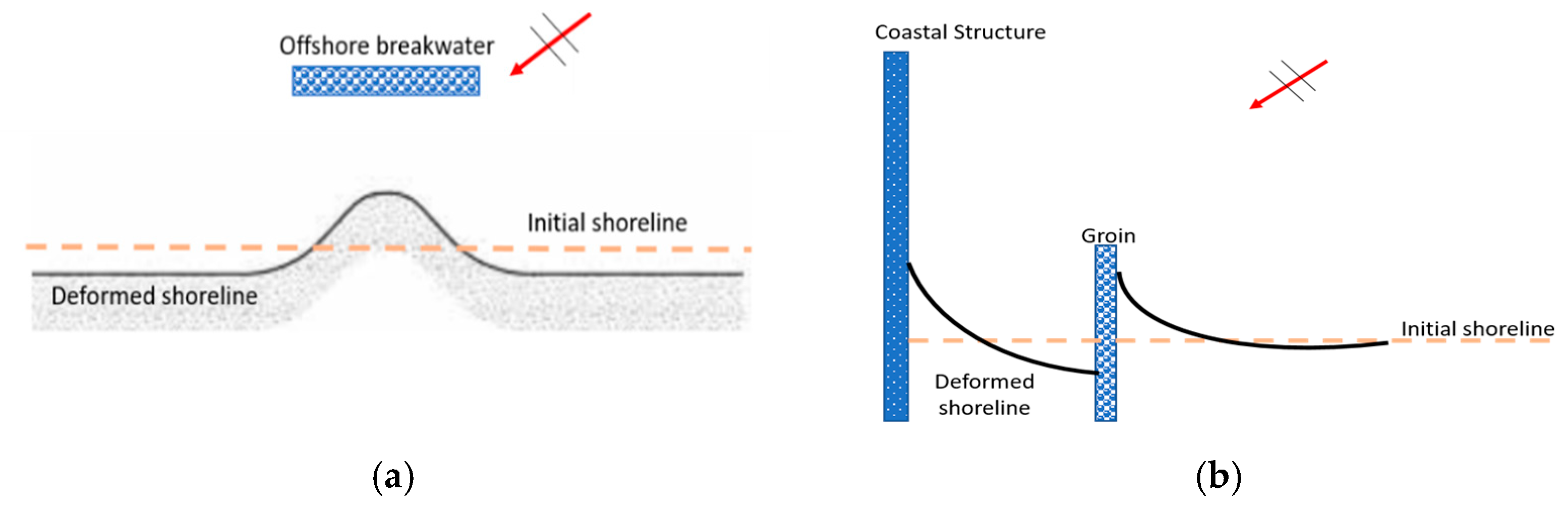
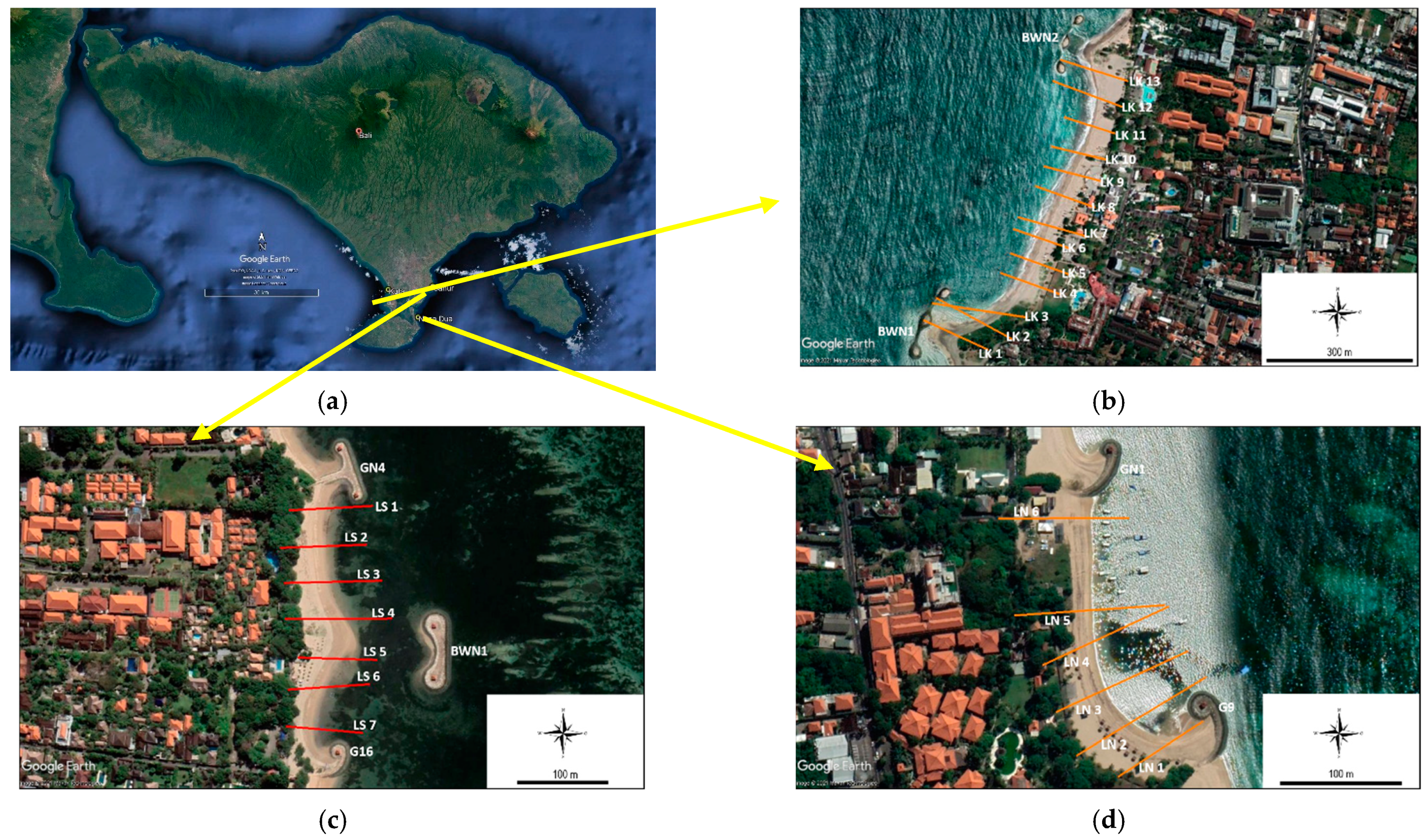
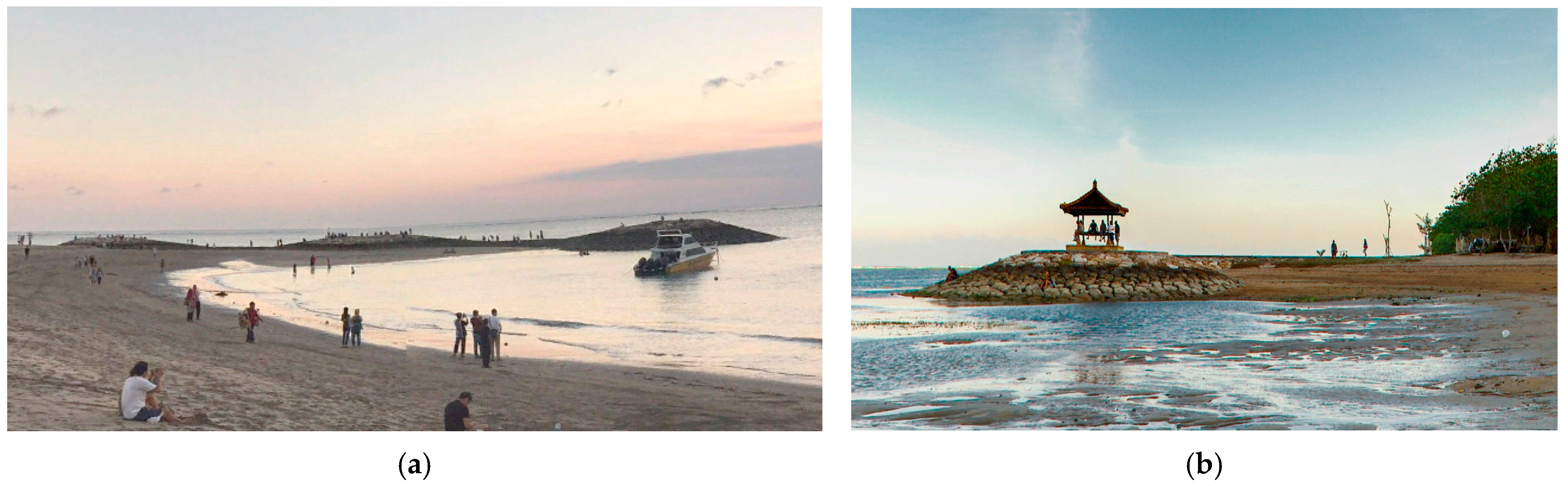
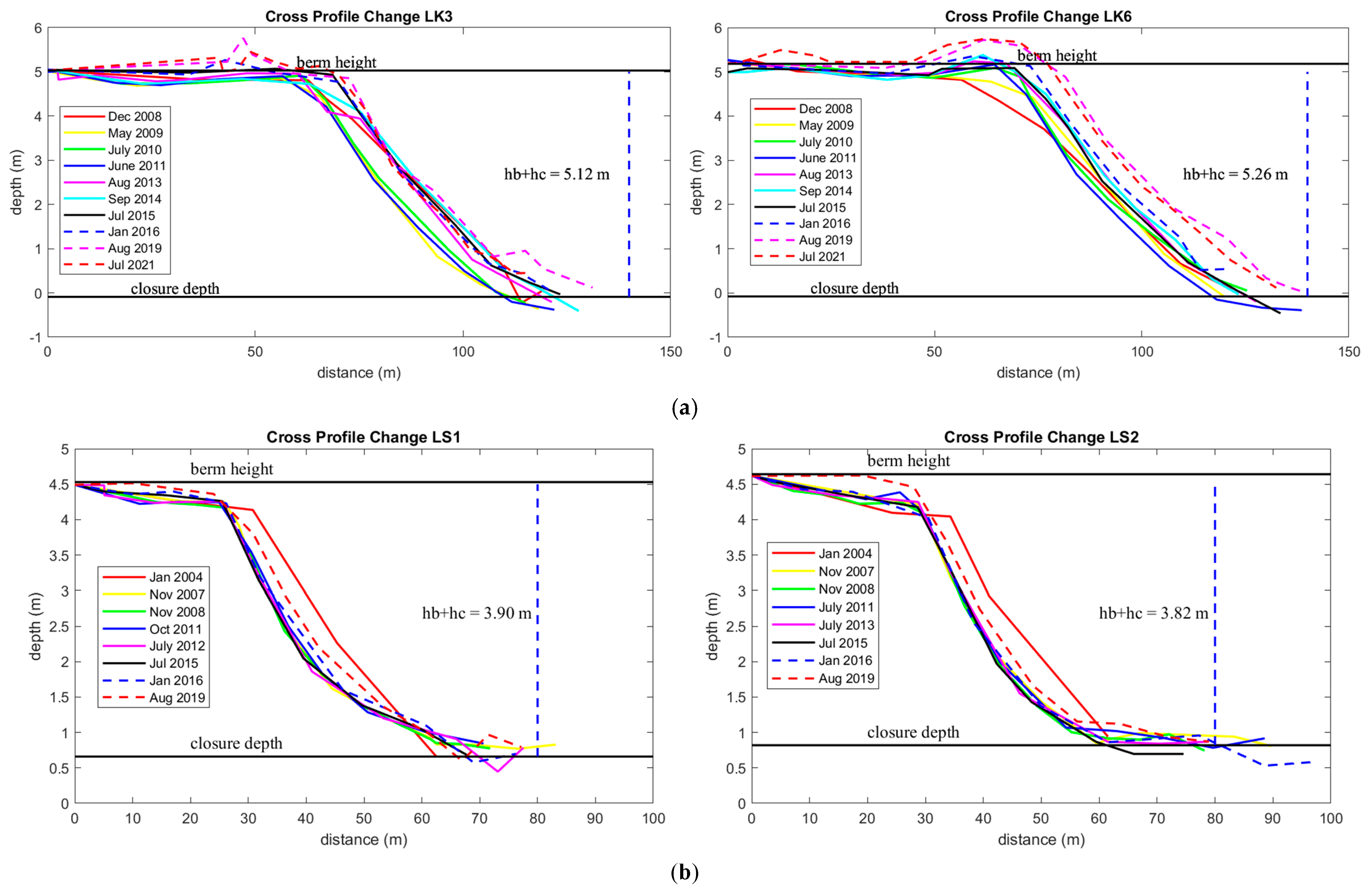
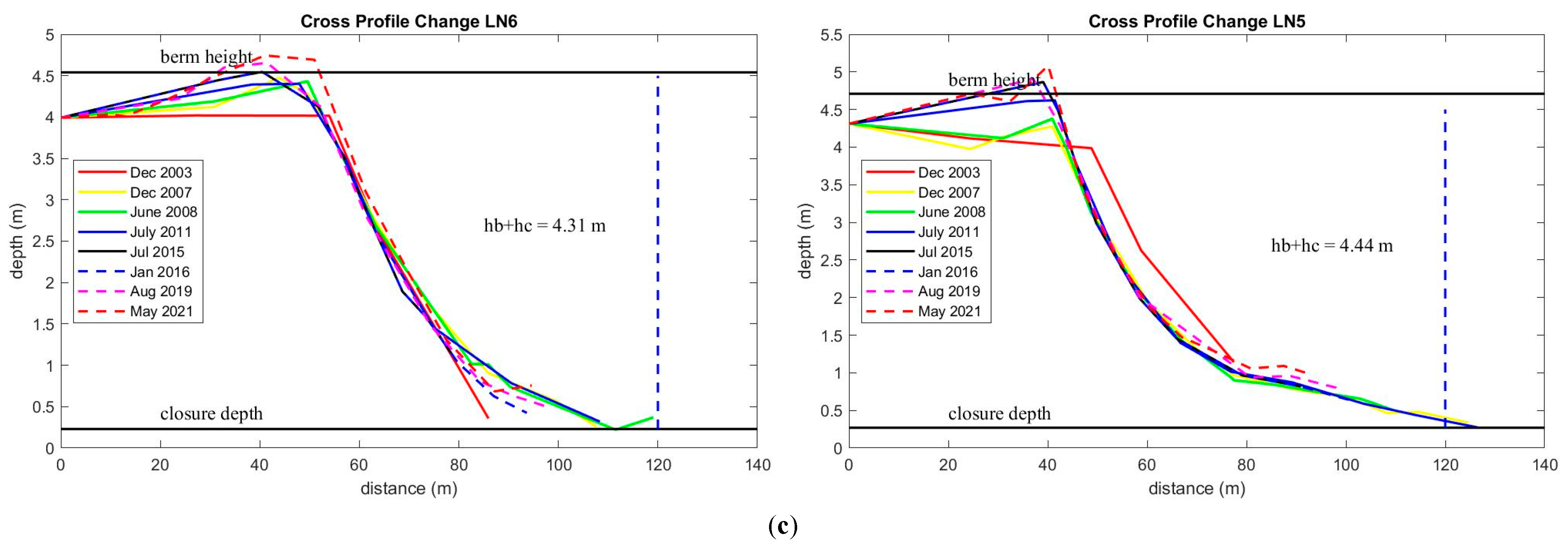
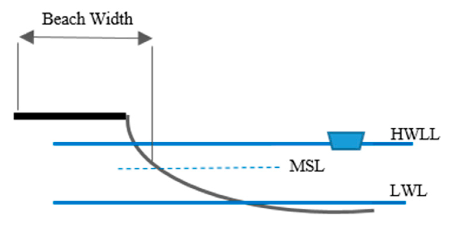
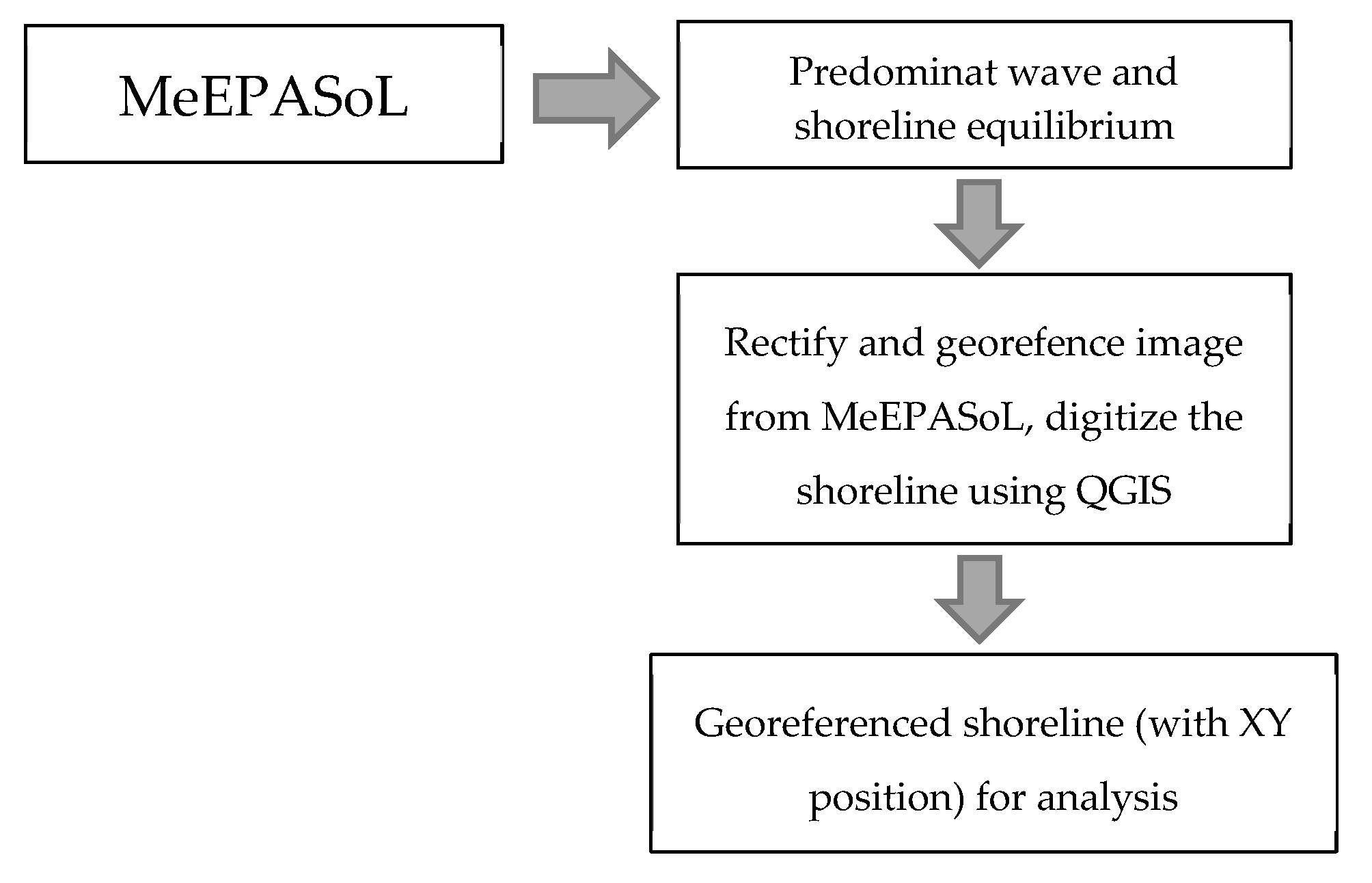
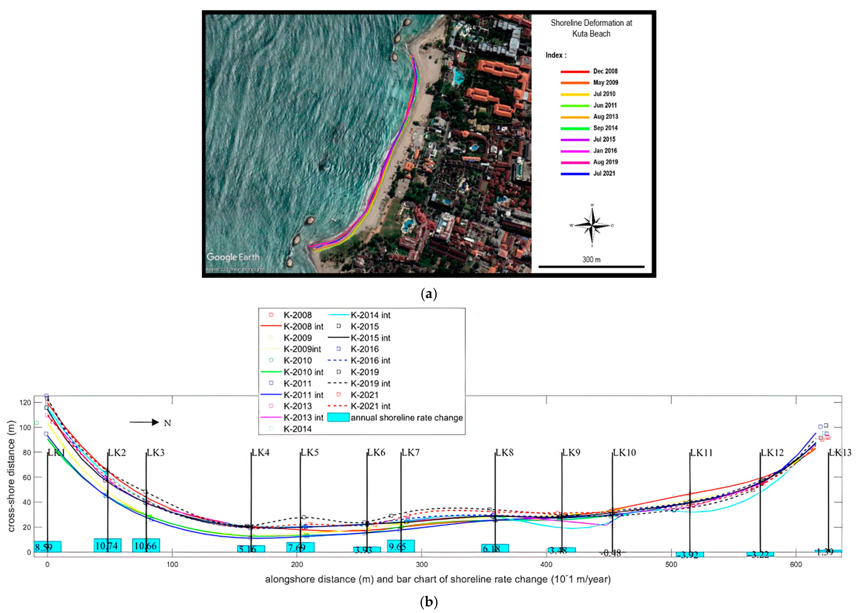
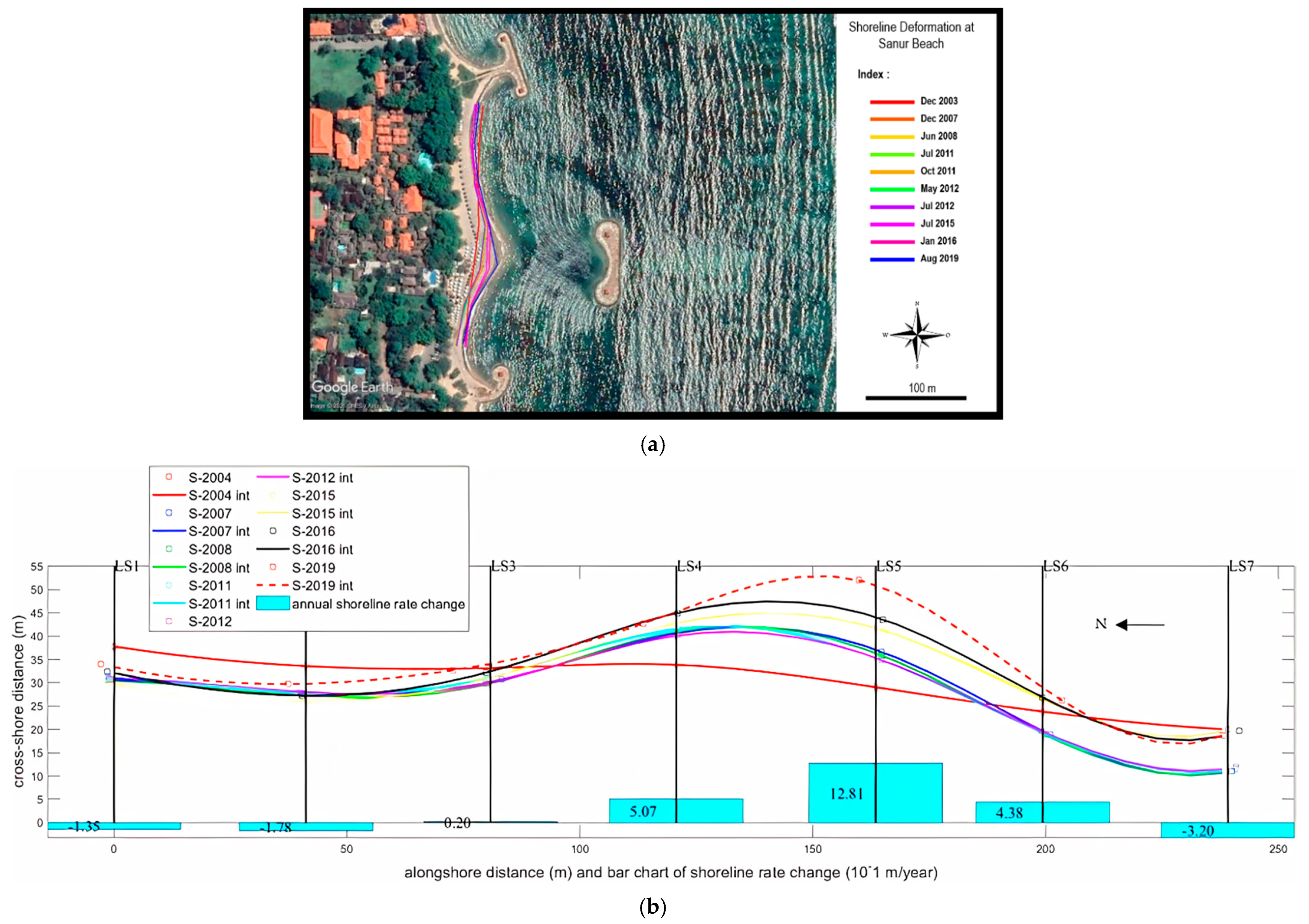
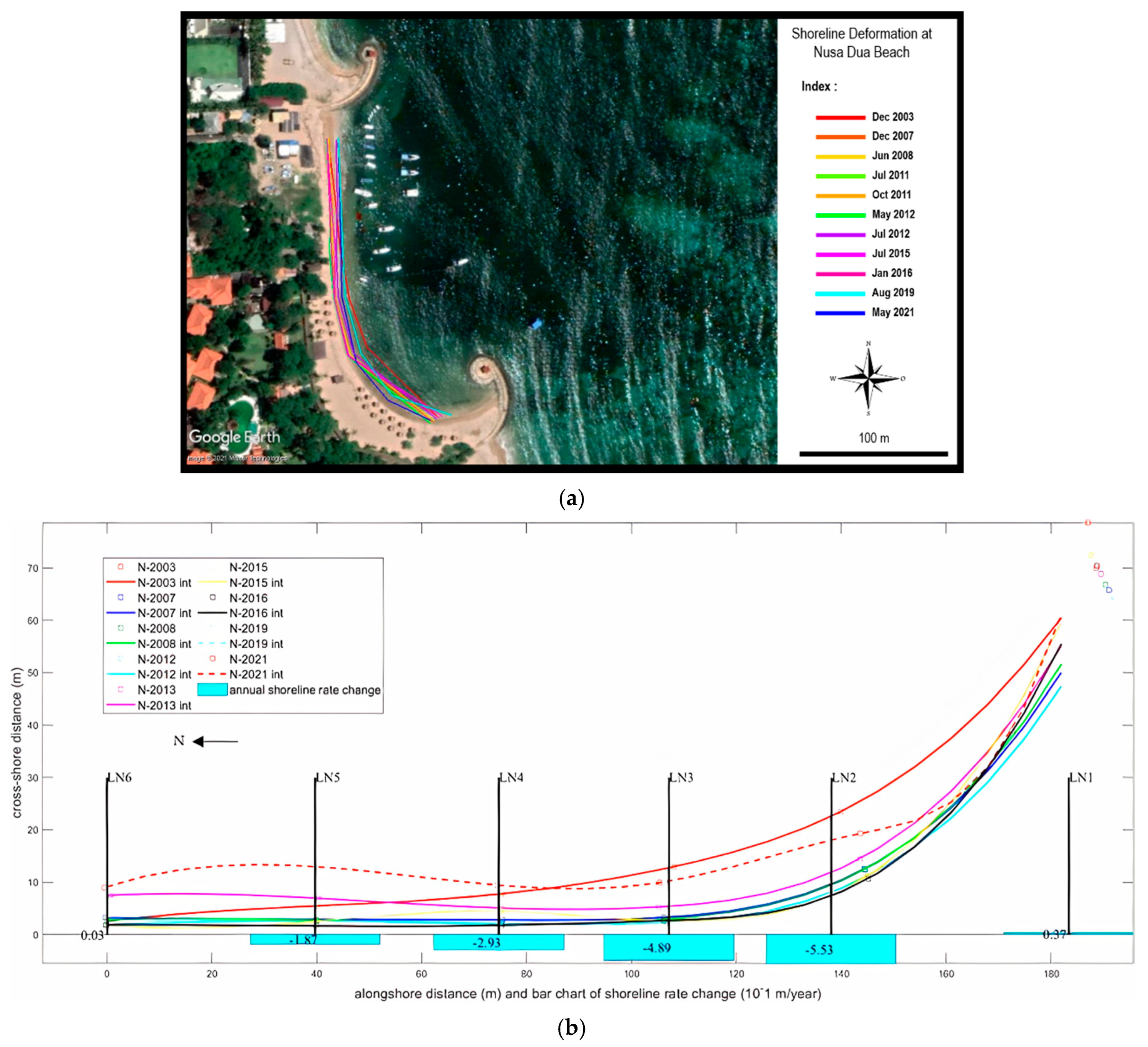
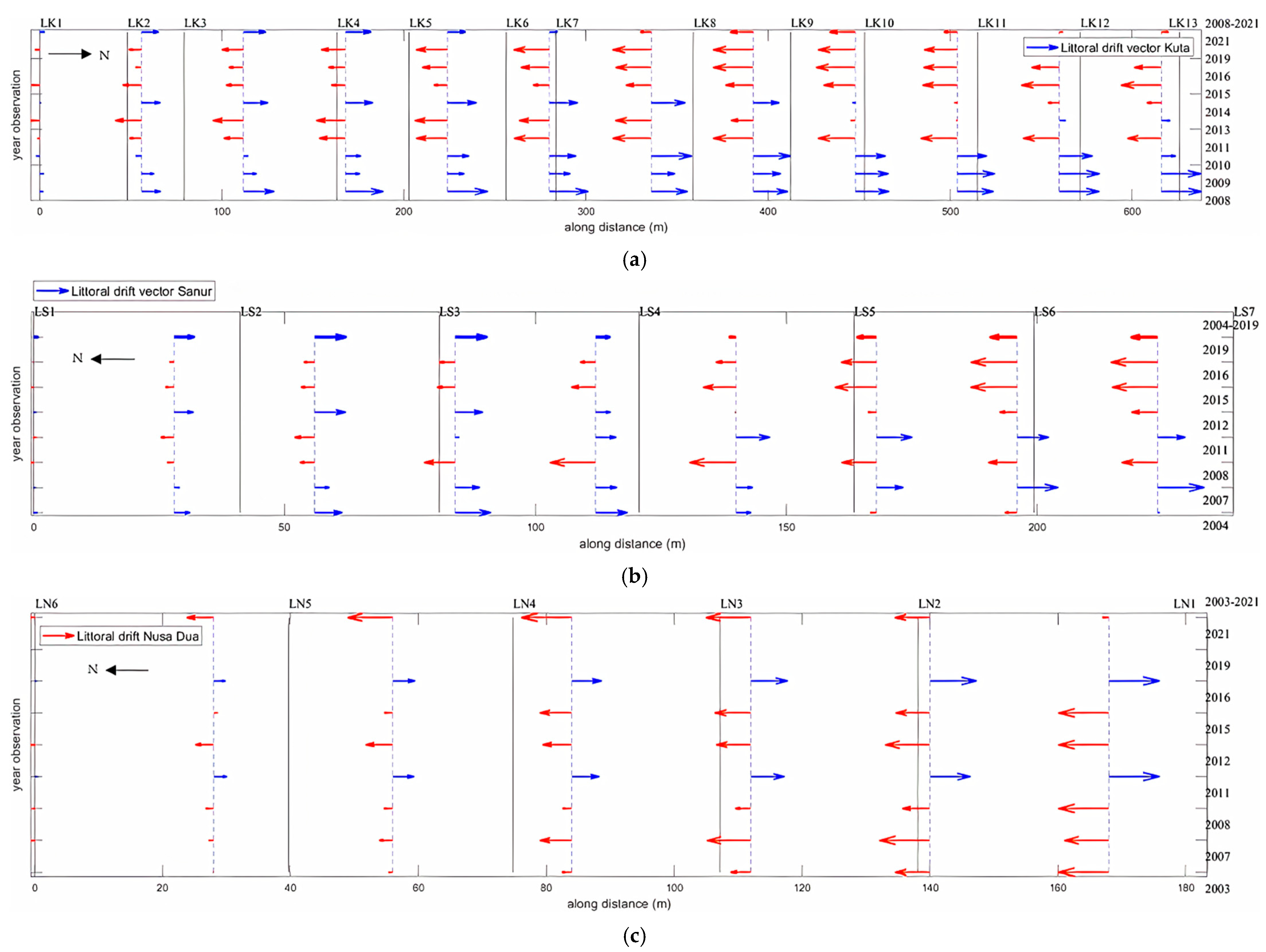
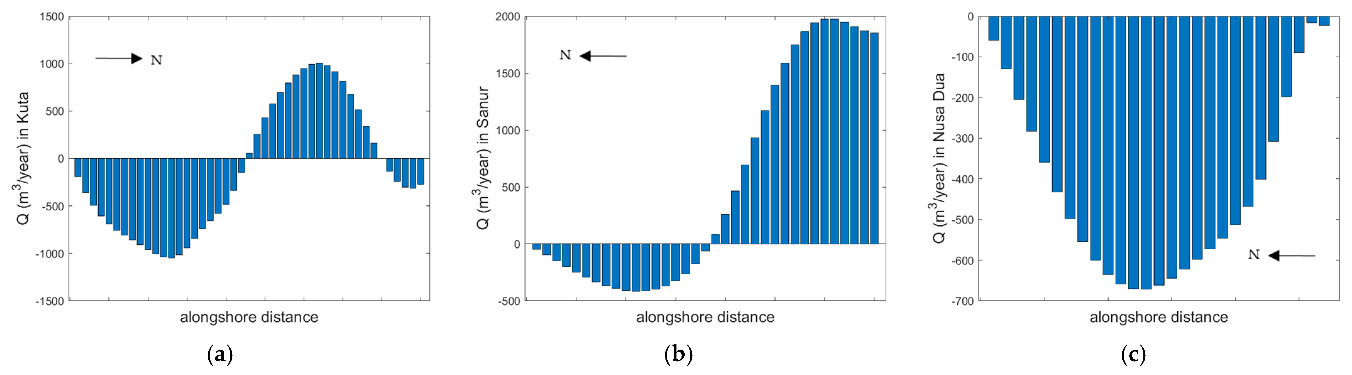
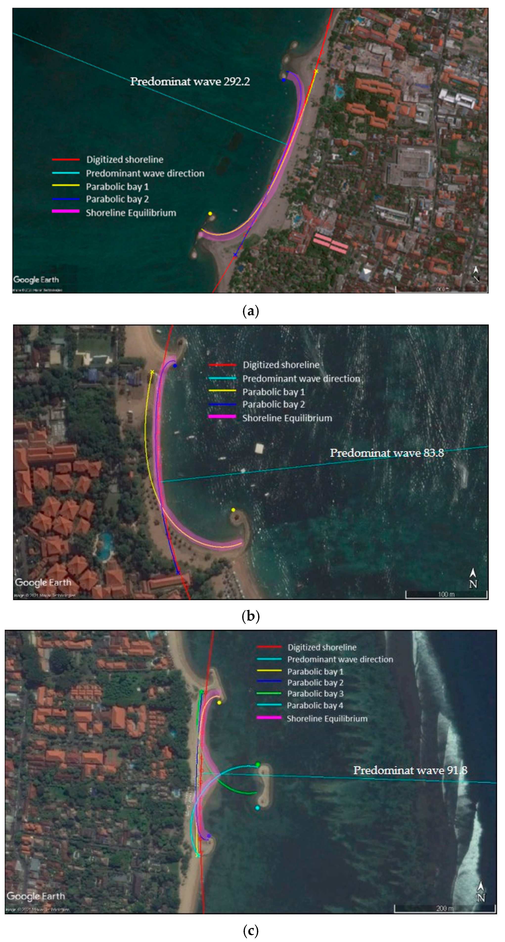
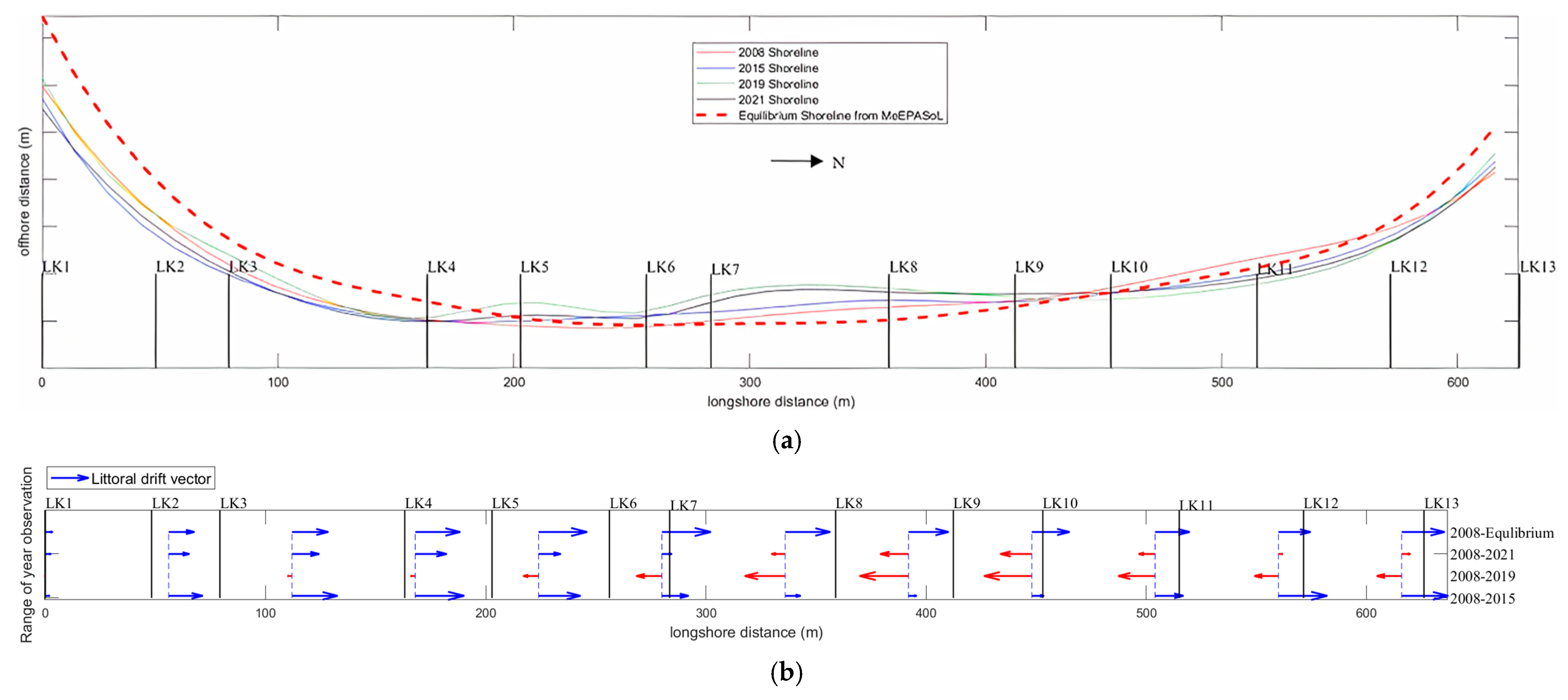
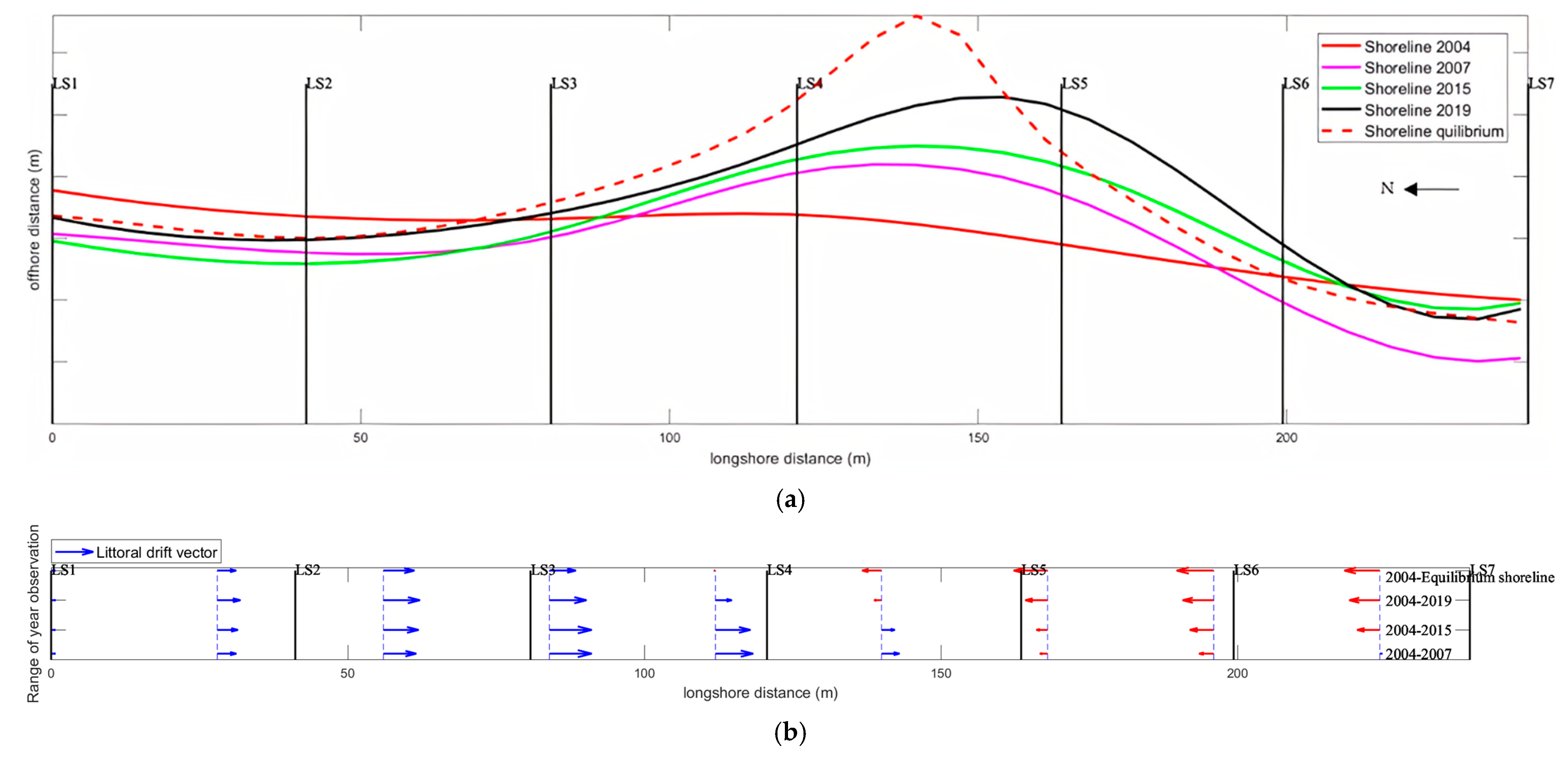
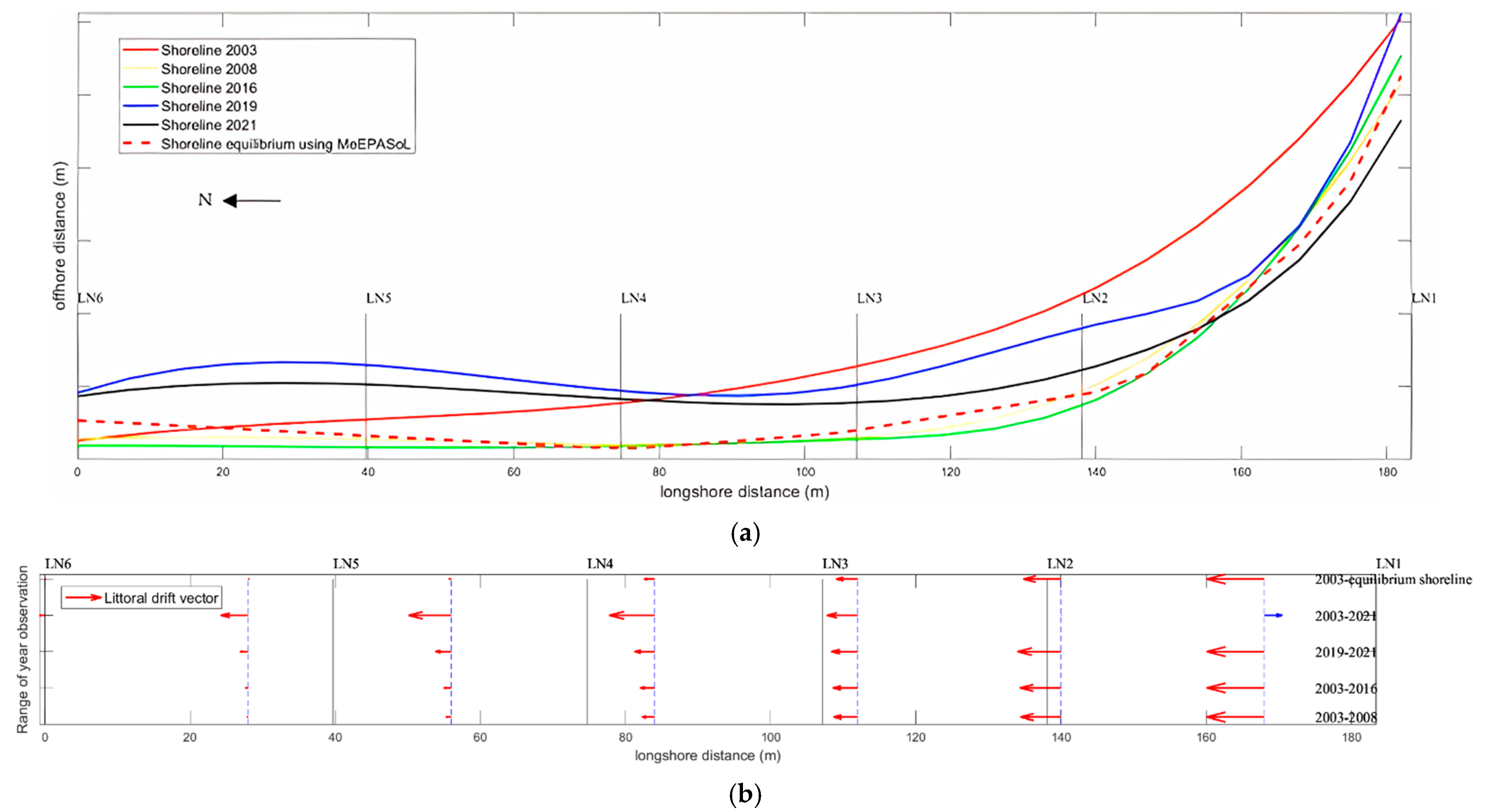
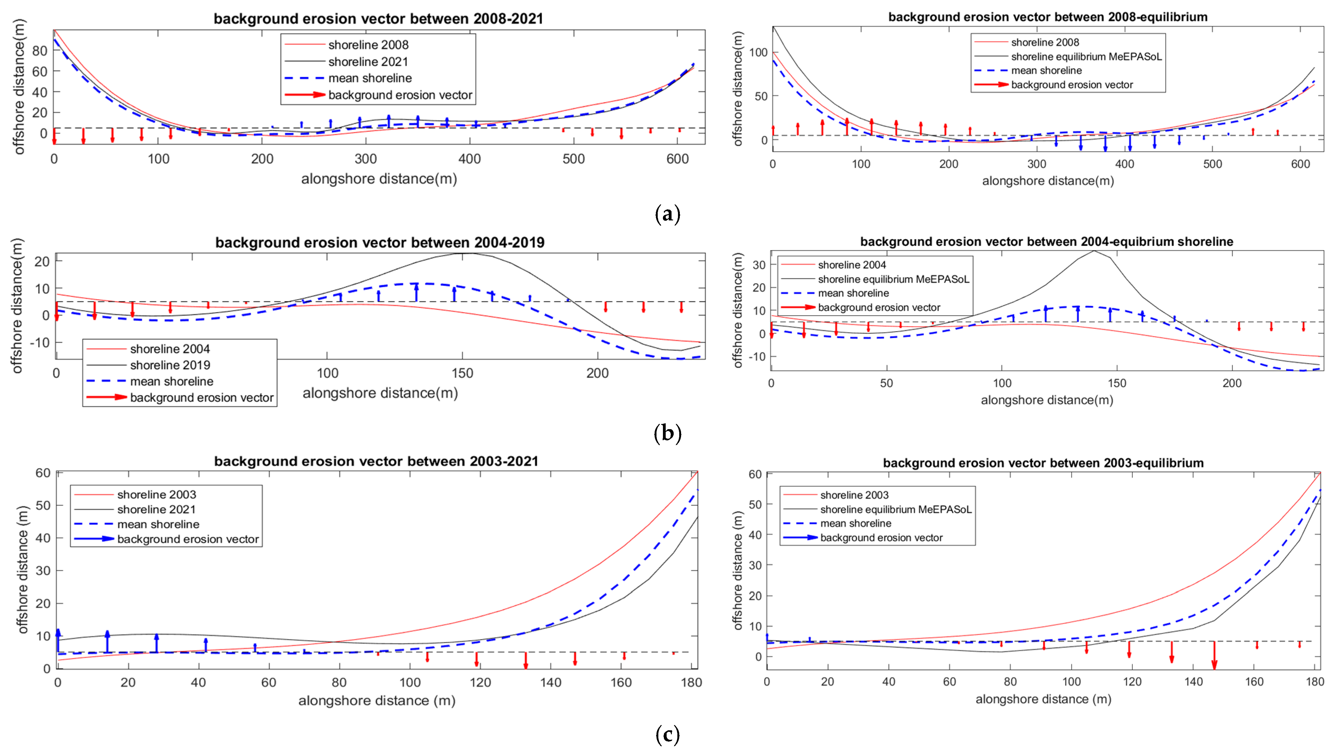
Table 1.
Study area characteristics.
| Beach | Hs (m) 1 | Ts (s) 1 | D50 (mm) 1 | Beach Nourishment (×1000 m3) 2 |
|---|---|---|---|---|
| Kuta: Kuta Beach | 1.1–2.8 | 4–8 s | 0.201 | 520 |
| Sanur: Karang Beach | 1.7–5.5 | 5–16 s | 0.606 | 300 |
| Nusa Dua: Samuh Beach | 1.7–5.5 | 5–16 s | 0.606 | 340 |
1 Data collected in Sanur (2004), Nusa Dua (2003), and Kuta (2008). Ts is a significant wave period, Hs is a significant wave height, and D50 is sediment grain size. 2 Along Kuta coast, Sanur coast, and Nusa Dua coast not specified for a certain beach or subcell.
Table 2.
Existing coastal structures.
| Beach | Beach Length (m) | Existing Structure | Dimension (m) |
|---|---|---|---|
| Kuta: Kuta Beach | 676 | offshore breakwater BWN 1 | L = 150 |
| offshore breakwater BWN 2 | L = 120 | ||
| reef flat restoration | - | ||
| Sanur: Karang Beach | 250 | Headland T groin G4 | L = 76.5 W = 3 |
| Headland L groin G16 | L = 71.1 W = 3 | ||
| offshore breakwater BWN 1 | L = 80 W = 7 | ||
| Nusa dua: Samuh Beach | 210 | Groin type L GN1 | L = 85 W = 3 |
| Groin type L G9 | L = 80 W = 73 |
Table 3.
Summary of data collection.
| Beach | Beach Length (m) | Cross-Line Observation | Beach Width (m) | Year Observation | Berm + Closure Depth (m) 1 |
|---|---|---|---|---|---|
| Kuta: Kuta Beach | 676 | 13 | 52 | 2008–2021 | 5 |
| Sanur: Karang Beach | 250 | 7 | 40 | 2004–2019 | 4.0 |
| Nusa Dua: Samuh Beach | 210 | 6 | 36 | 2003–2021 | 4.5 |
1 Berm height (hb) + closure depth (hc) definition based on the cross-shore profile data interpretation from beach profile data monitoring.
Table 4.
Mean beach area change.
| Beach | Area Change (m2) | Note | |
|---|---|---|---|
| Initial | Mean Area | ||
| Kuta | 48,620.68 | 47,636.62 | retreat |
| Sanur | 8406.00 | 8549.30 | advance |
| Nusa Dua | 9866.13 | 8583.09 | retreat |
Publisher’s Note: MDPI stays neutral with regard to jurisdictional claims in published maps and institutional affiliations. |
© 2021 by the authors. Licensee MDPI, Basel, Switzerland. This article is an open access article distributed under the terms and conditions of the Creative Commons Attribution (CC BY) license (https://creativecommons.org/licenses/by/4.0/).
Share and Cite
MDPI and ACS Style
Rahmawati, R.R.; Putro, A.H.S.; Lee, J.L. Analysis of Long-Term Shoreline Observations in the Vicinity of Coastal Structures: A Case Study of South Bali Beaches. Water 2021, 13, 3527. https://doi.org/10.3390/w13243527
AMA Style
Rahmawati RR, Putro AHS, Lee JL. Analysis of Long-Term Shoreline Observations in the Vicinity of Coastal Structures: A Case Study of South Bali Beaches. Water. 2021; 13(24):3527. https://doi.org/10.3390/w13243527
Chicago/Turabian StyleRahmawati, Ria Rista, Anthony Harlly Sasono Putro, and Jung Lyul Lee. 2021. "Analysis of Long-Term Shoreline Observations in the Vicinity of Coastal Structures: A Case Study of South Bali Beaches" Water 13, no. 24: 3527. https://doi.org/10.3390/w13243527
Note that from the first issue of 2016, this journal uses article numbers instead of page numbers. See further details here.