Article

Modelling Snowmelt Runoff from Tropical Andean Glaciers under Climate Change Scenarios in the Santa River Sub-Basin (Peru)

1
Programa de Doctorado en Recursos Hídricos (PDRH), Universidad Nacional Agraria La Molina, Ave. La Molina, S.N., Lima 15012, Peru
2
Facultad de Ciencias Agrarias, Universidad Nacional del Altiplano de Puno, Puno 21001, Peru
3
Dirección de Desarrollo Tecnológico Agrario, Instituto Nacional de Innovación Agraria, Ave. La Molina, 1981, Lima 15024, Peru
4
Instituto de Investigación para el Desarrollo Sustentable de Ceja de Selva (INDES-CES), Universidad Nacional Toribio Rodríguez de Mendoza de Amazonas (UNTRM), Chachapoyas 01001, Peru
5
Departamento de Biología, Área de Botánica, Universidad Autónoma de Madrid, Calle Darwin 2, ES-28049 Madrid, Spain
*
Authors to whom correspondence should be addressed.
Water 2021, 13(24), 3535; https://doi.org/10.3390/w13243535
Submission received: 16 November 2021 / Revised: 5 December 2021 / Accepted: 8 December 2021 / Published: 10 December 2021
(This article belongs to the Section Hydrology)

Abstract

:
Effects of climate change have led to a reduction in precipitation and an increase in temperature across several areas of the world. This has resulted in a sharp decline of glaciers and an increase in surface runoff in watersheds due to snowmelt. This situation requires a better understanding to improve the management of water resources in settled areas downstream of glaciers. In this study, the snowmelt runoff model (SRM) was applied in combination with snow-covered area information (SCA), precipitation, and temperature climatic data to model snowmelt runoff in the Santa River sub-basin (Peru). The procedure consisted of calibrating and validating the SRM model for 2005–2009 using the SRTM digital elevation model (DEM), observed temperature, precipitation and SAC data. Then, the SRM was applied to project future runoff in the sub-basin under the climate change scenarios RCP 4.5 and RCP 8.5. SRM patterns show consistent results; runoff decreases in the summer months and increases the rest of the year. The runoff projection under climate change scenarios shows a substantial increase from January to May, reporting the highest increases in March and April, and the lowest records from June to August. The SRM demonstrated consistent projections for the simulation of historical flows in tropical Andean glaciers.

1. Introduction

Global temperature has increased 0.89 °C since 1901, which has negatively affected the spatial and temporal patterns of precipitation [1]. Global warming is expected to affect river flow and increase the melting of glaciers in the coldest parts [2,3]. Ninety-nine percent of the planet’s tropical glaciers are located in the South American Andes [4]. These glaciers are the natural water storage for downstream populations in high mountain watersheds [5]. However, glacier melting affects human populations, changes the hydrological cycle, increases sea level and natural hazards [6]. Besides being an important cause of the change in glacier morphology, it can provide basic parameters for assessing water resources [7]. This retreat of glaciers and snow is threatening the sustainability of water resources in mountainous regions, which means that watersheds are constantly exposed to variations caused by climate change [8]. Therefore, it is necessary to accurately simulate and forecast snowmelt runoff in the different high Andean regions.
In the last decades, many models have been constructed to estimate or forecast snowmelt runoff under different hydrologic conditions [9]. These can be generally classified as empirical temperature index (TI) models employing a degree-day orientation or energy balance (EB) model with a physically based approach in which the various heat fluxes at the snow or ice surface are quantified [10,11]. The EB model requires a lot of data and vertical gradients of specific temperature and humidity, wind speed, incoming radiation and precipitation [12]. However, degree-day models have been developed in response to the high requirements of the EB model, as they allow temperature to be used as a relatively accurate index for estimating ice-melt mass [13,14]. Other models, such as the Water Evaluation And Planning (WEAP) system, have been applied to assess the water management implications of a possible future glacier retreat. [15,16].
Remote sensing is an important tool in capturing spatial information on hydrological state and flow variables such as precipitation, snow cover area (SCA), snow water equivalent (SWE) and total water storage change (TWS), as well as land surface properties (land surface temperature—LST, and land surface albedo) that are important for improving predictions in hydrological modelling in high mountain regions [17,18]. The spatial and temporal resolutions of images for snowmelt runoff modelling are defined by the size of the watershed or study area [19]. Thus, in the last 20 years, there has been an increase in the availability of snow products, which are available for use at different spatial resolutions, from sensors such as the Advanced Very High Resolution Radiometer (AVHRR), the Special Sensor Microwave Imager (SSMI), the Advanced Microwave Scanning Radiometer-Earth Observing System (AMSR-E) and the Moderate Resolution Imaging Spectroradiometer (MODIS) and Landsat Instruments [10]. The snowmelt runoff model (SRM), on the other hand, is a conceptual hydrological model for simulating runoff in snowmelt-dominated watersheds that incorporates remotely sensed imagery and requires three input variables: temperature, precipitation, and SCA [13,20].
In recent years, snow cover maps obtained from MODIS represent valuable information due to their high temporal (1 day) and spatial resolution (500 m) [21]. However, the precision is influenced by environmental conditions, land use (presence of forested areas) and accumulation of shallow or irregular snow [22,23,24]. Studies show that the combination of Terra and Aqua MODIS images can improve the overall accuracy of SCA prediction in open areas and alpine and forested regions by using the Generalized Probability Uncertainty (GLUE) estimation methodology, in situ measurements of snow depth (SD) and snow water equivalent (SWE), in situ snow cover telemetry (SNOTEL) [21,24,25,26].
In Peru, the Cordillera Blanca (CB) hosts some of the most important glaciers, located in the Andes western branch, it is the highest and most extensive tropical glacier in the world and represents approximately 35% of the glacier area of Peru [27,28]. These are temporary water storages in snow that form at high altitudes during the rainy season, between October and April [29]. They release water in the dry season (May and September) that flows through the Santa river valley and is used for human consumption and in activities like mining, agriculture and power generation [30,31]. From 1930 to 2014, glaciers in this region were reduced by more than 30% of their surface area and, currently, this dynamic continues [29]. Should this situation continue, there would be a shortage of water for the consumption of rural and urban communities settled along its watersheds [32]. On the other hand, in the BC, the existence of 755 glaciers with a surface area of 527.62 km2 has been reported that are confined to mountain slopes and generally located on slopes greater than 25% of inclination [33]. Likewise, the mass balance variations in BC show that it responds to fluctuations in climate (temperature, humidity and precipitation) on a large scale, dominated by conditions in the tropical Pacific. The ENSO is the main pacemaker on interannual time scales causing positive mass balance anomalies during La Niña and negative anomalies during El Niño events [34,35]. Here lies the importance of knowing the response of glaciers to climate change.
The objective of this study was to apply the SRM in concert with information SCA and climatic data of temperature and precipitation to model melt runoff in the Santa river sub-basin (Peru). In sum, we (i) determined the SCA trend, using remote sensing techniques and the Google Earth Engine (GEE) platform, and (ii) modelled snowmelt runoff under climate change scenarios for 2030, 2050 and 2080.

2. Materials and Methods
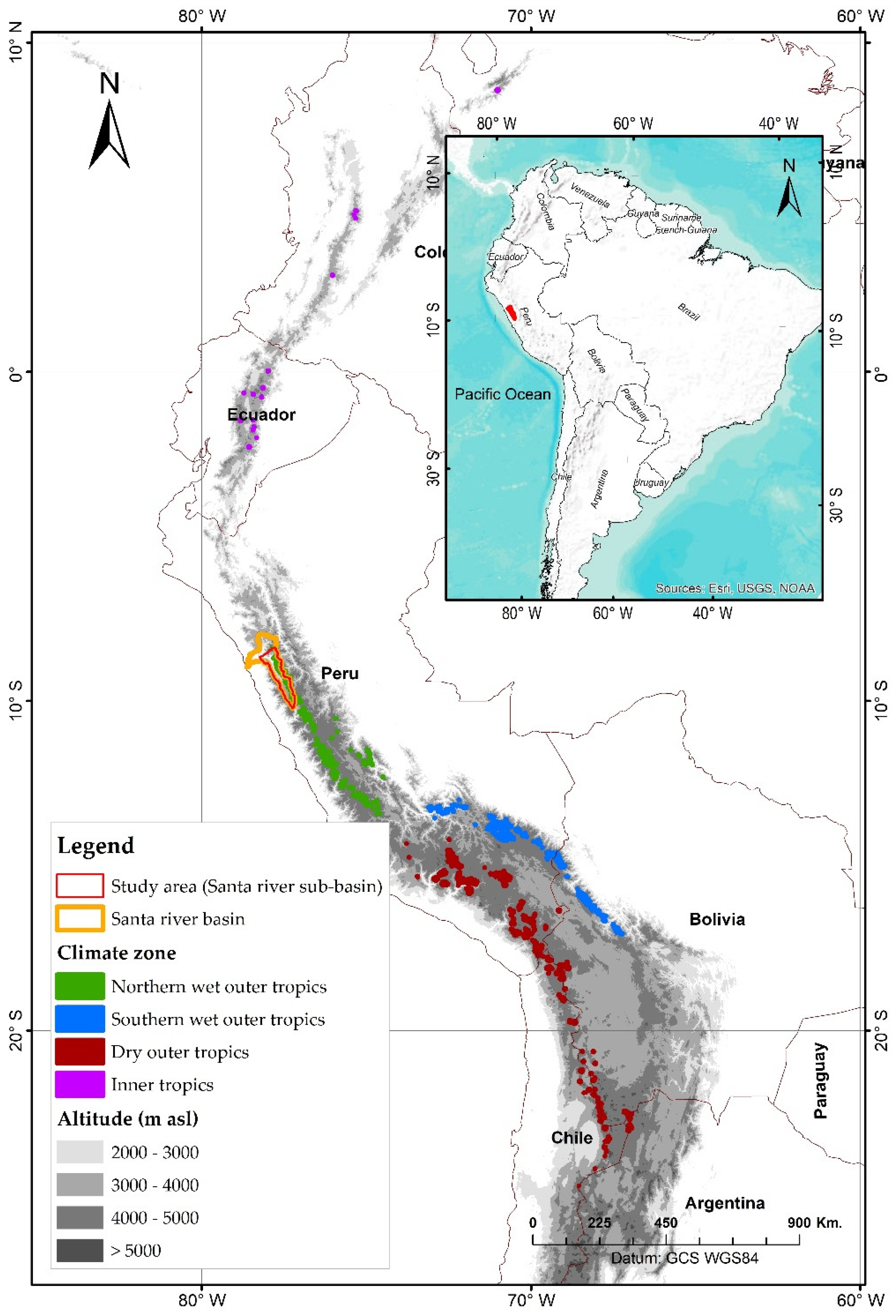
2.1. Study Area

The Santa River sub-basin is part of the basin of the same name. It is located in the Tropical Andes and includes the western flank of the BC (Figure 1). Politically, it is located between the departments of Ancash and Trujillo, belonging to the highland region of Peru. It runs into the western part of the BC and in turn separates it from the Cordillera Negra in the west. It is characterized by a mixed hydrological regime with two well-defined seasons during the year: the wet season from October to April [29] and the dry season from May to September [30]. From a glaciological point of view, it is located in the humid northern outer tropics [4] with a total area of 5334 km2 and average altitudinal gradient of 4087 m, a humid and very cold climate predominates with annual maximum temperatures between 18 to 24 °C, and minimum temperatures between 16 and −4 °C. Precipitation increases from west to east, accumulating more than 500 mm per year in areas above 2500 m and rainfall of greater intensity in the northern border area exceeding 3500 m. In the southeast of the sub-basin, annual precipitation ranges from 400 to 1200 mm per year.
The water of the Santa River depends on glacial and non-glacial sources and is vital for the population settled in the area of the sub-basin (453,950 inhabitants) and the development of economic activities [15,36,37]. Among the main activities that take place above 5000 m, the glaciers and mountain tops themselves are a tourist attraction around the world, between 2000 and 4000 m Quechua farmers develop hillside agriculture and below 2000 m. The extraordinary natural landscape of the Pato Canyon is used, a hydroelectric project is developed, and the water is used to irrigate huge agricultural areas [15,32,37]. However, water resource use conflicts have been reported among nearby communities in the departments of Ancash and La Libertad, arising from changes in water availability as a result of climate variability, socioeconomic factors and mining activities [38]. This could have an impact on the food security of settlements that depends directly on this resource.

2.2. Data Processing

Figure 2 shows data processing for modelling snowmelt runoff from tropical Andean glaciers under climate change scenarios in the Santa river sub-basin. Briefly, observed climate data of temperature, precipitation, digital elevation model (DEM) and MODIS images were acquired to estimate the SCA [39]. Subsequently, the SRM model was applied to simulate the surface runoff of the sub-basin. Finally, the model was validated and calibrated to obtain future runoff scenarios under a climate change context.

2.3. Historical Climate and Discharge Data

Daily climatic data for temperature and precipitation were downloaded from the Servicio Nacional de Meteorologia e Hidrologia (SENAMHI) and the Unidad de Glaciologia y Recursos Hídricos (UGRH)—Huaraz from the meteorological stations of Yungay (2496 m), Recuay (3431 m), Yanamarey (4606 m) and Artesonraju AP2 (4834 m) between 2000 and 2017 (Table S1). Daily flow data were collected between the period 2000 to 2009 from the hydrometric stations La Balsa, Quitarcsa and Los Cedros. Likewise, the temperature variation ratio per 100 m was determined, comparing the temperature variation in three representative meteorological stations in the study area. Which was used to adjust the height ∆T (Equation (1)) in the six hypsometric zones [20].
∆T = γ × (hst − h) × 1/100
where: γ = Rate of temperature variation [°C every 100 m], hst = Altitude of the station where the temperature is measured.
The average of the temperature variation ratio of three stations (Yungay, Recuay and AP2) was used, which was 0.55, used for the correction of the temperature variable in the six hypsometric zones. For the precipitation input data, they were extrapolated according to the mean hypsometric height of each zone with an increase of 3% to 4% of precipitation per 100 m as recommended by Martinec et al. [20].

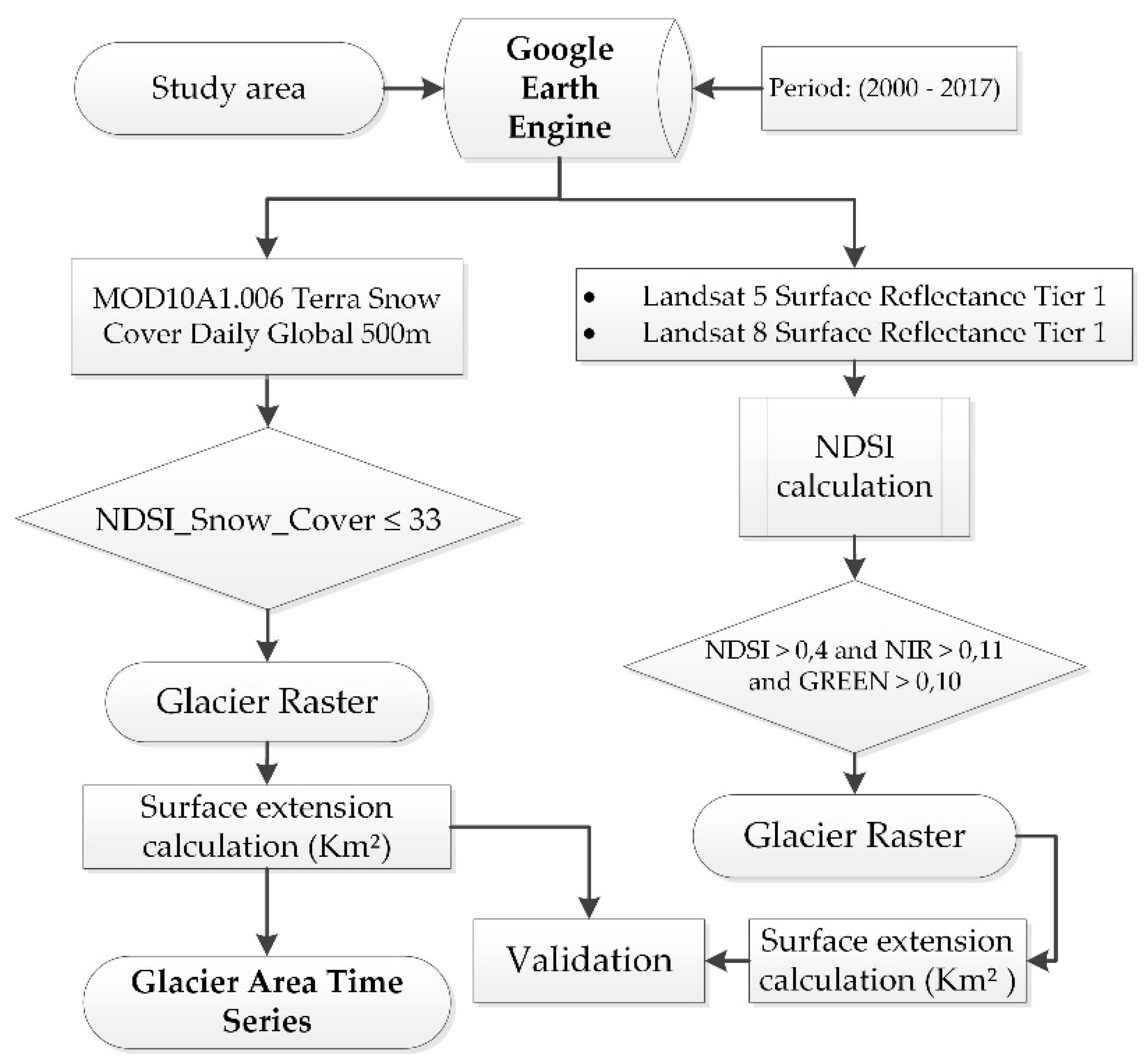
2.4. Estimation of Snow Covered Area (SCA)

The SCA estimation was performed based on the MODIS Snow Cover MOD10A1 product with daily temporal resolution and 500 m spatial resolution [40]. All images from the period 2000 to 2017 [40,41] were processed using the GEE platform [42]. For SCA validation, Landsat 5 (Surface Reflectance Tier 1) and Landsat 8 (Surface Reflectance Tier 1) images were used by determining the Normalized Difference Snow Index (NDSI), as proposed by Riggs et al. [43]. The process consisted of classifying Landsat images into glacier and non-glacier [44]. Finally, the Terra and Aqua satellite MOD10A1 product was validated (Figure 3).

2.5. Snowmelt Runoff Model (SRM)

The SRM is a semi-distributed model based on the degree-day factor that has been applied in several high mountain basins with different areas and altitudinal ranges [20]. The degree-day approach has been particularly interesting for snow hydrology research in regions with sparse meteorological networks and limited capacity for field measurements needed to physically calibrate the model [45,46,47]. The DSM was reclassified into six zones as proposed by Martinec et al. [20] to estimate the SCA of each altitudinal zone and generate the sub-basin hypsometric curve.
The daily input data used in the SRM were temperature, precipitation and SCA. Additionally, the model considered some sub-basin characteristics such as location, elevation and hypsometric curve. The record register date from 2000–2017 was used for the statistical analysis of correlation between these variables, and from 2005 to 2008 for the simulation and validation of the SRM, which was run on the WinSRM software. The model also calculated the daily amount of water from snowmelt and rainfall; this amount is added to the recession flow to obtain the total daily flow according to Equation (2) [20].
Q n + 1 = [ c s n ] a n ( T n + Δ T ) S n + c R n P n A 10000 86400 ( 1 k n + 1 ) + Q n k n + 1
where Q is the average daily discharge (m3 s−1), C runoff coefficient, expressing the losses as a ratio (runoff/precipitation), C s the snowmelt C r rainfall, a degree-day factor (cm °C−1 d−1), indicating the snowmelt depth resulting from 1 degree-day, T number of degree-days (°C d), Δ T the adjustment by temperature lapse rate when extrapolating the temperature to the average hypsometric elevation of the basin or zone (°C d). S , ratio of the snow-covered area to the total area. P, precipitation contributing to runoff (cm). T c r i t critical temperature, determines whether this contribution is rainfall and immediate. If precipitation is determined by Tcrit to be new snow, it is kept on storage over the hitherto snow free area until melting conditions occur, A area of the basin (km2). K recession coefficient indicating the decline of discharge in a period without snowmelt or rainfall, where K = Q m + 1 / Q m , (m, m + 1 are the sequence of days during a true recession flow period) and n sequence of days during the discharge computation period.
T , S and P are variables to be measured or determined each day. C s , C r , lapse rate to determine Δ T , T c r i t , k and the lag time are parameters which are characteristics for a given basin or, more generally, for a given climate. For this study, the sub-basin was divided into six zones, 900 m approximately, following Equation (3).
Q n + 1 = [ c S A n ] a A n ( T n + Δ T A n ) S A n + c R A n P A n A A 10000 86400 + [ c S B n ] a B n ( T n + Δ T B n ) S B n + c R B n P B n A B 10000 86400 + [ c S C n ] a C n ( T n + Δ T C n ) S C n + c R C n P C n A C 10000 86400 + [ c S D n ] a D n ( T n + Δ T D n ) S D n + c R D n P D n A D 10000 86400 + [ c S E n ] a E n ( T n + Δ T E n ) S E n + c R E n P E n A E 10000 86400 + [ c S E n ] a E n ( T n + Δ T E n ) S E n + c R E n P E n A E 10000 84400 + ( 1 k n + 1 ) + Q n k n + 1 a

2.6. SRM Model Calibration

The WinSRM was used to graphically compare the computed model with the hydrograph model. In the first stage, a visual inspection analysing the accuracy of the simulation was done. In the second stage, a statistical analysis was carried out using accuracy criteria such as the Nash-Sutcliffe correlation of the R2 coefficient of determination (Equation (4)), and the volume difference Dv: (Equation (5)), to obtain an accurate and objective evaluation of the simulation.
R 2 = 1 i = 1 n ( Q t Q t ) 2 i = 1 n ( Q t Q ¯ ) 2
where: R 2 : A measure of model efficiency, Qt: Measured daily discharge (m3/s), Q t :   Simulated daily discharge (m3/s), Q ¯ :   Average daily discharge for the simulation season (m3/s) and n: Number of daily discharge values.
D v = V R V R V R 100    
where: D v : percentage difference between the total measured and simulated runoff (%), V R : measured runoff volume (m3) and V R : simulated runoff volume (m3).
To reduce quadratic differences and the resulting sensitivity at extreme values by the NSE, the Nash-Sutcliffe coefficient was computed, using logarithmic values of the observed and simulated discharge, as a result of which the influence of low discharge rates increases the errors and makes the measurement of the statistical criterion more sensitive (Equation (6)).
R 2 = 1 i = 1 n ( log Q t log Q t ) 2 i = 1 n ( log Q t log Q ¯ ) 2

2.7. Data of Future Climate

Projected temperature and precipitation data from the general circulation model (GCM) (https://gisclimatechange.ucar.edu/, May 2018) were used for different scenarios (RCP 4.5 and RCP 8.5). Scenarios for 2030, 2050 and 2080 were analysed. The GCM climate scenario data were spatially scaled using the downscaling technique has three steps: (1) determining a simple linear model for every location in the prediction domain, (2) using an off-the-shelf method to provide an initial estimate at every prediction location from the Community Climate System Model (CCSM) data, and then (3) applying the linear model to the initial estimate to produce the final downscaled estimate, it was developed by Tim Hoar and Doug Nychka at Institute for Mathematics Applied to Geosciences (IMAGe) and National Center for Atmospheric Research (NCAR) [48].

3. Results

3.1. Snow Coverage Validation

Table 1 and Table S2 show the percentage of SCA for MODIS and Landsat data products obtained on the same overlapping date. The highest percentage of snow was reported in 2009 (6.9%), while the lowest was obtained in 2016 (4.6%) for MODIS data. However, for Landsat data, the maximum value (6.5%) was reported in 2003 and 2008, while the minimum was reached in 2015 (5.1%). Figure 4 also presents the results of the spatial distribution of the SCA for both products in 2003, 2006, 2010 and 2016.

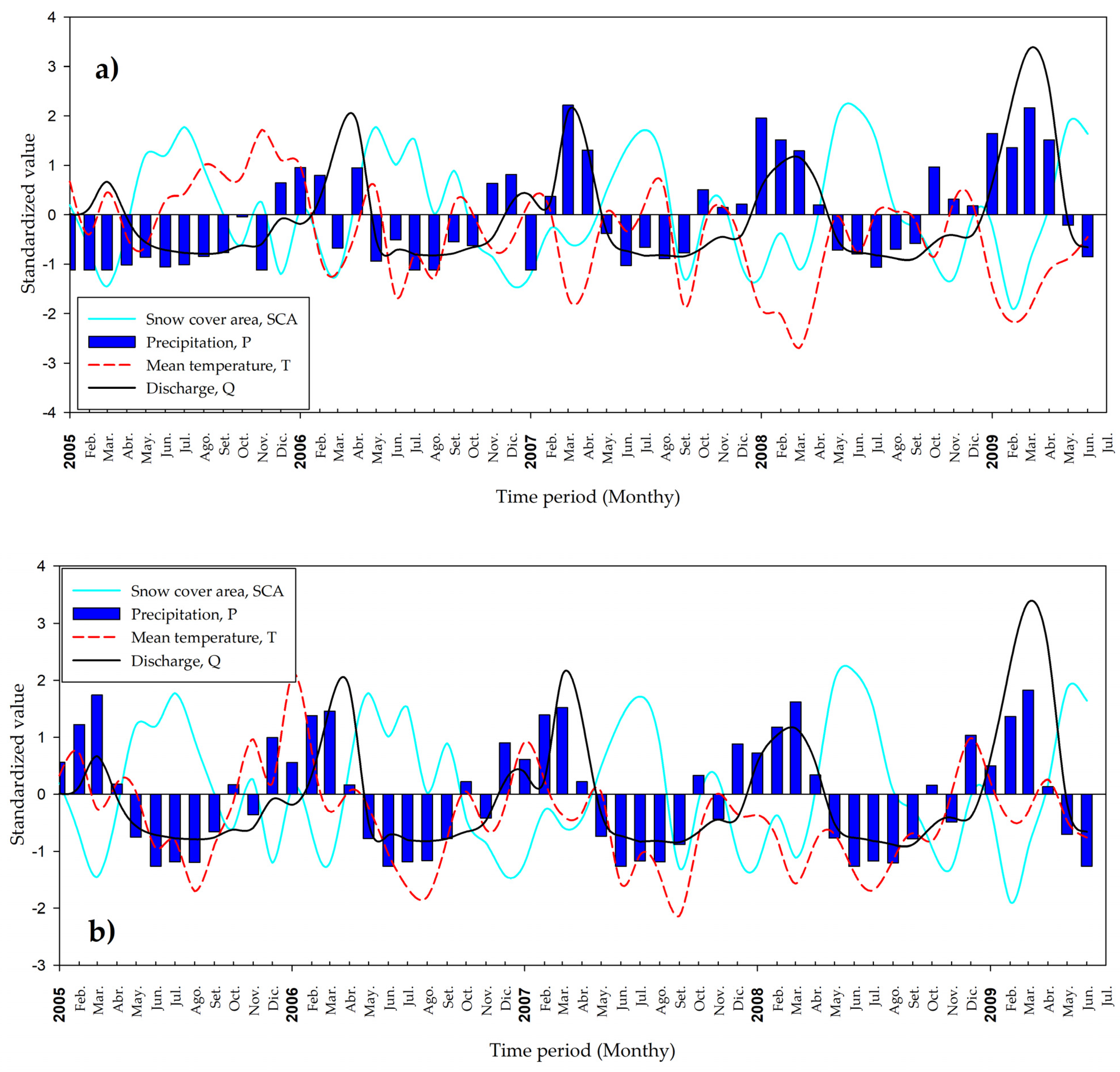
3.2. Standardised Correlation Analysis of Precipitation, Temperature, SCA and Discharge

The correlation among standardized values of precipitation, average temperature, SCA and discharge (stations of La Balsa, Quitarcsa and Los Cedros) in the Santa River sub-basin used a 5% significance level (Table S3). Figure 5 shows the standardised correlations between the input variables (precipitation, temperature, SAC and monthly discharge rate) at the Artesonraju AP2 and Yanamarey stations (over 4000 m above sea level) in the simulated period from 2005 to 2009 using SRM. It is shown that at the Yanamarey (Figure 5a) and Artesonraju AP2 (Figure 5b) stations, precipitation is an inversely proportional variable for SCA accumulation during spring and summer seasons. In turn, temperature represents an important variable in the decrease in SCA during these two seasons. Discharge increases due to the loss of ACS and precipitation events. In the drought months (autumn and winter) a different situation occurs, since temperature, precipitation and water flow decrease, presenting a positive behaviour with respect to the accumulation of SCA from the end of April to approximately September.

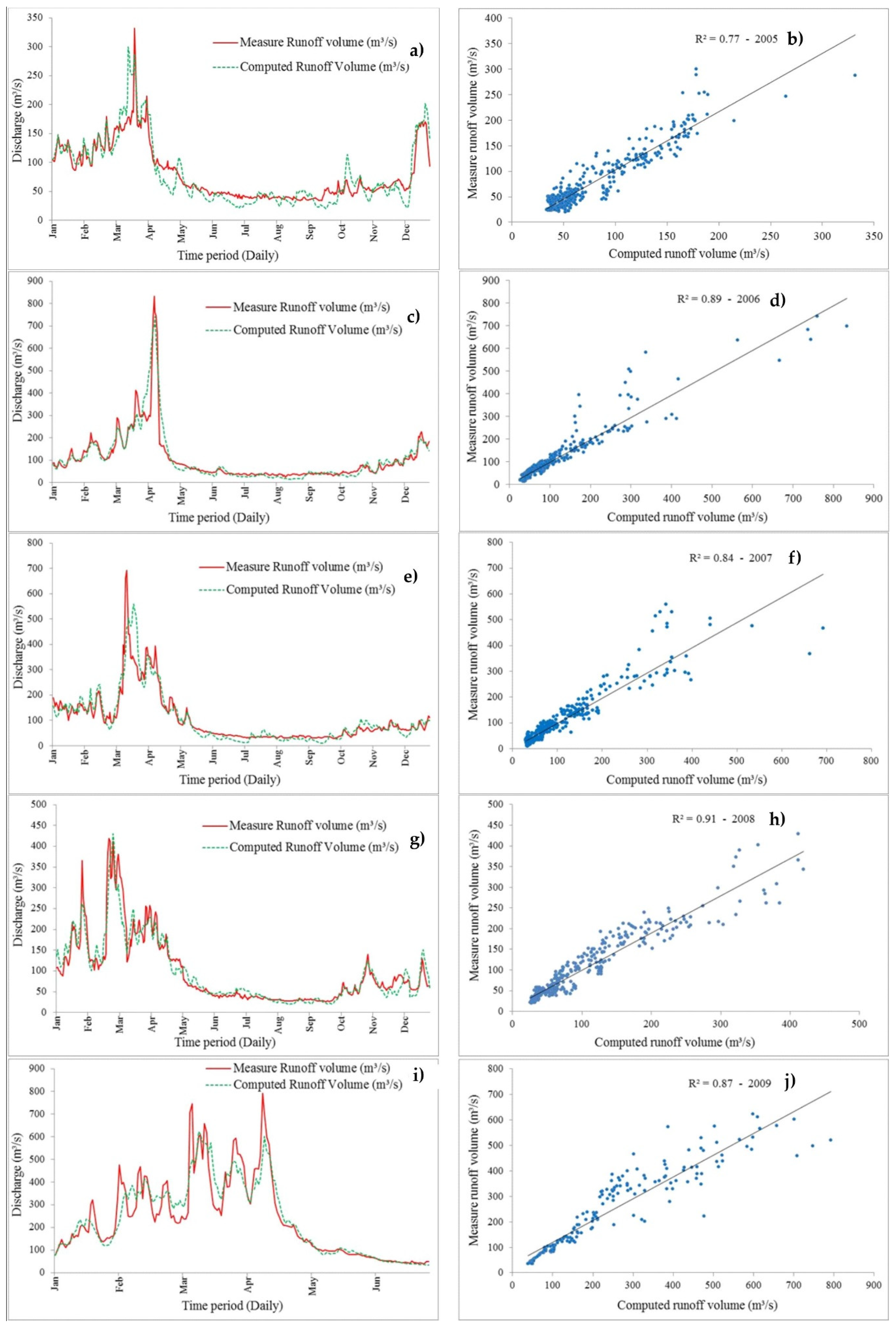
3.3. Simulation, Calibration and Validation of the SRM

Figure 6 displays the time series and scatter plots of the calibration for 2005, 2006, 2007, 2008 and 2009. Simulation for 2005 was performed using information from the observed sum at the three hydrometric stations (La Balsa, Quitarcsa and Los Cedros). In the calibration results, the Nash–Sutcliffe determination coefficient was 0.80 and Log Nash–Sutcliffe 0.67, with a volume difference of 3.95% between simulated and observed (Table 2). Highest adjusted months were from November to April, during spring and summer seasons. It reached an average discharge of 140 m3/s, due to rainfall and glacier melt (Figure 6a). In autumn and winter seasons there was not a perfect match of observed and simulated discharge, thus no adjustment was made in SRM model.
The results for 2006 time series and scatter plots of the calibration are shown in Figure 6b. The SRM model was optimal, and in this case all parameters were fitted (Table 2). The Nash–Sutcliffe coefficient of determination reported 0.89 and the Log Nash–Sutcliffe 0.83, indicating a good simulation of diurnal discharges over the whole year (0.07% between observed and simulated flows).
Results of the validation for 2007 are shown in Figure 6c, which reports a fit of the Nash–Sutcliffe determination coefficient of 0.84, and Log (Nash–Sutcliffe) of 0.76, with a volume difference of 0.64% between the simulated and the observed flow (Table 1). The maximum difference between flow observed and simulated were observed in March (692 and 558 m3/s) and April (393 and 358 m3/s), generating a not very good fit between the two flows. By contrast, for the other months there was a good fit of the model.
The validation results for 2008 (Figure 6d) show a fit of the Nash–Sutcliffe coefficient of determination of 0.91, and Log Nash–Sutcliffe of 0.92, with a volume difference of 0.18% between observed and simulated flow (Table 2). Validation of the SRM model proved to be efficient, with a good fit observed for most months throughout the year. For 2009 the calibration was performed for six months from January to June (Figure 6d). Thus, it presented a very good fit with a Nash–Sutcliffe determination coefficient of 0.87 and Log Nash–Sutcliffe of 0.94, and a volume difference of 0.18% between simulated and observed (Table 2).

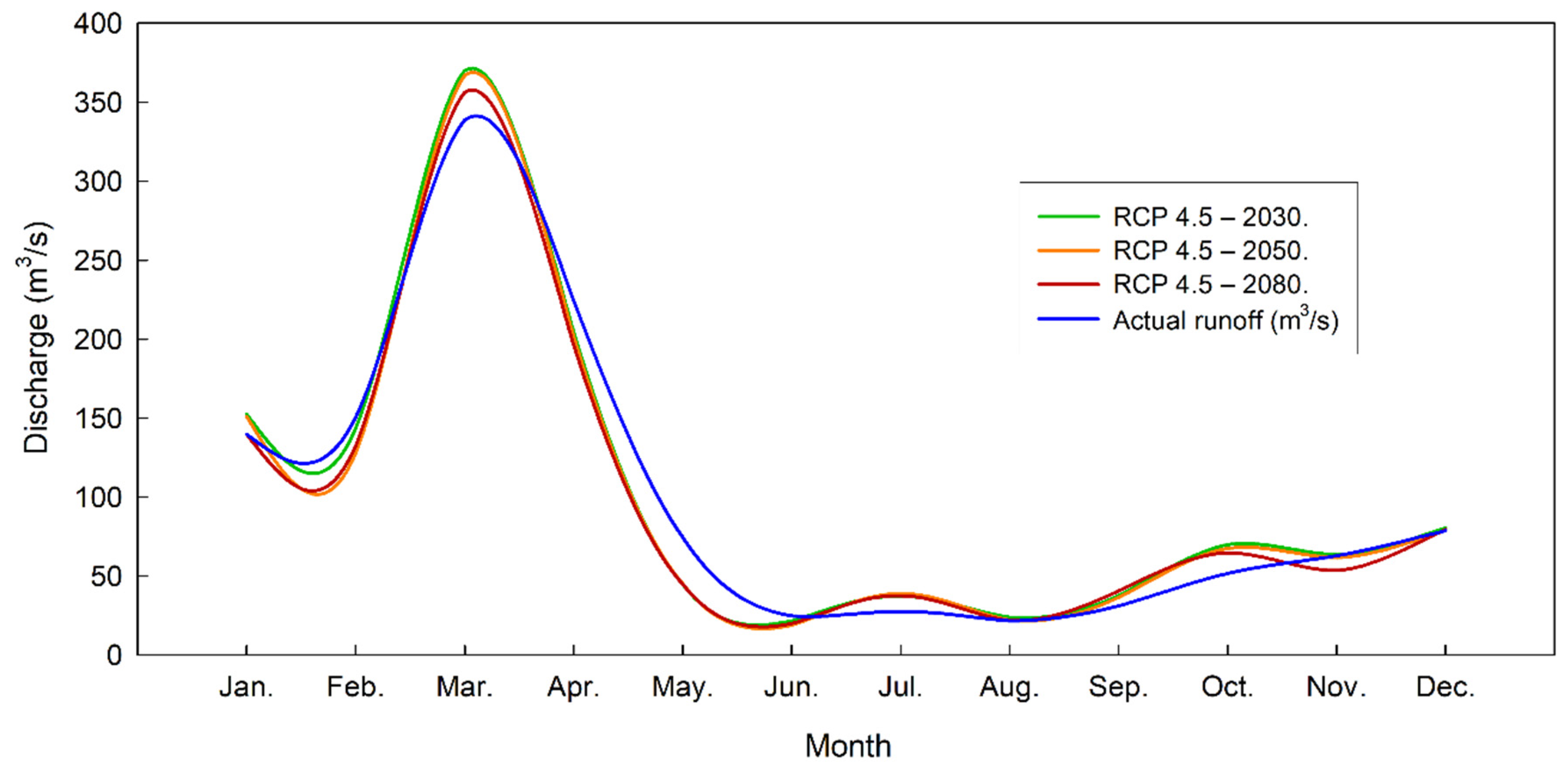
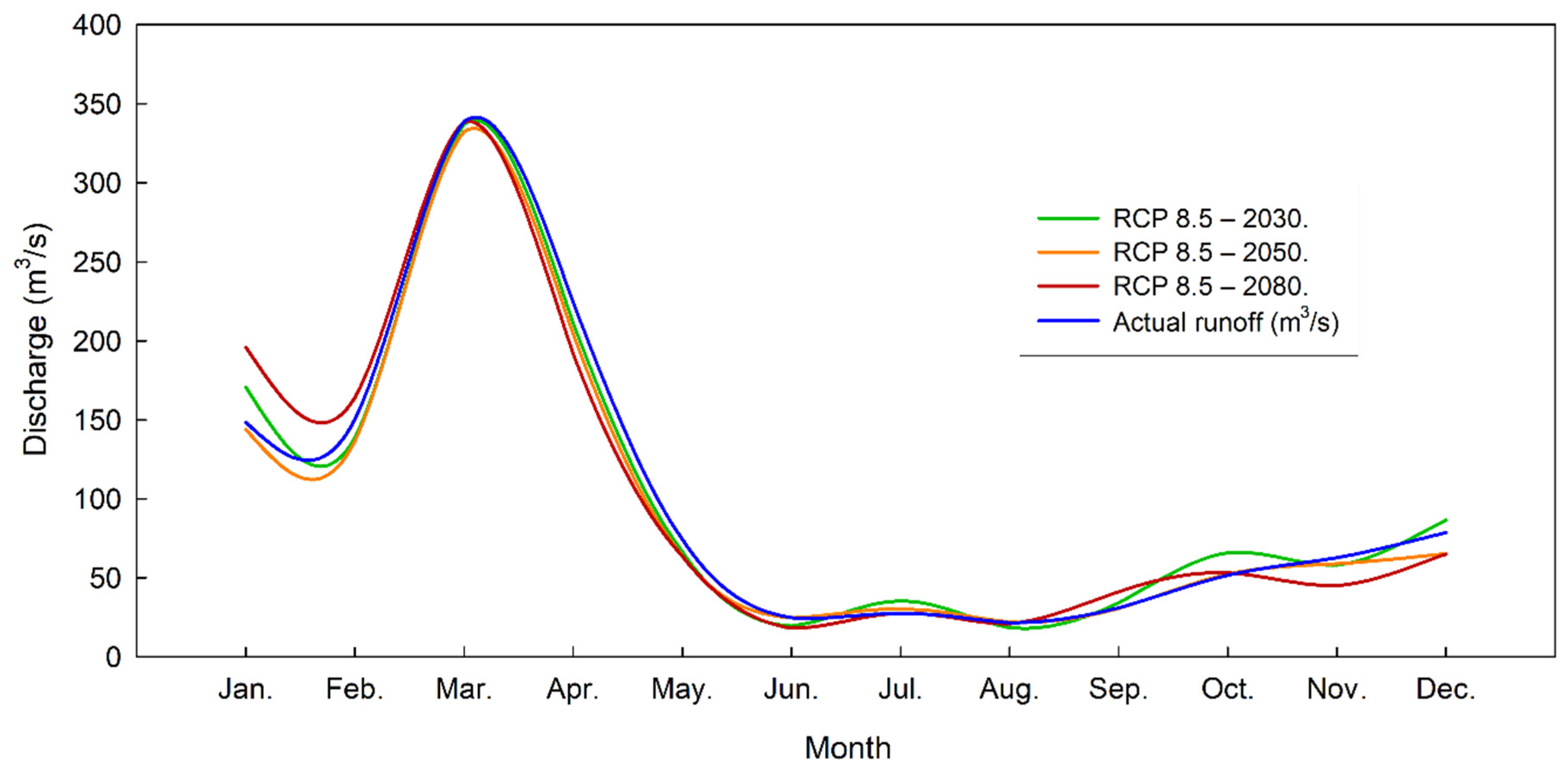
3.4. Climate Change Scenario RCP 4.5 and RCP 8.5

The result of RCP 4.5 showed flow variability between the projected years. In this sense, the highest flow months were from January to May, justified by the wet season, while the lowest flows were reached between June and December (dry season). The average annual discharge reports a decrease over the years of assessment. Namely, for 2030, 2050 and 2080, 104.0, 101.3 and 98.8 m3/s are projected, respectively (Figure 7 and Table S4).
Like the RCP 4.5 scenario, the RCP 8.5 shows that from January to May are the highest flow months, and from June to September as the lowest. In turn, the average flow for 2030, 2050 and 2080 (93.4, 97.1 and 102.1 m3/s), increases with respect to the other years (Figure 8 and Table S5).

4. Discussion

The SRM was used, which has been applied in many river basins analysed under climate change scenarios [1,4,45,49]. The model requires large amounts of data to simulate runoff on a daily scale in catchments where snow and glacier melt dominate the runoff generation process [49]. In this study, it was necessary to use historical data on temperature, precipitation and SCA, which allowed for successful calibration and validation during the baseline period (2005–2009). The SRM projected future changes in runoff in the Santa River sub-basin. The SRM used terrain, snow and climate data to project future changes in runoff from the Santa river sub-basin [50].
For the determination of the SCA, satellite imagery from the MODIS Terra and Aqua sensor was used, which allowed the capture of land surface conditions. These images are potentially important for hydrological studies due to their high spatial and temporal resolution. Nevertheless, they can be affected by high cloud coverage, preventing an accurate estimation of the SCA [51]. Many studies have applied techniques to improve the images and obtain better quality SCA data [52,53]. In the study area, SCA values fluctuated between 5.1 and 7.4% over the total study area, therefore it was necessary to compare with SCA values obtained from Landsat data [54].
Observed data from meteorological stations were used for the simulation of the SRM, whereas data from hydrometric stations were used for the calibration. Flows ranged from 90.0 to 215.0 m3/s, with an acceptable calibration fit for 2005, 2006, 2007, 2008 and 2009. Temperatures below 0 °C during the winter months resulted in little production of meltwater or rainfall to maintain flows during the winter season [13]. The SRM results underestimated the flows in the winter months. This is due to the simplified representation of the recession coefficient as a function of discharge, with the sub-basin more sensitive to high flows due to the presence of precipitation especially between the months of December and March. On the other hand, the SCA increases between April and August with decreasing temperature. Conversely, it decreases between September and November as in the published study by Adnan et al. [45]. On the other hand, surface flow increases in the summer season, which is mainly related to the availability of thermal energy that melts the SCA [55], and it may also reflect global warming caused by anthropogenic activities [29,56].
According to the projections, there will be an increase in precipitation and temperature compared to current conditions. Flow is projected to decrease by 2080 in the PCR 4.5 and PCR 8.5 scenarios (TS4 and TS5). The SCA has been reduced by more than 30% since 1930 with a marked retreat of glaciers over the last decades, as glaciers act as a temporary water store for precipitation that falls as snow during the rainy season and is discharged in the dry season, regulating the lack of water in the lower sub-basin due to the scarcity of precipitation [29].
Climate change has been shown to have a negative effect in high Andean areas by increasing the retreat of glaciers [49]. Air temperature has a significant influence on the energy balance, although not through sensible heat flux, but indirectly through rain-snow fluctuations [35]. Likewise, the projected climate change scenarios of RCP 4.5. and RCP 8.5 for 2030, 2050 and 2080, indicate a retreat of the SCA in the short term, and it is that as glaciers retreat and lose mass, a temporary increase in run-off is added, which raises serious concerns on sustainability, which is corroborated with the results reported by Bury et al. [38] and Baraer et al. [57]. These changes are significantly altering the availability of water in the region and pose critical risks for the population and for human activities (tourism, hydroelectric power, agriculture and livestock, large-scale irrigation) [35,38,58]. If the already scarce water resources of the poor population of the Santa Valley diminish further, conflicts over water could increase in the near future.
This study presents a tool for taking action against the melting of glaciers and conservation of water resources. The application of SRM in tropical ecosystems presented reliable results. Likewise, the integration of remote sensing tools such as GEE has been important to obtain the SCA. The information generated can be used by authorities and decision-makers in the design of strategies and policies focused on prevention, control and conservation. of water resources. Finally, this methodology can be applied to other glacier areas with certain adjustments in the methodology.

5. Conclusions

The SRM was used to simulate the runoff of the Santa River sub-basin during the reference period 2005–2009, using the snow cover product MOD10A1 and climatic data of temperature and precipitation. After successful calibration and validation during the baseline period, the model was applied to project future changes in runoff from the sub-basin. In general, the Santa River runoff decreases during the summer months and increases the rest of the year. The results show a substantial increase in runoff projected for January to May. Furthermore, the largest increases in flow occur between March and April, experiencing the greatest reduction in SCA area and the lowest months from June to August.
The SRM is a tool that allows hydrological modelling of alpine and tropical watersheds, using remote sensing data and GCM can be extended to assess the impact under climate change scenarios. Finally, the prediction of the runoff of a basin facilitates the understanding of the processes of deglaciation and scarcity of the water resource, which allows proposing alternatives for prevention, control and conservation.

Supplementary Materials

The following are available online at https://www.mdpi.com/article/10.3390/w13243535/s1, Table S1: Characteristics of the six elevation zones extracted from the DEM of the Santa River sub-basin; Table S2: Snow cover area in km2 generated with MODIS10A1 sensor imagery every 1 days at GEE; Table S3: Values of the climatic variables of precipitation, temperature, SCA and discharge for the SRM from 2005 to 2009; Table S4: Monthly average discharge under climate change scenario RCP 4.5; Table S5: Monthly average discharge under climate change scenario RCP 8.5.

Author Contributions

Conceptualization, E.C., A.M. and E.T.; Data curation, E.C., A.M., F.C. (Fredy Calizaya), E.B. and E.T.; Formal analysis, E.C. and E.T.; Funding acquisition, E.C., A.M., F.C. (Fredy Calizaya), E.B., F.C. (Fernando Corroto), R.S., H.V. and E.T.; Investigation, E.C., A.M., F.C. (Fredy Calizaya), E.B., F.C. (Fernando Corroto), R.S., H.V. and E.T.; Methodology, E.C., A.M., E.B. and E.T.; Project administration, E.C., A.M. and E.T.; Resources, A.M., F.C. (Fredy Calizaya), F.C. (Fernando Corroto), R.S. and H.V.; Software, E.C. and E.T.; Supervision, E.C., A.M., F.C. (Fredy Calizaya), F.C. (Fernando Corroto), R.S., H.V. and E.T.; Validation, A.M., F.C. (Fredy Calizaya), F.C. (Fernando Corroto), R.S., H.V. and E.T.; Visualization, A.M., F.C. (Fredy Calizaya), F.C. (Fernando Corroto), R.S. and H.V.; Writing—original draft, E.C., E.B. and E.T.; Writing—review & editing, E.C., A.M., F.C. (Fredy Calizaya), E.B., F.C. (Fernando Corroto), R.S., H.V. and E.T. All authors have read and agreed to the published version of the manuscript.

Funding

This research was funded by Universidad Nacional Agraria La Molina (UNALM), Universidad Nacional del Altiplano de Puno (UNAP) and Instituto Nacional de Innovación Agraria (INIA).

Institutional Review Board Statement

Not applicable.

Informed Consent Statement

Not applicable.

Data Availability Statement

Not applicable.

Acknowledgments

The main author thanks his father Benigno Gregorio Calizaya Ticona who passed away on 26 January 2020, because I owe many of my achievements to you. Thank you for having shaped me as the person I am. The authors thank Blair Fitzharris and Pascal Sirguey for providing the temporally interpolated MODIS snow cover product. The authors acknowledge and appreciate the support of the Universidad Nacional Agraria La Molina (UNALM), Research Institute for Sustainable Development in Highland Forests (INDES-CES) of the National University Toribio Rodríguez de Mendoza de Amazonas (UNTRM), Instituto Nacional de Innovación Agraria (INIA), Servicio Nacional de Meteorología e Hidrología del Perú (SENAMHI) and Autoridad Nacional del Agua (ANA). Finally, the authors express their gratitude for the thorough work of the tree anonymous reviewers, who greatly improved the quality of this manuscript.

Conflicts of Interest

The authors declare no conflict of interest.

References

  1. Banerjee, C.; Sharma, A. Decline in terrestrial water recharge with increasing global temperatures. Sci. Total Environ. 2021, 764, 142913. [Google Scholar] [CrossRef] [PubMed]
  2. Blöschl, G.; Hall, J.; Parajka, J.; Perdigão, R.A.P.; Merz, B.; Arheimer, B.; Aronica, G.T.; Bilibashi, A.; Bonacci, O.; Borga, M.; et al. Changing climate shifts timing of European floods. Science 2017, 357, 588–590. [Google Scholar] [CrossRef] [PubMed] [Green Version]
  3. Rosenzweig, C.; Karoly, D.; Vicarelli, M.; Neofotis, P.; Wu, Q.; Casassa, G.; Menzel, A.; Root, T.L.; Estrella, N.; Seguin, B.; et al. Attributing physical and biological impacts to anthropogenic climate change. Nat. Cell Biol. 2008, 453, 353–357. [Google Scholar] [CrossRef] [PubMed]
  4. Kaser, G. A review of the modern fluctuations of tropical glaciers. Glob. Planet. Chang. 1999, 22, 93–103. [Google Scholar] [CrossRef]
  5. Migliavacca, F.; Confortola, G.; Soncini, A.; Senese, A.; Diolaiuti, G.A.; Smiraglia, C.; Barcaza, G.; Bocchiola, D. Hydrology and potential climate changes in the Rio Maipo (Chile). Geogr. Fis. Din. Quat. 2015, 38, 155–168. [Google Scholar]
  6. Zhang, H.; Li, Z.; Zhou, P.; Zhu, X.; Wang, L. Mass-balance observations and reconstruction for Haxilegen Glacier No. 51, eastern Tien Shan, from 1999 to 2015. J. Glaciol. 2018, 64, 689–699. [Google Scholar] [CrossRef] [Green Version]
  7. Hagg, W.; Mayer, C.; Lambrecht, A.; Kriegel, D.; Azizov, E. Glacier changes in the Big Naryn basin, Central Tian Shan. Glob. Planet. Chang. 2013, 110, 40–50. [Google Scholar] [CrossRef]
  8. Pellicciotti, F.; Ragettli, S.; Carenzo, M.; McPhee, J. Changes of glaciers in the Andes of Chile and priorities for future work. Sci. Total Environ. 2014, 493, 1197–1210. [Google Scholar] [CrossRef]
  9. Abudu, S.; Sheng, Z.-P.; Cui, C.-L.; Saydi, M.; Sabzi, H.-Z.; King, J.P. Integration of aspect and slope in snowmelt runoff modeling in a mountain watershed. Water Sci. Eng. 2016, 9, 265–273. [Google Scholar] [CrossRef]
  10. Steele, C.; Dialesandro, J.; James, D.; Elias, E.; Rango, A.; Bleiweiss, M. Evaluating MODIS snow products for modelling snowmelt runoff: Case study of the Rio Grande headwaters. Int. J. Appl. Earth Obs. Geoinf. 2017, 63, 234–243. [Google Scholar] [CrossRef]
  11. Leavesley, G.H. Problems of snowmelt runoff modelling for a variety of physiographic and climatic conditions. Hydrol. Sci. J. 1989, 34, 617–634. [Google Scholar] [CrossRef] [Green Version]
  12. Hock, R. Glacier melt: A review of processes and their modelling. Prog. Phys. Geogr. Earth Environ. 2005, 29, 362–391. [Google Scholar] [CrossRef]
  13. Siemens, K.; Dibike, Y.; Shrestha, R.; Prowse, T. Runoff projection from an alpine watershed in Western Canada: Application of a snowmelt runoff model. Water 2021, 13, 1199. [Google Scholar] [CrossRef]
  14. Hock, R. Temperature index melt modelling in mountain areas. J. Hydrol. 2003, 282, 104–115. [Google Scholar] [CrossRef]
  15. Condom, T.; Escobar, M.; Purkey, D.; Pouget, J.C.; Suarez, W.; Ramos, C.; Apaéstegui, J.; Tacsi, A.; Gomez, J. Simulating the implications of glaciers’ retreat for water management: A case study in the Rio Santa basin, Peru. Water Int. 2012, 37, 442–459. [Google Scholar] [CrossRef]
  16. Shirsat, T.S.; Kulkarni, A.V.; Momblanch, A.; Randhawa, S.; Holman, I.P. Towards climate-adaptive development of small hydropower projects in Himalaya: A multi-model assessment in upper Beas basin. J. Hydrol. Reg. Stud. 2021, 34, 100797. [Google Scholar] [CrossRef]
  17. Han, P.; Long, D.; Han, Z.; Du, M.; Dai, L.; Hao, X. Improved understanding of snowmelt runoff from the headwaters of China’s Yangtze River using remotely sensed snow products and hydrological modeling. Remote Sens. Environ. 2019, 224, 44–59. [Google Scholar] [CrossRef]
  18. Long, D.; Shen, Y.; Sun, A.; Hong, Y.; Longuevergne, L.; Yang, Y.; Li, B.; Chen, L. Drought and flood monitoring for a large karst plateau in Southwest China using extended GRACE data. Remote Sens. Environ. 2014, 155, 145–160. [Google Scholar] [CrossRef]
  19. Kult, J.; Choi, W.; Choi, J. Sensitivity of the snowmelt runoff model to snow covered area and temperature inputs. Appl. Geogr. 2014, 55, 30–38. [Google Scholar] [CrossRef]
  20. Martinec, J.; Rango, A.; Major, E. Snowmelt-Runoff Model (SRM) User’s Manual; NASA: Washington, DC, USA, 2008.
  21. Di Marco, N.; Avesani, D.; Righetti, M.; Zaramella, M.; Majone, B.; Borga, M. Reducing hydrological modelling uncertainty by using MODIS snow cover data and a topography-based distribution function snowmelt model. J. Hydrol. 2021, 599, 126020. [Google Scholar] [CrossRef]
  22. Gascoin, S.; Hagolle, O.; Huc, M.; Jarlan, L.; Dejoux, J.-F.; Szczypta, C.; Marti, R.; Sánchez, R. A snow cover climatology for the Pyrenees from MODIS snow products. Hydrol. Earth Syst. Sci. 2015, 19, 2337–2351. [Google Scholar] [CrossRef] [Green Version]
  23. Engel, M.; Notarnicola, C.; Endrizzi, S.; Bertoldi, G. Snow model sensitivity analysis to understand spatial and temporal snow dynamics in a high-elevation catchment. Hydrol. Process. 2017, 31, 4151–4168. [Google Scholar] [CrossRef]
  24. Parajka, J.; Holko, L.; Kostka, Z.; Blöschl, G. MODIS snow cover mapping accuracy in a small mountain catchment–comparison between open and forest sites. Hydrol. Earth Syst. Sci. 2012, 16, 2365–2377. [Google Scholar] [CrossRef] [Green Version]
  25. Di Marco, N.; Righetti, M.; Avesani, D.; Zaramella, M.; Notarnicola, C.; Borga, M. Comparison of MODIS and model-derived snow-covered areas: Impact of land use and solar illumination conditions. Geosciences 2020, 10, 134. [Google Scholar] [CrossRef] [Green Version]
  26. Klein, A.G.; Barnett, A.C. Validation of daily MODIS snow cover maps of the upper rio grande river basin for the 2000–2001 snow year. Remote Sens. Environ. 2003, 86, 162–176. [Google Scholar] [CrossRef]
  27. Valderrama, P.; Vilca, O. Dinamica e implicancias del aluvión de la laguna 513, Cordillera Blanca, Ancash Perú. Rev. Asoc. Geol. Argent. 2012, 69, 400–406. [Google Scholar]
  28. Zapata, M.; Arnaud, Y.; Gallaire, R. Inventario de glaciares de la cordillera blanca. In Proceedings of the 13th IWRA World Water Congress, Montpellier, France, 1–4 September 2008; pp. 1–4. [Google Scholar]
  29. Schauwecker, S.; Rohrer, M.; Acuña, D.; Cochachin, A.; Dávila, L.; Frey, H.; Giráldez, C.; Gómez, J.; Huggel, C.; Jacques-Coper, M.; et al. Climate trends and glacier retreat in the Cordillera Blanca, Peru, revisited. Glob. Planet. Chang. 2014, 119, 85–97. [Google Scholar] [CrossRef]
  30. Kaser, G.; Juen, I.; Georges, C.; Gómez, J.; Tamayo, W. The impact of glaciers on the runoff and the reconstruction of mass balance history from hydrological data in the tropical Cordillera Bianca, Perú. J. Hydrol. 2003, 282, 130–144. [Google Scholar] [CrossRef]
  31. Hänchen, L.; Klein, C.; Maussion, F.; Gurgiser, W.; Wohlfahrt, G. Vegetation indices as a proxy for spatio-temporal variations in water availability in the semi-arid Rio Santa valley (Callejón de Huaylas, Peru). In Proceedings of the EGU General Assembly 2021 (EGU21-8330), Online, 19–30 April 2021. [Google Scholar] [CrossRef]
  32. Lynch, B.D. Vulnerabilities, competition and rights in a context of climate change toward equitable water governance in Peru’s Rio Santa Valley. Glob. Environ. Chang. 2012, 22, 364–373. [Google Scholar] [CrossRef]
  33. ANA. Inventario de Glaciares Coordillera Blanca; ANA: Lima, Peru, 2010; Available online: https://repositorio.ana.gob.pe/bitstream/handle/20.500.12543/490/ANA0000276.pdf?sequence=1&isAllowed=y (accessed on 1 October 2017).
  34. Vuille, M.; Kaser, G.; Juen, I. Glacier mass balance variability in the Cordillera Blanca, Peru and its relationship with climate and the large-scale circulation. Glob. Planet. Chang. 2008, 62, 14–28. [Google Scholar] [CrossRef] [Green Version]
  35. Vuille, M.; Francou, B.; Wagnon, P.; Juen, I.; Kaser, G.; Mark, B.G.; Bradley, R.S. Earth-science reviews climate change and tropical andean glaciers: Past, present and future. Earth-Sci. Rev. 2008, 89, 79–96. [Google Scholar] [CrossRef] [Green Version]
  36. INEI Perú. Estimaciones y Proyecciones de Población por Departamento, Provincia y Distrito, 2018–2020; INEI Perú: Lima, Peru, 2020. Available online: https://www.inei.gob.pe/media/MenuRecursivo/publicaciones_digitales/Est/Lib1715/libro.pdf (accessed on 1 October 2017).
  37. Chevallier, P.; Pouyaud, B.; Suarez, W.; Condom, T. Climate change threats to environment in the tropical Andes: Glaciers and water resources. Reg. Environ. Chang. 2011, 11, 179–187. [Google Scholar] [CrossRef]
  38. Bury, J.; Mark, B.G.; Carey, M.; Young, K.R.; McKenzie, J.M.; Baraer, M.; French, A.; Polk, M.H. New geographies of water and climate change in Peru: Coupled natural and social transformations in the Santa River watershed. Ann. Assoc. Am. Geogr. 2013, 103, 363–374. [Google Scholar] [CrossRef] [Green Version]
  39. Tadono, T.; Ishida, H.; Oda, F.; Naito, S.; Minakawa, K.; Iwamoto, H. Precise global DEM generation by ALOS PRISM. ISPRS Ann. Photogramm. Remote Sens. Spat. Inf. Sci. 2014, 2, 71–76. [Google Scholar] [CrossRef] [Green Version]
  40. Riggs, G.A.; Hall, D.; Román, M.O. MODIS snow products: Collection 6 user guide. Earth Sci. 2016, 6, 1–80. [Google Scholar]
  41. Hall, D.K.; Riggs, G.A.; Salomonson, V.V.; DiGirolamo, N.E.; Bayr, K.J. MODIS snow-cover products. Remote Sens. Environ. 2002, 83, 181–194. [Google Scholar] [CrossRef] [Green Version]
  42. Gorelick, N.; Hancher, M.; Dixon, M.; Ilyushchenko, S.; Thau, D.; Moore, R. Google earth engine: Planetary-scale geospatial analysis for everyone. Remote Sens. Environ. 2017, 202, 18–27. [Google Scholar] [CrossRef]
  43. Riggs, G.A.; Hall, D.K.; Salomonson, V.V. MODIS Snow Products User Guide to Collection 5. Available online: https://modis-snow-ice.gsfc.nasa.gov/uploads/sug_c5.pdf (accessed on 1 September 2017).
  44. Dozier, J. Spectral signature of alpine snow cover from the Landsat thematic mapper. Remote Sens. Environ. 1989, 28, 9–22. [Google Scholar] [CrossRef]
  45. Adnan, M.; Nabi, G.; Poomee, M.S.; Ashraf, A. Snowmelt runoff prediction under changing climate in the Himalayan cryosphere: A case of Gilgit River Basin. Geosci. Front. 2017, 8, 941–949. [Google Scholar] [CrossRef] [Green Version]
  46. Tahir, A.A.; Chevallier, P.; Arnaud, Y.; Neppel, L.; Ahmad, B. Modeling snowmelt-runoff under climate scenarios in the Hunza River basin, Karakoram Range, Northern Pakistan. J. Hydrol. 2011, 409, 104–117. [Google Scholar] [CrossRef]
  47. Zhang, G.; Xie, H.; Yao, T.; Li, H.; Duan, S. Quantitative water resources assessment of Qinghai Lake basin using snowmelt runoff model (SRM). J. Hydrol. 2014, 519, 976–987. [Google Scholar] [CrossRef]
  48. Hoar, T.; Doug, N. Statistical Downscaling of the Community Climate System Model (CCSM) Monthly Temperature and Precipitation Projections; Institute for Mathematics Applied to Geosciences/National Center for Atmospheric Research: Boulder, CO, USA, 2008.
  49. Escanilla-Minchel, R.; Alcayaga, H.; Soto-Alvarez, M.; Kinnard, C.; Urrutia, R. Evaluation of the impact of climate change on runoff generation in an andean glacier watershed. Water 2020, 12, 3547. [Google Scholar] [CrossRef]
  50. Moriasi, D.N.; Arnold, J.G.; Van Liew, M.W.; Bingner, R.L.; Harmel, R.D.; Veith, T.L. Model evaluation guidelines for systematic quantification of accuracy in watershed simulations. Trans. ASABE 2007, 50, 885–900. [Google Scholar] [CrossRef]
  51. Hussainzada, W.; Lee, H.S.; Vinayak, B.; Khpalwak, G.F. Sensitivity of snowmelt runoff modelling to the level of cloud coverage for snow cover extent from daily MODIS product collection 6. J. Hydrol. Reg. Stud. 2021, 36, 100835. [Google Scholar] [CrossRef]
  52. Saleem, J.; Butt, A.; Shafiq, A.; Ahmad, S.S.; Supervisor, A.S. Cryosphere dynamic study of Hunza Basin using remote sensing, GIS and runoff modeling. J. King Saud Univ.-Sci. 2020, 32, 2462–2467. [Google Scholar] [CrossRef]
  53. Hall, D.K.; Riggs, G.A.; Foster, J.L.; Kumar, S.V. Development and evaluation of a cloud-gap-filled MODIS daily snow-cover product. Remote Sens. Environ. 2010, 114, 496–503. [Google Scholar] [CrossRef] [Green Version]
  54. Khan, A.; Naz, B.; Bowling, L. Separating snow, clean and debris covered ice in the Upper Indus Basin, Hindukush-Karakoram-Himalayas, using landsat images between 1998 and 2002. J. Hydrol. 2015, 521, 46–64. [Google Scholar] [CrossRef] [Green Version]
  55. Archer, D. Contrasting hydrological regimes in the upper Indus Basin. J. Hydrol. 2003, 274, 198–210. [Google Scholar] [CrossRef]
  56. Archer, D.R.; Forsythe, N.; Fowler, H.J.; Shah, S.M. Sustainability of water resources management in the Indus Basin under changing climatic and socio economic conditions. Hydrol. Earth Syst. Sci. 2010, 14, 1669–1680. [Google Scholar] [CrossRef] [Green Version]
  57. Baraer, M.; Mark, B.G.; McKenzie, J.M.; Condom, T.; Bury, J.; Huh, K.-I.; Portocarrero, C.; Gómez, J.; Rathay, S. Glacier recession and water resources in Peru’s Cordillera Blanca. J. Glaciol. 2012, 58, 134–150. [Google Scholar] [CrossRef] [Green Version]
  58. Bury, J.T.; Mark, B.; McKenzie, J.M.; French, A.; Baraer, M.; Huh, K.I.; Luyo, M.A.Z.; López, R.J.G. Glacier recession and human vulnerability in the Yanamarey watershed of the Cordillera Blanca, Peru. Clim. Chang. 2010, 105, 179–206. [Google Scholar] [CrossRef] [Green Version]
Figure 1. Location of the Santa river sub-basin in the Cordillera Blanca (Peru). Source: Adapted from Kaser [4].
Water 13 03535 g001
Figure 2. Flow chart of methodological approach used for the modelling of surface runoff from snowmelt from tropical Andean glaciers under climate scenarios in the Santa River sub-basin (Peru).
Water 13 03535 g002
Figure 3. MODIS image processing and validation of the SCA with Landsat imagery.
Water 13 03535 g003
Figure 4. SCA for MODIS and Landsat comparison data in the Santa River sub-basin. (a) MODIS (17 October 2003); (b) MODIS (6 August 2006); (c) MODIS (17 August 2010); (d) MODIS (21 November 2016); (e) Landsat (17 October 2003); (f) Landsat (6 August 2006); (g) Landsat (17 August 2010); (h) Landsat (21 November 2016).
Water 13 03535 g004
Figure 5. Correlation between standardized values of SCA, precipitation, average temperature and discharge (stations of La Balsa, Quitarcsa and Los Cedros) in the Santa River sub-basin (monthly) (2005–2009). (a) Yanamarey station and (b) Artesonraju AP2 station.
Water 13 03535 g005
Figure 6. Time series and scatter plots for four and a half years the simulation 2005 (a,b), calibration 2006 (c,d), and validation 2007 (e,f), 2008 (g,h) and 2009 (i,j).
Water 13 03535 g006
Figure 7. Simulated discharge in the Santa River sub-basin under changed climate RCP4.5 for 2030, 2050 and 2080.
Water 13 03535 g007
Figure 8. Simulated discharge in the Santa River sub-basin under changed climate RCP 8.5 in the year 2030, 2050 and 2080.
Water 13 03535 g008
Table 1. Total snow cover area in (%) obtained from MODIS and Landsat imagery in the Santa River sub-basin.
Date of ImagesSnow Cover Area (%)
MODIS (500 m)Landsat (30 m)
18 October 20036.16.5
13 May 20046.86.2
6 July 20066.06.1
7 August 20065.85.9
9 June 20086.36.5
15 August 20096.96.4
18 August 20105.45.7
5 August 20116.05.6
12 July 20146.76.2
17 September 20155.75.1
23 January 20164.85.6
22 November 20164.65.2
Table 2. Statistical results of analysis of year-round simulation in SRM, from 2005 to 2009 in the Santa River sub-basin.
Statistical Parameter20052006200720082009
Measure Runoff Volume (106 m3)253,704.003310.983306.033082.623082.62
Average Measured Runoff (m3/s)80.45104.99104.8397.4897.48
Computed Runoff Volume (106 m3)2436.693308.713284.963076.933076.93
Average Computed Runoff (m3/s)77.27104.92104.1797.3097.30
Coefficient of Determination R2 Nash-Sutcliffe0.800.890.840.910.87
Coefficient of Determ. R2 Log (Nash-Sutcliffe)0.670.830.760.920.94
Volume Difference (%)3.950.070.640.180.18
Publisher’s Note: MDPI stays neutral with regard to jurisdictional claims in published maps and institutional affiliations.

