
Teaching-Learning-Based Optimization of Neural Networks for Water Supply Pipe Condition Prediction


1
Construction and Project Management Research Institute, Housing and Building National Research Centre, Giza 12311, Egypt
2
Structural Engineering Department, Faculty of Engineering, Cairo University, Giza 12613, Egypt
3
Department of Buildings, Civil and Environmental Engineering, Concordia University, Montreal, QC H3G 1M8, Canada
4
Department of Architecture & Environmental Planning, College of Engineering & Petroleum, Hadhramout University, Mukalla 50512, Yemen
5
Department of Architecture and Building Science, College of Architecture and Planning, King Saud University, Riyadh 11421, Saudi Arabia
*
Author to whom correspondence should be addressed.
Water 2021, 13(24), 3546; https://doi.org/10.3390/w13243546
Submission received: 14 September 2021
/
Revised: 28 November 2021
/
Accepted: 8 December 2021
/
Published: 11 December 2021
(This article belongs to the Section Urban Water Management)
Abstract
:The bulk of water pipes experience major degradation and deterioration problems. This research aims at estimating the condition of water pipes in Shattora and Shaker Al-Bahery’s water distribution networks, in Egypt. The developed models involve training the Elman neural network (ENN) and feed-forward neural network (FFNN) coupled with particle swarm optimization (PSO), genetic algorithms (GA), the sine cosine algorithm (SCA), and the teaching-learning-based optimization (TLBO) algorithm. For the Shattora network, the inputs to these models are pipe characteristics such as length, wall thickness, diameter, material, lining and coating, surface type, traffic distribution, cathodic protection, flow velocity, and c-factor. For the Shaker Al-Bahery network, the data gathered include length, material, age, diameter, depth, and wall thickness. Three assessment criteria are used to evaluate the suggested machine learning models, namely index of agreement (IOA), correlation coefficient (R), and root mean squared error (RMSE). The results reveal that coupling FFNN with the TLBO algorithm outperforms other prediction models. Therefore, the FFNN-TLBO model can be a valuable tool for simulating the water network pipe condition. This study could help the water municipality allocate the available budget effectively and plan the required maintenance and rehabilitation actions.
1. Introduction
The water supply system is the cornerstone of the nation’s resources. Environmental, physical, and operational factors compromise the integrity, reliability, and serviceability of water pipes around the world [1,2]. The fundamental physical factors that govern water pipe failures (e.g., breaks, bursts, leaks, and circumferential and longitudinal cracks) include its material, length, diameter, thickness, and vintage [3,4]. However, these failures are exacerbated by external factors such as climate conditions, traffic loads, and soil type and temperature [5,6,7]. Finally, operational conditions related to water quality and hydraulic pressure play an essential role in developing water pipeline failures [1,6]. Water network malfunction skews access to clean drinking water in urban areas. Furthermore, it often results in infrastructure disruption, traffic and business disturbances, and other disasters in the surrounding area [8,9].
Most water pipes are approaching or have already reached the end of their useful lives [10]. The ASCE 2021 Report Card rated the condition of infrastructure assets a grade of “C-” for almost two decades. However, the average American household would spend $3300 a year by 2039 to pay for America’s overdue infrastructure bill. Furthermore, the drinking water systems were assigned a “C-” grade. The report estimated the occurrence of water main breaks every two minutes, resulting in the loss of 6 billion gallons of water in the United States. The cumulative investment needs for this asset were predicted to be $1045, but only $611 were available, resulting in a funding gap of $434 during the period of 2020–2029 [11]. Meanwhile, 41% of North America’s water infrastructure was subjected to an increasing breakage rate of 40% over the same period [12]. According to the 2019 Canadian Infrastructure Report Card, 30% of water infrastructure was in extremely good condition, 40% was in good condition, and 25% was in average, bad, or very poor condition [13]. The current funding in the management of water infrastructure was reported to be inadequate to satisfy increasing demands [12].
The degradation of water assets in developing countries is also costing them millions of dollars. Leakages and water losses account for roughly 25% of the water supply in Qatar [14]. Meanwhile, non-revenue water accounts for 35 to 50% of the total water production in Malaysia [15]. This problem imposes a financial burden on the water municipalities. Egypt has a water scarcity of about 7 billion cubic meters per year [16]. According to the Central Agency for Public Mobilization and Statistics (CAPMAS), the percentage of water losses was 29.7% in 2017–2018 [17]. As stated by the National Water Resources Plan of Egypt 2037 and the Ministry of Water Resources and Irrigation, drinking water usage is estimated to be approximately 10 billion m3 per year. Each year, about 3.5 billion m3 of treated water is lost due to leakage from distribution networks, theft, and poor metering, with a projection of 35% of water losses in the system. Based on the Holding Company for Water and Waste Water (HCWW), the overall yearly loss to water utilities is estimated to be 4.5 billion Egyptian pounds. Without any further expenditure, saving half of this money would provide water to an additional 11 million people [18]. The Egyptian government has set aside $57.55 billion for water management projects over the next 20 years [19]. This highlights that water infrastructure assets are being heavily invested in both developed and developing countries. Therefore, it is necessary to establish a new approach for monitoring and maintaining these networks for the benefit of the population and society [20]. This could lead to enhanced asset performance, improved customer service, lower asset outage times, decreased operation and maintenance costs, and greater profitability for the municipality [21,22].
In response to network failures, water service providers either use reactive or proactive maintenance and rehabilitation techniques [23]. Reactive solutions focus on testing the water pipes daily or reporting failures by consumers. Proactive approaches, on the other hand, assess the likelihood of water pipe failure. This allows water municipalities to plan for possible circumstances, such as traffic disruption and breakdown effects [24]. Municipalities have been undertaking monitoring plans and strategic actions to reduce the water network breaks. However, it is impossible to prevent all pipe failures. This emphasizes the importance of developing predictive models by government bodies in order to optimize water system repair and restoration operations [22,25].
The major objective of this research is to estimate the structural condition of pipes in Shattora and Shaker Al-Bahery water distribution networks, Egypt, using Elman neural networks (ENN) and optimized feed-forward neural network (FFNN) models. The optimization algorithms involve the particle swarm optimization (PSO) algorithm, genetic algorithms (GA), sine cosine algorithm (SCA), and teaching-learning-based optimization (TLBO) algorithm. The forecasting capabilities of the models are examined using three assessment criteria, namely: the index of agreement (IOA), correlation coefficient (R), and root mean squared error (RMSE). The proposed model acts as an assistance tool for water municipalities to track and monitor the condition of water pipes, plan the required intervention strategies, and manage the allocated budget efficiently.
2. Literature Review
Water breakage, condition, remaining useful life, and risk assessment models have been reviewed in the literature [26]. In the last two decades, transient test-based techniques (TTBTs) have been proposed for fault detection in pressurized pipe systems. Such techniques are based on the properties of pressure waves propagating in a pressurized flow. Accordingly, the measured pressure response can be used to determine the location and size of the fault (e.g., leak, partial blockage, and wall deterioration). Precisely, this approach is based on the behavior of the negative pressure wave created by a fault and its location can be determined from the wave arrival times observed at two or more measurement sections. TTBTs have been used successfully not only in the lab but also in real pipe systems [27,28,29,30,31].
Focused on the water supply suspension risk, Kim et al. [32] proposed a framework for estimating the benefits of water pipe renewal. Some value assessment approaches were less direct and descriptive than the suggested approach based on five benefit items. In addition, a technique for calculating the optimum renewal point was proposed based on the pipe failure rate. This research could be used to establish potential water pipe replacement plans. Kim et al. [33] researched how to boost the water delivery system efficiency. The pipes were first divided into three groups: no strengthening, increased pipe longevity, and installing valves on both ends. Then, two rules were applied, which improved the pipe with the lowest reliability and decreased the number of consumers that were out of service. Considering the small budget and site conditions, the proposed framework paved the way for improving network performance.
Failure prediction and risk management models for water pipes have attracted significant attention from researchers. Machine learning predicts new samples by building a model from input variables and learning the trend between inputs and outputs. It has also gained popularity for simulating dynamic nonlinear interactions between input attributes and outcomes [34]. Diverse research studies predict the residual life for pipelines, which could be defined as the estimated time before a pipe experiences a failure mode that makes its use impossible or impractical [35]. Cortez [36] chose the linear regression model developed by Clark et al. [37] to evaluate the time from installation to the first failure. The reason was that the required data for this model are usually available through the municipality. The model included data on the pipe age, expected service life, diameter, material, length, internal pressure, percent covered by residential areas, percent covered by industrial areas, and breakage history. The model attempted to incorporate additional factors to alleviate uncertainty in a pipe’s service life. However, the inclusion of more exhaustive data such as soil pH might render the assessment infeasible. Zangenehmadar and Moselhi [38] developed an artificial neural network (ANN) model based on the Levenberg–Marquardt backpropagation method to estimate the residual lives of water pipes. The model incorporated data on the pipe length, diameter, material, condition, breakage rate, and age. The results revealed that the most relevant parameters in predicting remaining useful life were pipeline length, age, material, condition, diameter, and breakage rate.
Using multiple machine learning algorithms, Elshaboury and Marzouk [39] predicted the structural condition of water pipes using feed-forward and general regression neural networks (GRNN), multiple linear regression, and support vector regression. The specified input parameters for model development were pipe length, diameter, and wall thickness. Cross-validation was used to assess the performance of the aforementioned models by evaluating the coefficient of determination and root mean squared error. The GRNN outperformed the other models in terms of the evaluation metrics. To forecast the pipe failure probability, Zhang and Ye [40] compared the regression analysis, machine learning, genetic algorithms, and data mining approaches. A tree-based optimization approach was proposed as a data mining technique. Environmental and physical characteristics as well as failure records were taken into account in these methods. A high fitting degree was achieved, indicating the ability of the proposed model to forecast failure risks.
Fan et al. [41] built machine learning models to detect water network leakages. The findings showed that a neural network could reliably distinguish leaking and non-leaking conditions. The results affirmed the high accuracy of the autoencoder (AE) neural network model in detecting leaks occurring in monitored pipes. However, it was difficult for a real water network to operate under normal service conditions. This observation would serve as a reference for placing tracking sensors in the desired area. Jara-Arriagada and Stoianov [42] determined the impact of pressure control on minimizing pipe breaks using logistic regression and a sensitivity analysis. This approach was developed and validated using a broad dataset of historic pipe breaks. By lowering the mean load, pipe failures could be decreased by 18 to 30%. Reduced pressure ranges might have a greater effect on all pipe materials. These results indicated that measuring hydraulic pressure proactively may significantly impact network performance.
Poisson regression and spatiotemporal clustering methods were used by Martínez García et al. [43] to examine the influence of pipe material, diameter, and internal pressure on pipe integrity. The maximum pressure parameter was statistically significant in some districts, while the material parameter was statistically significant in all districts. Ravichandran et al. [44] used machine learning approaches to detect leaks for water mains. In a supervised learning technique, several detection functions originating from acoustic signals were used. The preferred method involved a multi-strategy ensemble learning (MEL) using a gradient boosting tree (GBT) classification model. This method improved the efficiency in optimizing the detection rate compared to k-nearest neighbor and neural networks. Several GBT classifiers were integrated to achieve further enhancements. The suggested MEL solution showed a dramatic increase in efficiency, resulting in a one-order-of-magnitude decrease in false-positive results.
Optimization algorithms have emerged to address water infrastructure asset problems. Awe et al. [45] developed an optimization algorithm to determine the least cost system parameters while satisfying the hydraulic and heuristic rules and constraints. The model was simulated using different pipe diameters and pressure head characteristics. The results yielded the optimum reservoir height and pipe diameter that reduced the total cost of installation, operation, and maintenance of the network. Elshaboury et al. [46] optimized the maintenance and rehabilitation strategies for water pipelines using the GA and PSO algorithm. The optimization model aimed at minimizing the costs of intervention actions and maximizing the network structural condition. The results indicated that the PSO algorithm yielded better results compared to GA. In another study, Elshaboury et al. [47] prioritized the required intervention strategies for water pipelines using a set of meta-heuristic algorithms. These algorithms include the PSO, modified invasive weed optimization, shuffled frog leaping, and artificial bee colony algorithms. The results revealed that the proposed modified algorithm exhibited better results when compared to the aforementioned algorithms.
Some of the previous deterioration models overlooked some important attributes like environmental and operational factors. However, these attributes exert considerable influence on the performance condition of water pipes. Furthermore, conventional machine leaning models such as backpropagation ANN and ENN are highly vulnerable to local minima entrapment and poor convergence which hinder their search abilities. In an attempt to address these shortcomings, the major contributions of this research are identified as follows:
- Incorporating physical, environmental, and operational factors to estimate the condition of water pipelines.
- Estimating the network condition using conventional and hybrid prediction models (i.e., machine learning models coupled with optimization algorithms).
- Reducing the error reported by the optimized FFNN, ENN, and GRNN in the literature by more than 1%, 19%, and 80%, respectively.
3. Materials and Methods
3.1. Elman Recurrent Neural Network
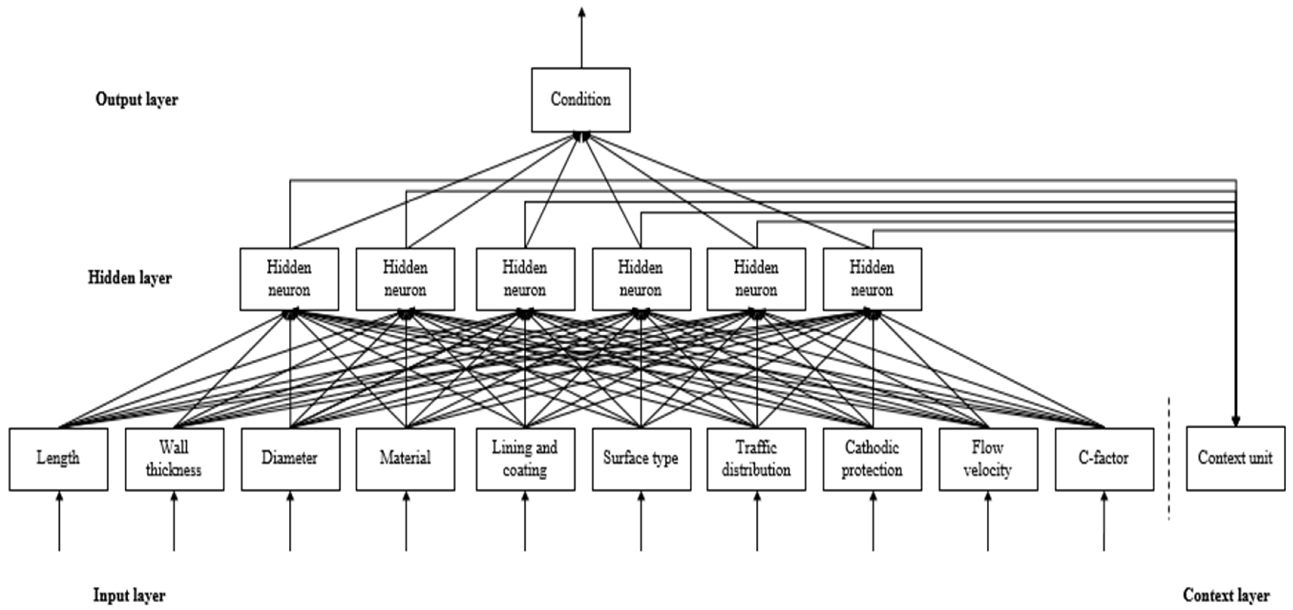
The Elman neural network (ENN) is characterized by changeable feed-forward connections and fixed recurrent connections. The connections are mostly feed-forward, but there are a few feedback connections that allow the network to retain recent cues. The inclusion of a feedback loop has a significant impact on the network’s learning capability. The network also has several user-controlled features, such as training functions and the number of nodes in each layer. As shown in Figure 1, an input layer, an output layer, a hidden layer, and a context layer make up the network architecture. The input layer is split into two parts: true input units and context units, which store a duplicate of the hidden units’ activations from the previous time step. Backpropagation can be used to train the feed-forward connections because the feedback connections are fixed. The network can recognize sequences and can construct short continuations of previously recognized sequences [48].
3.2. Feed-Forward Neural Network
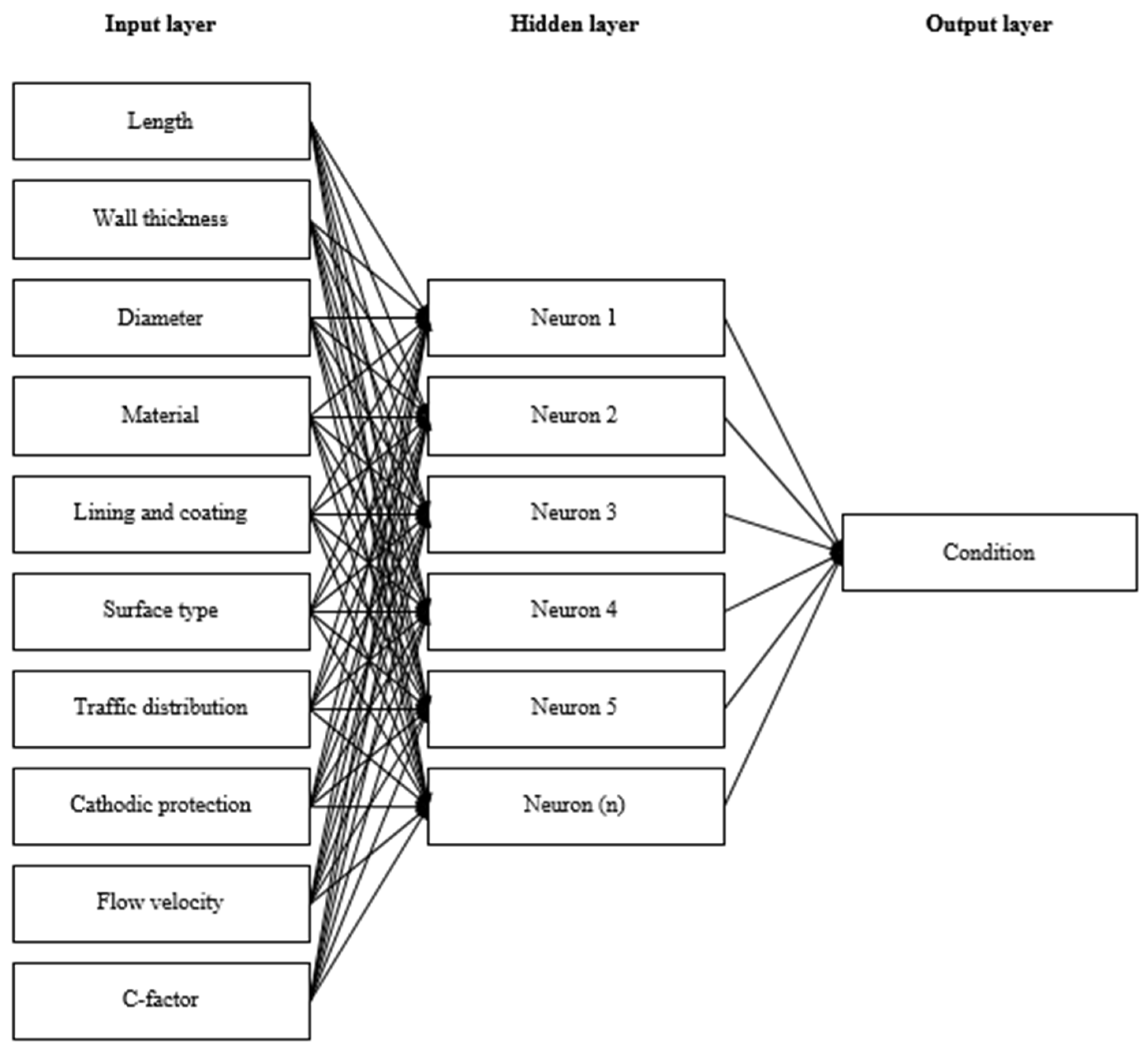
ANN is an area of machine learning in which the algorithms are based on the anatomy of the human brain. The FFNN architecture is shown in Figure 2. This network is fed with input data that are processed using hidden layers to produce the desired output. It is composed of layers of neurons [49]. The input layer receives the input while the output layer predicts the outcome [50]. The hidden layers execute most of the required computations by the network. Channels connecting neurons of successive layers are assigned initial weights. The inputs are multiplied by the weights assigned to them, and the sums are transmitted to the hidden layer neurons. Aside from that, each of these neurons has a bias value that is applied to the input total. This value is then passed through an activation/transformation function which determines the activation status of the neuron. Over the channels, an active neuron communicates data to the neurons of the following layer. The data are forward propagated in this fashion until the result is presented in the last layer. By comparing the projected output to the actual outcome, the network is trained. The weights are then modified based on the backpropagation of the prediction error. The processes of forward and backward propagation are iteratively performed until the network can properly anticipate the output [51]. In summary, the benefits of ANN include the ability to train and adjust the network using historical data. On the other hand, where the structure and network architecture are not specific, the network training speed is slow [52,53].
3.3. Optimization Algorithms
In this research, the FFNN is trained using four optimization algorithms: GA, PSO, SCA, and TLBO. A brief description of each algorithm is provided in the next sub-sections.
3.3.1. Genetic Algorithm
GA has proved its capability to explore and navigate search spaces looking for optimal combinations of solutions. In another way, it is a vast optimization tactic that looks for a robust solution against fitness criteria. It is a search and optimization technique based on Darwin’s principle of natural selection [54]. The procedure begins with a population of randomly formed chromosomes. Selection is the population improvement or survival of the fittest operator; it duplicates individuals with the highest fitness functions and deletes parents with the least fitness functions. In this biological model, a chromosome is filled with genes. In each generation, parents mate and create new chromosomes for their children through cross-over events that mix and match the genes from the parents’ chromosomes. This leads to the survival of the best individuals and their selection to pass on their genes. Otherwise, individuals that are poorly suited to the environment are thrown out over a large number of generations. In this way, nature optimizes a population to best suit the environment it lives in. In order to preserve generational diversity, mutation creates new individuals that are similar to current ones with a small pre-specified probability. Finally, the chromosomes of the last population are chosen as the best solution [47].
3.3.2. Particle Swarm Optimization
PSO is considered one of the well-known evolutionary algorithms. In addition, it has been widely used in a variety of applications in science and industry fields. This algorithm mimics the navigation and movement of a school of fish or flock of birds [55]. It finds a global optimum by creating a population of particles/solutions in the search space. Each particle is composed of three vectors that record the particle’s current location, the best location in the whole swarm, and the traveling direction for each particle. The movement of a particle is affected by its optimal local location and the experience of its neighbors. When neighboring particles find better locations in the search space, the global best position in the solution space is modified. This serves as a reference to help the swarm find the best solution [56]. Finally, the current best location of the particles in the last movement iteration is regarded as the optimum solution.
3.3.3. Sine Cosine Algorithm
SCA is inspired by the mathematical features of sine and cosine trigonometric functions. It includes the primary two approaches (i.e., local and population search strategies) for creating an intelligent algorithm that can successfully search using the local exploitation and global exploration search strategies. The major six steps of this algorithm are listed as follow: (1) initialize a set of candidate solutions, (2) evaluate the fitness of each candidate solution, (3) initialize the algorithm parameters, (4) update each solution using the search equation, (5) update the control parameter, and (6) memorize the destination point [57]. This algorithm is characterized by strong features, including powerful neighborhood search characteristics, outperformance when combined with other algorithms, a high convergence velocity, and a robust global search technique. Therefore, SCA is widely applied in various optimization problems because it is simple, flexible, and straightforward to implement. However, it has certain shortcomings, such as a lack of theoretical convergence, premature (early) convergence, and generational probability configuration changes [58].
3.3.4. Teaching-Learning-Based Optimization
TLBO, proposed by Rao et al. [59], is motivated by the behavior of teachers and students in the classroom. The teacher is determined to be the knowledgeable and most experienced one who receives the highest score in the class, according to the teaching-learning concept. The teacher is in charge of instructing the students and raising the class average score (known as the teacher phase). However, students receive grades on their acquired information based on the quality of the teacher and students in the class. Meanwhile, each student/learner communicates and mutually interacts with another learner randomly to gain knowledge (known as the student phase). The population in this algorithm is made up of many students. Furthermore, the various topics/subjects are similar to the optimization variables. The learner results are used to assess the fitness function of the optimization problem. Finally, the teacher is chosen as the best answer in the whole population [60]. Except for the population size and the maximum number of iterations, the TLBO algorithm does not require any additional parameters for its functioning. Furthermore, when compared to the abovementioned algorithms, such as GA and PSO, the algorithm is simple to construct and uses less processing memory [61].
3.4. Performance Metrics
The performance of machine learning models can be measured using a variety of metrics. In this research, IOA, R, and RMSE metrics are applied to evaluate the models, as illustrated in the following sub-sections.
3.4.1. Index of Agreement
IOA is a standardized measure of the model’s prediction error and it is determined by multiplying the mean square error to the potential error ratio by the number of data points and subtracting one as per Equation (1). Due to the squared differences in the formula, this index is very sensitive to extreme values. It is worth mentioning that a higher IOA value reflects that the predicted and observed values are in good alignment, and vice versa [62].
where and represent the observed and predicted values, respectively. In addition, and represent the mean observed and predicted values, respectively.
3.4.2. Correlation Coefficient
R is a measure of how closely two models are related as per Equation (2). This metric expresses the direction and strength of a relationship between variables with a value ranging from −1 to +1, with −1 and +1 indicating negative and positive correlations, respectively. Meanwhile, a value of 0 indicates no relationship between the variables [63].
3.4.3. Root Mean Squared Error
RMSE is a measure of the residuals’ standard deviation, where residuals (prediction errors) measure the distance/closeness between observed and predicted data points as per Equation (3). In other words, it indicates how densely the data are clustered around the best fit line. The lower the RMSE value, the better the model’s prediction accuracy and vice versa [64].
4. Model Development
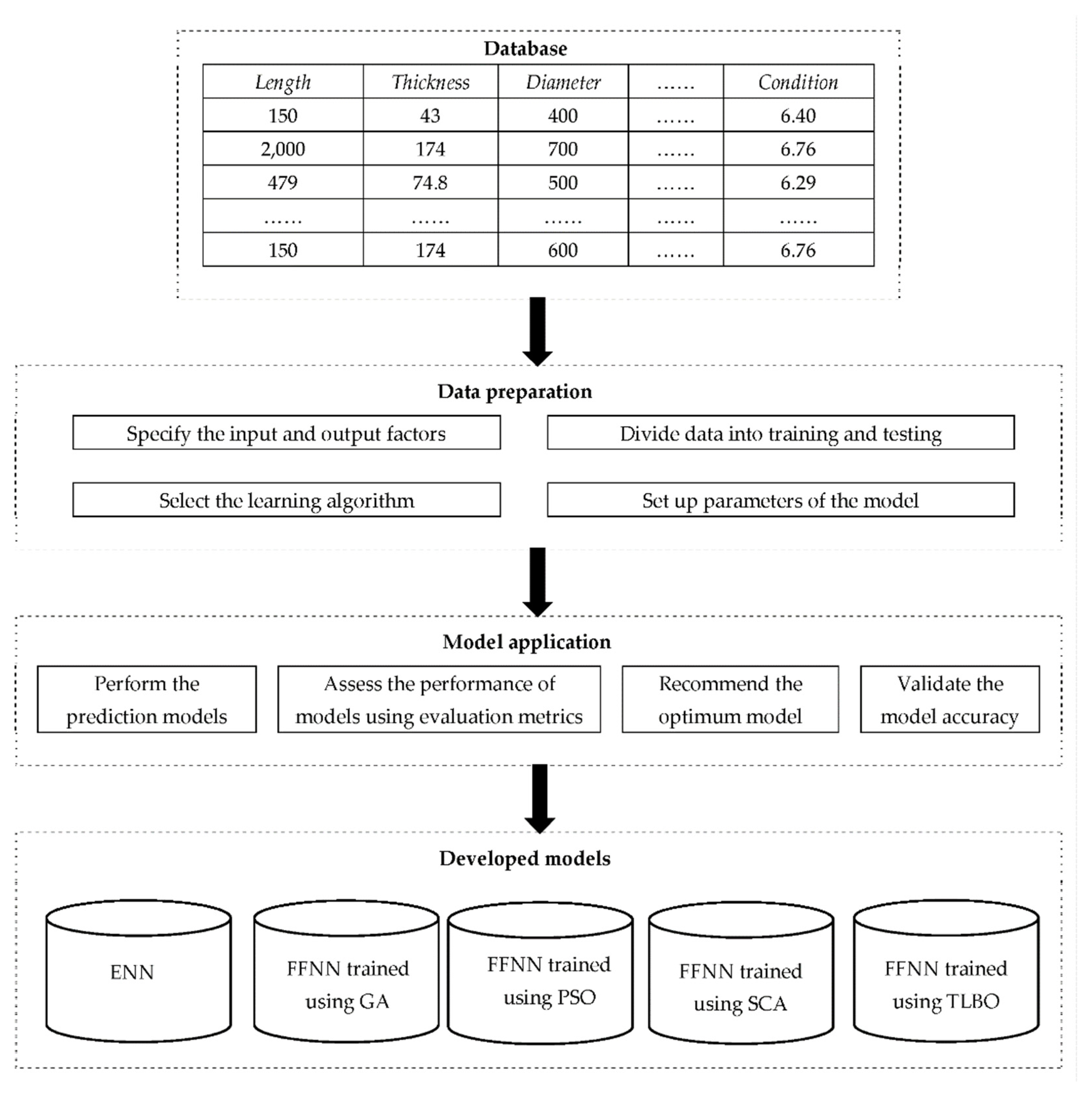
The flowchart for applying machine learning models for predicting water pipe network condition is illustrated in Figure 3. The flowchart starts with preparing the database that comprises the input and output parameters. The data are then divided into training and testing sets to evaluate the models. After selecting the machine learning algorithm and initializing the model parameters, the neural network models are developed and evaluated using performance evaluation metrics to conclude the optimum prediction model.
Pipe characteristics (i.e., input factors) are used to estimate pipe condition (i.e., output factor) using different machine learning models. Equation (4) is used to compute the condition indices of water pipes by multiplying the weight of each factor by the score associated with this factor [65]. The weight reflects the importance of the factor from the expert’s perspective. Questionnaire surveys are undertaken to determine the weight of importance of the condition assessment factors. The experts express their preferences linguistically according to the Saaty fuzzifying scale [66]. The pairwise comparisons are conducted on three levels: (a) between the main categories with respect to the overall condition, (b) between the factors with respect to the main categories, and (c) between the main categories with respect to each other. A fuzzy analytic network process technique is applied to accommodate the interdependencies and uncertainties between the factors. Meanwhile, the contribution of a factor-specific characteristic to the pipe condition index is measured by the factor effect value. The effect values of the influential factors are collected from the literature review [1,65,67]. The computational procedures of determining the condition index are comprehensively described in [68]. This index ranges from 0 to 10, with 0 denoting the most critical condition and 10 denoting the best.
where is the pipe’s condition index, is the factor’s weight of importance, and is the factor’s score that affects the structural condition of the pipes.
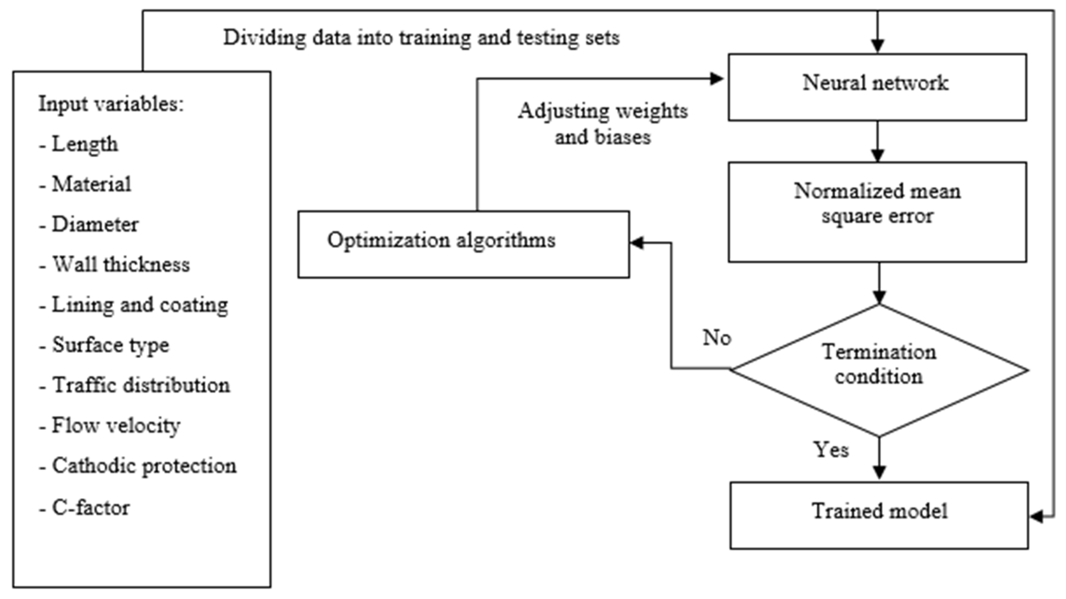
The initial biases and weights’ values in a traditional ANN have a significant effect on the network performance [69]. It is worth mentioning that the neural network may be trained using three approaches [70]: (1) using the fixed network design to manipulate weights and biases, (2) using heuristic algorithms to figure out the best network structure, or (3) using an evolutionary algorithm to modify the parameters of the machine learning model. The PSO, GA, SCA, and TLBO algorithms are used in this research to optimize the randomly specified weights and biases in the FFNN model. When neural networks are combined with optimization algorithms, they improve their ability to solve real-world problems while avoiding overfitting and local minima during training [71]. Figure 4 shows the flowchart of the trained neural network model procedure. To begin training the network, the optimization algorithms initialize the weights and determine their fitness functions. The network fitness is interpreted in this study by calculating the mean square error as per Equation (5). The normalized mean square error is calculated by normalizing the mean square error by the mean target variance as per Equation (6). When the global best solution (i.e., minimal error function) is found, the optimization process ends [72].
where refers to the mean square error, refers to the normalized mean square error, refers to the number of observations, and and refer to the actual and forecasted values, respectively.
The parameters of various algorithms are summarized as follows: the number of iterations and the population size are determined as 1000 and 50, respectively, for all the algorithms. For PSO, the inertia weight, inertia weight damping ratio, personal learning coefficient, and global learning coefficient are equal to 1, 0.99, 2, and 2, respectively. Meanwhile, for GA, the fitness limit and tolerance function are equivalent to 1 × 10⁻⁵ and 1 × 10⁻¹⁰, respectively. Around 70% and 30% of the data are used for training and testing, respectively. The number of hidden neurons is presumed to be 10 for optimized FFNN models. Furthermore, because of its superior performance in solving nonlinear problems, the Levenberg–Marquardt algorithm is chosen as the network training algorithm [52]. The author builds the machine learning models using MATLAB R2019a software.
5. Case Study
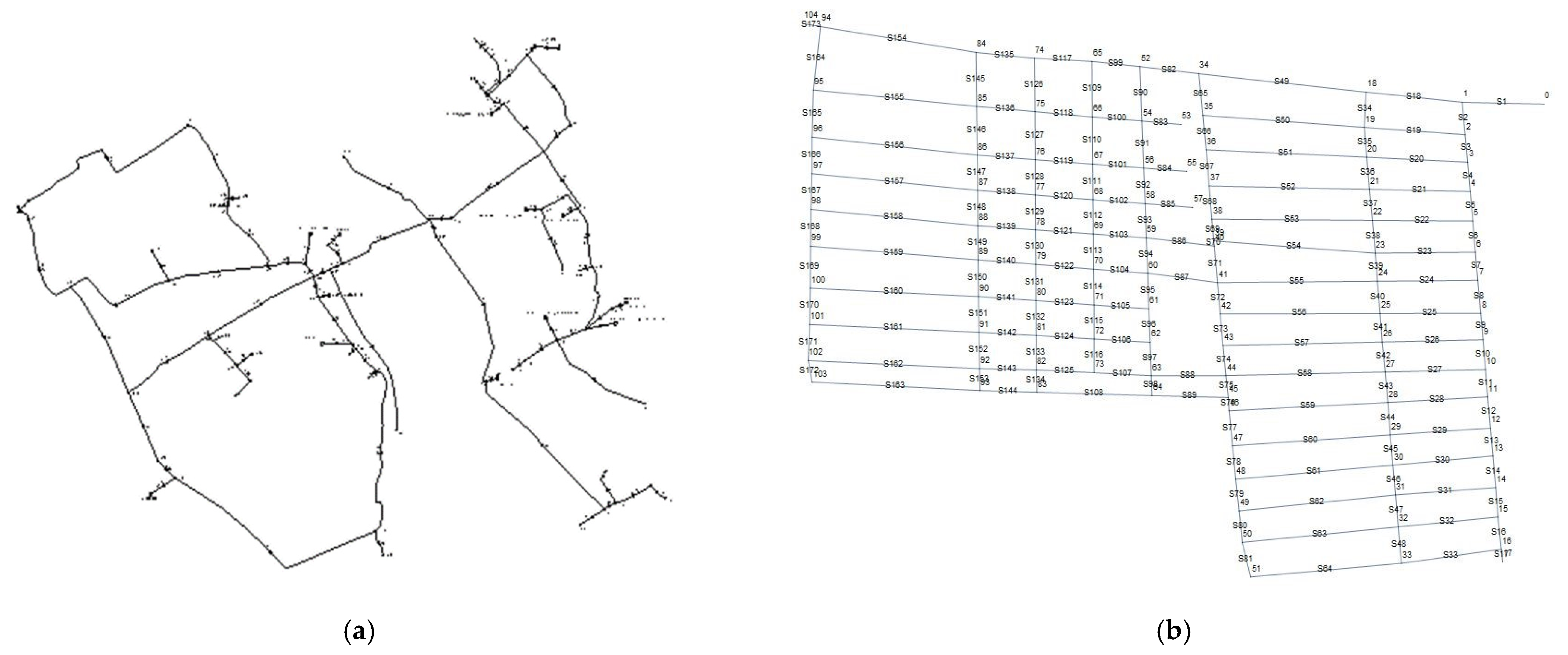
The proposed models are implemented using two water distribution networks in Shattora (Sohag Governorate) and Shaker Al-Bahery (Qalyubia Governorate), Egypt (see Figure 5). The data of the case studies are obtained from the “senior consulting engineers” office [73]. For the Shattora network, the gathered data include physical factors (i.e., length, wall thickness, material, diameter, and lining and coating), environmental factors (i.e., surface type and traffic distribution), and operational factors (i.e., cathodic protection, flow velocity, and c-factor). The network consists of 81 pipelines totaling 106,862 m in length. It shall be noted that the material comprises three different types: uPVC (1), concrete (2), and high-density polyethylene (HDPE) (3). The pipe diameters vary from 200 to 1200 mm, and the wall thickness is determined by the manufacturer’s technical aspects. Moreover, the lining and coating might be lined (1) or unlined (0). For the surface type, it involves asphalt (1) or unpaved (0). In addition, there might be light (1), normal (2), or heavy (3) traffic in this area. Meanwhile, the cathodic protection has only yes (0) or no (1) options. Finally, the c-factor is associated with the pipe material and obtained from the Egyptian code of practice [74]. The input and output factors for the first five pipelines can be found in Table 1. Table 2 depicts statistical parameters for the quantitative input and output variables.
For the Shaker Al-Bahery water network, the data gathered include physical characteristics of the pipes such as length, material, age, diameter, depth, and wall thickness. The network consists of 173 pipes totaling 10.3 km in length. The network pipes are all composed of uPVC and are 1.3 m in depth. They were installed in this neighborhood at the age of 12 years old. Their diameters range from 100 to 400 mm, and the wall thickness is determined by the manufacturer’s technical criteria. Table 3 lists the input and output factors for five pipelines. The statistical parameters for the input and output variables are shown in Table 4.
6. Results and Discussion
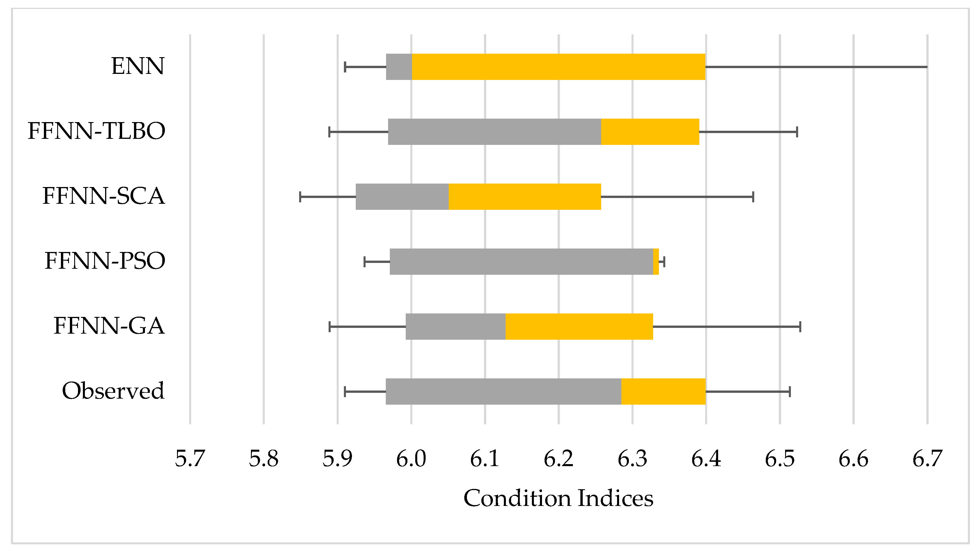
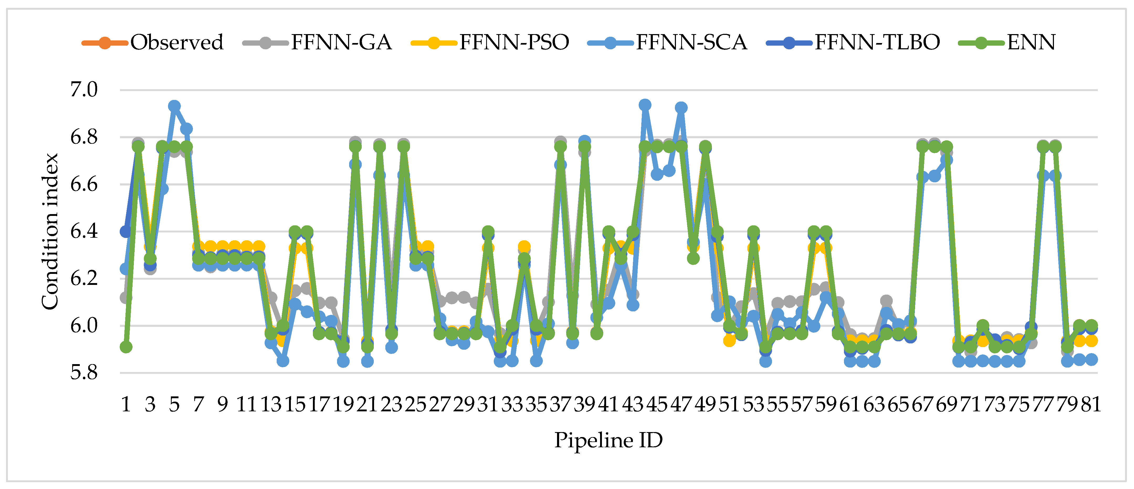
The performance of the ENN and FFNN models coupled with four optimization algorithms (i.e., PSO, GA, SCA, and TLBO) is assessed to estimate water pipe condition in the Shattora network, Egypt. Figure 6 and Figure 7 show a comparison of the actual and forecasted condition indices using the established machine learning models. The observed condition indices average 6.25, while the indices of the developed models range from 6.18 to 6.25. Meanwhile, the observed indices have a standard deviation of 0.33, while the prediction models have a standard deviation between 0.31 and 0.33.
Some statistics on the results of the neural network models are provided in Table 5. It could be noted that the average of the FFNN-GA, FFNN-PSO, and FFNN-TLBO models have the same mean condition index as the observed case. Additionally, the median value of the FFNN-TLBO model (i.e., 6.26) has the closest value to the observed case (i.e., 6.29). The second in rank is the FFNN-PSO model with a median value of 6.33. Finally, the ENN model has the farthest median value (i.e., 6.00) from the observed case. This affirms that the FFNN-TLBO model best simulates and mimics the observed condition of water pipes.
The prediction models are evaluated using three performance metrics (i.e., R, IOA, and RMSE), as seen in Table 6. In general, higher R and IOA values indicate better model efficiency. The low RMSE value, on the other hand, shows a high prediction capability of the model. In terms of the IOA metric, FFNN-TLBO has a value of 1.00, which is greater than the remaining models. The R-value of the FFNN-TLBO model is 0.999, compared to 0.987 in ENN, 0.939 in FFNN-GA, 0.993 in FFNN-PSO, and 0.924 in FFNN-SCA. Finally, in terms of the RMSE, the FFNN-TLBO model (RMSE = 0.012) outperforms the other four models. This value is much lower than the RMSE = 0.07 (i.e., 82% improvement) of the GRNN model, reported as the best forecasting machine learning model in [39]. This highlights that training FFNN using the TLBO algorithm enhances the prediction capability of the model compared to other optimization algorithms. This can be attributed to the capacity with which TLBO locates the global optimal point [75].
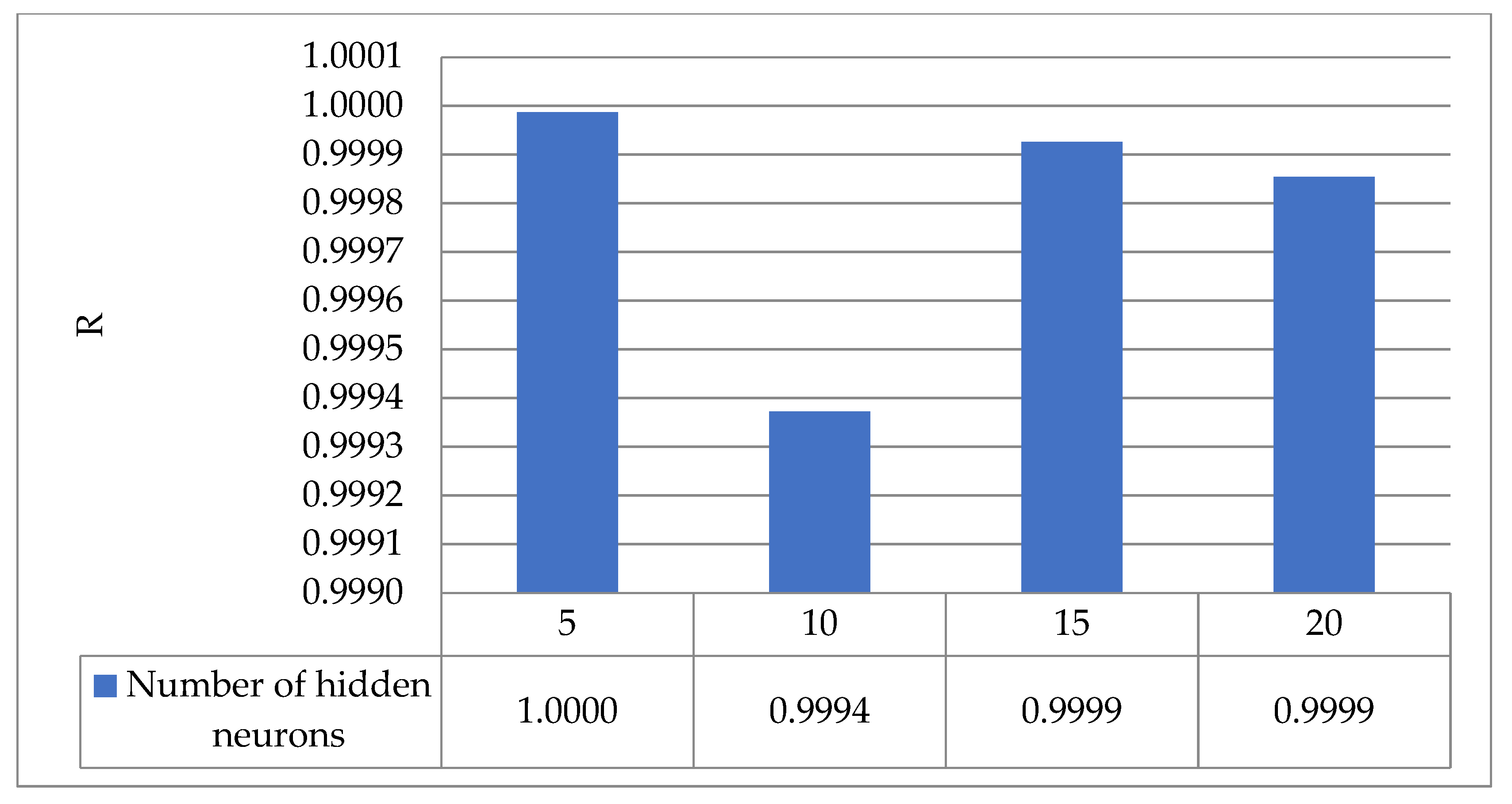
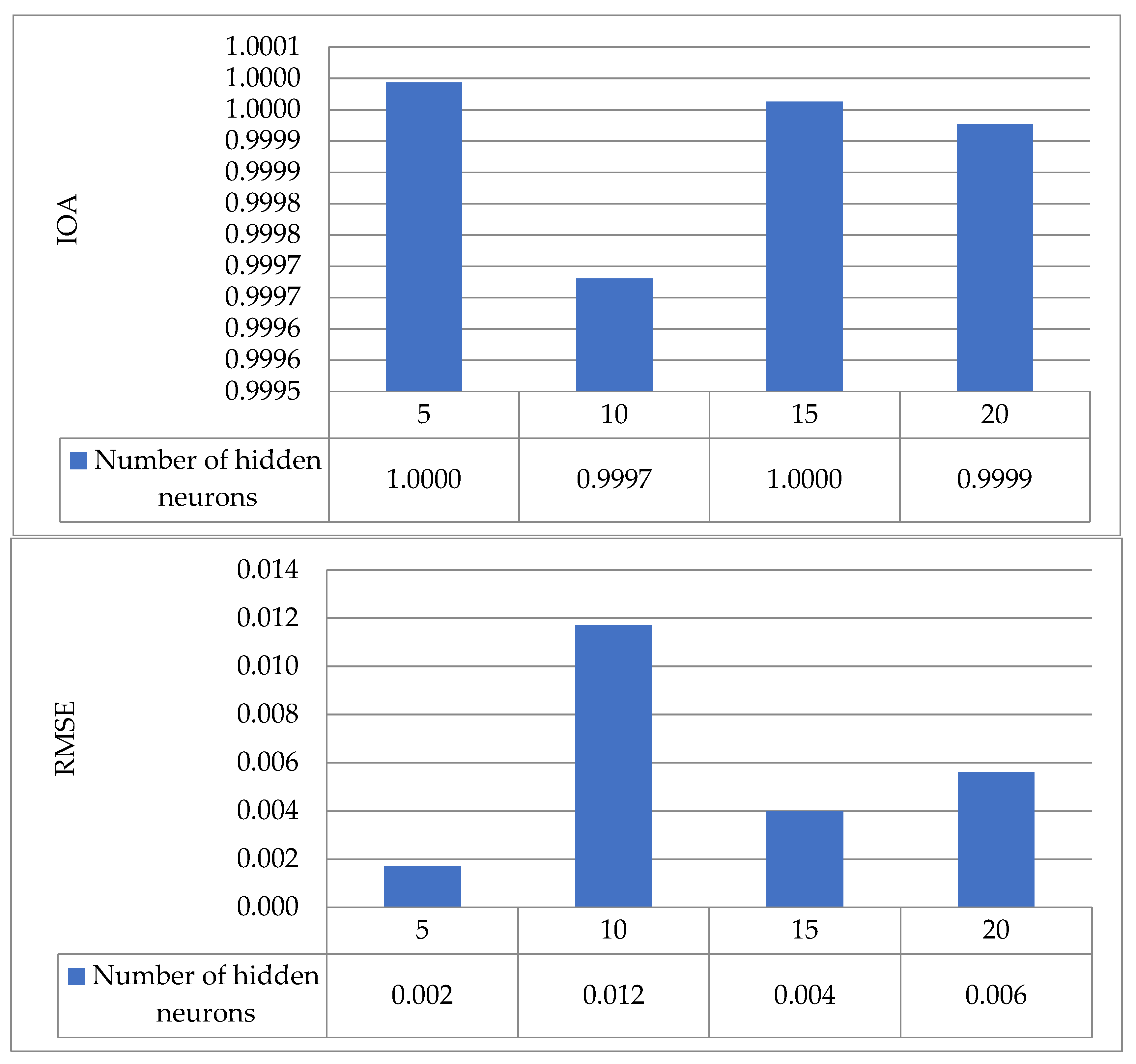
By trial and error, the optimum number of hidden neurons in each layer for the FFNN-TLBO model is determined. The number of hidden neurons is changed to 5, 10, 15, and 20. The prediction accuracy of the various topologies of the FFNN-TLBO model is assessed using various assessment criteria, as shown in Figure 8. Among all the assessed models, the network with five hidden neurons is associated with the best predicting accuracy. This network has the greatest R-value (i.e., 1.00), highest IOA value (i.e., 1.00), and the smallest RMSE value (i.e., 0.002). Therefore, to maximize the forecasting accuracy of the FFNN-TLBO model, it is recommended that the network parameters be adjusted to five hidden neurons.
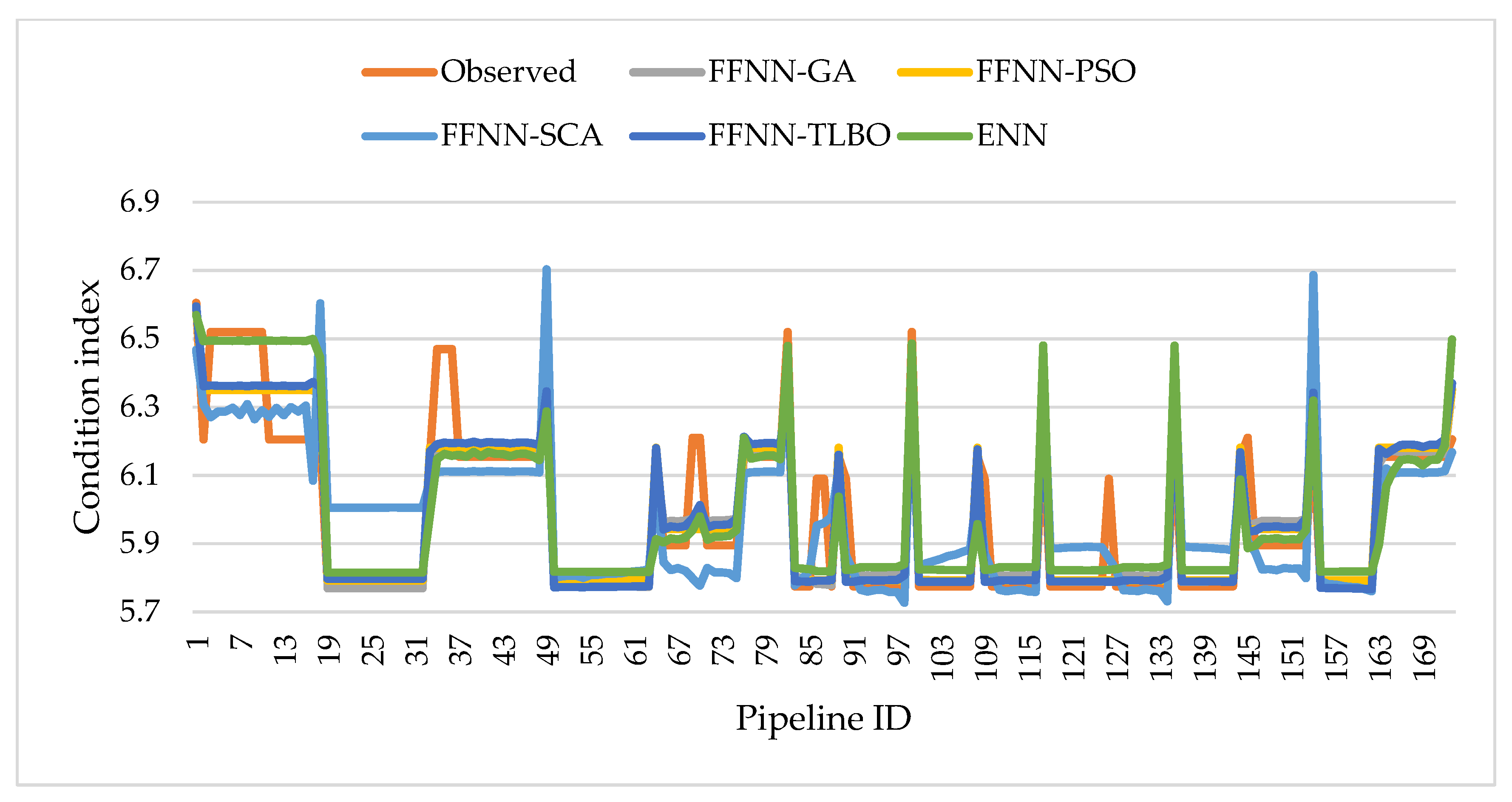
To test and validate the performance of the FFNN-TLBO model, the performance of the proposed model is examined against that of the ENN, FFNN-PSO, FFNN-GA, and FFNN-SCA models in the Shaker Al-Bahery network. Figure 9 compares the actual and predicted condition indices using established machine learning models. As shown in Table 7, the prediction models are assessed using three performance metrics (R, IOA, and RMSE). FFNN-TLBO has a value of 0.957 in the IOA measure, which is higher than the other models. The FFNN-TLBO model has an R-value of 0.928, compared to 0.896, 0.923, 0.927, and 0.837 for ENN, FFNN-GA, FFNN-PSO, and FFNN-SCA, respectively. Finally, the FFNN-TLBO model outperforms the other four models in terms of RMSE (0.095). This affirms that employing the TLBO algorithm to train FFNN improves the model’s prediction capabilities when compared to other forecasting models.
7. Conclusions
Most water pipes experience major degradation and deterioration problems. Therefore, it is of the utmost importance to estimate the condition of water pipes in order to implement the corrective action plans at the appropriate time to avoid catastrophic failures. This research examined the condition of water pipes using the Elman neural network (ENN) and feed-forward neural network (FFNN) coupled with genetic algorithms (GA), particle swarm optimization (PSO), sine cosine algorithm (SCA), and teaching-learning-based optimization (TLBO) algorithms. This study contributed to the literature by providing examples of using four algorithms to improve neural network performance and their application in the field of water supply pipe condition assessment. The proposed framework was validated using two water distribution networks in Shattora and Shaker Al-Bahery, Egypt. The inputs to these models in the Shattora network were pipe length, wall thickness, diameter, material, lining and coating, surface type, traffic distribution, cathodic protection, flow velocity, and c-factor. For the Shaker Al-Bahery network, the input data included length, diameter, and wall thickness. The prediction models were assessed using three criteria: index of agreement (IOA), correlation coefficient (R), and root mean squared error (RMSE).
For the Shattora network, it was found that the FFNN-PSO model (R = 0.993, IOA = 0.997, and RMSE = 0.038) outperformed the FFNN-GA model (R = 0.939, IOA = 0.968, and RMSE = 0.113) and ENN model (R = 0.987, IOA = 0.993, and RMSE = 0.054). Meanwhile, the FFNN model coupled with the SCA algorithm was associated with the worst performance evaluation metrics (i.e., R = 0.924, IOA = 0.952, and RMSE = 0.144). Finally, combining the FFNN with the TLBO algorithm (R = 0.999, IOA = 1.000, and RMSE = 0.012) improved the performance metrics in comparison with the other models. The R-value of the predicted data using FFNN-TLBO was higher than that of the FFNN-GA, FFNN-PSO, FFNN-SCA, and ENN models by 6.44%, 0.60%, 8.16%, and 1.30%, respectively. As for IOA, the forecasted data using FFNN-TLBO were higher than that of the FFNN-GA, FFNN-PSO, FFNN-SCA, and ENN models by 3.30%, 0.30%, 5.04%, and 0.66%, respectively. Furthermore, the RMSE of the predicted data using FFNN-TLBO was less than that of the FFNN-GA, FFNN-PSO, FFNN-SCA, and ENN models by 89.64%, 68.92%, 91.85%, and 78.48%, respectively. Furthermore, the RMSE of the FFNN-TLBO model was found to be less than that which was reported in the literature. Therefore, it can be concluded that the FFNN-TLBO model outperformed the other developed models and enhanced the accuracy of modeling the condition of water pipelines.
The optimum number of hidden neurons in each layer for the FFNN-TLBO model was determined by trial and error. The number of hidden neurons was changed to 5, 10, 15, and 20. The results confirmed that the network with five hidden neurons had the greatest R-value (i.e., 1.00), highest IOA value (i.e., 1.00), and the smallest RMSE value (i.e., 0.002). As a result, it was advised to adjust the number of hidden neurons to five in order to maximize the forecasting accuracy of the FFNN-TLBO model.
The performance of the FFNN-TLBO model was compared to that of the ENN, FFNN-PSO, FFNN-GA, and FFNN-SCA models to test and validate its performance in the Shaker Al-Bahery network. The IOA value for FFNN-TLBO was 0.957, which was greater than the other models. The R-value for the FFNN-TLBO model was 0.928, compared to 0.896, 0.923, 0.927, and 0.837 for the ENN, FFNN-GA, FFNN-PSO, and FFNN-SCA models. Finally, in terms of RMSE, the FFNN-TLBO model (0.095) outperformed the other four models. It can be concluded that applying the TLBO algorithm to train FFNN improved the model’s prediction abilities. Integrating neural networks and optimization algorithms improved the capacity of neural networks to address real-world problems while avoiding overfitting and local minima during training. The basic concept of the proposed FFNN-TLBO model is to take full advantage of FFNN’s strong global search ability and TLBO’s quick convergence. As a result, it has the ability to tackle a variety of optimization challenges. The good results obtained with this methodology could be an incentive for water companies to record quality and accurate data of the condition of the network pipes. This study was supposed to help the water municipality allocate its budget more accurately and effectively, as well as schedule the required intervention strategies. As for the study limitations, the data splitting approach for training and testing purposes could be addressed by applying cross-validation in future studies. This aids in providing a fair comparison of the performance of the developed models, particularly in addressing underfitting and overfitting.
Author Contributions
Conceptualization, N.E. and E.M.A.; methodology, N.E. and E.M.A.; formal analysis, N.E., E.M.A., A.A.-S. and G.A.; data curation, N.E., E.M.A., A.A.-S. and G.A.; investigation, N.E., E.M.A., A.A.-S. and G.A.; resources, N.E., E.M.A., A.A.-S. and G.A.; writing—original draft preparation, N.E., E.M.A., A.A.-S. and G.A.; writing—review and editing, N.E., E.M.A., A.A.-S. and G.A. All authors have read and agreed to the published version of the manuscript.
Funding
This research received no external funding.
Institutional Review Board Statement
Not applicable.
Informed Consent Statement
Informed consent was obtained from all subjects involved in the study.
Data Availability Statement
Some or all data, models, or code that support the findings of this study are available from the corresponding author upon reasonable request.
Conflicts of Interest
The authors declare no conflict of interest.
References
- Marzouk, M.; Hamid, S.A.; El-Said, M. A methodology for prioritizing water mains rehabilitation in Egypt. HBRC J. 2015, 11, 114–128. [Google Scholar] [CrossRef] [Green Version]
- Parvizsedghy, L.; Gkountis, I.; Senouci, A.; Zayed, T.; Alsharqawi, M.; El Chanati, H.; Mosleh, F. Deterioration assessment models for water pipelines. Int. J. Civ. Environ. Eng. 2017, 11, 1013–1022. [Google Scholar]
- Eliab, K. Modelling Pipe Failure Using Statistical Models. Ph.D Thesis, University of Nairobi, Nairobi, Kenya, 2015. [Google Scholar]
- Kakoudakis, K. Pipe Failure Prediction and Impacts Assessment in a Water Distribution Network. Ph.D Thesis, University of Exeter, Exeter, UK, 2019. [Google Scholar]
- Rajeev, P.; Kodikara, J.; Robert, D.; Zeman, P.; Rajani, B. Factors contributing to large diameter water pipe failure. West Afr. Monet. Inst. 2014, 10, 9–14. [Google Scholar]
- Rezaei, H.; Ryan, B.; Stoianov, I. Pipe failure analysis and impact of dynamic hydraulic conditions in water supply networks. Procedia Eng. 2015, 119, 253–262. [Google Scholar] [CrossRef] [Green Version]
- Bruaset, S.; Sægrov, S. An analysis of the potential impact of climate change on the structural reliability of drinking water pipes in cold climate regions. Water 2018, 10, 411. [Google Scholar] [CrossRef] [Green Version]
- Dawood, T.; Elwakil, E.; Novoa, H.M.; Delgado, J.F.G. Pressure data-driven model for failure prediction of PVC pipelines. Eng. Fail. Anal. 2020, 116, 104769. [Google Scholar] [CrossRef]
- Harvey, R.; McBean, E.A.; Gharabaghi, B. Predicting the timing of water main failure using artificial neural networks. J. Water Resour. Plan. Manag. 2014, 140, 425–434. [Google Scholar] [CrossRef]
- AWWA (American Water Works Association). Buried No Longer: Confronting America’s Water Infrastructure Challenge; AWWA: Denver, CO, USA, 2012. [Google Scholar]
- ASCE (American Society of Civil Engineers). Infrastructure Report Card. Available online: https://infrastructurereportcard.org/ (accessed on 15 August 2021).
- Folkman, S. Water Main Break Rates in the USA and Canada: A Comprehensive Study. Available online: https://digitalcommons.usu.edu/mae_facpub/174/ (accessed on 11 August 2021).
- CIRC (Canadian Infrastructure Report Card 2019). Monitoring the State of Canada’s Core Public Infrastructure. Available online: http://canadianinfrastructure.ca/downloads/canadian-infrastructure-report-card-2019.pdf (accessed on 12 August 2021).
- Hussein, H.; Lambert, L.A. A Rentier state under blockade: Qatar’s water-energy-food predicament from energy abundance and food insecurity to a silent water crisis. Water 2020, 12, 1051. [Google Scholar] [CrossRef] [Green Version]
- See, K.F.; Ma, Z. Does non-revenue water affect Malaysia’s water services industry productivity? Util. Policy 2018, 54, 125–131. [Google Scholar] [CrossRef]
- EcoMENA. Egypt’s Water Crisis—Recipe For Disaster. Available online: https://www.ecomena.org/egypt-water/ (accessed on 10 September 2021).
- Wadie, M.; Mahmoud, N. CAPMAS: Egypt’s Pure Water Production Rises by 9.9%. Available online: http://see.news/capmas-egypts-pure-water-production-rises-by-9-9/ (accessed on 10 September 2021).
- Ayad, A.; Khalifa, A.; Fawy, M.E.; Moawad, A. An integrated approach for non-revenue water reduction in water distribution networks based on field activities, optimisation, and GIS applications. Ain Shams Eng. J. 2021, 12, 3509–3520. [Google Scholar] [CrossRef]
- Nassar, A. Egypt Plans to Face Water Scarcity, Allots LE 900B. Available online: http://www.egypttoday.com/Article/1/43824/Egypt-plans-to-face-water-scarcity-allots-LE-900B (accessed on 10 September 2021).
- Dridi, L.; Mailhot, A.; Parizeau, M.; Villeneuve, J.P. Multiobjective approach for pipe replacement based on Bayesian inference of break model parameters. J. Water Resour. Plan. Manag. 2009, 135, 344–354. [Google Scholar] [CrossRef]
- Faiz, R.B.; Edirisinghe, E.A. Decision making for predictive maintenance in asset information management. Interdiscip. J. Inf. Knowl. Manag. 2009, 4, 23–36. [Google Scholar]
- ICE (Institution of Civil Engineers). ICE’s Guiding Principles of Asset Management: Realizing a World Class Infrastructure. Available online: https://www.cices.org/content/uploads/2013/05/Guiding-Principles-of-Asset-Management-3.pdf (accessed on 10 September 2021).
- Røstum, J. Statistical Modelling of Water Pipe Failures in Water Networks. Ph.D Thesis, Norwegian University of Science and Technology, Trondheim, Norway, 2000. [Google Scholar]
- Kerwin, S.; Adey, B.T. Optimal Intervention Program Determination of a Water Distribution System. In Proceedings of the Leading Edge Sustainable Asset Management of Water and Wastewater Infrastructure Conference, Trondheim, Norway, 20–22 June 2017. [Google Scholar]
- Dawood, T.; Elwakil, E.; Novoa, H.M.; Delgado, J.F.G. Soft computing for modeling pipeline risk index under uncertainty. Eng. Fail. Anal. 2020, 117, 104949. [Google Scholar] [CrossRef]
- Dawood, T.; Elwakil, E.; Novoa, H.M.; Delgado, J.F.G. Artificial intelligence for the modeling of water pipes deterioration mechanisms. Autom. Constr. 2020, 120, 103398. [Google Scholar] [CrossRef]
- Misiunas, D.; Vitkovsky, J.; Olsson, G.; Simpson, A.; Lambert, M. Pipeline break detection using transient monitoring. J. Water Resour. Plan. Manag. 2005, 131, 316–325. [Google Scholar] [CrossRef] [Green Version]
- Covas, D.; Ramos, H. Case studies of leak detection and location in water pipe systems by inverse transient analysis. J. Water Resour. Plan. Manag. 2010, 136, 248–257. [Google Scholar] [CrossRef]
- Brunone, B.; Meniconi, S.; Capponi, C. Numerical analysis of the transient pressure damping in a single polymeric pipe with a leak. Urban Water J. 2018, 15, 760–768. [Google Scholar] [CrossRef]
- Meniconi, S.; Brunone, B.; Frisinghelli, M. On the role of minor branches, energy dissipation, and small defects in the transient response of transmission mains. Water 2018, 10, 187. [Google Scholar] [CrossRef] [Green Version]
- Meniconi, S.; Capponi, C.; Frisinghelli, M.; Brunone, B. Leak detection in a real transmission main through transient tests: Deeds and misdeeds. Water Resour. Res. 2021, 57, e2020WR027838. [Google Scholar] [CrossRef]
- Kim, K.; Seo, J.; Hyung, J.; Kim, T.; Kim, J.; Koo, J. Economic-based approach for predicting optimal water pipe renewal period based on risk and failure rate. Environ. Eng. Res. 2019, 24, 63–73. [Google Scholar] [CrossRef] [Green Version]
- Kim, S.; Jun, H.D.; Yoo, D.G.; Kim, J.H. A framework for improving reliability of water distribution systems based on a segment-based minimum cut-set approach. Water 2019, 11, 1524. [Google Scholar] [CrossRef] [Green Version]
- Nishiyama, M.; Filion, Y. Review of statistical water main break prediction models. Can. J. Civ. Eng. 2013, 40, 972–979. [Google Scholar] [CrossRef]
- Nemeth, L. A Comparison of Risk Assessment Models for Pipe Replacement and Rehabilitation in a Water Distribution System. MSc Thesis, California Polytechnic State University, San Luis Obispo, CA, USA, 2016. [Google Scholar]
- Cortez, H. A Risk Analysis Model for the Maintenance and Rehabilitation of Pipes in a Water Distribution System: A Statistical Approach. MSc Thesis, California Polytechnic State University, San Luis Obispo, CA, USA, 2015. [Google Scholar]
- Clark, R.M.; Stafford, C.L.; Goodrich, J.A. Water distribution systems: A spatial and cost evaluation. J. Water Resour. Plan. Manag. 1982, 108, 243–256. [Google Scholar] [CrossRef]
- Zangenehmadar, Z.; Moselhi, O. Assessment of remaining useful life of pipelines using different artificial neural networks models. J. Perform. Constr. Facil. 2016, 30, 04016032. [Google Scholar] [CrossRef]
- Elshaboury, N.; Marzouk, M. Comparing Machine Learning Models For Predicting Water Pipelines Condition. In Proceedings of the Second Novel Intelligent and Leading Emerging Sciences Conference (NILES), Giza, Egypt, 24–26 October 2020. [Google Scholar]
- Zhang, C.; Ye, Z. Water pipe failure prediction using AutoML. Facilities 2020, 39, 36–49. [Google Scholar] [CrossRef]
- Fan, X.; Zhang, X.; Yu, X.B. Machine learning model and strategy for fast and accurate detection of leaks in water supply network. J. Intellect. Prop. Rights 2021, 2, 1–21. [Google Scholar] [CrossRef]
- Jara-Arriagada, C.; Stoianov, I. Pipe breaks and estimating the impact of pressure control in water supply networks. Reliab. Eng. Syst. Saf. 2021, 210, 107525. [Google Scholar] [CrossRef]
- Martínez García, D.; Lee, J.; Keck, J. Drinking water pipeline failure analysis based on spatiotemporal clustering and Poisson regression. J. Pipeline Syst. Eng. Pract. 2021, 12, 05020006. [Google Scholar] [CrossRef]
- Ravichandran, T.; Gavahi, K.; Ponnambalam, K.; Burtea, V.; Mousavi, S.J. Ensemble-based machine learning approach for improved leak detection in water mains. J. Hydroinformatics 2021, 23, 307–323. [Google Scholar] [CrossRef]
- Awe, O.M.; Okolie, S.T.A.; Fayomi, O.S.I. Analysis and optimization of water distribution systems: A case study of Kurudu post service housing estate, Abuja, Nigeria. Results Eng. 2020, 5, 100100. [Google Scholar] [CrossRef]
- Elshaboury, N.; Attia, T.; Marzouk, M. Application of evolutionary optimization algorithms for rehabilitation of water distribution networks. J. Constr. Eng. Manag. 2020, 146, 04020069. [Google Scholar] [CrossRef]
- Elshaboury, N.; Abdelkader, E.; Marzouk, M. Application of Modified Invasive Weed Algorithm for Condition-Based Budget Allocation of Water Distribution Networks. In Design and Construction of Smart Cities: Toward Sustainable Community; Springer: Cham, Switzerland, 2021; pp. 121–131. [Google Scholar]
- Elman, J.L. Finding structure in time. Cogn. Sci. 1990, 14, 179–211. [Google Scholar] [CrossRef]
- Zou, J.; Han, Y.; So, S.S. Overview of artificial neural networks. Methods Mol. Biol. 2009, 458, 14–22. [Google Scholar]
- Fahmy, M.; Moselhi, O. Automated detection and location of leaks in water mains using infrared photography. J. Perform. Constr. Fac. 2009, 24, 242–248. [Google Scholar] [CrossRef]
- Sbarufatti, C.; Corbetta, M.; Manes, A.; Giglio, M. Sequential monte-carlo sampling based on a committee of artificial neural networks for posterior state estimation and residual lifetime prediction. Int. J. Fatigue 2016, 83, 10–23. [Google Scholar] [CrossRef]
- Golnaraghi, S.; Zangenehmadar, Z.; Moselhi, O.; Alkass, S. Application of artificial neural network(s) in predicting formwork labour productivity. Adv. Civ. Eng. 2019, 2019, 5972620. [Google Scholar] [CrossRef] [Green Version]
- Firat, M.; Gungor, M. Generalized regression neural networks and feed forward neural networks for prediction of scour depth around bridge piers. Adv. Eng. Softw. 2009, 40, 731–737. [Google Scholar] [CrossRef]
- Holland, J. Adaptation in Natural and Artificial Systems; University of Michigan Press: Ann Arbor, MI, USA, 1975. [Google Scholar]
- Eberhart, R.C.; Kennedy, J. A New Optimizer Using Particle Swarm Theory. In Proceeding of the Sixth International Symposium on Micro Machine and Human Science, Nagoya, Japan, 4–6 October 1995; pp. 39–43. [Google Scholar]
- Shi, Y.; Eberhart, R. Parameter Selection in Particle Swarm Optimization. In International Conference on Evolutionary Programming; Springer: London, UK, 1998. [Google Scholar]
- Mirjalili, S. SCA: A sine cosine algorithm for solving optimization problems. Knowl. Based Syst. 2016, 96, 120–133. [Google Scholar] [CrossRef]
- Abualigah, L.; Diabat, A. Advances in sine cosine algorithm: A comprehensive survey. Artif. Intell. Rev. 2021, 54, 2567–2608. [Google Scholar] [CrossRef]
- Rao, R.V.; Savsani, V.J.; Vakharia, D.P. Teaching–learning-based optimization: A novel method for constrained mechanical design optimization problems. Comput. Aided Des. 2011, 43, 303–315. [Google Scholar] [CrossRef]
- Chen, Y.K.; Weng, S.X.; Liu, T.P. Teaching-learning based optimization (TLBO) with variable neighborhood search to retail shelf-space allocation. Mathematics 2020, 8, 1296. [Google Scholar] [CrossRef]
- Mohanty, B.; Tripathy, S. A teaching learning based optimization technique for optimal location and size of DG in distribution network. J. Electr. Syst. Inf. Technol. 2016, 3, 33–44. [Google Scholar] [CrossRef] [Green Version]
- Yaseen, Z.M.; Ghareb, M.I.; Ebtehaj, I.; Bonakdari, H.; Siddique, R.; Heddam, S.; Yusif, A.; Deo, R. Rainfall pattern forecasting using novel hybrid intelligent model based ANFIS-FFA. Water Resour. Manag. 2017, 32, 105–122. [Google Scholar] [CrossRef]
- Abd Rahman, N.; Muhammad, N.S.; Abdullah, J.; Wan Mohtar, W.H.M. Model performance indicator of aging pipes in a domestic water supply distribution network. Water 2019, 11, 2378. [Google Scholar] [CrossRef] [Green Version]
- Aydogdu, M.; Firat, M. Estimation of failure rate in water distribution network using fuzzy clustering and LS-SVM methods. Water Resour. Manag. 2014, 29, 1575–1590. [Google Scholar] [CrossRef]
- El-Abbasy, M.; El-Chanati, H.; Mosleh, F.; Senouci, A.; Zayed, T.; Al-Derham, H. Integrated performance assessment model for water distribution networks. Struct. Infrastruct. E. 2016, 12, 1505–1524. [Google Scholar] [CrossRef]
- Saaty, T.L. A scaling method for priorities in a hierarchical structure. J. Math. Psychol. 1977, 15, 234–281. [Google Scholar] [CrossRef]
- Fares, H. Evaluating the Risk of Water Main Failure Using a Hierarchical Fuzzy Expert System. MSc Thesis, Concordia University, Montreal, QC, Canada, 2008. [Google Scholar]
- Elshaboury, N.; Attia, T.; Marzouk, M. Reliability assessment of water distribution networks using minimum cut set analysis. J. Infrastruct. Syst. 2021, 27, 04020048. [Google Scholar] [CrossRef]
- Devikanniga, D.; Vetrivel, K.; Badrinath, N. Review of meta-heuristic optimization based artificial neural networks and its applications. J. Phys. Conf. Ser. 2019, 1362, 012074. [Google Scholar] [CrossRef]
- Mirjalili, S.; Hashim, S.Z.M.; Sardroudi, H.M. Training feedforward neural networks using hybrid particle swarm optimization and gravitational search algorithm. Appl. Math. Comput. 2012, 218, 11125–11137. [Google Scholar] [CrossRef]
- Pater, L. Application of artificial neural networks and genetic algorithms for crude fractional distillation process modeling. arXiv 2016, arXiv:1605.00097. [Google Scholar]
- Lazzús, J.A. Neural network-particle swarm modeling to predict thermal properties. Math Comput. Model 2013, 57, 2408–2418. [Google Scholar] [CrossRef]
- Senior Consulting Engineers Office. Report: Design of the Water Network in Shattora Region; Senior Consulting Engineers Office: Cairo, Egypt, 2018. [Google Scholar]
- HBRC (Housing and Building National Research Center). Egyptian Code for Design and Implementation of Pipelines for Drinking Water and Sewage Networks; HBRC: Giza, Egypt, 2010. [Google Scholar]
- Mahmoodabadi, M.J.; Ostadzadeh, R. CTLBO: Converged teaching-learning-based optimization. Cogent Eng. 2019, 6, 1654207. [Google Scholar] [CrossRef]
Figure 1.
ENN architecture.

Figure 2.
FFNN architecture.

Figure 3.
Flowchart for developing a condition prediction model.

Figure 4.
Flowchart of neural network model procedure.

Figure 5.
Water network layout in (a) Shattora and (b) Shaker Al-Bahery.

Figure 6.
Boxplots of the performance of machine learning models in the Shattora network.

Figure 7.
Line plots of the observed and anticipated condition indices in the Shattora network.

Figure 8.
Criteria for testing alternative FFNN-TLBO models.


Figure 9.
Line plots of the observed and predicted condition indices in the Shaker Al-Bahery network.
Figure 9.
Line plots of the observed and predicted condition indices in the Shaker Al-Bahery network.


Table 1.
Sample of the input and output factors in the Shattora network.
| ID | Length | Material | Diameter | Thickness | Lining and Coating | Surface Type | Traffic Distribution | Flow Velocity | Cathodic Protection | C-Factor | Condition Index |
|---|---|---|---|---|---|---|---|---|---|---|---|
| 1 | 150 | 1 | 400 | 43 | 0 | 1 | 2 | 0.07 | 1 | 140 | 6.40 |
| 2 | 2000 | 2 | 700 | 174 | 1 | 1 | 3 | 0.75 | 0 | 120 | 6.76 |
| 3 | 479 | 3 | 500 | 74.8 | 0 | 1 | 3 | 1.27 | 1 | 120 | 6.29 |
| 4 | 150 | 2 | 600 | 174 | 1 | 1 | 3 | 0.14 | 0 | 120 | 6.76 |
| 5 | 2100 | 2 | 1200 | 244 | 1 | 1 | 3 | 1.06 | 0 | 120 | 6.76 |
Table 2.
Statistical parameters of quantitative input and output parameters for condition prediction in the Shattora network.
Table 2.
Statistical parameters of quantitative input and output parameters for condition prediction in the Shattora network.
| Variable | Mean | Median | Maximum | Minimum | Standard Deviation | Kurtosis | Skewness |
|---|---|---|---|---|---|---|---|
| Length | 1319.28 | 817.00 | 6100.00 | 2.00 | 1407.07 | 1.52 | 1.44 |
| Diameter | 461.11 | 400.00 | 1200.00 | 200.00 | 270.65 | 1.46 | 1.47 |
| Thickness | 76.34 | 43.00 | 244.00 | 21.60 | 71.20 | 0.16 | 1.28 |
| Flow velocity | 0.68 | 0.39 | 6.92 | 0.00 | 0.94 | 25.85 | 4.53 |
| Condition index | 135.31 | 140.00 | 140.00 | 120.00 | 8.53 | −0.38 | −1.28 |
Table 3.
Sample of the input and output factors in the Shaker Al-Bahery network.
| ID | Length | Diameter | Thickness | Condition Index |
|---|---|---|---|---|
| 1 | 80.72 | 400 | 43 | 6.61 |
| 2 | 32.37 | 300 | 30 | 6.21 |
| 3 | 27.04 | 300 | 30 | 6.52 |
| 4 | 100.03 | 100 | 10.6 | 5.78 |
| 5 | 34.88 | 200 | 21.6 | 6.47 |
Table 4.
Statistical parameters of input and output parameters for condition prediction in the Shaker Al-Bahery network.
Table 4.
Statistical parameters of input and output parameters for condition prediction in the Shaker Al-Bahery network.
| Variable | Mean | Median | Maximum | Minimum | Standard Deviation | Kurtosis | Skewness |
|---|---|---|---|---|---|---|---|
| Length | 64.0 | 46.6 | 169.4 | 5.0 | 46.0 | 0.2 | 1.3 |
| Diameter | 156.1 | 100.0 | 400.0 | 100.0 | 73.0 | 0.1 | 1.1 |
| Thickness | 16.3 | 10.6 | 43.0 | 10.6 | 7.3 | 0.0 | 1.0 |
| Condition index | 6.0 | 5.8 | 6.6 | 5.8 | 0.2 | −0.3 | 0.9 |
Table 5.
Statistics on the results of the neural network models in the Shattora network.
| Statistic Measure | Observed | Optimized Neural Network Models | ENN | |||
|---|---|---|---|---|---|---|
| FFNN-GA | FFNN-PSO | FFNN-SCA | FFNN-TLBO | |||
| Mean | 6.25 | 6.25 | 6.25 | 6.18 | 6.25 | 6.24 |
| Median | 6.29 | 6.13 | 6.33 | 6.05 | 6.26 | 6.00 |
| Standard deviation | 0.33 | 0.31 | 0.33 | 0.33 | 0.33 | 0.33 |
Table 6.
Performance measures of the neural network models in the Shattora network.
| Performance Measure | Optimized Neural Network Models | ENN | |||
|---|---|---|---|---|---|
| FFNN-GA | FFNN-PSO | FFNN-SCA | FFNN-TLBO | ||
| IOA | 0.968 | 0.997 | 0.952 | 1.000 | 0.993 |
| R | 0.939 | 0.993 | 0.924 | 0.999 | 0.987 |
| RMSE | 0.113 | 0.038 | 0.144 | 0.012 | 0.054 |
Table 7.
Performance measures of the neural network models in the Shaker Al-Bahery network.
| Performance Measure | Optimized Neural Network Models | ENN | |||
|---|---|---|---|---|---|
| FFNN-GA | FFNN-PSO | FFNN-SCA | FFNN-TLBO | ||
| IOA | 0.953 | 0.955 | 0.894 | 0.957 | 0.937 |
| R | 0.923 | 0.927 | 0.837 | 0.928 | 0.896 |
| RMSE | 0.098 | 0.096 | 0.139 | 0.095 | 0.117 |
Publisher’s Note: MDPI stays neutral with regard to jurisdictional claims in published maps and institutional affiliations. |
© 2021 by the authors. Licensee MDPI, Basel, Switzerland. This article is an open access article distributed under the terms and conditions of the Creative Commons Attribution (CC BY) license (https://creativecommons.org/licenses/by/4.0/).
Share and Cite
MDPI and ACS Style
Elshaboury, N.; Abdelkader, E.M.; Al-Sakkaf, A.; Alfalah, G. Teaching-Learning-Based Optimization of Neural Networks for Water Supply Pipe Condition Prediction. Water 2021, 13, 3546. https://doi.org/10.3390/w13243546
AMA Style
Elshaboury N, Abdelkader EM, Al-Sakkaf A, Alfalah G. Teaching-Learning-Based Optimization of Neural Networks for Water Supply Pipe Condition Prediction. Water. 2021; 13(24):3546. https://doi.org/10.3390/w13243546
Chicago/Turabian StyleElshaboury, Nehal, Eslam Mohammed Abdelkader, Abobakr Al-Sakkaf, and Ghasan Alfalah. 2021. "Teaching-Learning-Based Optimization of Neural Networks for Water Supply Pipe Condition Prediction" Water 13, no. 24: 3546. https://doi.org/10.3390/w13243546
Note that from the first issue of 2016, this journal uses article numbers instead of page numbers. See further details here.