Hydrological Modeling of Karst Watershed Containing Subterranean River Using a Modified SWAT Model: A Case Study of the Daotian River Basin, Southwest China

Abstract

Karst watershed refers to the total range of surface and underground recharge areas of rivers (including subterranean rivers and surface rivers) in karst areas. Karst water resources, as the primary source of domestic water supply in southwest China, are vital for the social and economic development of these regions. It is greatly significant to establish a high-precision hydrological model of karst watershed for guiding water resources management in karst areas. Choosing the Daotian river basin in the Wumeng Mountains of Southwest China as the study area, this paper proposed a method for simplifying karst subterranean rivers into surface rivers by modifying the digital elevation model (DEM) based on a field survey and tracer test. This method aims to solve the inconsistency between the topographical drainage divides and actual catchment boundaries in karst areas. The Soil and Water Assessment Tool (SWAT) model was modified by replacing the single-reservoir model in the groundwater module with a three-reservoir model to depict the constraints of multiple media on groundwater discharge in the karst system. The results show that the catchment areas beyond topographic watershed were effectively identified after simplifying subterranean rivers to surface rivers based on the modified DEM data, which ensured the accuracy of the basic model. For the calibration and two validation periods, the Nash–Sutcliffe efficiencies (NSE) of the modified SWAT model were 0.87, 0.83, and 0.85, respectively, and R² were 0.88, 0.84, and 0.86, respectively. The NSE of the modified SWAT model was 0.09 higher than that of the original SWAT model in simulating baseflow, which effectively improved the simulation accuracy of daily runoff. In addition, the modified SWAT model had a lower uncertainty within the same parameter ranges than the original one. Therefore, the modified SWAT model is more applicable to karst watersheds.

1. Introduction

Karst groundwater is the main source of domestic water supply for about 25% of the world’s population [1], and it is of great significance for guiding water resources management in karst areas, in order to establish a high-precision hydrological model of karst watersheds. However, the karst aquifers show a strong heterogeneity due to karstification [2,3], and there is a duality in karst aquifers recharge, runoff, and discharge [4,5,6], leading to a very complicated karst hydrological cycle process. Furthermore, the surface drainage divides tend to be inconsistent with underground drainage divides in karst areas [7,8,9]. All of these aspects pose great challenges to the hydrological modeling of karst watersheds.

The hydrological models of watersheds can be grouped into lumped, semi-distributed, and distributed categories. It is a compromised solution to model karst watersheds using a semi-distributed hydrological model [10], which not only takes account the spatial differences in soil, terrain, and land use [11], but also overcomes the difficulty with the obtainment of the structure and hydraulic parameters of karst aquifers. The Soil and Water Assessment Tool (SWAT) model is a semi-distributed hydrological model with open-source code [12,13] and was widely and successfully tested in various watersheds on different scales around the world [14,15,16,17,18]. However, there are very limited studies on the application of the SWAT model in karst watersheds [19,20,21]. In the SWAT model, a single, linear reservoir model is adopted to calculate the discharge of groundwater into river channels, and the groundwater recharge only incorporates the infiltration of soil water [22]. However, aside from the infiltration of soil water, the groundwater recharge in karst areas also includes the intensive and rapid recharge from sinkholes, ponors, and fissures [23]. In addition, the discharge process of karst groundwater is nonlinear due to the effects of multiple media [24,25,26]. Therefore, it underestimates groundwater recharge needed to use the SWAT model in the simulation of the hydrological process in karst watersheds [21,27,28,29], leading to unsatisfactory simulation results of the runoff in low-flow periods.

To improve the simulation accuracy and adaptability of karst watersheds using the SWAT model, previous studies improved the groundwater module in the SWAT model in different ways. In terms of karst groundwater recharge, some researchers described the rapid recharge from karst aquifers by using ponds [10], wetlands [30], or hydrological response units (HRUs) [31] to represent sinkholes, thus effectively increasing groundwater recharge. Some studies simulated the amount of water injected from sinkholes by practically investigating the scale of sinkholes above riverbeds and modifying the algorithm of groundwater recharge, thus successfully reproducing the hydrological curves observed [32]. Regarding the description of karst groundwater discharge, some researchers considered the differences between the fracture water in karst aquifers and flow in karst conduits, and thus replaced the single-reservoir model in the SWAT model with a dual-reservoir model [30,33,34]. As a result, the hydrological conditions of karst watersheds could be simulated in a more detailed way. However, the effects of epikarst zones on the groundwater discharge process were ignored.

Wang et al. [35] proposed a three-reservoir model method coupled with the SWAT model to describe the constraints of epikarst, karst conduits, and fractures in karst aquifers on groundwater. Compared with the single-reservoir and the dual-reservoir model, this three-reservoir model method can not only describe the rapid flow and the slow flow in karst system, but also add the regulation and storage function of epikarst zone. Although the three-reservoir model improved the performance of SWAT in karst watershed, it has shortcomings in describing the rapid recharge of the karst system. The rapid recharge of the three-reservoir model was added to the epikarst zone instead of directly entering the rapid flow system, which weakened the rapid recharge process [35]. The SWAT algorithm was also modified in some studies to model karst watersheds where the topographic drainage divides are inconsistent with the actual catchment boundaries [9,36]. However, these improved methods are suitable for modeling interbasin groundwater flow in karst areas, and they have limitations in watersheds containing karst subterranean rivers. The reason is that the flow characteristics of subterranean rivers are similar to surface rivers. The combination of hydrological methods with hydrogeological methods is critical to the hydrological modeling of karst watersheds [37]. Meanwhile, the modeling using the SWAT model based on field surveys and tracer tests [21] can effectively ensure the correct identification of actual catchment boundaries in karst watersheds. Overall, the key to the hydrological modeling of karst watersheds using the SWAT model is the correct identification of catchment boundaries and the reasonable characterization of the karst water cycle process.

Focusing on the karst watersheds in the Wumeng Mountains area in Southwest China, the purposes of this study are to improve the adaptability of the SWAT model in the karst watersheds containing subterranean rivers, and to more accurately simulate the contribution made by daily baseflow to the rivers in karst watersheds. The main objective of this study is to solve the inconsistency between the topographical drainage divides and actual catchment boundaries in karst areas using coupled tracing test techniques to a semi-distributed hydrological model (SWAT). In addition, a three-reservoir model is used to describe the constraints of multiple media on groundwater discharge in the karst aquifer, instead of a single reservoir in the SWAT model.

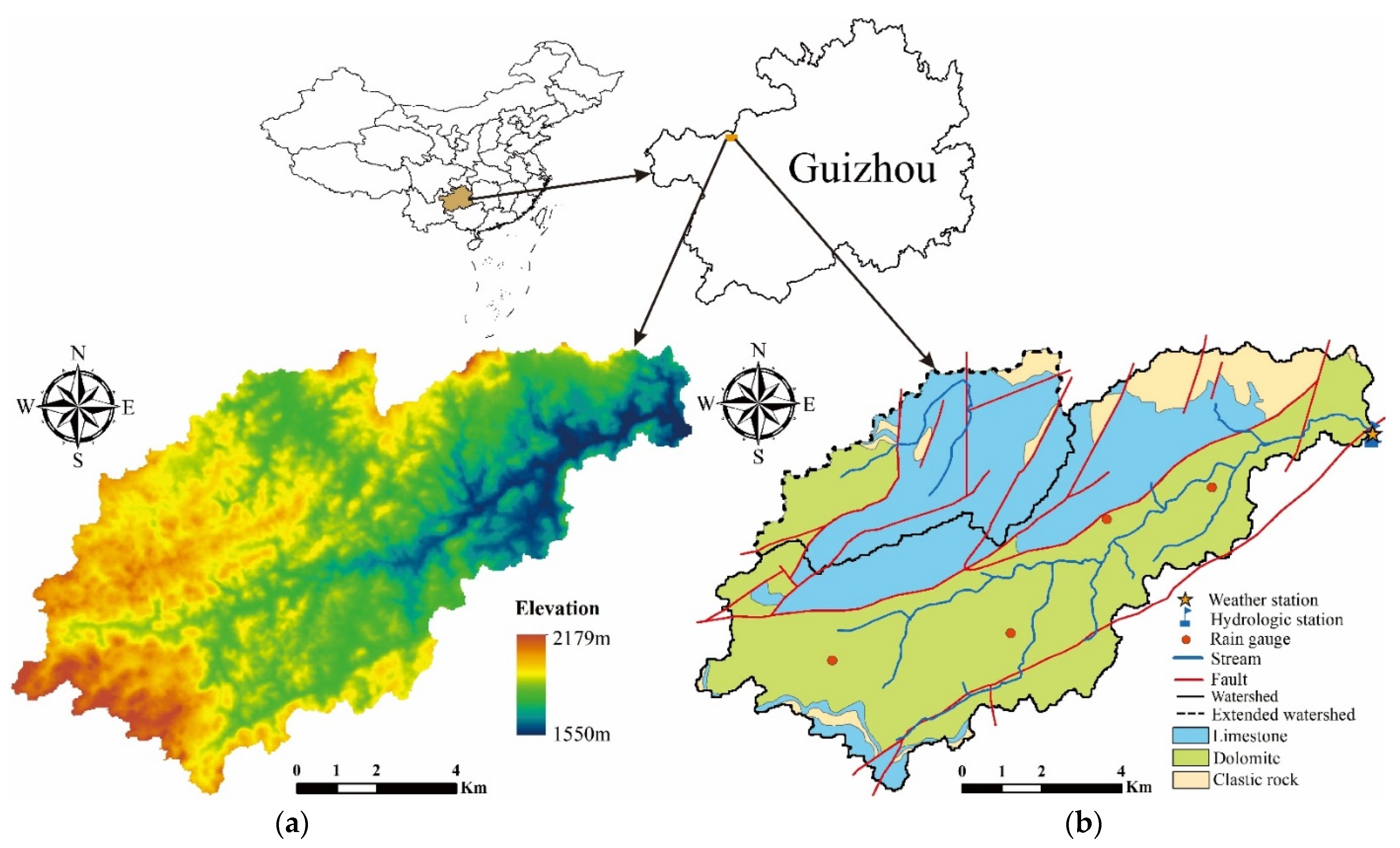
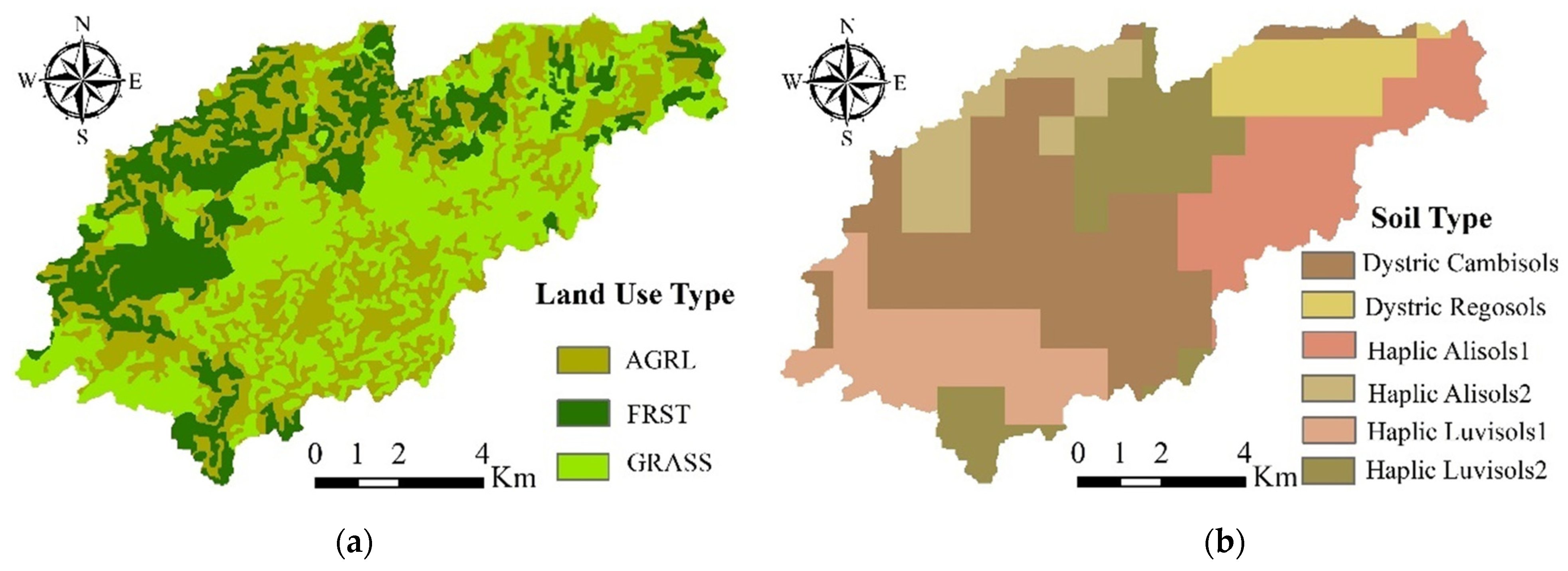
2. Watershed Description

The Daotian River watershed is located in Qixingguan District, Bijie City, Guizhou Province, China, covering a total area of 99.21 km². It lies in the hinterland of the Wumeng Mountains and in the upper reaches of the Baifu River, a tributary of Wujiang River system. It is high in the southwest and low in the northeast, with an elevation of 1550–2179 m (Figure 1a); the river flows from southwest to northeast (Figure 1b). The Daotian River watershed has a temperate monsoon climate, with an average multiyear temperature of 13.8 °C and average multiyear precipitation of 910.84 mm.

The strata in the Daotian River watershed are mainly composed of carbonates (Figure 1b), including 53.44% dolomite, 38.05% limestones, and 8.51% clastic rocks, and the Daotian River watershed is a typical small karst watershed. The faults in the watershed are dominated by reverse faults with poor hydraulic conductivity. In terms of landform, the Daotian River watershed mainly consists of hills, depressions, and karst troughs and valleys. In the distribution area of limestone, karst morphologies such as sinkholes and ponors occur on the ground surface, and highly networked karst conduits with high hydraulic conductivity are distributed underground. Surface streams mainly develop in the distribution area of dolomites but do not develop in the distribution area of limestone.

Due to the effects of karst development characteristics, the actual catchment boundaries are inconsistent with the surface drainage divides in the Daotian River watershed. Beyond the topographic drainage divides in the limestone distribution area in the northwestern part of the watershed, the water from an area of 24.75 km² is discharged into the watershed through underground conduits (Figure 1b). The groundwater in the watershed is recharged through infiltration and concentrated recharge and discharges into river channels in the form of springs or subterranean rivers. There are four rain-gauging stations evenly distributed along the river development direction in the Daotian River watershed (Figure 1b). Furthermore, one hydrological and one weather station were located at the outlet of the watershed, and provided sufficient daily meteorological and streamflow data for this study.

3. Methodology

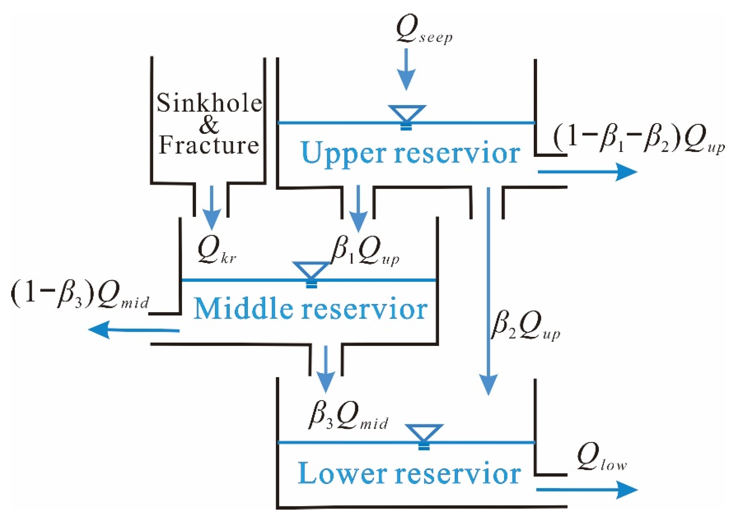
3.1. Model Description and Modifications

SWAT is a continuous-time, physical-process-based, and semi-distributed model. It can automatically generate a river network according to topographic data, generate sub-watersheds according to the river network density and the positions of monitoring points, and divide the sub-watersheds into HRUs based on land use/cover, soil, and slope to calculate runoff yield and concentration [22]. The principle of SWAT is the water balance equation:

$$S{W}_t=S{W}_0+{\displaystyle \sum }_{t=1}^t\left(R_i-Q_i-E{T}_i-W_i-Q{R}_i\right)$$

(1)

where SW_t is the final soil water content (mm), SW₀ is the initial soil water content (mm), R_i is the amount of precipitation on day i (mm), Q_i is the amount of surface runoff on day i (mm), ET_i is the amount of evapotranspiration on day i (mm), W_i is the amount of seepage on day i (mm), QR_i is the amount of return flow on day i (mm), and i is the time (day).

Given that the original SWAT groundwater module has shortcomings in describing the characteristics of the rapid recharge and discharge of karst groundwater, this study improves the three-reservoir model established by Wang et al. [35] according to the characteristics of the karst water cycle in South China [38], with reference to the modeling methods proposed by Baffaut and Benson [10]. The differences between the three-reservoir model proposed in this study and Wang et al. [35] are that the rapid recharge process of karst is replaced by pond leakage, and the karst recharge directly enters the fast flow system rather than the epikarst zone. Moreover, the epikarst zone can also discharge water to the stream directly. Figure 2 shows the conceptual model of the three improved reservoirs. Furthermore, this study revises the 681 version code of SWAT 2012 (https://swat.tamu.edu/software, accessed on 7 February 2021) using the FORTRAN programming language.

The upper reservoir represents the epikarst system, which receives the infiltration recharge (Q_seep) from the soil bottom and has a total discharge Q_up, of which (1 − β₁ − β₂)Q_up is discharged into river channels through epikarst springs and the rest infiltrates into the middle and lower reservoirs. The middle reservoir represents the rapid flow system (conduit system) of karst aquifers, which receives infiltration recharge (β₁Q_up) from the epikarst system as well as the rapid, concentrated recharge through sinkholes, ponors, and fractures (Q_kr). It has a total discharge of Q_mid, of which (1 − β₃)Q_mid is discharged to river channels and the others infiltrate into the lower reservoir. The lower reservoir represents the slow flow system (micro-fracture system) of karst aquifers, which is recharged by the epikarst system (β₂Q_up) and the rapid flow system (β₃Q_mid), and has a discharge of Q_low into river channels.

The first and the second equations in equation system (2) represent the water balance equation and the discharge of each reservoir, respectively:

$$\{\begin{array}{c}\frac{d{V}_i}{dt}=Q_{in,i}-Q_i\\ {\alpha }_i{V}_i=Q_i\\ i=up,mid,low\end{array}$$

(2)

where i represents the reservoir (one of the upper, middle, and lower reservoirs), V_i represents the storage capacity of reservoir i (mm), Q_in,i represents the recharge into the reservoir i (mm), Q_i represents the discharge of the reservoir i (mm), and α_i is the recession constant of the reservoir i (1/days).

Solving Equation (2) yields the equation used to calculate the discharge of each reservoir:

$$Q_i=Q_{i,0}{e}^{-{\alpha }_i\Delta t}+Q_{in,i}\left(1-e^{-{\alpha }_i\Delta t}\right)$$

(3)

where Δt is the time (day) and Q_i,0 is the discharge of each reservoir on the day before (mm). The recharge composition of each reservoir (Q_in,i) is shown in Equation (4):

$$\{\begin{array}{c}{Q}_{in,up}=Q_{seep}\\ Q_{in,mid}=Q_{kr}+{\beta }_1{Q}_{up}\\ Q_{in,low}={\beta }_2{Q}_{up}+{\beta }_3{Q}_{mid}\end{array}$$

(4)

where β₁, β₂, and β₃ are coefficients of proportionality.

In Figure 2, the concentrated (fast) recharge (Q_kr) through sinkholes and cracks is expressed by pond leakage (twlpnd) using the calculation method proposed by Baffaut and Benson [10], as shown in Equation (5). Meanwhile, the permeability coefficient (pnd_k) of the pond is set at 100 mm/h, thus ensuring that the aquifers can be rapidly recharged with the water in the pond. The details are stated in the literature [10]:

$$Q_{kr}=\left(1-K_d\right)twlpnd+K_d{Q}_{kr0}$$

(5)

where Q_kr0 is the recharge of karst groundwater on the day before (mm), and K_d is the flow delay coefficient in the recharge process of karst groundwater (day). There are two delay times (day) in the modified groundwater module: the delay time in the infiltration recharge of groundwater from soil bottom (gw_delay) and the delay time in karst recharge from sinkholes (fractures) (karst_delay). The total discharge of karst groundwater is shown in Equation (6), and the newly added parameters are listed in

Table 1. Code, definition, and range of the newly added parameters in the modified SWAT groundwater module.

Parameter	Code	Unit	Definition	Range
αup	ALPHA_UP	1/days	Baseflow alpha factor of the upper reservoir	0–1
αmid	ALPHA_MID	1/days	Baseflow alpha factor of the middle reservoir	0–1
αlow	ALPHA_LOW	1/days	Baseflow alpha factor of the lower reservoir	0–1
β1	BETA_ON	none	Percolation fraction of upper reservoir into middle reservoir	0–0.5
β2	BETA_TW	none	Percolation fraction of upper reservoir into lower reservoir	0.5–1
β3	BETA_THR	none	Percolation fraction of middle reservoir into lower reservoir	0–1
Kd	KST_DELAY	day	Delay time of karst recharge to groundwater	0–10

:

$$Q_T=(1-{\beta }_1-{\beta }_2)Q_{up}+(1-{\beta }_3)Q_{mid}+Q_{low}$$

(6)

3.2. Data Sources

The basic input data for SWAT modeling include the DEM data, the data on land cover and soil, and meteorological data. DEM data used in this study (Figure 1a) are 30 m resolution digital elevation data (ASTER GDEM 30M) from the public domain, available on the geospatial Data Cloud website of Chinese Academy of Sciences (http://www.gscloud.cn/, accessed on 13 November 2019).

The distribution map of land use types originates from the data on land use types published by the Resource and Environment Science and Data Center, Institute of Geographic Sciences and Natural Resources Research, Chinese Academy of Sciences (https://www.resdc.cn/, accessed on 23 March 2020) in 1995. As shown in Figure 3a, they are grid data with a spatial resolution of 30 m. The agricultural land (AGRL), forest land (FRST), and grassland (GRASS) in the study area account for 35.11%, 26.14%, and 38.75% of the data, respectively.

The data on soil types are sourced from the grid data with a spatial resolution of 1 km published by the Food and Agriculture Organization (FAO; HTML: FAO-AGL 2003). Figure 3b shows the distribution map of the six soil types in the study area, and the soil attributes are listed in

Table 2. Physical properties of six soil types in the Daotian River watershed.

Soil Name Abbreviation	DR	HA1	HA2	HL1	HL2	DC
FAO soil units	11,389	11,839	11,843	11,868	11,869	11,870
Topsoil depth (cm)	30	30	30	30	30	30
Topsoil gravel fraction (%)	19	8	7	19	4	10
Topsoil sand fraction (%)	42	40	24	31	41	42
Topsoil silt fraction (%)	37	37	33	22	37	38
Topsoil clay fraction (%)	21	23	43	47	22	20
Topsoil bulk density (g/cm3)	1.33	1.19	1.21	1.31	1.43	1.3
Topsoil available water capacity (cm/cm)	0.11	0.13	0.13	0.1	0.13	0.12
Topsoil organic carbon (% weight)	1.39	1.16	1.08	1.2	0.74	1.45
Topsoil salty (ECE)	0.1	0.1	0.1	0.1	0.1	0.1
Subsoil depth (cm)	70	70	70	70	70	70
Subsoil gravel fraction (%)	26	7	10	28	3	19
Subsoil sand fraction (%)	46	35	23	27	37	45
Subsoil silt fraction (%)	34	33	31	20	34	35
Subsoil clay fraction (%)	20	32	46	53	29	20
Subsoil bulk density (g/cm3)	1.48	1.35	1.33	1.3	1.51	1.36
Subsoil available water content (cm/cm)	0.09	0.12	0.12	0.09	0.13	0.10
Subsoil organic carbon (% weight)	0.6	0.35	0.45	0.59	0.36	0.5
Subsoil salty (ECE)	0.1	0.1	0.1	0.1	0.1	0.1

Note: DR—Dystric Regosols; HA1—Haplic Alisols 1; HA2—Haplic Alisols 2; HL1—Haplic Luvisols 1; HL2—Haplic Luvisols 2; DC—Dystric Cambisols.

. The soil in the study area can be vertically divided into two layers—the upper and lower layers, which are 30 cm and 70 cm thick, respectively.

All meteorological input data were measured continuously, without interpolation, over a period of 17 years (from 1990 to 2006). The daily data of wind speed, solar radiation, minimum and maximum temperature, and relative humidity used in this study were observational data from the outlet weather station of the basin. These data were provided by the Bijie Meteorological Bureau of Guizhou Province, China. In addition to the daily precipitation data provided by the weather stations at the outlet of the basin, the daily precipitation data of the four rain gauging stations and the daily flow data were sourced from the Hydrology and Water Resources Bureau of Bijie City, Guizhou Province, China.

3.3. Approach to Simplifying Subterranean Rivers for Hydrological Modeling of Karst Watersheds

Focusing on the inconsistency between the topographic drainage divides and the actual catchment boundaries in the study area, this study proposes a method of simplifying subterranean rivers into surface rivers according to karst survey and tracer tests by modifying the DEM data. The purpose of this is to ensure that the actual catchment boundaries of the watershed can be correctly identified using the SWAT model.

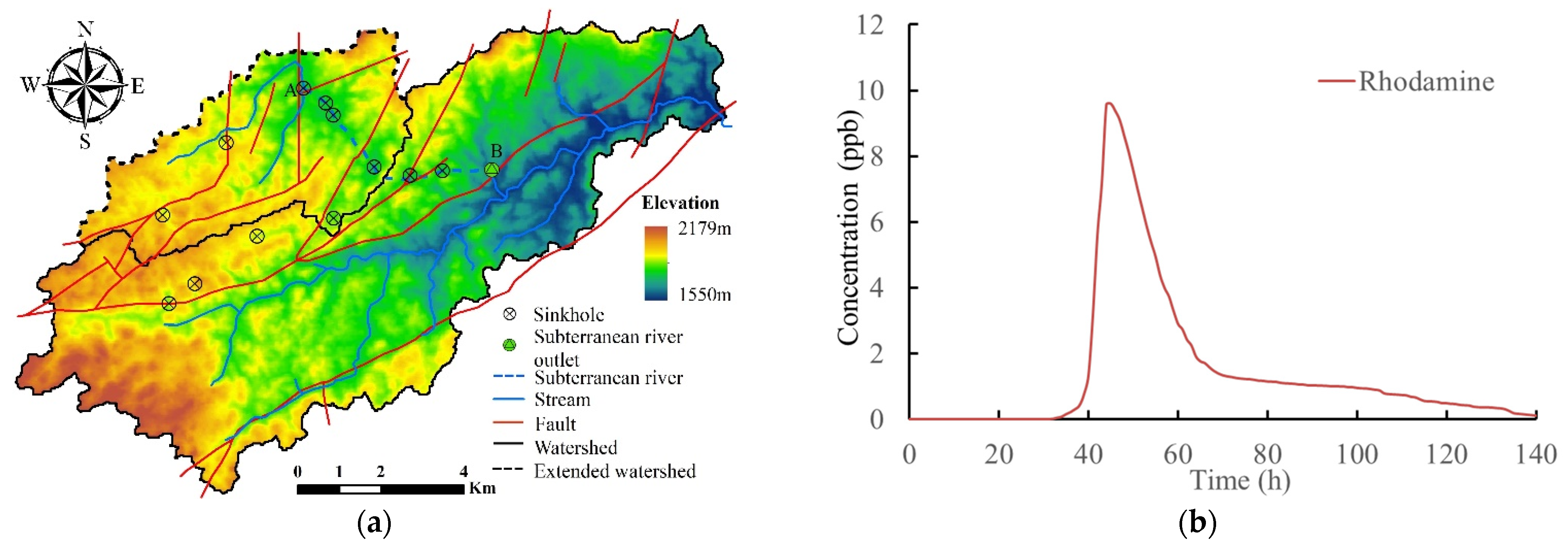
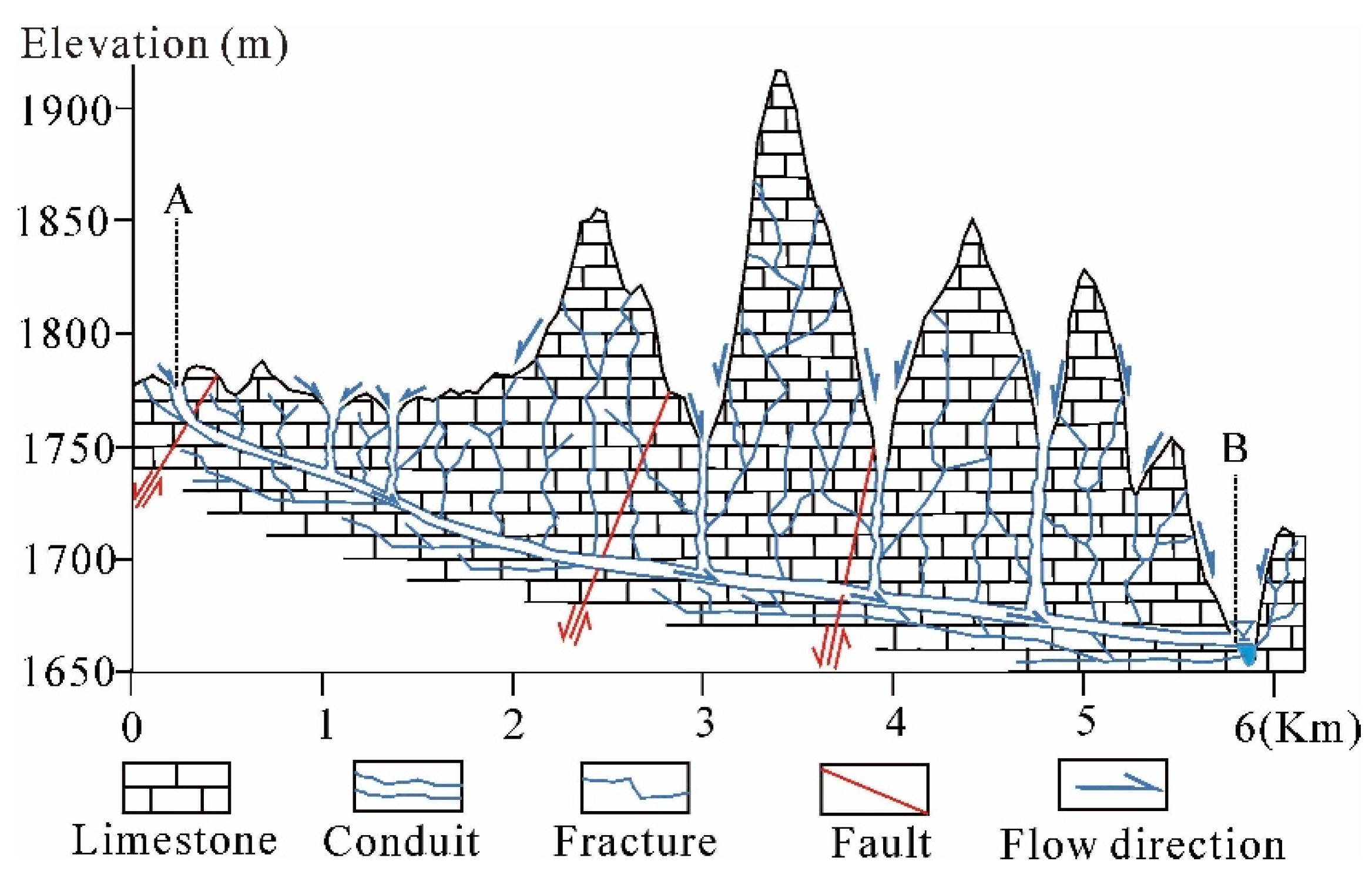
3.3.1. Karst Survey and Tracer Test

Karst survey and artificial tracer test serve as important ways of identifying the flow paths and hydrological characteristics of karst subterranean rivers [39]. In August 2018, a field survey was conducted in the study area before modeling, and the main purpose of this was to determine the spatial distribution of subterranean river inlet, ponors, and sinkholes. Multiple sinkholes are distributed on the ground surface of the catchment area (Figure 4a); point A is the inlet of the subterranean river, and point B is the large outlet of the subterranean river in the watershed. The straight-line distance between points A and B is 5.1 km. To determine whether point A is connected to point B, an artificial tracer test was carried out from 15 August to 25 August 2018, by injecting 4 kg of rhodamine at point A and detecting it at point B using GGUN-FL30 fluorometers. The results of the tracer test were quantitatively assessed using the software, QTRACER2 [40].

3.3.2. DEM Data Modification

DEM data are the major basis for defining the catchment scope of a watershed in the SWAT model. After determining the flow paths of subterranean rivers, the conversion of subterranean rivers into surface rivers by modifying DEM data can improve the integrity of the SWAT model in identifying catchment boundaries based on DEM data. The detailed steps are as follows: (1) Determine the flow paths of subterranean rivers according to the flow direction of subterranean rivers and the spatial distribution characteristics of ponors; (2) Extract the grid data corresponding to the flow paths of subterranean rivers from the original DEM data using ArcGIS; (3) Convert the grid data extracted into point data, and set the attribute values of the point data as elevation values; (4) Modify the elevation values of the point data according to the slope between the inlet and outlet of each subterranean river, and convert the point data modified into grid data; (5) Merge the modified grid data into the original DEM data.

3.4. Model Setup

In this study, the catchment scope of the watershed was identified by loading the DEM data using the ArcSWAT interface. To determine the minimum area threshold of the sub-watersheds, it was necessary to compare the closest degree between the simulated river network and the real river network. In this study, the minimum-area threshold of sub-watersheds was set at 200 ha, and the thresholds of land cover data and soil data used for dividing HRUs were set at 10%. That is, any data on land use and soil below this threshold was ignored in the model. The Natural Breaks (Jenks) classification method in ArcGIS was used to classify the watershed terrain slope into three threshold ranges: 0°–8.6°, 8.6°–18.6° and >18.6°, respectively.

The period from 1990 to 1992 was taken as the warm-up period, and the time increment for result output was set at one day. The observed daily runoff data during 1993–1998 were used for calibration. The annual precipitation in the calibration period (1993–1998) was normal. Considering the large difference in annual precipitation from 1999 to 2006, the validation period was divided into two parts. The first validation period was from 1999 to 2002 and was named validation A. This period included three types: normal, dry, and wet year. The second validation period was from 2003 to 2006 and was named validation B. This period only included two types: normal and dry year.

3.5. Model Calibration, Validation, and Performance Evaluation

The program Sequential Uncertainty Fitting Ver. 2 (SUFI-2) of SWAT-CUP was selected for the calibration and validation of the modified and original SWAT models. Meanwhile, the global sensitivity analysis was used to rank the parameter sensitivity of the two models. In this sensitivity analysis method, the smaller the p-value and the larger the absolute value of t-stat, the more sensitive the parameter is [41].

Uncertainty in SUFI2 parameters conveyed as ranges (uniform distributions), accounts for total sources of uncertainties such as uncertainty in driving variables (e.g., rainfall), observed data, conceptual models, and parameters [42]. Propagation of the parameter uncertainties results in uncertainties in the SWAT model output variables, which are manifested as the 95% probability distributions (i.e., 95PPU). P-factor and R-factor are indices used by SUFI-2 to evaluate the model uncertainty performance [43]. The P-factor is the proportion of observed data enveloped by the simulation results, the 95PPU, while the R-factor is the breadth of the 95PPU band. If P-factor is greater than 70% and R-factor is less than 1, the model results are considered acceptable [44].

The coefficient of determination (R²), Nash–Sutcliffe efficiency (NSE) coefficient, and percent bias (PBIAS) were used to evaluate the performance and efficiency of the SWAT model. The coefficient of determination (R²) can be used to characterize the degree of correlation between simulated values and measured values [45]. Its values vary in the range of 0–1. The closer to 1 the value of R², the higher the degree of correlation between simulated values and measured values. NSE is a standardized statistic, determining the deviation of the residual variance from the variance of measured data. Its values vary in the range of −∞–1. The closer to 1 the NSE value, the closer the measured value is to the simulation result [46]. PBIAS can be used to characterize the average trend that the simulated data are greater or less than the observed data, with positive and negative values indicating underestimation and overestimation deviation, respectively [47]. R² ≥ 0.5, NSE ≥ 0.5, and −25% < PBIAS < 25% in the calibration period indicate that the simulation efficiency can meet modeling requirements [47,48]:

$${\mathrm{R}}^2=\frac{{\left[{\sum }_{i=1}^n\left(O_i-\overline{O}\right)\left(S_i-\overline{S}\right)\right]}^2}{{\sum }_{i=1}^n{\left(O_i-\overline{O}\right)}^2{\sum }_{i=1}^n{\left(S_i-\overline{S}\right)}^2}$$

(7)

$$\mathrm{NSE}=1-\frac{{\sum }_{i=1}^n{\left(O_i-S_i\right)}^2}{{\sum }_{i=1}^n{\left(O_i-\overline{O}\right)}^2}$$

(8)

$$\mathrm{PBIAS}=\frac{{\sum }_{i=1}^n\left(O_i-S_i\right)\times 100}{{\sum }_{i=1}^n{O}_i}$$

(9)

where O_i is the observed flow (m³/s), S_i is the simulated flow (m³/s), $\overline{O}$ is the average observed flow(m³/s), $\overline{S}$ is the average simulated flow (m³/s), and n is the total number of observed flow.

4. Results

4.1. Identification of Flow Path of Karst Subterranean River

The duration curve of rhodamine concentration at the outlet of the subterranean river is the single-peak type (Figure 4b), indicating that the karst conduit is relatively single, and there is no branch and pool development. According to the evaluation results of the tracer test by the QTRACER2 software, the overall percent recovery of tracer at point B (Figure 4a) is 90.51% (

Table 3. Tracer test results of subterranean rivers calculated using QTRACER2.

Physical Parameters of Subterranean Rivers	Value
Average tracer velocity (m/h)	119.67
Time to peak tracer concentration (h)	45.7
Maximum tracer velocity (m/h)	210.51
Cross-sectional area of conduits (m2)	13.765
Surface area of subterranean rivers (m2)	3.68 × 107
Diameter of conduits (m)	4.19
Péclet number	7.19
Reynolds number	1.22 × 105
Percent recovery of tracer injected	90.51%

), indicating that point B is the concentrated discharge point of the subterranean river. The calculated values of average and maximum migration velocities of tracer from point A to point B are 119.67 m/h and 210.51 m/h, respectively. The surface area of the subterranean river is estimated to be 3.68 × 10⁷ m². The estimated diameter and cross-sectional area of karst conduits are 4.19 m and 13.765 m², respectively. Meanwhile, the estimations of Reynolds number and Peclet number are 1.22 × 10⁵ and 7.19, respectively, indicating that the flow characteristics of the subterranean river are similar to the characteristics of the surface river.

Sinkholes are a karst form of ground collapse caused by the constant development of underground karst caves [49,50]. The bottom of sinkholes are generally connected with the conduits of subterranean rivers. Therefore, it can be determined that the connecting line of the sinkholes between points A and B is the water flow path of the subterranean river (dotted blue line in Figure 4a), covering a distance of 6.2 km. Based on DEM data, stratum conditions and the distribution of sinkholes, the cross-section schematic diagram of the subterranean river was obtained (Figure 5). Depressions on the ground surface are connected to the subterranean river conduit through sinkholes, and thus the surface runoff in the depressions can flow into the subterranean river conduit through sinkholes. Therefore, each depression that is connected to a subterranean river through a sinkhole can be considered as a sub-watershed of the subterranean river.

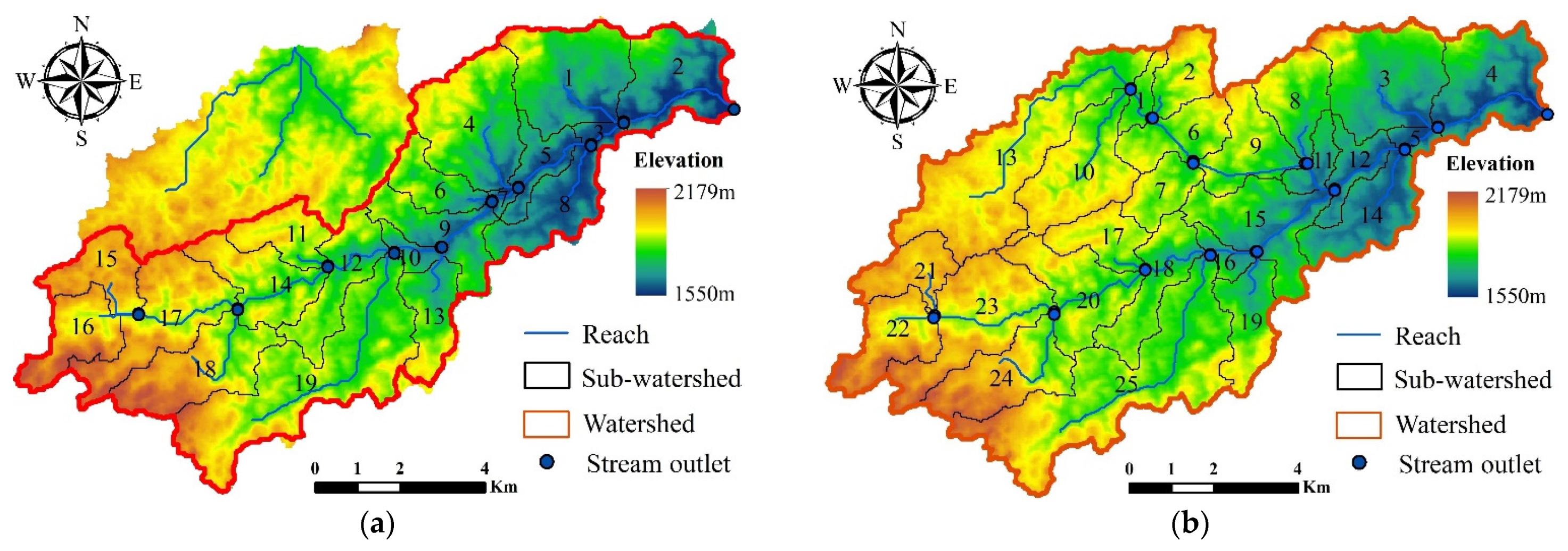
4.2. Results of Sub-Watershed Division Based on Modified DEM Data

The sub-watersheds of the Daotian River watershed were identified using the ArcSWAT interface based on the minimum area threshold of sub-watersheds.

The identification results of sub-watersheds using original DEM data are shown in Figure 6a. When loading the original DEM by ArcSWAT to identify the catchment area of watersheds, the areas at point A and point B were considered to be two independent basins under the influence of karst topography. The identified catchment area only accounted for 76.77% of the total watershed area (the area defined by the red line). A total of 19 sub-watersheds were identified, among which the No.2 sub-watershed was the outlet of the whole watershed. Figure 5 shows the reason why the areas beyond the topographic drainage divides are not identified as the catchment area of the watershed, and there is no continuous channel between points A and B.

In order to identify the catchment area of point A as the catchment area of the watershed, a river channel was pre-defined between point A and point B. The original DEM of the study area was modified according to the method mentioned in Section 3.3.2 to convert the subterranean river into a surface river. Based on the modified DEM, a total of 25 sub-watersheds were determined by ArcSWAT, among which the No.4 sub-watershed was the outlet of the watershed instead (Figure 6b). In this way, the areas beyond the topographic drainage divides were identified as six sub-watersheds (No. 1, 2, 6, 7, 10, 13) of the watershed.

Based on the division of sub-watersheds, the study area was further divided into 389 HRUs according to the slope, land cover, and soil data of the study area, as well as given thresholds.

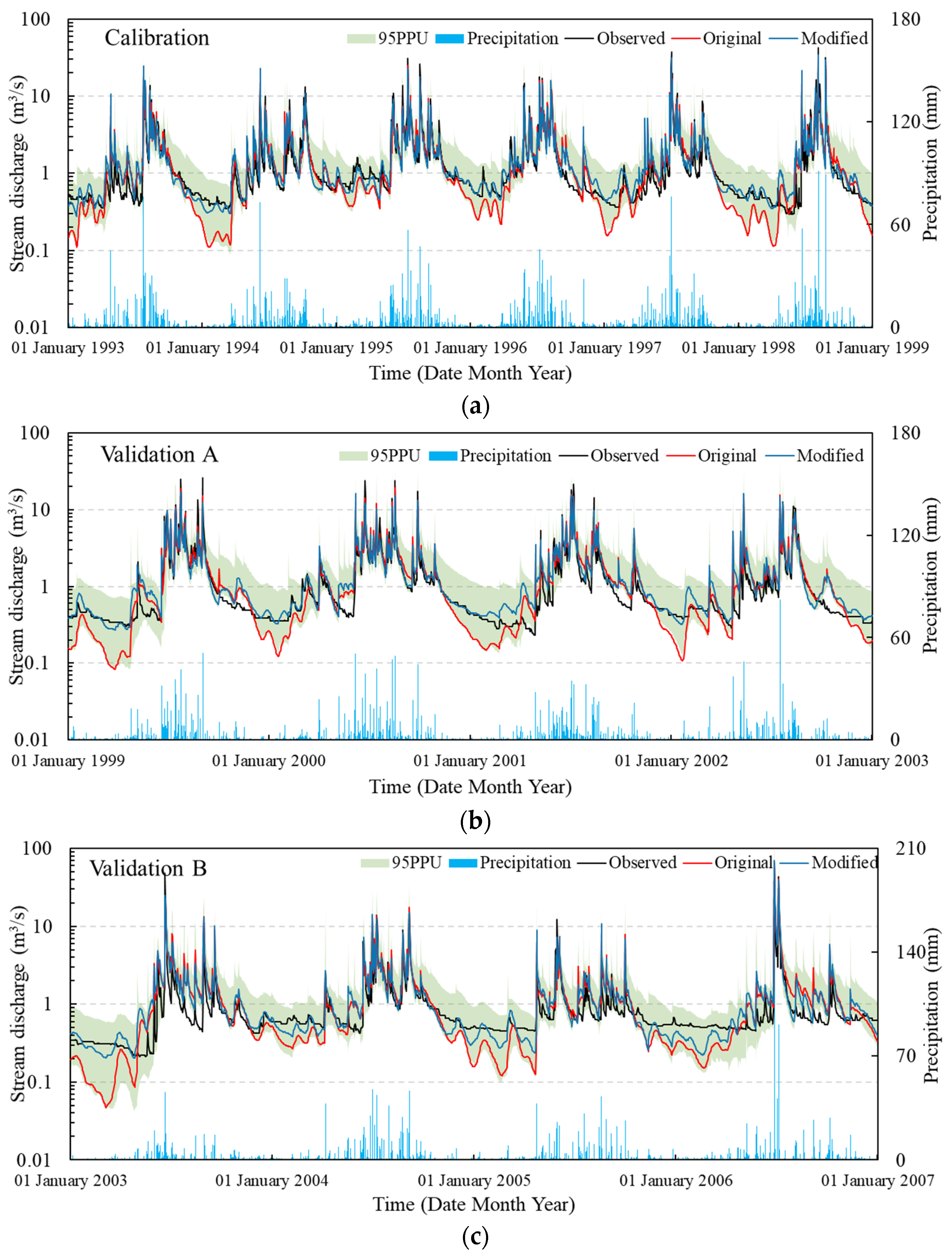
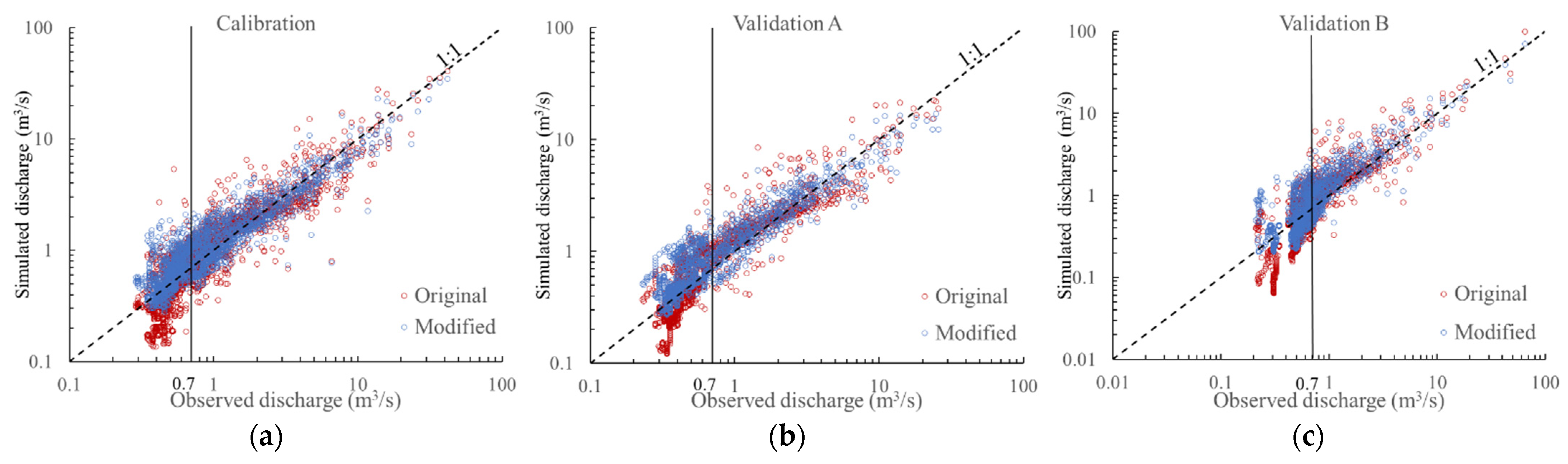
4.3. Calibration, Validation, and Performance Evaluation

Based on the literature [17], 10 and 17 parameters (

Table 4. Sensitivity ranking and values of the parameters for calibration of the modified and the original SWAT model for the Daotian River catchment.

Parameter	Range	Modified SWAT Model				Original SWAT Model
		Rank	t-Stat	p-Value	Fitted Value	Rank	t-Stat	p-Value	Fitted Value
R_CN2	[0, 0.5]	1	−24.34	0.00	0.21	1	−11.57	0	0.19
V_PND_FR	[0, 1]	2	−17.35	0.00	0.09
V_ESCO	[0.75, 1]	3	−3.57	0.00	0.85	10	−0.4	0.69	0.85
V_GW_REVAP	[0, 0.2]	4	2.96	0.00	0.01	9	−0.61	0.54	0.005
R_SOL_BD (1 *)	[0, 0.5]	5	2.74	0.01	0.33	3	4.78	0	0.32
V_αlow	[0, 1]	6	−2.03	0.04	0.00
V_ALPHA_BNK	[0.2, 0.6]	7	1.72	0.09	0.45	8	0.8	0.42	0.42
V_CH_N2	[0.01, 0.04]	8	1.23	0.22	0.02	2	5.52	0	0.019
V_GW_DELAY	[10, 200]	9	−1.13	0.26	107.70	6	0.99	0.32	100
R_SOL_K (1 *)	[0, 0.5]	10	−1.13	0.26	0.42	4	3.41	0	0.41
V_β1	[0, 0.5]	11	0.86	0.39	0.11
V_αmid	[0, 1]	12	0.79	0.43	0.05
V_αup	[0, 1]	13	−0.65	0.51	0.01
V_CH_K2	[85, 140]	14	0.47	0.64	136.30	5	1.26	0.21	105
V_β2	[0.5, 1]	15	−0.39	0.70	0.91
V_β3	[0.5, 1]	16	−0.23	0.82	0.45
V_Kd	[0, 10]	17	−0.12	0.91	1.56
V_ALPHA_BF	[0, 1]					7	0.96	0.34	0.018

1 *: Topsoil. The parameter-based model calibration in this study is conducted based on ‘V_’ and ‘R_’, which denote a replacement and change relative to the initial parameter value, respectively.

) that had significant effects on the runoff simulation of small watersheds were selected for the model calibration of the original and modified SWAT models, respectively. Then, the parameter sensitivity analysis and calibration of the two models were conducted. Since new parameters (Table 1) were added into the groundwater module in the modified SWAT model, more parameters were selected for the modified SWAT than for the original SWAT model.

The algorithm of the groundwater module in the modified SWAT model is different from that of the original SWAT model, so the parameters of the two models must be calibrated separately. After 1000 iterations of SUFI-2 algorithm in SWAT-CUP, the fitted value and sensitivity ranking of parameters used in the original and the modified SWAT model (Table 4) and daily flow simulation results (Figure 7) were determined. The parameters that have significant effects on runoff simulation (p-value < 0.05) include CN2, CH_N2, SOL_BD (1), and SOL_K (1) in the original SWAT model. In contrast, they include CN2, PND_FR, ESCO, GW_REVAP, SOL_BD (1), and α_low in the modified SWAT model.

The runoff curve number (CN2) and the moist bulk density of topsoil (SOL_BD (1)) are identified as the common sensitive parameters of the original and modified SWAT models. In addition, CN2 is the most sensitive parameter of both models, which is consistent with other studies. Boughton found that the ±10% change in the CN value could lead to a −45–55% fluctuation in the runoff [51].

However, there are still significant differences in parameter sensitivity between the original and modified SWAT models. For example, the parameters that affected evapotranspiration (ESCO, GW_REVAP) are sensitive parameters only in the modified SWAT model. On the contrary, the Manning’s roughness coefficient of river channels (CH_N2) and the saturated hydraulic conductivity of topsoil (SOL_K (1)) are sensitive parameters only in the original SWAT model. In addition, the parameter ALPHA_BF that controls groundwater recession is not a sensitive parameter in the original SWAT mode. However, some parameters (PND_FR, α_low) related to groundwater recharge and recession become sensitive parameters in the modified SWAT model. Furthermore, PND_FR is the second key sensitive parameter surpassed only by CN2, which is attributable to the fact that PND_FR is the key parameter determining the proportion of surface water converted into groundwater. Therefore, the changes in parameter sensitivity are related to the modifications of algorithms in the SWAT model, and it was reported that the changes in model algorithms lead to the changes in parameter sensitivity [13].

Table 5. Performance summary of original and modified SWAT models in calibration and validation periods.

Simulation Periods	Modified SWAT Model					Original SWAT Model
	P-Factor	R-Factor	R2	NSE	PBIAS	P-Factor	R-Factor	R2	NSE	PBIAS
Calibration (1993–1998)	0.89	0.51	0.88	0.87	2.5%	0.81	0.50	0.84	0.83	3.4%
Validation A (1999–2002)	0.88	0.52	0.84	0.83	−1.9%	0.80	0.51	0.79	0.77	−2.2%
Validation B (2003–2006)	0.86	0.51	0.86	0.85	−15%	0.79	0.50	0.82	0.81	−16%

shows that the P-factor, R-factor, and NSE of both the original and the modified SWAT model are greater than 0.7, less than 1, and greater than 0.75, respectively, in the calibration (1993–1998) (Figure 7a), validation A (1999–2002) (Figure 7b), and validation B (2003–2006) periods (Figure 7c), indicating excellent simulation results. Meanwhile, the absolute values of PBIAS of the two models are less than 25%. Therefore, the simulation results of both the original and the modified SWAT model meet the accuracy requirements.

According to Table 5, the P-factor of the modified SWAT model is greater than that of the original SWAT model in both the calibration period and the validation periods, A and B, indicating that the uncertainty of the modified SWAT model is lower than that of the original SWAT model. In addition, the modified SWAT model surpasses the original SWAT model in terms of R², NSE, and PBIAS. Based on this and the output results (Figure 7a–c), it can be seen that the output results of the modified SWAT model are more accurate than those of the original SWAT model.

According to the conceptual model (Figure 2), the modified SWAT model is equivalent to the original SWAT model in the case that Q_kr is zero (no karst recharge) and both β₁ and β₂ are zero. In this case, the optimal values of the common parameters of the original and modified SWAT models are very close (Table 4). Therefore, the simulated values of the original SWAT model are all close to the bottom of the 95PPU band of the modified SWAT model during low-flow periods.

Figure 8a–c show the difference between the original and modified SWAT model outputs during low-flow periods. No matter the calibration or the two validation periods, when the observed flow is less than 0.7 m³/s, the original SWAT is more likely to underestimate the flow than the modified SWAT.

The code modification of this study is mainly focused on the groundwater module of SWAT. Therefore, it is necessary to compare the performance of original and modified SWAT in baseflow simulation. Baseflow Filter Program (https://swat.tamu.edu/software, accessed on 7 February 2021) can separate the baseflow from streamflow. Figure 9 shows the difference between an original and modified SWAT model in modeling the baseflow from 1993 to 2006. The Nash efficiency coefficient of the modified SWAT model is 0.09 higher than that of the original SWAT model in simulating baseflow. It can be seen from Figure 9, in terms of baseflow simulation, that the original SWAT overestimates the base flow in wet seasons and underestimates the base flow in dry seasons. However, the modified SWAT model has clear advantages in reproducing the base flow.

4.4. Water Balance Components

Table 6. Water balance components in the Daotian River watershed calculated using the original and modified SWAT models.

Hydrologic Component	Original SWAT Model	Modified SWAT Model
Average amount of precipitation in the watershed (mm)	935.7	935.7
Actual evapotranspiration (mm)	514.3 (55.0% amount of precipitation)	512.4 (54.7% amount of precipitation)
Water yield (mm)	417.3 (44.6% amount of precipitation)	419.0 (44.8% amount of precipitation)
Surface runoff (mm)	176.2 (18.8% amount of precipitation)	167.1 (17.9% amount of precipitation)
Lateral flow contribution to stream (mm)	171.6 (18.3% amount of precipitation)	147.9 (15.8%) amount of precipitation
Total groundwater recharge (mm)	73. 9 (7.9% amount of precipitation)	108.5 (11.6% amount of precipitation)
Groundwater evapotranspiration (mm)	4.1 (5.5% groundwater recharge)	4.3 (4.0% groundwater recharge)
Groundwater contribution to stream (mm)	69.5 (94.0% groundwater recharge)	104.0 (93.5% groundwater recharge)

shows the 1993–2006 average annual water balance components in the Daotian River watershed, calculated using the original and modified SWAT models. The water balance results of both models show that the actual evapotranspiration (ET) is the largest water consumption item in the watershed, accounting for 55% and 54.7% of the total amount of precipitation in the two models, respectively. This is consistent with the previous study results of similar areas [21].

There are clear differences in water balance components between the original and modified SWAT models. For example, the actual evapotranspiration, surface runoff, and lateral flow in the original SWAT model are greater than those in the modified SWAT model, while the groundwater recharge and the contribution of groundwater to river channels in the modified SWAT model are greater than those in the original SWAT model. The reason is that the groundwater recharge in the modified SWAT model includes not only infiltration recharge from the soil bottom but also the rapid recharge from karst groundwater in fractures and sinkholes. In this way, it can be ensured that the river channel flow is equivalent to the actual observed data in low flow periods. Since a part of the surface runoff and lateral flow in each HRU in the modified SWAT model will flow into the pond and convert into the rapid groundwater recharge, the surface runoff and lateral flow in the modified SWAT model are less than those in the original SWAT model.

5. Discussion

For small karst watersheds, the correct identification of the catchment boundaries of the watersheds is critical for the balance between the water, solutes, and sediments in the watersheds. Although the discharge characteristics of well-developed karst conduits are similar to those of streams [52,53], the hydraulic conductivity of the conduit network is usually unknown. Therefore, it is reasonable to identify the flow paths of the main conduits of the subterranean river based on field surveys and artificial tracer tests, and then simplify the subterranean river into a surface river by modifying the DEM data in this study (Figure 6b). This not only ensures the identification accuracy of actual catchment boundaries but also improves the adaptability of the SWAT model to karst watersheds where the surface drainage divides are inconsistent with the actual catchment boundaries. This processing is equivalent to the method of predefining a watershed system. For some watersheds with gently varying terrain, the water system in the watersheds cannot be identified using rough DEM data and it is necessary to predefine the water system in the watersheds according to actual situations [54].

The prerequisite for obtaining high-precision hydrological simulation results is to ensure the full definition of the basic model [42]. Compared with previous studies, a field survey and tracer tests were carried out before modeling in this study, thus verifying the accuracy of the basic model. It should be noted that the P-factor is only 0.68 in the case that the model is established using the original DEM data (Figure 6a). In this case, the modeling requirements are not met [44]. In contrast, the P-factor is 0.81 in the validation period (original SWAT model), provided that the model is built using the DEM data that are modified to simplify the subterranean river into a surface river (Figure 6b), indicating that the basic model is credible. It also indicates that the model is more important for correctly identifying the catchment area of karst watersheds for karst hydrological modeling than modifying the SWAT model. Moreover, richer precipitation data are used in this study compared to previous studies. Four rain-gauging stations and one weather station (Figure 1) are distributed at different elevations within 99 km² of catchment area in the study area, which reduces the spatial uncertainty of precipitation in the study area. Therefore, the accuracy (Table 5) of simulation results obtained even using the original SWAT model in this study is higher than that of the results of previous relevant studies that utilized SWAT to simulate the runoff in small karst watersheds [21,35]. This also reveals that the observed precipitation data serve as a major factor affecting the accuracy of the SWAT model [55,56]. The quality of input data (e.g., meteorological data, topographic data, land use data and soil data) is also an important factor affecting the accuracy of hydrological model, and the accuracy of modified SWAT model also decreases in areas with insufficient data.

Although a previous study showed that satisfactory simulation results could also be obtained using the original SWAT model when applied to karst watersheds [21], the simulation results of the study were monthly data. The results of this study showed that the original SWAT model could not output satisfactory daily simulation results during low-flow periods (Figure 8a–c) since it underestimated the water quantity during low-flow periods. However, the runoff during low-flow period greatly influences the evaluation accuracy of water resources and droughts in karst watersheds [20,57]. In low-flow periods, the flow is mainly maintained by the base flow, and groundwater discharge is the key to control the base flow. Affected by multiple karst media, the discharge of a karst aquifer has multi-level attenuation characteristics [58]. The modified SWAT groundwater module in this study better coincides with the actual conditions of the karst water cycle in South China. As a result, the modified SWAT model can effectively increase the groundwater recharge (Table 6) and enhance the simulation accuracy of daily baseflow (Figure 9). Furthermore, within the same parameter ranges, the uncertainty of the modified SWAT model is lower (Table 5) than that of the original SWAT model. The modified SWAT model has advantages in karst areas that lack information or knowledge such as water conductivity and water supply degree. The drainage effect of the three reservoirs can effectively describe the drainage characteristics of a karst aquifer, thus improving the accuracy of water resources evaluation in these areas.

6. Conclusions

In the hydrological modeling of small karst watersheds, it is necessary to validate the catchment boundaries of the watersheds according to the hydrogeological conditions before modeling since the basic model cannot be sufficiently defined if the catchment area of watersheds is identified only according to topographic drainage divides.

In the modeling of watersheds containing karst subterranean rivers using the SWAT model, it is feasible to determine the flow paths of subterranean rivers through karst surveys and artificial tracer tests and to simplify karst subterranean rivers into surface rivers. This modeling approach can improve the adaptability of the SWAT model to karst watersheds where the surface drainage divides are inconsistent with actual catchment boundaries.

The model bearing three linear reservoirs and the groundwater recharge through pond leakage is used in the modified SWAT groundwater module. This can improve the quality of the conceptual model, reduce the uncertainty of the SWAT model, and enhance the simulation accuracy of daily runoff. The modified SWAT has clear advantages over the original SWAT in reproducing the baseflow, and its Nash efficiency coefficient is 0.09 higher than that of the original SWAT in simulating baseflow.

References

1. Ford, D.; Williams, P.D. Karst Hydrogeology and Geomorphology; John Wiley & Sons: Hoboken, NJ, USA, 2007. [Google Scholar]
2. Jimenez-Martinez, J.; Longuevergne, L.; Le Borgne, T.; Davy, P.; Russian, A.; Bour, O. Temporal and spatial scaling of hydraulic response to recharge in fractured aquifers: Insights from a frequency domain analysis. Water Resour. Res. 2013, 49, 3007–3023. [Google Scholar] [CrossRef] [Green Version]
3. Ojha, R.; Ramadas, M.; Govindaraju, R.S. Current and Future Challenges in Groundwater. I: Modeling and Management of Resources. J. Hydrol. Eng. 2015, 20, A4014007. [Google Scholar] [CrossRef]
4. Goldscheider, N.; Drew, D. Methods in Karst Hydrogeology; Taylor & Francis: London, UK, 2007. [Google Scholar]
5. White, W.B. Karst hydrology: Recent developments and open questions. Eng. Geol. 2002, 65, 85–105. [Google Scholar] [CrossRef]
6. Pardo-Iguzquiza, E.; Dowd, P.; Bosch, A.P.; Luque-Espinar, J.A.; Heredia, J.; Duran-Valsero, J.J. A parsimonious distributed model for simulating transient water flow in a high-relief karst aquifer. Hydrogeol. J. 2018, 26, 2617–2627. [Google Scholar] [CrossRef]
7. Dar, F.A.; Perrin, J.; Ahmed, S.; Narayana, A.C. Review: Carbonate aquifers and future perspectives of karst hydrogeology in India. Hydrogeol. J. 2014, 22, 1493–1506. [Google Scholar] [CrossRef]
8. Belcher, W.R.; Bedinger, M.S.; Back, J.T.; Sweetkind, D.S. Interbasin flow in the Great Basin with special reference to the southern Funeral Mountains and the source of Furnace Creek springs, Death Valley, California, U.S. J. Hydrol. 2009, 369, 30–43. [Google Scholar] [CrossRef] [Green Version]
9. Nikolaidis, N.P.; Bouraoui, F.; Bidoglio, G. Hydrologic and geochemical modeling of a karstic Mediterranean watershed. J. Hydrol. 2013, 477, 129–138. [Google Scholar] [CrossRef]
10. Baffaut, C.; Benson, V.W. Modeling Flow and Pollutant Transport in a Karst Watershed with SWAT. Trans. ASABE 2009, 52, 469–479. [Google Scholar] [CrossRef]
11. Afinowicz, J.D.; Munster, C.L.; Wilcox, B.P. Modeling effects of brush management on the rangeland water budget: Edwards plateau, Texas. J. Am. Water Resour. Assoc. 2005, 41, 181–193. [Google Scholar] [CrossRef]
12. Arnold, J.G.; Srinivasan, R.; Muttiah, R.S.; Williams, J.R. Large area hydrologic modeling and assessment part I: Model development. J. Am. Water Resour. Assoc. 1998, 34, 73–89. [Google Scholar] [CrossRef]
13. Pang, S.; Wang, X.; Melching, C.S.; Feger, K.-H. Development and testing of a modified SWAT model based on slope condition and precipitation intensity. J. Hydrol. 2020, 588, 125098. [Google Scholar] [CrossRef]
14. Marahatta, S.; Devkota, L.P.; Aryal, D. Application of SWAT in Hydrological Simulation of Complex Mountainous River Basin (Part I: Model Development). Water 2021, 13, 1546. [Google Scholar] [CrossRef]
15. Asl-Rousta, B.; Mousavi, S.J.; Ehtiat, M.; Ahmadi, M. SWAT-Based Hydrological Modelling Using Model Selection Criteria. Water Resour. Manag. 2018, 32, 2181–2197. [Google Scholar] [CrossRef]
16. Chen, M.; Cui, Y.; Gassman, P.; Srinivasan, R. Effect of Watershed Delineation and Climate Datasets Density on Runoff Predictions for the Upper Mississippi River Basin Using SWAT within HAWQS. Water 2021, 13, 422. [Google Scholar] [CrossRef]
17. Marin, M.; Clinciu, I.; Tudose, N.C.; Ungurean, C.; Adorjani, A.; Mihalache, A.L.; Davidescu, A.A.; Davidescu, S.O.; Dinca, L.; Cacovean, H. Assessing the vulnerability of water resources in the context of climate changes in a small forested watershed using SWAT: A review. Environ. Res. 2020, 184, 109330. [Google Scholar] [CrossRef] [PubMed]
18. Amatya, D.M.; Edwards, A.E. Applying the SWAT hydrologic model on a watershed containing forested karst. Beneath Forest 2009, 1, 12–13. [Google Scholar]
19. Amin, M.G.M.; Veith, T.L.; Collick, A.S.; Karsten, H.D.; Buda, A.R. Simulating hydrological and nonpoint source pollution processes in a karst watershed: A variable source area hydrology model evaluation. Agric. Water Manag. 2017, 180, 212–223. [Google Scholar] [CrossRef] [Green Version]
20. Reza Eini, M.; Javadi, S.; Delavar, M.; Gassman, P.W.; Jarihani, B. Development of alternative SWAT-based models for simulating water budget components and streamflow for a karstic-influenced watershed. Catena 2020, 195, 104801. [Google Scholar] [CrossRef]
21. Jakada, H.; Chen, Z. An approach to runoff modelling in small karst watersheds using the SWAT model. Arab. J. Geosci. 2020, 13, 318. [Google Scholar] [CrossRef]
22. Neitsch, S.L.; Arnold, J.G.; Kiniry, J.R.; Williams, J.R. Soil and Water Assessment Tool Theoretical Documentation Version 2009; Texas Water Resources Institute: College Station, TX, USA, 2011; pp. 169–173. [Google Scholar]
23. Tobin, B.W.; Schwartz, B.F. Quantifying Concentrated and Diffuse Recharge in Two Marble Karst Aquifers: Big Spring and Tufa Spring, Sequoia and Kings Canyon National Parks, California, USA. J. Cave Karst Stud. 2012, 74, 186–196. [Google Scholar] [CrossRef]
24. Jukic, D.; Denic-Jukic, V. Nonlinear kernel functions for karst aquifers. J. Hydrol. 2006, 328, 360–374. [Google Scholar] [CrossRef]
25. Eris, E.; Wittenberg, H. Estimation of baseflow and water transfer in karst catchments in Mediterranean Turkey by nonlinear recession analysis. J. Hydrol. 2015, 530, 500–507. [Google Scholar] [CrossRef]
26. Wang, Y.; Brubaker, K. Implementing a nonlinear groundwater module in the soil and water assessment tool (SWAT). Hydrol. Process. 2014, 28, 3388–3403. [Google Scholar] [CrossRef]
27. Vale, M.; Holman, I.P. Understanding the hydrological functioning of a shallow lake system within a coastal karstic aquifer in Wales, UK. J. Hydrol. 2009, 376, 285–294. [Google Scholar] [CrossRef] [Green Version]
28. Jiang, R.; Li, Y.; Wang, Q.; Kuramochi, K.; Woli, K.P. Modeling the Water Balance Processes for Understanding the Components of River Discharge in a Non-conservative Watershed. Trans. ASABE 2011, 54, 2171–2180. [Google Scholar] [CrossRef]
29. Gamvroudis, C.; Nikolaidis, N.P.; Tzoraki, O.; Papadoulakis, V.; Karalemas, N. Water and sediment transport modeling of a large temporary river basin in Greece. Sci. Total Environ. 2015, 508, 354–365. [Google Scholar] [CrossRef] [PubMed]
30. Malagò, A.; Efstathiou, D.; Bouraoui, F.; Nikolaidis, N.P.; Franchini, M.; Bidoglio, G.; Kritsotakis, M. Regional scale hydrologic modeling of a karst-dominant geomorphology: The case study of the Island of Crete. J. Hydrol. 2016, 540, 64–81. [Google Scholar] [CrossRef]
31. Yactayo, G.A. Modification of the SWAT Model to Simulate Hydrologic Processes in a Karst-Influenced Watershed. Master’s Thesis, Virginia Tech, Blacksburg, VA, USA, 2009. [Google Scholar]
32. Palanisamy, B.; Workman, S.R. Hydrologic Modeling of Flow through Sinkholes Located in Streambeds of Cane Run Stream, Kentucky. J. Hydrol. Eng. 2015, 20, 04014066. [Google Scholar] [CrossRef]
33. Nerantzaki, S.D.; Giannakis, G.V.; Efstathiou, D.; Nikolaidis, N.P.; Sibetheros, I.A.; Karatzas, G.P.; Zacharias, I. Modeling suspended sediment transport and assessing the impacts of climate change in a karstic Mediterranean watershed. Sci. Total Environ. 2015, 538, 288–297. [Google Scholar] [CrossRef]
34. Nerantzaki, S.D.; Nikolaidis, N.P. The response of three Mediterranean karst springs to drought and the impact of climate change. J. Hydrol. 2020, 591, 125296. [Google Scholar] [CrossRef]
35. Wang, Y.; Shao, J.; Su, C.; Cui, Y.; Zhang, Q. The Application of Improved SWAT Model to Hydrological Cycle Study in Karst Area of South China. Sustainability 2019, 11, 5024. [Google Scholar] [CrossRef] [Green Version]
36. Nguyen, V.T.; Dietrich, J.; Uniyal, B. Modeling interbasin groundwater flow in karst areas: Model development, application, and calibration strategy. Environ. Model. Softw. 2020, 124, 104606. [Google Scholar] [CrossRef]
37. Staudinger, M.; Stoelzle, M.; Cochand, F.; Seibert, J.; Weiler, M.; Hunkeler, D. Your work is my boundary condition! Challenges and approaches for a closer collaboration between hydrologists and hydrogeologists. J. Hydrol. 2019, 571, 235–243. [Google Scholar] [CrossRef]
38. Jin, X.; He, C.; Zhang, L.; Zhang, B. A Modified Groundwater Module in SWAT for Improved Streamflow Simulation in a Large, Arid Endorheic River Watershed in Northwest China. Chin. Geogr. Sci. 2018, 28, 47–60. [Google Scholar] [CrossRef] [Green Version]
39. Goldscheider, N.; Meiman, J.; Pronk, M.; Smart, C. Tracer tests in karst hydrogeology and speleology. Int. J. Speleol. 2008, 37, 27–40. [Google Scholar] [CrossRef] [Green Version]
40. U.S. EPA. The Qtracer2 Program for Tracer-Breakthrough Curve Analysis for Tracer Tests in Karstic Aquifers and Other Hydrologic Systems; U.S. Environmental Protection Agency, Office of Research and Development, National Center for Environmental Assessment, Washington Office: Washington, DC, USA, 2002; EPA/600/R-02/001.
41. Abbaspour, K.C. SWAT-CUP 2012: SWAT Calibration and Uncertainty Programs—A User Manual; Swiss Federal Institute of Aquatic Science and Technology: Dubendorf, Switzerland, 2015; pp. 1–100. [Google Scholar]
42. Abbaspour, K.; Vaghefi, S.; Srinivasan, R. A Guideline for Successful Calibration and Uncertainty Analysis for Soil and Water Assessment: A Review of Papers from the 2016 International SWAT Conference. Water 2017, 10, 6. [Google Scholar] [CrossRef] [Green Version]
43. Abbaspour, K.C.; Rouholahnejad, E.; Vaghefi, S.; Srinivasan, R.; Yang, H.; Kløved, B. A continental-scale hydrology and water quality model for Europe: Calibration and uncertainty of a high-resolution large-scale SWAT model. J. Hydrol. 2015, 524, 733–752. [Google Scholar] [CrossRef] [Green Version]
44. Rostamian, R.; Jaleh, A.; Afyuni, M.J.; Mousavi, S.F.; Heidarpour, M.; Jalalian, A.; Abbaspour, K.C. Application of a SWAT model for estimating runoff and sediment in two mountainous basins in central Iran. Hydrol. Sci. J. 2008, 53, 977–988. [Google Scholar] [CrossRef]
45. Nagelkerke, N. A note on a general definition of the coefficient of determination. Biometrika 1991, 78, 691–692. [Google Scholar] [CrossRef]
46. Nash, J.E.; Sutcliffe, J.V. River flow forecasting through conceptual models part I—A discussion of principles—ScienceDirect. J. Hydrol. 1970, 10, 282–290. [Google Scholar] [CrossRef]
47. Moriasi, D.N.; Arnold, J.G.; Liew, M.; Bingner, R.L.; Harmel, R.D.; Veith, T.L. Model Evaluation Guidelines for Systematic Quantification of Accuracy in Watershed Simulations. Trans. ASABE 2007, 50, 885–900. [Google Scholar] [CrossRef]
48. Thavhana, M.P.; Savage, M.J.; Moeletsi, M.E. SWAT model uncertainty analysis, calibration and validation for runoff simulation in the Luvuvhu River catchment, South Africa. Phys. Chem. Earth Parts A/B/C 2018, 105, 115–124. [Google Scholar] [CrossRef]
49. Zhu, X.; Chen, W. Tiankengs in the karst of China. Speleogenesis Evol. Karst Aquifers 2006, 4, 1–18. [Google Scholar]
50. Salvati, R.; Sasowsky, I.D. Development of collapse sinkholes in areas of groundwater discharge. J. Hydrol. 2002, 264, 1–11. [Google Scholar] [CrossRef]
51. Boughton, W.C. A review of the USDA SCS curve number method. Soil Res. 1989, 27, 511–523. [Google Scholar] [CrossRef]
52. Herman, E.K.; Toran, L.; White, W.B. Clastic sediment transport and storage in fluviokarst aquifers: An essential component of karst hydrogeology. Carbonates Evaporites 2012, 27, 211–241. [Google Scholar] [CrossRef]
53. Herman, E.K.; Toran, L.; White, W.B. Threshold events in spring discharge: Evidence from sediment and continuous water level measurement. J. Hydrol. 2008, 351, 98–106. [Google Scholar] [CrossRef]
54. Rahman, M.M.; Thompson, J.R.; Flower, R.J. An enhanced SWAT wetland module to quantify hydraulic interactions between riparian depressional wetlands, rivers and aquifers. Environ. Model. Softw. 2016, 84, 263–289. [Google Scholar] [CrossRef] [Green Version]
55. Yen, H.; Wang, R.; Feng, Q.; Young, C.-C.; Chen, S.-T.; Tseng, W.-H.; Wolfe, J.E.; White, M.J.; Arnold, J.G. Input uncertainty on watershed modeling: Evaluation of precipitation and air temperature data by latent variables using SWAT. Ecol. Eng. 2018, 122, 16–26. [Google Scholar] [CrossRef]
56. Tuo, Y.; Duan, Z.; Disse, M.; Chiogna, G. Evaluation of precipitation input for SWAT modeling in Alpine catchment: A case study in the Adige river basin (Italy). Sci. Total Environ. 2016, 573, 66–82. [Google Scholar] [CrossRef] [PubMed] [Green Version]
57. Fiorillo, F. Spring hydrographs as indicators of droughts in a karst environment. J. Hydrol. 2009, 373, 290–301. [Google Scholar] [CrossRef]
58. Fiorillo, F. Tank-reservoir drainage as a simulation of the recession limb of karst spring hydrographs. Hydrogeol. J. 2011, 19, 1009–1019. [Google Scholar] [CrossRef]
Figure 1. (a) DEM of the Daotian River watershed, (b) Geological map of the Daotian River watershed (extracted from the comprehensive hydrogeological map of Bijie area, China).
Water 13 03552 g001
Figure 2. Conceptual model of the three improved reservoirs for recharge, transformation, and discharge of karst aquifers.
Water 13 03552 g002
Figure 3. (a) Grid data on land use types; (b) Grid data on soil types.
Water 13 03552 g003
Figure 4. (a) Flow path of the subterranean river; (b) Duration curve of the rhodamine concentration recovered at the outlet of the subterranean river.
Water 13 03552 g004
Figure 5. Cross-section schematic diagram of the subterranean river flow path.
Water 13 03552 g005
Figure 6. (a) Watershed and sub-watersheds identified based on original DEM data; (b) Watershed and sub-watersheds identified based on modified DEM data.
Water 13 03552 g006
Figure 7. Simulated daily flow during the calibration period (a) and validation periods A (b) and B (c) obtained using the original and modified SWAT models. The green band denoted the 95PPU of the modified SWAT model.
Water 13 03552 g007
Figure 8. The relationship of observed and two simulated discharges for the calibration period (a) and validation periods A (b) and B (c).
Water 13 03552 g008
Figure 9. Daily baseflow of the original and modified SWAT models during 1993 to 2006.
Water 13 03552 g009