Glacial Lake Evolution (1962–2018) and Outburst Susceptibility of Gurudongmar Lake Complex in the Tista Basin, Sikkim Himalaya (India)

Abstract

The Sikkim Himalayan glaciers and glacial lakes are affected by climate change like other parts of the Himalayas. As a result of this climate variability in the Sikkim Himalaya, a detailed study of the Gurudongmar lake complex (GLC) evolution and outburst susceptibility assessment is required. Glacial lake volume estimation and lake outburst susceptibility assessment were carried out to reveal different characteristics for all four lakes (GL-1, GL-2, GL-3, and GL-4) from the lake complex. Each of these lakes has a moderate to very high potential to outburst. As the dam of GL-1 provides no retention capacity, there is a very high potential of a combined effect with the sudden failure of the moraine-dams of GL-2 or GL-3 located upstream. Temporal analysis of GLC using optical remote sensing data and in-field investigations revealed a rapidly increasing total lake area by ~74 ± 3%, with an expansion rate of +0.03 ± 0.002 km² a⁻¹ between 1962 and 2018 due to climate change and ongoing glacier retreat. The overall lake area expansion rates are dependent on climate-driven factors, and constantly increasing average air temperature is responsible for the enlargement of the lake areas. Simultaneously, changes in GLC expansion velocity are driven by changes in the total amount of precipitation. The deficit in precipitation probably triggered the initial higher rate from 1962 to 1988 during the winter and spring seasons. The post-1990s positive anomaly in precipitation might have reduced the rate of the glacial lake area expansion considerably.

1. Introduction

Glaciers’ response to climate change has been clearly observed throughout the world [1]. Rising temperature has an intertwined relationship with glacier recession and glacial lake evolution in the high mountain areas [2,3]. Glacial lake outburst floods (GLOFs) are common in all areas where glacier retreat is reported. The glacier retreat can be very fast, and many newly incipient glacial lakes could be very prone to outburst [4]. A rapid outburst of glacial lakes can cause a catastrophic flood in the downstream region with great erosive power and debris transport capacity in a short period of time [5,6,7,8,9]. Usually, this is caused by dam breaching or overtopping with a large variety of different triggers, according to local lake position, surrounding landscape, and other natural conditions. Rapid glacial meltwater, extreme rainfall, shock waves produced by mass movements into the lake (i.e., rockfalls, landslide, avalanches, etc.), flood waves from the lake located upstream, ice calving, earthquake, piping, and also “long time triggers”, such as dead-ice melting, hydrostatic pressure, or erosion of a dam, can cause failure or overflow of a dam [10,11]. Sometimes failures also occur due to undercutting slopes by glacio-fluvial erosion and monsoon-induced heavy rainfall leading to saturation and erosion of frontal moraine slopes or loose rock structures hanging over the lakes, together leading to cataclysmic GLOF events [12,13].

One of the most vulnerable areas of very fast deglaciation is Eastern Himalaya [14,15,16], where many historical GLOFs have been reported [17]. It is known that the magnitude of glacier downwasting in Sikkim is relatively faster than for other regions (i.e., Western, Central, and the Karakoram) of the entire Himalaya [18,19,20,21]. The continuous growth of numerous glacial lakes has also been reported on the north face of the Kangchengyao massif of Sikkim Himalaya between 1988 and 2014 by Debnath et al. [22]. An impression of moraine breach in the past signified the occurrence of a GLOF event at Sebu Tso near the base of the Changme Khangpu glacier [23]. Besides these, only a few other studies, on hydrodynamic moraine dam breach modelling and hazard assessment [24], and in–situ bathymetric study [25] of South Lhonak Tso in Sikkim Himalaya, have been reported. Previously, Ives et al. [26] and Worni et al. [27] have reported that the Gurudongmar lakes are considered one of the potentially dangerous lake complexes in the Tista basin of Sikkim Himalaya, and further recommended this for field investigation.

Accurate glacial lake classification is the principal and essential step for the assessment of lake outburst susceptibility. The primary approach is to divide the glacial lake according to the relative position of the mother glacier, proglacial and supraglacial lakes [28], or according to their hydrologic connection to glacial catchments, glacier-fed and non-glacier-fed lakes [29,30]. Based on the above literatures, proglacial, supraglacial, and glacier-fed lakes are dynamic in response to climate change. In contrast, non-glacier-fed lakes are quite stable in nature. Huggel et al. [31], Carrivick and Tweed [32], Worni et al. [27], Emmer et al. [33] and Wilson et al. [34] have divided glacial lakes in the context of their dam type. Based on dam type, moraine-dammed lakes are susceptible to GLOFs because unconsolidated moraine dams may be unstable to the release of large water volumes in the long term. The definitions and classification approaches are broadly explained in Section 3.2.

There is an ongoing knowledge gap in the research of the Gurudongmar lake complex and its fast response to environmental change. Further, the complexity and unique nature of the Gurudongmar Tso area in Sikkim have drawn attention. To address this research gap, we have undertaken this study to analyse the spatio-temporal change of the Gurudongmar lake complex area between 1962 and 2018, estimate the susceptibility of these lakes to outburst floods, and predict future lake complex evolution within the deglaciated catchment. The entire study is based on the analysis of remote sensing data as well as intensive field investigation. The field inspections and measurements were conducted during the period 2017–2018, usually based on visits twice a year, pre-and post-monsoon.

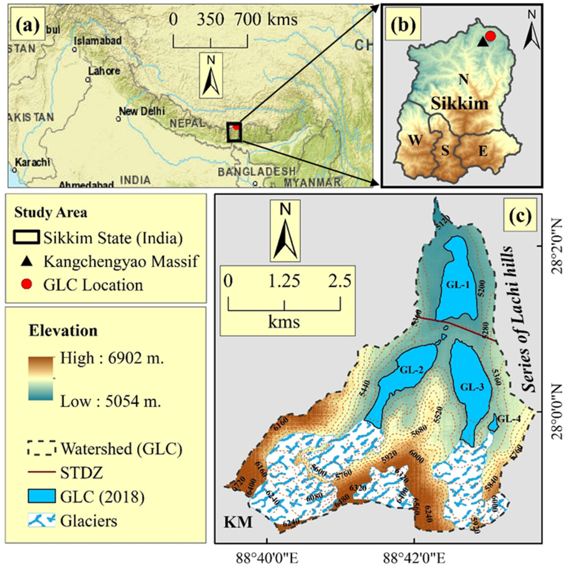
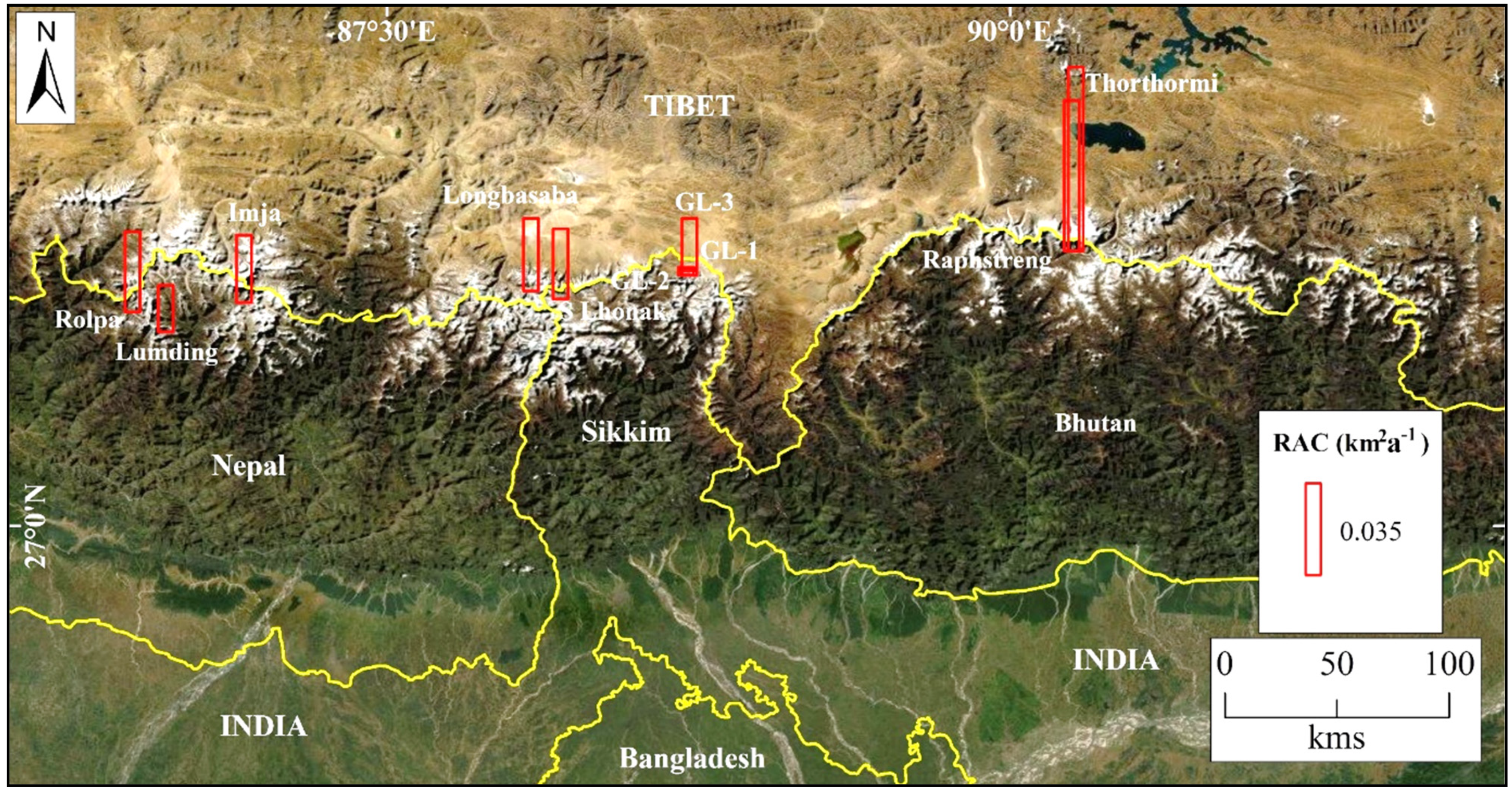
2. Study Area: Gurudongmar Lake Complex

The Gurudongmar lake complex (referred to as GLC hereafter) is a combination of three main glacial lakes (GL-1, GL-2, and GL-3) and one significantly smaller lake, GL-4, which are located on the north face of the Kangchengyao Massif in the Chhombo Chhu watershed of the upper Tista basin in the extreme northeast corner of Sikkim Himalaya (India), a part of Eastern Himalaya (Figure 1). The term “Khangse” means glacier, “Chhu” is a stream, and “Tso or Chho” are lakes, respectively, in the local Tibetan dialect. We will use the local names in the following text. Our area of interest is situated between 27°45′2.23″ N and 28°7′44.48″ N; 88°26′49.89″ E and 88°50′46.28″ E with a varying altitude of 5054–6902 m a.s.l., where the lowest elevation is near the outflow of GL-1 and the highest point on the glaciated mountain crest is above the lake complex. The mean elevations of GL-1 (Gurudongmar Tso), GL-2, GL-3, and GL-4 in the year 2018 were 5154 m, 5220 m, 5262 m, and 5346 m (a.s.l), respectively (see Figure 1c). In the moraine between GL-2 and GL-1, small thermokarst lakes are also located. All the four lakes of the Gurudongmar lake complex are proglacial and glacier-fed but with different dam types. GL-1 is a combined dam-type lake (bedrock and moraine) which is a former proglacial lake because the glacier has already retreated from this area, and frontal moraines and lakes have been created in the upper part of the watershed. Therefore, the overhanging GL-2 and GL-3 are typical frontal moraine-dammed (Mf) lakes. A newly formed proglacial lake, GL-4, originated in the year 2000, is probably dammed by a combination of bedrock and lateral moraine. The proglacial GL-2 and GL-3 are dammed by a frontal moraine formed by recent glaciation (Figure 2). The terminus of Gurudongmar Khangse has abundant steep crevasses, which stretch into the lake GL-3. The GL-2 and GL-3 lakes’ water are fed by the glaciers of Kangchengyao-2 and Gurudongmar Khangse, respectively. Subsequently, water flows into the downstream located GL-1 and finally drains out into the Chhombo Chhu, the uppermost tributary of the Tista River [22]. The glaciers, as mentioned earlier, are also retreating. The accumulation of meltwater in the lakes (GL-2 and GL-3) has significantly increased in volume, leading to growth in the area of these proglacial moraine-dammed lakes (Figure 2). Overall, the entire GLC represents a typical paternoster lake system [35], resembling a series of glacial lakes connected by single or braided streams with a surface or subsurface drainage system.

Geologically, the study area lies in a complex transition zone between the Greater Himalayan Sequence (GHS) in the south and the Tethyan Sedimentary Sequence (TSS) in the north, which is separated by the South Tibetan Detachment Zone (STDZ) [36,37]. This imaginary STDZ passes through the frontal moraine of GL-2 and GL-3, just above the inlet to GL-1 (Figure 1c). GLC is bounded by a series of rounded hillocks (about 300 m from the adjacent plains) called Lachi Hills in the East, and these are formed by an alternative sequence of quartzite and shale with some pebble beds [37]. Rocks of the Everest limestone embody the principal lithology of the catchment area (e.g., limestone, quartzite, sandstone) and crystalline gneissic complex (e.g., quartzite, gneiss, etc.) formations [38]. Moreover, the study site and its surrounding areas have a history of numerous seismic events and hence are seismically active [39,40].

The broader area of the Gurudongmar lake complex indicates signs of structurally predisposed relief with extensive outwash plains that are visible on satellite images without vegetation cover. The highest elevations were under strong glaciations in the past, and various generations of moraines are well pronounced. The north-facing slope of the Kangchengyao massif seems to be more glacially eroded with several lake basins. Nevertheless, this could be a misinterpretation because southern flanks are still more glaciated, and the relief underneath is neither visible nor comparable. Both types of glaciers, valley tongues as well as slope glaciers, are present.

The climate of the investigated (GLC) area is governed by the orographic barrier of the Kangchengyao massif (Figure 1b,c) and an extended part of the Trans-Himalayan region and Tibetan plateau [41]. This region is dominated by cold semi-arid deserted climatic conditions [22]. It shows contrasting climatic and topographic variability within the Sikkim Himalaya [20]. The precipitation occurs in the form of snow, generally influenced by the Indian summer monsoon (ISM) and mid-latitude westerlies (late November to May) [42].

3. Materials and Methods

3.1. Data Sources and Field Surveys

Remotely sensed optical images such as historical declassified Corona KH-4 (1962), Hexagon KH-9 (1975), Landsat 5 TM (1988), Landsat 7 ETM+ (2000), Landsat 5 TM (2010), and Sentinel 2A MSI (2018) have been used to compile the glacial lake inventories (

Table 1. Satellite remote-sensing data used in the current study.

Date of Acquisition	Satellite Sensors	Spatial Resolution (m)	Spectral Bands
24 November 1962	Corona (KH-4)	2.8	Panchromatic
20 December 1975	Hexagon (KH-9)	4	Panchromatic
1 December 1988	Landsat 5 (TM)	30	Visible; mid-infrared
8 November 2000	Landsat 7 (ETM+)	15; 30	Panchromatic; visible; mid-infrared
14 December 2010	Landsat 5 (TM)	30	Visible; mid-infrared
26 November 2018	Sentinel (2A MSI)	10; 20	Visible; shortwave-infrared

Note: KH, keyhole; TM, thematic mapper; ETM+, Enhanced Thematic Mapper Plus; MSI, multi-spectral instrument.

). We acquired all the remote-sensing datasets between November-December (post-monsoon or end of ablation period) to avoid maximum coverage of seasonal snow, cloud, and shadow effects [43]. High-resolution (1.65 to 2.62 m) images on Google Earth (GE) platform have been used to cross-verify the lake outlines of different date datasets. The vertical accuracy of the Shuttle Radar Topography Mission Digital Elevation Model (SRTM DEM) has been found to be better statistically than ASTER and Cartosat-1 DEMs in the study region [22]. Hence, the SRTM DEM (2000) with a spatial resolution of 30 m has been used to extract topographic parameters, such as elevation, slope, and aspects. All the satellite images and SRTM DEM have been obtained from the United States Geological Survey (USGS) portal (http://earthexplorer.usgs.gov/ accessed on 10 January 2021).

Necessary information on the surrounding geomorphology of the glacial lakes and the potential for lake impacts were identified in the field surveys during 2017–2018 and further verified in GE platform. The glacial lakes and associated morphology have been verified using a handheld Garmin eTrex 30x GPS with positional accuracy of ±3 m (WAAS-enabled). The surface and geomorphological characteristics of the lakes’ field site were photographically documented (Figure 2). The dam position and dam type, dam composition (i.e., granular materials), measurement of dam freeboard, validation of glacier terminus using visual interpretation, occurrences of piping and ice-core moraine were physically identified, and valuable information was collected for the assessment of lake outburst susceptibility.

3.2. Glacial Lake Temporal Changes

The outlines of GLC were detected and manually mapped using ArcGIS 10.1 with different temporal satellite images (Table 1), and a unique identification (ID) number was assigned for individual glacial lake entities (Figure 1c) mainly based on their mean elevation (i.e., lower to higher value) in 2018. This manual approach enhanced the glacial lake boundary mapping and has higher quality control than different automated algorithms used earlier [30,33,34,44]. The lake boundaries have been further cross-verified with the high-resolution images in the platform. Finally, glacial lake inventories for ~1962, 1975, 1988, 2000, 2010, and 2018 have been unravelled discretely, and the observed lake changes have been evaluated statistically. To assess the relevance of results and avoid misinterpretation of lake area mapping, it is crucial to estimate mapping uncertainty. For each lake, the uncertainty was calculated based on a buffer drawn around the boundaries of the lake using ArcGIS 10.1 software as proposed by Granshaw and Fountain [45] and Bolch et al. [46]. For example, a 1.4 m buffer size (i.e., ½ pixels) was drawn around the original glacial lake outlines of a Corona (KH-4) image. Similarly, in the case of Sentinel-2A, a 5 m buffer size was used for the lake outlines. For Hexagon (KH-9), Landsat 5 (TM) and pan-sharpened Landsat 7 (ETM+) images, the buffer sizes were 2, 15 and 7.5 m, respectively. Hence, the uncertainty mapping of the total glacial lake area was estimated as ±0.01 (~0.8%), ±0.03 (~1.3%), ±0.2 (~7.8%), ±0.1 (~3.8%), ±0.3 (~8.0%), and ±0.1 (~2.9%) for the years ~1962, 1975, 1988, 2000, 2010, and 2018, respectively. Further, the uncertainty of lake area changes has been computed using the empirical formula, ${\epsilon }_{ac}=\sqrt{{\left(e_1\right)}^2+{\left(e_2\right)}^2}$ as suggested by Hall et al. [47]. e₁ and e₂ are the estimated errors associated with the glacial lake area for two different time periods (e.g., 1962 and 2018).

The lakes have been classified according to their association with glaciers (i.e., proglacial, supraglacial lakes, etc.) and damming types (i.e., moraine-dammed, bedrock-dammed, or combined, etc.). In geomorphological terms, a proglacial lake is formed at the base of the terminus and connected to a glacier, whereas supraglacial lakes are formed on the surface of a glacier, and are basically found in the ablation zone [22,28,48]. The moraine-dammed lakes are generally bounded by frontal, lateral, or other types of moraines [49], whereas the bedrock dammed lakes are formed due to bedrock or lakebed bottom glacial erosion and lake basin formation. While the combination of these two dam types refers to the combined dammed lake, for example, the GL-1 (i.e., Gurudongmar Tso), which has bedrock depression, results in increased dam height as well as moraine cover surroundings [33,50].

3.3. Glacial Lakes Volume Estimation

Volume estimation is a crucial part of hazard and possible later risk assessments. There are many lake volume estimation methods, of which we have used three different methods for volume estimation in this study. The first was proposed by Huggel et al. [51] and is very frequently used. Additionally, we decided to use two other formulae based on the study in the Himalayas close to the area of interest. The first local formula was developed by Liu et al. [52] for the Bhote Koshi basin in Nepal Himalaya. The second was designed directly for Sikkim Himalaya by Sharma et al. [25]. All these formulae have been calculated, but the results have been found to be different from one another, so the average from those methods has been used for the purposes of this study. All formulae are tabulated in Table 2.

3.4. Assessment of Lake Outburst Susceptibility

For the susceptibility assessment, three different remote-sensing-based methods were chosen to achieve a better understanding of Gurudongmar lake’s susceptibility to outburst. The first was developed by Wang et al. [53], Method 1, where five parameters have been used (see

Table 3. Three methodologies used for GLOF hazard assessment in the present study.

Methodology	Observed Parameters	Type	References
Method 1	mother glacier area, distance between lake and glacier terminus, slope between lake and glacier, mean slope of moraine dam, mother glacier snout steepness	quantitative	Wang et al. [53]
Method 2 *	dam type, dam freeboard, dam width, dam height, maximum slope of distal face of the dam, piping, piping gradient, remedial work, lake area, lake perimeter, maximum lake width, distance between lake and glacier, width of calving front, mean slope between lake and glacier, mean slope of last 500 m of glacier tongue, maximum slope of slopes surrounding the lake, mean slope of lake surrounding, volume	semi-quantitative	Emmer and Vilímek [54]
Method 3	snow/ice avalanche, rockfall, GLOF upstream, SLA, ice-cored moraine, future change to hazards	qualitative	Rounce et al. [55]

* Method 2 uses five different scenarios for GLOF hazard assessment (see Table 4).

). In this method, lake water volume has been estimated using several methods (Table 2). Since there is now no direct contact between the GL-1 and mother glacier after the glacier retreat, we have excluded GL-1 from the evaluation performed by this method.

Table 2. Formulae used for lake volume estimation applying in Emmer and Vilímek [54] methodology.

Method	Formulae
Huggel et al. [51]	V = 0.104 × A1.42
Liu et al. [52]	V = 0.0578 × A1.4683
Sharma et al. [25]	V = 0.0522 × A1.1766

Note: V is volume, and A is the measured area of lake.

Table 2. Formulae used for lake volume estimation applying in Emmer and Vilímek [54] methodology.

Method	Formulae
Huggel et al. [51]	V = 0.104 × A1.42
Liu et al. [52]	V = 0.0578 × A1.4683
Sharma et al. [25]	V = 0.0522 × A1.1766

Note: V is volume, and A is the measured area of lake.

The second method for hazard assessment was proposed by Emmer and Vilímek [54], Method 2. This method consists of 18 parameters and has been used in the present study (see Table 3). When using this method, it is necessary to know the volume of lakes. Lake water volume can be estimated by several methods (Table 2), from which an average value has been used. These parameters are then entered into five scenarios that can cause GLOF (

Table 4. Five different scenarios according to Emmer and Vilímek [54] methodology.

Scenarios	Description
Scenario 1	Dam overtopping following fast slope movement into the lake
Scenario 2	Dam overtopping following a flood wave originating in a lake situated upstream
Scenario 3	Dam failure resulting from fast slope movement into the lake
Scenario 4	Dam failure following the flood wave originating in a lake situated upstream
Scenario 5	Dam failure following a strong earthquake

). For the purposes of this study, the slope of moraine surrounding the lake has been replaced by the maximum slope of all slopes surrounding the lake to include rockfall prone slopes.

The third method by Rounce et al. [55], Method 3, uses three parts of a flow-chart to evaluate the assessed lake hazard. In the first part, dynamic failure is considered using rockfall and avalanche possibility and buried ice in the moraine. The second part focuses on self-destructive failure, where the average slope between the lake and any point within 1000 m of the moraine (SLA) and buried ice in the moraine are evaluated. The last part of this method assesses future changes due to glacier retreat and lake enlargement. For this method, we evaluated rockfall-prone slopes with an inclination greater than 30° [56]. Avalanche-prone areas are considered areas with slopes greater than 45° and less than 60° [57,58]. However, the study area is arid in character, so we decided not to estimate the occurrence of an avalanche as a possibility in this study. For lake outburst susceptibility analysis, various types of quantitative/qualitative methods were used in this study (Table 3).

3.5. Analysis of Climatological Parameters

The long-term half-degree cell series of temperature and precipitation data of CRU TS 4.04 version [59] for 28.25 N, 88.75 E for the period from 1960 to 2019 have been used for the non-parametric statistical analyses of Mann–Kendall’s (MK) tau trend [60,61] and Sen’s slope [62] to understand the climatic trend of annual and season wise temperature and precipitation, as well as its impact on GLC development for 1962 to 2018. The Mann–Kendall test is a popular distribution-free test of trend analysis in time series data used to determine whether the variable of interest has a monotonic upward or decreasing trend [63]. Such distribution-free tests have many advantages in that their power and significance are not affected by the actual distribution and extreme data values [60,61]. To reduce the skew of natural time series data and the effects of extreme values, consecutive rank is obtained for each year’s data, and the ‘S’ value is calculated at the point where the u and u’ values merge; this point can be considered as the persistence change that has occurred with a persistent trend.

• The magnitudes of xj annual mean time series (j = 1,…,n) are compared with k x, (k = 1, …, j − 1). At each comparison, the number of cases xj > xk is counted and denoted by n_j.
• The test statistic t is then given by equation: $t_j={\displaystyle \sum }_1^i{n}_j$
• The mean and variance of the statistic are $e\left(t\right)=\frac{n\left(n-1\right)}{4}$ and $var{t}_j\frac{j\left(j-1\right)\left(2j+5\right)}{72}$
• The sequential values of statistic u are then calculated with the following formula $u\left(t\right)=\frac{t_j-e_{\left(t\right)}}{\sqrt{var\left(t_j\right)}}$
• Similarly, the values of u′(t) are computed backward, starting from the end of series.

Precipitation anomaly index [64] and temperature variability combined graphs for the annual and different seasons have also been generated to validate the Mann-Kendall test results. In this article, the precipitation anomaly index (PAI) has been calculated to classify the positive and negative severities in precipitation anomalies for annual and different seasons, as developed by Rooy [64] for the rainfall anomaly index. The temperature variability calculates the positive or negative departures of annual temperature from normal (climate normal indicates at least 30 years average of the climatic parameters).

4. Results and Analysis

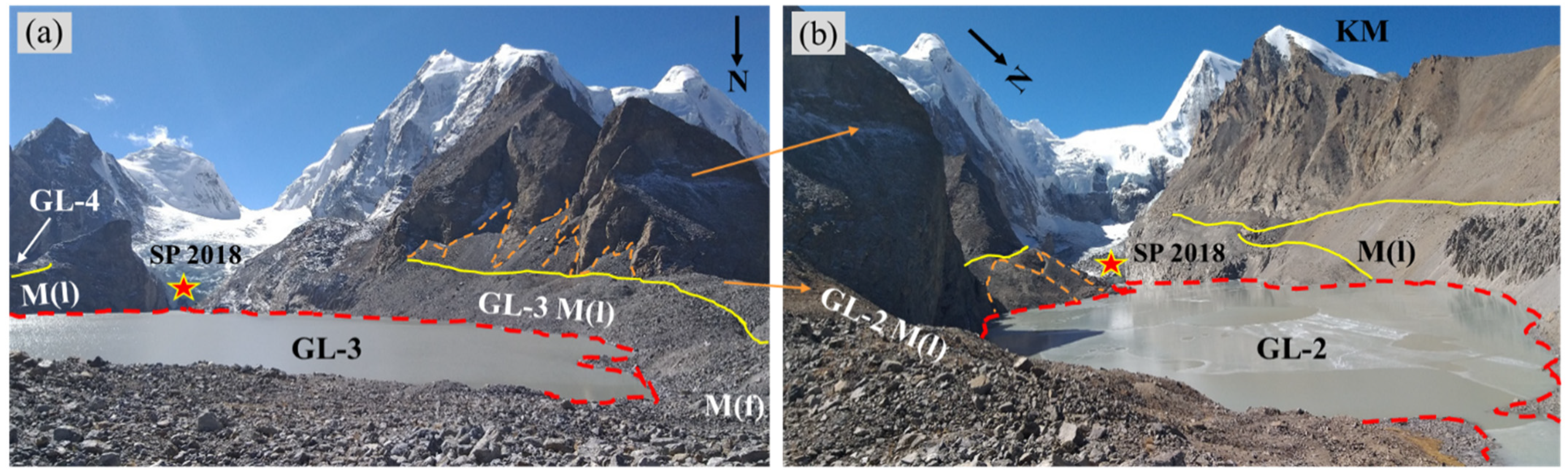
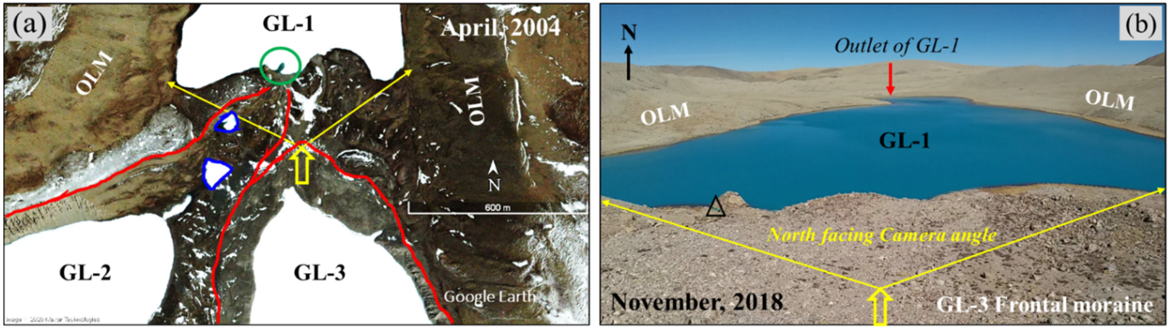
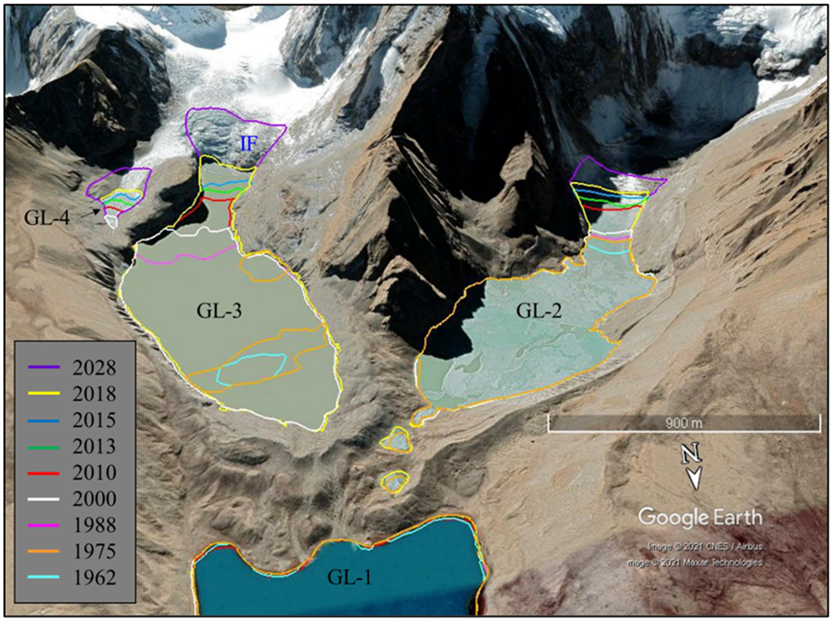
4.1. Geomorphological Description from Satellite Images and Field Investigation

Slopes in the close surroundings of the GLC were carved by fluvial erosion and slope movements. The older moraine of GL-1 is relatively smooth, and its frontal part is entirely missing, probably due to a paleo-outburst. Only remnants of lateral moraines are still present. The current outflow is curved into the large outwash cone (Figure 1c and Figure 3a,b). The morphological situations of GL-2 and GL-3 are significantly different, where the deglaciation is relatively recent (Figure 2); according to their shape they could be from the Little Ice Age. The fontal moraine of both lakes is common; nevertheless, some differences are visible. GL-2 is drained via a group of thermokarst lakes after melting of dead ice in the moraine, without any signs of recent dam overflow (Figure 3a). The non-frozen portion near the inlet of GL-1 directly suggests the issue of shallow subsurface drainage, i.e., visible on the satellite image of 2004 in the GE platform (Figure 3a). Two different glacier retreat steps are visible on the left lateral moraine of GL-2 without any evident changes after 2004. The posterior part of this lake was still glaciated during 1962 and attached to a large proglacial lake with an area of 0.82 ± 0.01 km². The situation around GL-3 is somewhat different. While observing the glacier reaction of Gurudongmar Khangse during 1962 using the KH-4 image, we found that GL-3 had not yet been formed in its current position within the study area. GL-3 has been transformed from supraglacial lakes into a proglacial lake, and the frontal moraine bears signs of lake water overflow from the past (but not after 2004). Neither remote sensing data nor field inspections found any small lakes, springs, or wetlands in this part of the frontal moraine. Since the water level of GL-3 does not grow after continuing glacier melting, seepage through the moraine must exist, but we have not found any surface flow in the field. Further, a small lake GL-4 was formed around 2000, and it seems that the water accumulated behind a dam created from bedrock and the right-lateral moraine of GL-3.

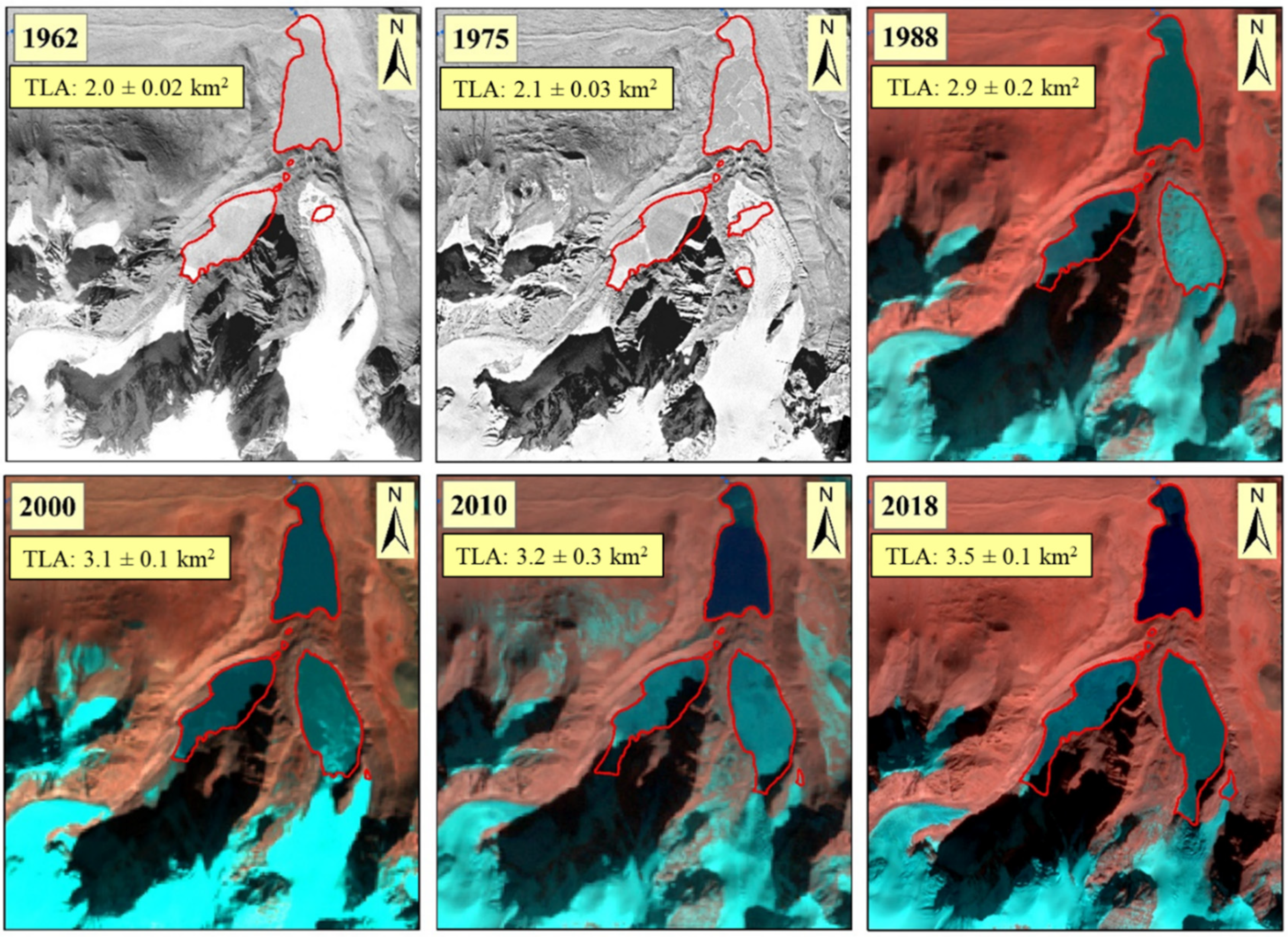
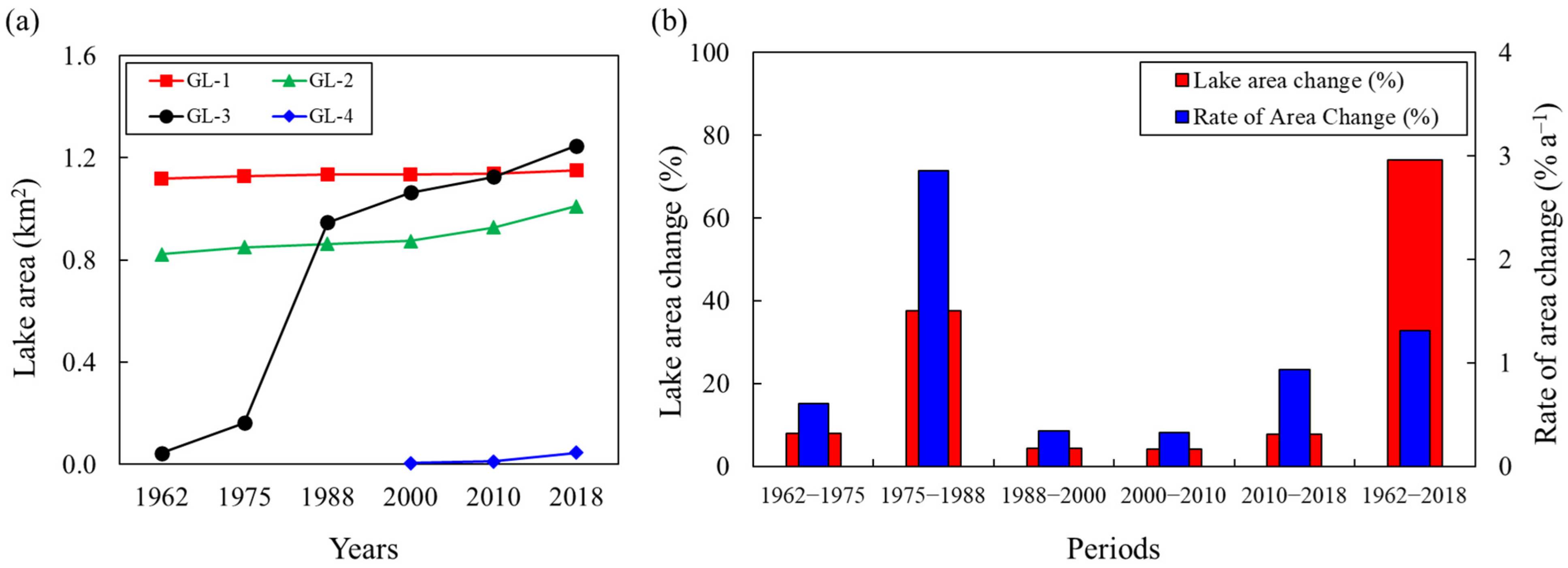
4.2. Spatio–Temporal Changes of GLC

Our results suggest that the area of GLC has increased over the past 43 years. The total lake area increased from 2.0 ± 0.02 km² (1962) to 3.5 ± 0.1 km² (2018), an increase of 1.5 ± 0.1 km² (~74.0 ± 3.0%). We have calculated the overall rate of lake area change as +0.03 ± 0.002 km² a⁻¹ (~+1.31 ± 0.05% a⁻¹) for the period 1962–2018. The total lake development rate varied across the studied timeframes, which showed an initial expansion rate of +0.01 ± 0.002 km² a⁻¹ between 1962 and 1975. During the period 1975–1988, the rate of change increased to +0.06 ± 0.02 km² a⁻¹ and later decreased to +0.01 ± 0.02 km² a⁻¹ during the period 1988–2000. This rate remained stable (i.e., +0.01 ± 0.03 km² a⁻¹) during the period 2000–2010. Again, the rate of change increased and reached +0.03 ± 0.03 km² a⁻¹ during the recent period 2010–2018. Figure 4 presents the spatio-temporal changes of the lake boundaries. From Figure 5a, the variations in the individual lake area during 1962–2018 can be seen very clearly. A newly formed proglacial lake (i.e., GL-4) has been observed since 2000, hanging over GL-3 (see Figure 4 and Figure 5a). During 1962, there was evidence of a small supraglacial lake formation, i.e., GL-3 gradually turned into two large supraglacial lakes observed during 1975. These supraglacial lakes formed into a proglacial moraine–dammed lake, which has grown tremendously over the years until the present (Figure 4). During 1962–2018, the GL-3 expanded more rapidly than any other GLC lake. Its area increased by +1.20 ± 0.03 km², at rates of 0.022 ± 0.001 km² a⁻¹, turning into a very dangerous overhanging large proglacial lake (Figure 5a), creating very high pressure on GL-1 for a potentially imminent GLOF event. Figure 5b shows the relative total lake area changes over the different timeframes.

It is quite evident from the comparative study of different satellite images from 1962, 1975, 1988, 2000, 2010, and 2018 that a higher magnitude of deglaciation has resulted in faster expansion of GLC over the past decades. Several other Himalayan proglacial moraine-dammed lakes have been expanding similarly due to associated glacier retreats [65,66,67].

4.3. GLC’s Volume Estimation

After using all formulae described above, differences between each volume estimation method can be seen (

Table 5. Results of volume estimation and means were used in the study for Emmer and Vilímek [54] methodology.

Adopted Methods for Volume Estimation	* Lake Volumes (m3 × 106)
	GL-1	GL-2	GL-3	GL-4
Huggel et al. [51]	42.10	34.93	47.13	0.42
Liu et al. [52]	45.92	37.85	51.60	0.40
Sharma et al. [25]	61.66	52.82	67.70	1.37
Mean	49.89	41.87	55.48	0.73

* Note: All the lake area calculations were based on Sentinel 2A MSI image (2018). All formulae are given in Table 2.

); thus, the mean volume was calculated. From the results, it is evident that the three lakes are very similar, each containing a relatively high volume of water. Each of them are potentially very dangerous when a GLOF occurs and together present a threat to the downstream areas of the Tista basin in Sikkim Himalaya.

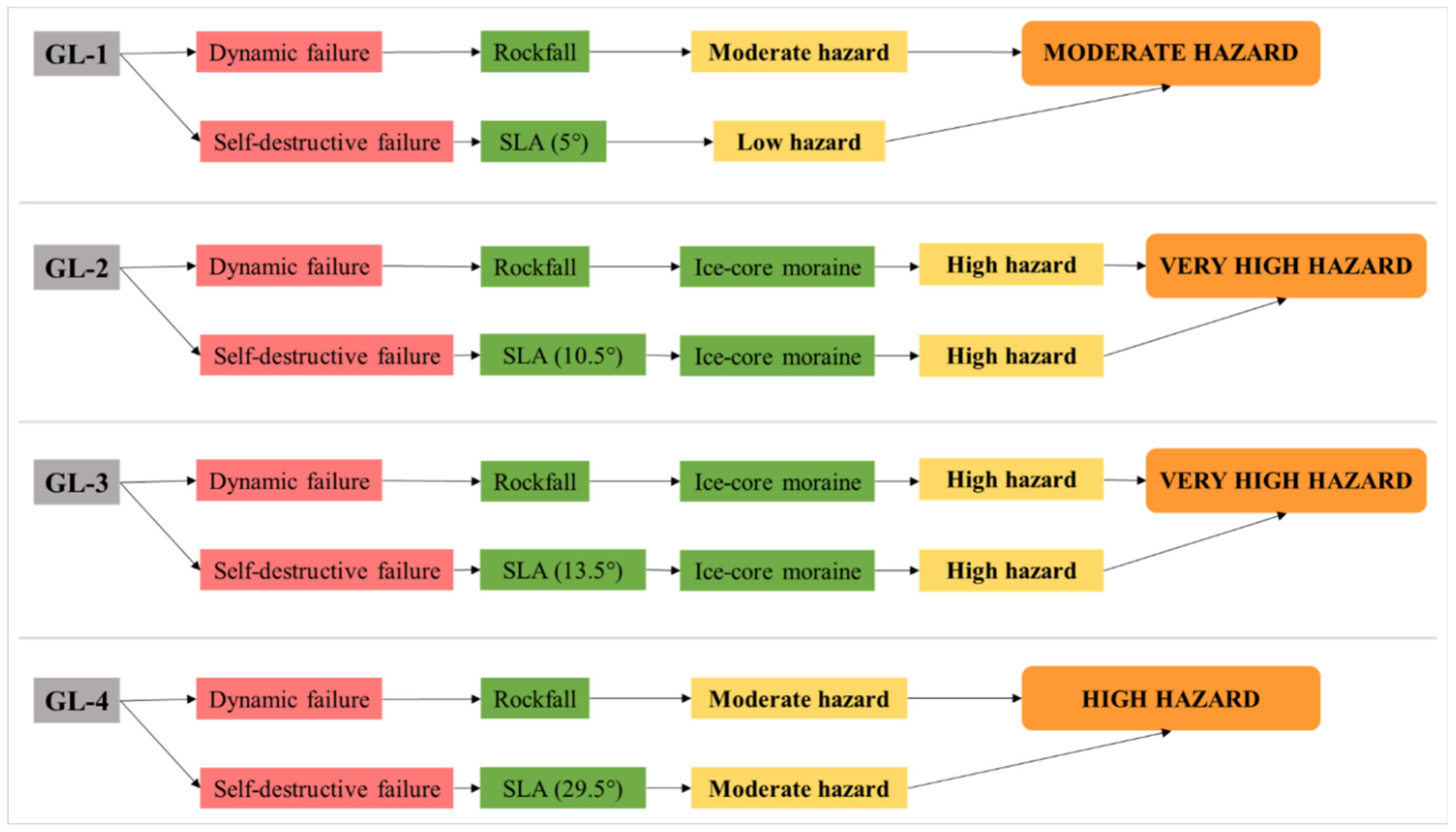
4.4. Susceptibility to Outburst Floods

The Gurudongmar lake complex is described as a cascade system or paternoster lake system, where an event on one lake can influence the downstream located lake, the stability of a dam, or produce dam overflow. To understand this system as one complex, it is first necessary to assess susceptibility to GLOF for each lake separately. Therefore, lake outburst susceptibility modelling is discussed in the following subsections from the highest to the lowest located lake, starting from GL-4 to GL-1, according to the mean elevation of the individual lake and its gradient of runoff pathways. The GLOF hazard of the whole complex of Gurudongmar lakes was evaluated by three different methodologies using different parameters. The results for each observed parameter of each lake is given in

Table 6. Results of observed parameters of each method used in GLOF hazard assessment.

Methodology	Observed Parameters	GL-1	GL-2	GL-3	GL-4
Method 1	mother glacier area (km2)	–	3.9	1.38	0.71
	distance between lake and glacier terminus (m)	–	0	0	0
	slope between lake and glacier (°)	–	–	–	–
	mean slope of moraine dam (°)	–	10.5	13.5	29.5
	mother glacier snout steepness (°)	–	7	13	9
Method 2	dam type	moraine and bedrock	moraine	moraine	moraine
	dam freeboard (m)	0	3	5	4
	dam width (m)	427	466	602	100
	dam height (m)	68	25	102	53
	maximum slope of distal face of the dam (°)	10.5	14.5	16.7	39.5
	piping	no	yes	yes	no
	piping gradient (°)	–	10	19.1	–
	remedial work	no	no	no	no
	lake area (m2)	1,152,000	1,010,000	1,247,000	45,000
	lake perimeter (m)	5430	6245	5923	1050
	maximum lake width (m)	942	769	853	229
	distance between lake and glacier (m)	–	0	0	0
	width of calving front (m)	–	430	351	102
	mean slope between lake and glacier (°)	–	–	–	–
	mean slope of last 500 m of glacier tongue (°)	–	15	19.5	14.7
	maximum slope of slopes surrounding lake (°)	44.5	74.6	67.4	42.1
	mean slope of lake surrounding (°)	15.8	30.8	21.8	17.9
	volume (m3 × 106)	49.89	41.87	55.48	0.73
Method 3	snow/ice avalanche	no	no	no	no
	rockfall	yes	yes	yes	yes
	GLOF upstream	yes	no	yes	no
	SLA (°)	5 (yes)	10.5 (yes)	13.5 (yes)	29.5 (yes)
	ice-cored moraine	no	yes	yes	no
	future change to hazards	no	yes	yes	yes

.

4.4.1. Susceptibility to Outburst of GL-4

This is the smallest and most newly-formed glacial lake in the study area (Figure 4). Even though it is small, Method 1 peaks for this glacial lake as it has a high potential to outburst; the same is true for Method 3, where the hazard is also high.

Using Method 2, there are three possible scenarios. This method assumes the occurrence of dam overtopping resulting from fast slope movement into the lake (Scenario 1) mainly due to small dam freeboard and a high potential for a landslide or rockfall into the lake. As with GL-2 and GL-3, dam failure resulting from fast slope movement into the lake (Scenario 3) is predicted there. Scenario 5, caused by an earthquake due to the high dam height to width ratio, has been calculated as possible, while the study area lies in a seismically active region [39,40].

Even though this is the lake with the highest potential to outburst, it should not influence other glacial lakes located downstream due to the high retention potential of GL-3 (calculated in Method 2) compared to a relatively limited amount of water available from GL-4.

4.4.2. Susceptibility to Outburst of GL-3

GL-3 had very similar results to GL-2 after using all three methods even though this lake has been formed recently compared to GL-2 (Figure 1c). Both these lakes have similar parameters, so there is also a probability of occurrence of Scenario 1 and Scenario 3 for Method 2. There is also a moderate potential to outburst when calculating Method 1. We also predict ice-cored damming moraine, so after applying flow chart 3, there is a very high potential hazard of GLOF from GL-3.

4.4.3. Susceptibility to Outburst of GL-2

GL-2 has been evaluated by all three methods mentioned above, and the results of each method vary (see

Table 7. Results from three different methodologies for outburst susceptibility used in this study.

Lakes	Method 1	Method 2	Method 3
GL-1	x	2/5	moderate
GL-2	0.5238 (middle)	2/5	very high *
GL-3	0.5788 (middle)	2/5	very high *
GL-4	0.7813 (high)	3/5	High *

* These results are derived from Sentinel 2A MSI image (2018) and GE platform which may change due to glacier retreat and glacial lakes enlarging.

). Method 1 indicates that the occurrence of GLOF is moderately probable (middle hazard was calculated) due to different weights of each parameter in this methodology—the mother glacier area, the distance between the lake and glacier terminus, and the slope between lake and glacier in the highest danger value category, while the mean slope of moraine dam and mother glacier snout steepness are located on the lowest, and second-lowest danger values, respectively.

Using Method 2, we observed that two scenarios of GLOF could occur on this glacial lake. Due to very steep slopes around the lake, a landslide or rockfall could cause an impact wave and overtop the moraine dam, e.g., Scenario 1. While there is no surface outflow, dam failure resulting from fast slope movement into the lake (Scenario 3) could occur. As with GL-1, this method indicates that GL-2 is very susceptible to outburst.

There is also a very high hazard after using Method 3, caused by rockfall prone slopes around the lake, ice-cored moraine (we expect dead ice in the moraine as there are very similar thermokarst lakes to moraines where the existence of dead ice was confirmed [68,69,70]), and SLA greater than 10°.

4.4.4. Susceptibility to Outburst of GL-1

As the glaciers retreated, this lake was the lowest and the oldest one formed in this lake complex. It is the only lake with a clear surface outflow and without direct contact with the glacier tongue. This lake was evaluated only by Method 2 and 3 (as mentioned above), and the results were different.

Using Method 2, we observed two scenarios that could occur (Table 7). The first is Scenario 1 with potential for dam overtopping resulting from fast slope movement into the lake. It is possible because there are slopes where landslides can occur and there is no dam freeboard (because of surface outflow), so the dam could be overtopped easily. We also have to consider the possibility of GLOF, which can occur from lakes situated upstream (Scenario 2). All other lakes located upstream were evaluated, inter alia, as susceptible to Scenario 1. There are three other glacial lakes located upstream that can cause a GLOF from the GL-1 after overtopping their dams because there is then the potential for retention of more water coming from lakes situated upstream. Method 2 evaluates the hazard as very high even though there is only one scenario possible, so we can say that GL-1 is very susceptible to outburst using this methodology.

Using Method 3, there is a moderate hazard to dynamic failure of the dam after rockfall/landslide coming from surrounding slopes while there is no dead ice in the damming moraine. The self-destructive failure is predicted with low hazard possibility, so when the risks are considered together, there is a moderate hazard to GLOF from GL-1 using this method (Figure 6).

4.4.5. Susceptibility Assessment Overview

We have assessed four separate lakes to evaluate the hazard of occurrence of GLOF in the Gurudongmar lake complex. After using the three different methodologies described above, each of these lakes was determined to have a moderate to very high potential to outburst. As we observed from our field investigations, the frontal dam near the outlet of GL-1 is breached (i.e., no dam structure); therefore, GL-1 does not provide any retention capacity. Hence, there is a very high potential for the whole complex to outburst with the sudden failure of any of the moraine-dammed lakes located upstream.

4.5. Influence of Climatological Changes on the Evolution of GLC

The Sikkim Himalaya, a part of the Eastern Himalayas, has four seasons: spring, summer, autumn, and winter. To understand the expansion of GLC and its susceptibility to glacial lake outburst floods, it is necessary to evaluate the trend analysis and detection of change in temperature and precipitation [70,71]. For this purpose, Mann–Kendall’s tau trend and Sen’s slope analyses of the season-wise temperature and precipitation for the period of 1960 to 2019 were performed (

Table 8. Mann–Kendall test for statistical trend analysis of long-term temperature and precipitation over the period 1960–2019. Sen’s Slope (Q) analysis shows the rate of change in temperature (°C a⁻¹) and precipitation (mm a⁻¹).

Seasons/Annual	Temperature				Precipitation
	Kendall’s Tau	p–Value (Two–Tailed)	Trend	Sen’s Slope	Kendall’s Tau	p–Value (Two–Tailed)	Trend	Sen’s Slope
				(°C a−1)				(mm a−1)
Spring	0.290	0.001	↑ *	0.054	0.232	0.009	↑ *	0.969
Summer	0.425	<0.0001	↑ *	0.060	−0.020	0.823	↓	−0.210
Autumn	0.298	0.001	↑ *	0.045	0.061	0.495	↑	0.159
Winter	0.401	<0.0001	↑ *	0.075	0.046	0.610	↑	0.063
Annual	0.527	<0.0001	↑ *	0.224	0.089	0.317	↑	1.119

Where, Spring (Pre-monsoon: Mar–May), Summer (Monsoon: Jun–Sep), Autumn (Post-monsoon: Oct–Nov), Winter (Dec–Feb); (↑), increasing trend; (↓), decreasing trend; * statistically significant at 0.05 alpha level of significance.

). All the seasonal temperatures and the corresponding annual temperature show a warming trend at a significant level. In contrast, the average annual precipitation and the precipitation for each season, except for spring, did not show any significant trend. The Mann-Kendall tau value, p-value, and Sen’s slope analysis show that spring was the only season experiencing an increasing precipitation trend at a 95% confidence level. The summer season’s precipitation showed a decreasing trend (−0.210 mm a⁻¹) but which was not statistically significant. The nature of the decreasing precipitation trend during summer and the warming air temperature over the year restricts the formation of solid ice [72] and has resulted in rapid areal expansion of GLC since 1962.

The PAI graphs (Figure 7) for the various seasons are consistent with the result derived through Mann-Kendall’s tau. The scarcity in the pre-monsoon season’s (spring) precipitation is visually apparent from 1960 to 1995, but with a sharp increase (>+2.0) evident from 1996 onwards. The summer season’s precipitation was highly variable over the period, except for a higher magnitude (<−2.0) negative anomaly observed from 1980 to 1995. A general deficit in autumn precipitation was observed with several sudden extreme positive anomalies up to 1990. The deficit in winter precipitation from 1960 to 1975 was replaced by excess precipitation from 1976 to 2004. Simultaneously, annual temperature variability (Figure 7) showed a positive trend with a higher frequency of warmer conditions. The positive departures of annual temperature from the normal were very frequent from 1998. Temperature variability for the other seasons also showed a similar increasing trend as for annual temperature variability. Positive anomalies of temperature for the autumn and winter seasons was very frequent from 1998 onwards. In contrast, positive anomalies of spring temperature were more frequent from 1980 to 2010. The summer season’s temperature showed continuous positive anomalies from 2005 to 2019.

The initial higher rate of areal expansion of GLC from 1962 to 1988 (+0.01 ± 0.002 km² a⁻¹ to +0.06 ± 0.02 km² a⁻¹) (see Figure 5b) was possibly triggered by the early phase of deficit in precipitation during winter and spring seasons. The post-1990s positive anomaly in precipitation might have reduced the rate of the glacial lake area expansion considerably. Hence, the overall area expansion rates of GLC were dependent on climate-driven factors.

5. Discussion

5.1. Comparison of Lake Changes in the Frame of Eastern Himalayas

The current study showed a significant GLC area change of +1.5 ± 0.1 km² (~74.0 ± 3.0%) with an expansion rate of +0.03 ± 0.002 km² a⁻¹ (~1.31 ± 0.05% a⁻¹) from 1962 and 2018. The development of individual lakes of GLC was not consistent (see Figure 5a). GL-1 had a static growth rate. GL-2 reached its maximum expansion rate before 1962, and now no significant changes are expected because an abrupt mountain cliff face topography bounds its upper extent. In contrast, the mother glacier of GL-3 (i.e., Gurudongmar Khangse) began to retreat significantly later [19]. This retreat is probably due to the larger accumulation area of the glacier and its greater thickness and speed. Therefore, the glacier began to respond to climate change later. Further, the mechanism of ice-calving into the GL-3 could have been the key reason for the faster lake growth in the upper part of the glacial area after 1962 [19]. The decrease in annual precipitation, as well as decrease in the spring, summer, and autumn precipitation, was evident during 1980–1985, and constantly increasing annual average temperature (Figure 7) together with this might have stimulated the retreat of the parent glacier of GL-3.

Figure 8 shows a comparatively higher rate of glacial lake area expansion (between 0.058 to 0.071 km² a⁻¹) in Bhutan than in another region of Eastern Himalayas. At the same time, the lake area development of GLC kept a similar pace (around 0.026 km² a⁻¹) to that of some other potentially dangerous glacial lakes (PDGLs) of Central Tibet (Longbasaba), northwest Sikkim (South Lhonak), and Nepal (i.e., Imja, Lumding and Tso Rolpa).

The higher rate of glacier area loss in the Eastern Himalayan region led to the growth of these PDGLs, which reflects the nature of climate warming and variability in the ISM as well as dominating mid-latitude westerlies during winters [42,78], independently of Karakoram and western Himalayas [79]. Another reason for the higher rate of expansion of north-facing (including northwest and northeast) lakes, such as GLC and Longbasaba, is the higher magnitude of glacier retreat because of more incident solar radiation [80] and increasing lake surface temperature [22].

5.2. Lake Volumes Estimation

Estimating lake volume is a very problematic step in any GLOF hazard assessment analysis for glacial lakes. Lakes are very often located in inaccessible areas, and so it is necessary to resort to the use of empirical formulae. The formulae chosen for this analysis are two globally used formulae [51,52] combined with a formula developed specifically for the Sikkim Himalayan region [25]. Due to the large uncertainties within each formula (see [81]) the resulting volumes were averaged, from which the final volume for each lake was derived. There would have been a significant refinement of the results if in-situ bathymetry had been performed, however, this was not possible for several reasons. The use of more than one method would probably not have led to a better result, hence three formulae were used.

5.3. Analysis of Outburst Susceptibility Assessment of GLC

The entire Gurudongmar lake complex was assessed based on three chosen methodologies to cover the maximum possible range of input parameters so that all potential GLOF triggers were included in the analysis. Each of the methods yielded quite different results due to the different input parameters (see Table 6). Several possible uncertainties affect assessment of the susceptibility to outburst of individual lakes in the Gurudongmar glacial lakes complex. Slight uncertainty arose during the initial mapping of the area of the lakes (see Section 3.2). However, the uncertainties in the exact area of the lakes should not affect the final assessment of the susceptibility to outburst/overflow. Another source of inaccuracy may be use of the global SRTM DEM model to calculate the slope, dam geometry, lake level, etc. The analysis of outburst susceptibility was performed using three different methodologies to ensure better and more detailed results. Since each method has different parameters put into the process of evaluation, it is necessary to compare the uncertainties of each.

The first method created by Wang et al. [53] (Method 1) provides an easily applicable analysis based on remote sensing data. Thus, it is a suitable tool for initial analysis even with a more significant number of studied lakes. However, compared with other quantitative methods, many parameters influencing the susceptibility to outburst/overflow are neglected. It can thus produce relatively inaccurate results. GL-1 was omitted from the analysis using this methodology as it is no longer in direct contact with the parent glacier, and the results from any analysis would be highly misleading. The results for GL-2 and GL-3 were very similar using this methodology, mainly because their input parameters to the analysis were also very similar. In particular, the occurrence of dead ice is neglected in this methodology, which may be a problem; however, dead ice melting was accounted for in the other analyses. GL-4 appears to be the most dangerous according to Method 1, mainly because it is very young, and the average slope of its dam is higher than that of GL-2 and GL-3.

The semi-quantitative method of Emmer and Vilímek [54] (Method 2) was used to provide a more comprehensive view of the entire system of studied lakes. Although this method was developed primarily for the Cordillera Blanca, it is widely used across all glaciated areas. However, other potential rupture triggers are not included in the method (for example, dead ice in a damming moraine, which can significantly impact the stability of a moraine dam). This method rates a lake as susceptible to outburst as soon as one of five possible scenarios can occur. Therefore, GL-1 is rated as hazardous because two scenarios are considered as possible for GLOF from a lake situated upstream (i.e., breaching and overtopping of the dam).

The last used method of Rounce et al. [55] (Method 3) was developed in the Nepalese Himalayas and should objectively include all potential triggers of GLOFs. However, it is quite significantly influenced by the complexity of the input data (the occurrence of dead ice here was confirmed based on a subjective evaluation by an expert from satellite data). Compared to Method 2, this method uses fewer input parameters; however, given the potential GLOF triggers in the Gurudongmar lake complex, this method should yield the best results when assessing individual lakes in the complex. It includes all potential triggers such as slope movements, avalanches, dead ice melting, or hydrostatic pressure increasing due to lake area growth.

It is not possible to state which of the methodologies is optimal for the assessment of this complex, as Method 1 mainly considers the parameters of the parent glacier, Method 2 does not include the melting of dead ice, and Method 3 does not consider the possibility of flooding from a lake located upstream. For this reason, it is therefore important to look at the complex using different methods and to assess it holistically.

5.4. Future Possible Evolution of GLC

In Sikkim Himalaya, a recent study by Chowdhury et al. [19] showed that the mother glacier of GL-3 and GL-2 had an area loss of −1.1 ± 0.06% a⁻¹ and −0.2 ± 0.05% a⁻¹ over the period between 1975 and 2018. This inconsistent rate of glacier melting and calving processes played a dominant role in individual lake area enlargement over the years. We can expect future enlargement of GL-3 and GL-4 due to glacial tongue retreat, while space for enlargement of GL-2 is somewhat limited. We also need to consider that prolonging the lake is one issue, but the lake volume can grow even more quickly because the hard rock basin is usually deeper in the back of the lake rather than in the frontal part (close to the frontal moraine). It means that proper hazard management will be of high importance to keep the water level in safe conditions. An example of successful remedial measures can be seen in the Cordillera Blanca (Peru), where almost 40 lakes were described as implementing different structural measures [82]. GL-1 is already without any contact with current glaciation; nevertheless, it is strongly connected with the upstream glacial lakes from the GLC.

The lakes extent velocity from the previous year was used for basic future evolution estimation. The mean velocity from the last ten years shows that GL-2 will reach the maximum of its area in the next ten years because the steep surrounding slopes around lakeshores and glacier terminus will also reach the slopes. In contrast, GL-3 will probably continue to enlarge its area due to the continuing retreat of its mother glacier due to active calving processes of crevasses [83]. The current smaller lake in the GLC (i.e., GL-4) is constantly growing, and both the area of the clean and debris-covered part of its mother glacier is losing its glacier mass. GL-1 will probably remain the same, as it is not connected to the current termini. The estimated possible areas of GL-2, GL-3, and GL-4 in 2028 are 1.12 km², 1.50 km², and 0.12 km², respectively (Figure 9).

In the Gurudongmar region, the average annual temperature showed a significant increasing (positive) trend at a rate of 0.224 °C a⁻¹ (0.05 significance level) between 1960–2019 (See Table 8), which is much higher than the entire Hindu Kush Himalaya region average annual temperature rate of 0.104 °C per decade during 1901–2014 [84] and the global average temperature rate of 0.0074 °C a⁻¹ [85]. The linear regression dash green line with R² value of 0.49 for annual temperature variability over 1960–2019 in Figure 7 also illustrates the increasing trend. If the temperature follows the same rate of increase in the Gurudongmar semi-arid region, then within the next ten years (i.e., 2028), the crevasses formed at the steep terrain near the icefall region of Gurudongmar Khangse (Figure 9) will shrink due to enhanced melting and calving processes as a result of differences in the outward cryostatic pressure (i.e., the pressure exerted by ice) and inward hydrostatic pressure (i.e., the pressure exerted by water) near the current terminus of GL-3 [86]. Calving may also occur by frontward collapse of overhanging ice blocks as a result of the continuous development of thermo-erosional notches cut into the terminal ice cliff due to faster heat transfer from large proglacial lakes, such as GL-2 and GL-3 [87].

6. Conclusions

In this study, we have analysed the evolution and changes in the area of Gurudongmar lake complex from 1962–2018 and estimated the future lake complex evolution up to 2028. This study also assessed and predicted the probability of individual lake susceptibility to outburst floods. Spatio-temporal change analysis between 1962 and 2018 revealed a total lake area increase of 74.0 ± 3.0%, with an expansion rate of +1.31 ± 0.05% a⁻¹. The development of GLC was inconsistent throughout different timeframes, such as during 1975–1988 when the lake area expansion rate was maximum with +2.9 ± 0.7% a⁻¹ due to the deficit in winter and spring precipitation, as well as overall warming temperature, without considering the lagging period. Later the rate expansion decreased. Again from 2000 onwards, the rate of expansion increased as a result of continuous deglaciation in this catchment induced by climate warming. Among all other lakes, GL-3 showed a considerable maximum amount of lake area expansion of +1.20 ± 0.03 km², with a rapidly increasing rate of 0.022 ± 0.001 km² a⁻¹ since 1962 as a result of the interplay of topography and climate change in this study region.

To assess glacial lake outburst susceptibility, glacial lake volume estimation is a key input. In 2018, the empirically calculated mean lake volumes of GL-1, GL-2, GL-3, and GL-4 were 49.9, 41.9, 55.5, and 0.7 m³ × 10⁶, respectively, with a huge total water storage capacity of 148 m³ × 10⁶ indicating the possible development of GLOF hazard scenario in the valley. As a result, this outburst susceptibility assessment revealed that the whole complex has a very high potential hazard to outbursts or overflow. The hazard susceptibility analysis showed that the glacial lakes GL-2, GL-3 and GL-4 in the system are highly GLOF hazard-prone driven by inducing parameters such as slope movement into the lake, calving, earthquake, and melting of buried ice. Even though GL-1 has the lowest hazard for GLOF occurrence, the cascading effect of upstream lakes’ hazards probability and no retention capacity of GL-1, could lead to devastating hazards from this catchment. The future possible lake area expansion estimation further emphasises the gravity of the situation, considering that it has been found that the GL-2 and GL-3 areas will expand unprecedentedly (1.12 km² and 1.50 km², respectively) until 2028 under the special topographic circumstances.

References

1. Haeberli, W.; Huggel, C.; Paul, F.; Zemp, M. Glacial Responses to Climate Change. In Treatise on Geomorphology; Shroder, J., James, L.A., Harden, C.P., Clague, J.J., Eds.; Academic Press: San Diego, CA, USA, 2013; Volume 13, pp. 152–175. ISBN 9780123747396. [Google Scholar]
2. Shrestha, A.B.; Eriksson, M.; Mool, P.; Ghimire, P.; Mishra, B.; Khanal, N.R. Glacial lake outburst flood risk assessment of Sun Koshi basin, Nepal. Geomat. Nat. Hazards Risk 2010, 1, 157–169. [Google Scholar] [CrossRef]
3. Clague, J. Deglaciation of the Cordillera of Western Canada at the end of the Pleistocene. Cuad. Investig. Geográfica 2017, 43, 449. [Google Scholar] [CrossRef] [Green Version]
4. Emmer, A.; Vilímek, V.; Huggel, C.; Klimeš, J.; Schaub, Y. Limits and challenges to compiling and developing a database of glacial lake outburst floods. Landslides 2016, 13, 1579–1584. [Google Scholar] [CrossRef]
5. Costa, J.E.; Schuster, R.L. The Formation and Failure of Natural Dams; United States Geological Survey Vancouver: Washington, DC, USA, 1987.
6. Clague, J.J.; Evans, S.G. A review of catastrophic drainage of moraine-dammed lakes in British Columbia. Quat. Sci. Rev. 2000, 19, 1763–1783. [Google Scholar] [CrossRef]
7. ICIMOD. Glacial Lakes and Glacial Lake Outburst Floods in Nepal; ICIMOD: Kathmandu, Nepal, 2011. [Google Scholar]
8. Iturrizaga, L. Glacier lake outburst floods. In Encyclopedia of Snow, Ice and Glaciers. Encyclopedia of Earth Sciences Series; Singh, V.P., Singh, P., Haritashya, U.K., Eds.; Springer: Dordrecht, The Netherlands, 2011; pp. 381–399. ISBN 9789048126415. [Google Scholar]
9. Vilímek, V.; Klimeš, J.; Emmer, A.; Benešová, M. Geomorphologic impacts of the glacial lake outburst flood from Lake No. 513 (Peru). Environ. Earth Sci. 2014, 73, 5233–5244. [Google Scholar] [CrossRef]
10. Emmer, A.; Cochachin, A. The causes and mechanisms of moraine-dammed lake failures in the Cordillera Blanca, North American Cordillera, and Himalayas. AUC Geogr. 2013, 48, 5–15. [Google Scholar] [CrossRef] [Green Version]
11. Schmidt, S.; Nüsser, M.; Baghel, R.; Dame, J. Cryosphere hazards in Ladakh: The 2014 Gya glacial lake outburst flood and its implications for risk assessment. Nat. Hazards 2020, 104, 2071–2095. [Google Scholar] [CrossRef]
12. Owen, L.A.; Sharma, M.C.; Bigwood, R. Landscape modification and geomorphological consequences of the 20th October 1991 earthquake and the July-August 1992 monsoon in the Garhwal Himalaya. Zeitschrift für Geomorphol. 1996, 103, 359–372. [Google Scholar]
13. Barnard, P.L.; Owen, A.L.; Sharma, M.C.; Finkel, R.C. Natural and human-induced landsliding in the Garhwal Himalaya of northern India. Geomorphology 2001, 40, 21–35. [Google Scholar] [CrossRef]
14. Bajracharya, S.R.; Mool, P. Glaciers, glacial lakes and glacial lake outburst floods in the Mount Everest region, Nepal. Ann. Glaciol. 2009, 50, 81–86. [Google Scholar] [CrossRef] [Green Version]
15. Bajracharya, S.R.; Maharjan, S.B.; Shrestha, F. The status and decadal change of glaciers in Bhutan from the 1980s to 2010 based on satellite data. Ann. Glaciol. 2014, 55, 159–166. [Google Scholar] [CrossRef] [Green Version]
16. Aggarwal, S.; Rai, S.; Thakur, P.; Emmer, A. Inventory and recently increasing GLOF susceptibility of glacial lakes in Sikkim, Eastern Himalaya. Geomorphology 2017, 295, 39–54. [Google Scholar] [CrossRef]
17. Nie, Y.; Liu, Q.; Wang, J.; Zhang, Y.; Sheng, Y.; Liu, S. An inventory of historical glacial lake outburst floods in the Himalayas based on remote sensing observations and geomorphological analysis. Geomorphology 2018, 308, 91–106. [Google Scholar] [CrossRef]
18. Debnath, M.; Sharma, M.C.; Syiemlieh, H.J. Glacier Dynamics in Changme Khangpu Basin, Sikkim Himalaya, India, between 1975 and 2016. Geosciences 2019, 9, 259. [Google Scholar] [CrossRef] [Green Version]
19. Chowdhury, A.; Sharma, M.C.; De, S.K.; Debnath, M. Glacier changes in the Chhombo Chhu Watershed of the Tista basin between 1975 and 2018, the Sikkim Himalaya, India. Earth Syst. Sci. Data 2021, 13, 2923–2944. [Google Scholar] [CrossRef]
20. Racoviteanu, A.E.; Arnaud, Y.; Williams, M.W.; Manley, W.F. Spatial patterns in glacier characteristics and area changes from 1962 to 2006 in the Kanchenjunga–Sikkim area, eastern Himalaya. Cryosphere 2015, 9, 505–523. [Google Scholar] [CrossRef] [Green Version]
21. Bahuguna, I.M.; Rathore, B.P.; Brahmbhatt, R.; Sharma, M.C.; Dhar, S.; Randhawa, S.S.; Kumar, K.; Romshoo, S.; Shah, R.D.; Ganjoo, R.K.; et al. Are the Himalayan glaciers retreating? Curr. Sci. 2014, 106, 1008–1013. [Google Scholar]
22. Debnath, M.; Syiemlieh, H.J.; Sharma, M.C.; Kumar, R.; Chowdhury, A.; Lal, U. Glacial lake dynamics and lake surface temperature assessment along the Kangchengayo-Pauhunri Massif, Sikkim Himalaya, 1988–2014. Remote Sens. Appl. Soc. Environ. 2018, 9, 26–41. [Google Scholar] [CrossRef]
23. Kumar, B.; Prabhu, T.S.M. Impacts of climate change: Glacial Lake Outburst Floods (GLOFs). In Climate Change in Sikkim-Patterns, Impacts and Initiatives; Arrawatia, M.L., Tambe, S., Eds.; Information and Public Relations Department, GoS: Gangtok, India, 2012; pp. 81–102. ISBN 978-81-920437-0-9. [Google Scholar]
24. Sattar, A.; Goswami, A.; Kulkarni, A.V. Hydrodynamic moraine-breach modeling and outburst flood routing-A hazard assessment of the South Lhonak lake, Sikkim. Sci. Total Environ. 2019, 668, 362–378. [Google Scholar] [CrossRef]
25. Sharma, R.K.; Pradhan, P.; Sharma, N.P.; Shrestha, D.G. Remote sensing and in situ-based assessment of rapidly growing South Lhonak glacial lake in eastern Himalaya, India. Nat. Hazards 2018, 93, 393–409. [Google Scholar] [CrossRef]
26. Ives, J.D.; Shrestha, R.B.; Mool, P.K. Formation of Glacial Lakes in the Hindu Kush-Himalayas and GLOF Risk Assessment; ICIMOD: Kathmandu, Nepal, 2010. [Google Scholar]
27. Worni, R.; Huggel, C.; Stoffel, M. Glacial lakes in the Indian Himalayas—From an area-wide glacial lake inventory to on-site and modeling based risk assessment of critical glacial lakes. Sci. Total Environ. 2013, 468–469, S71–S84. [Google Scholar] [CrossRef]
28. Nie, Y.; Liu, Q.; Liu, S. Glacial Lake Expansion in the Central Himalayas by Landsat Images, 1990–2010. PLoS ONE 2013, 8, e83973. [Google Scholar] [CrossRef] [Green Version]
29. Wang, W.; Xiang, Y.; Gao, Y.; Lu, A.; Yao, T. Rapid expansion of glacial lakes caused by climate and glacier retreat in the Central Himalayas. Hydrol. Process. 2014, 29, 859–874. [Google Scholar] [CrossRef]
30. Zhang, G.; Yao, T.; Xie, H.; Wang, W.; Yang, W. An inventory of glacial lakes in the Third Pole region and their changes in response to global warming. Glob. Planet. Chang. 2015, 131, 148–157. [Google Scholar] [CrossRef]
31. Huggel, C.; Haeberli, W.; Kääb, A.; Bieri, D.; Richardson, S. An assessment procedure for glacial hazards in the Swiss Alps. Can. Geotech. J. 2004, 41, 1068–1083. [Google Scholar] [CrossRef]
32. Carrivick, J.; Tweed, F. Proglacial lakes: Character, behaviour and geological importance. Quat. Sci. Rev. 2013, 78, 34–52. [Google Scholar] [CrossRef] [Green Version]
33. Emmer, A.; Klimeš, J.; Mergili, M.; Vilímek, V.; Cochachin, A. 882 lakes of the Cordillera Blanca: An inventory, classification, evolution and assessment of susceptibility to outburst floods. CATENA 2016, 147, 269–279. [Google Scholar] [CrossRef]
34. Wilson, R.; Glasser, N.F.; Reynolds, J.M.; Harrison, S.; Anacona, P.I.; Schaefer, M.; Shannon, S. Glacial lakes of the Central and Patagonian Andes. Glob. Planet. Chang. 2018, 162, 275–291. [Google Scholar] [CrossRef]
35. Haritashya, U.K.; Singh, V.P.; Singh, P. Paternoster Lakes. In Encyclopedia of Snow, Ice and Glaciers. Encyclopedia of Earth Sciences Series; Singh, V.P., Singh, P., Haritashya, U.K., Eds.; Springer: Dordrecht, The Netherlands, 2011; p. 826. ISBN 9789048126422. [Google Scholar]
36. Neogi, S.; Dasgupta, S.; Fukuoka, M. High P-T Polymetamorphism, Dehydration Melting, and Generation of Migmatites and Granites in the Higher Himalayan Crystalline Complex, Sikkim, India. J. Pet. 1998, 39, 61–99. [Google Scholar] [CrossRef]
37. GSI. Geology and Mineral Resources of Sikkim; GSI: Kolkata, India, 2012.
38. Basu, S.K. Geology of Sikkim State and Darjeeling District of West Bengal, 1st ed.; Geological Society of India: Bangalore, India, 2013; ISBN 97893809980503. [Google Scholar]
39. Baruah, S.; Saikia, S.; Baruah, S.; Bora, P.K.; Tatevossian, R.; Kayal, J.R. The September 2011 Sikkim Himalaya earthquake Mw 6.9: Is it a plane of detachment earthquake? Geomat. Nat. Hazards Risk 2014, 7, 248–263. [Google Scholar] [CrossRef]
40. Rahman, M.M.; Bai, L.; Khan, N.G.; Li, G. Probabilistic Seismic Hazard Assessment for Himalayan–Tibetan Region from Historical and Instrumental Earthquake Catalogs. Pure Appl. Geophys. PAGEOPH 2017, 175, 685–705. [Google Scholar] [CrossRef]
41. Schmidt, S.; Nüsser, M. Changes of High Altitude Glaciers from 1969 to 2010 in the Trans-Himalayan Kang Yatze Massif, Ladakh, Northwest India. Arctic Antarct. Alp. Res. 2012, 44, 107–121. [Google Scholar] [CrossRef]
42. Benn, D.I.; Owen, L.A. The role of the Indian summer monsoon and the mid-latitude westerlies in Himalayan glaciation: Review and speculative discussion. J. Geol. Soc. 1998, 155, 353–363. [Google Scholar] [CrossRef] [Green Version]
43. Chand, P.; Sharma, M.C. Glacier changes in the Ravi basin, North-Western Himalaya (India) during the last four decades (1971–2010/13). Glob. Planet. Chang. 2015, 135, 133–147. [Google Scholar] [CrossRef]
44. Zhang, G.; Bolch, T.; Allen, S.; Linsbauer, A.; Chen, W.; Wang, W. Glacial lake evolution and glacier–lake interactions in the Poiqu River basin, central Himalaya, 1964–2017. J. Glaciol. 2019, 65, 347–365. [Google Scholar] [CrossRef] [Green Version]
45. Granshaw, F.D.; Fountain, A.G. Glacier change (1958–1998) in the North Cascades National Park Complex, Washington, USA. J. Glaciol. 2006, 52, 251–256. [Google Scholar] [CrossRef] [Green Version]
46. Bolch, T.; Menounos, B.; Wheate, R. Landsat-based inventory of glaciers in western Canada, 1985–2005. Remote Sens. Environ. 2010, 114, 127–137. [Google Scholar] [CrossRef]
47. Hall, D.K.; Bayr, K.J.; Schöner, W.; Bindschadler, R.A.; Chien, J.Y. Consideration of the errors inherent in mapping historical glacier positions in Austria from the ground and space (1893–2001). Remote Sens. Environ. 2003, 86, 566–577. [Google Scholar] [CrossRef]
48. Cook, S.; Swift, D. Subglacial basins: Their origin and importance in glacial systems and landscapes. Earth-Sci. Rev. 2012, 115, 332–372. [Google Scholar] [CrossRef] [Green Version]
49. Yao, X.; Liu, S.; Han, L.; Sun, M.; Zhao, L. Definition and classification system of glacial lake for inventory and hazards study. J. Geogr. Sci. 2018, 28, 193–205. [Google Scholar] [CrossRef] [Green Version]
50. Turconi, L.; Tropeano, D.; Savio, G.; De, S.K.; Mason, P.J. Landscape analysis for multi-hazard prevention in Orco and Soana valleys, Northwest Italy. Nat. Hazards Earth Syst. Sci. 2015, 15, 1963–1972. [Google Scholar] [CrossRef]
51. Huggel, C.; Kääb, A.; Haeberli, W.; Teysseire, P.; Paul, F. Remote sensing based assessment of hazards from glacier lake outbursts: A case study in the Swiss Alps. Can. Geotech. J. 2002, 39, 316–330. [Google Scholar] [CrossRef] [Green Version]
52. Liu, M.; Chen, N.; Zhang, Y.; Deng, M. Glacial Lake Inventory and Lake Outburst Flood/Debris Flow Hazard Assessment after the Gorkha Earthquake in the Bhote Koshi Basin. Water 2020, 12, 464. [Google Scholar] [CrossRef] [Green Version]
53. Wang, W.; Yao, T.; Gao, Y.; Yang, X.; Kattel, D.B. A First-order Method to Identify Potentially Dangerous Glacial Lakes in a Region of the Southeastern Tibetan Plateau. Mt. Res. Dev. 2011, 31, 122. [Google Scholar] [CrossRef]
54. Emmer, A.; Vilímek, V. New method for assessing the susceptibility of glacial lakes to outburst floods in the Cordillera Blanca, Peru. Hydrol. Earth Syst. Sci. 2014, 18, 3461–3479. [Google Scholar] [CrossRef] [Green Version]
55. Rounce, D.R.; McKinney, D.C.; Lala, J.M.; Byers, A.C.; Watson, C.S. A new remote hazard and risk assessment framework for glacial lakes in the Nepal Himalaya. Hydrol. Earth Syst. Sci. 2016, 20, 3455–3475. [Google Scholar] [CrossRef] [Green Version]
56. Bolch, T.; Peters, J.; Yegorov, A.; Pradhan, B.; Buchroithner, M.; Blagoveshchensky, V. Identification of potentially dangerous glacial lakes in the northern Tien Shan. Nat. Hazards 2011, 59, 1691–1714. [Google Scholar] [CrossRef] [Green Version]
57. Alean, J. Ice Avalanches: Some Empirical Information about their Formation and Reach. J. Glaciol. 1985, 31, 324–333. [Google Scholar] [CrossRef] [Green Version]
58. Shea, J.M.; Immerzeel, W.W.; Wagnon, P.; Vincent, C.; Bajracharya, S. Modelling glacier change in the Everest region, Nepal Himalaya. Cryosphere 2015, 9, 1105–1128. [Google Scholar] [CrossRef] [Green Version]
59. Harris, I.; Osborn, T.J.; Jones, P.; Lister, D. Version 4 of the CRU TS monthly high-resolution gridded multivariate climate dataset. Sci. Data 2020, 7, 1–18. [Google Scholar] [CrossRef] [Green Version]
60. Mann, H.B. Nonparametric Tests against Trend. Econometrica 1945, 13, 245–259. [Google Scholar] [CrossRef]
61. Kendall, M.G. Rank Correlation Methods, 4th ed.; Charles Griffin: London, UK, 1975. [Google Scholar]
62. Sen, P.K. Estimates of the regression coefficient based on Kendall’s Tau. J. Am. Stat. Assoc. 1968, 63, 1379–1389. [Google Scholar] [CrossRef]
63. Sreekesh, S.; Debnath, M. Spatio-Temporal Variability of Rainfall and Temperature in Northeast India. In Geostatistical and Geospatial Approaches for the Characterization of Natural Resources in the Environment; Raju, N.J., Ed.; Springer: Cham, Switzerland, 2016; pp. 873–879. ISBN 9783319186634. [Google Scholar]
64. Rooy, M.P. A Rainfall Anomaly Index (RAI), Independent of the Time and Space. Notos 1965, 14, 43–48. [Google Scholar]
65. Richardson, S.D.; Reynolds, J.M. An overview of glacial hazards in the Himalayas. Quat. Int. 2000, 65–66, 31–47. [Google Scholar] [CrossRef]
66. Thompson, S.S.; Benn, D.I.; Dennis, K.; Luckman, A. A rapidly growing moraine-dammed glacial lake on Ngozumpa Glacier, Nepal. Geomorphology 2012, 145–146, 1–11. [Google Scholar] [CrossRef]
67. Shijin, W.; Dahe, Q.; Cunde, X. Moraine-dammed lake distribution and outburst flood risk in the Chinese Himalaya. J. Glaciol. 2015, 61, 115–126. [Google Scholar] [CrossRef] [Green Version]
68. Hambrey, M.J.; Quincey, D.J.; Glasser, N.F.; Reynolds, J.M.; Richardson, S.J.; Clemmens, S. Sedimentological, geomorphological and dynamic context of debris-mantled glaciers, Mount Everest (Sagarmatha) region, Nepal. Quat. Sci. Rev. 2008, 27, 2361–2389. [Google Scholar] [CrossRef]
69. Janský, B.; Engel, Z.; Šobr, M.; Beneš, V.; Spaček, K.; Yerokhin, S. The evolution of Petrov lake and moraine dam rupture risk (Tien-Shan, Kyrgyzstan). Nat. Hazards 2008, 50, 83–96. [Google Scholar] [CrossRef]
70. Kroczek, T.; Vilímek, V. Rockfall/Rockslide Hazard, Lake Expansion and Dead-Ice Melting Assessment: Lake Imja, Nepal. In Understanding and Reducing Landslide Disaster Risk; Vilímek, V., Wang, F., Strom, A., Sassa, K., Bobrowsky, P.T., Takara, K., Eds.; Springer: Cham, Switzerland, 2021; pp. 103–110. ISBN 9783030603182. [Google Scholar]
71. Prakash, C.; Nagarajan, R. Outburst susceptibility assessment of moraine-dammed lakes in Western Himalaya using an analytic hierarchy process. Earth Surf. Process. Landf. 2017, 42, 2306–2321. [Google Scholar] [CrossRef]
72. Benn, D.I.; Wiseman, S.; Hands, K.A. Growth and drainage of supraglacial lakes on debris-mantled Ngozumpa Glacier, Khumbu Himal, Nepal. J. Glaciol. 2001, 47, 626–638. [Google Scholar] [CrossRef] [Green Version]
73. Mool, P.; Wangda, D.; Bajracharya, S.R.; Kunzang, K.; Gurung, D.R.; Joshi, S.P. Inventory of Glaciers, Glacial Lakes, and Glacial Lake Outburst Floods: Monitoring and Early Warning Systems in the Hindu Kush-Himalayan Region, Bhutan; ICIMOD (International Centre for Integrated Mountain Development): Kathmandu, Nepal, 2001; pp. 1–254. ISBN 9291153451. [Google Scholar]
74. Singh, S.M. The Cost of Climate Change: The Story of Thorthormi Glacial Lake in Bhutan; WWF: Gland, Switzerland, 2009; pp. 1–32. [Google Scholar]
75. Yao, X.; Liu, S.; Sun, M.; Wei, J.; Guo, W. Volume calculation and analysis of the changes in moraine-dammed lakes in the north Himalaya: A case study of Longbasaba lake. J. Glaciol. 2012, 58, 753–760. [Google Scholar] [CrossRef] [Green Version]
76. Somos-Valenzuela, M.A.; McKinney, D.C.; Rounce, D.R.; Byers, A.C. Changes in Imja Tsho in the Mount Everest region of Nepal. Cryosphere 2014, 8, 1661–1671. [Google Scholar] [CrossRef] [Green Version]
77. Thakuri, S.; Salerno, F.; Bolch, T.; Guyennon, N.; Tartari, G. Factors controlling the accelerated expansion of Imja Lake, Mount Everest region, Nepal. Ann. Glaciol. 2016, 57, 245–257. [Google Scholar] [CrossRef] [Green Version]
78. Ageta, Y.; Higuchi, K. Estimation of Mass Balance Components of a Summer-Accumulation Type Glacier in the Nepal Himalaya. Geogr. Ann. Ser. A Phys. Geogr. 1984, 66, 249–255. [Google Scholar] [CrossRef]
79. Bhambri, R.; Bolch, T.; Chaujar, R.K.; Kulshreshtha, S.C. Glacier changes in the Garhwal Himalaya, India, from 1968 to 2006 based on remote sensing. J. Glaciol. 2011, 57, 543–556. [Google Scholar] [CrossRef] [Green Version]
80. Evans, I.S. Local aspect asymmetry of mountain glaciation: A global survey of consistency of favoured directions for glacier numbers and altitudes. Geomorphology 2006, 73, 166–184. [Google Scholar] [CrossRef]
81. Cook, S.J.; Quincey, D.J. Estimating the volume of Alpine glacial lakes. Earth Surf. Dyn. 2015, 3, 559–575. [Google Scholar] [CrossRef] [Green Version]
82. Emmer, A.; Vilímek, V.; Zapata, M. Hazard mitigation of glacial lake outburst floods in the Cordillera Blanca (Peru): The effectiveness of remedial works. J. Flood Risk Manag. 2016, 11, S489–S501. [Google Scholar] [CrossRef]
83. Benn, D.; Warren, C.; Mottram, R.H. Calving processes and the dynamics of calving glaciers. Earth-Sci. Rev. 2007, 82, 143–179. [Google Scholar] [CrossRef]
84. Ren, Y.-Y.; Ren, G.-Y.; Sun, X.-B.; Shrestha, A.B.; You, Q.-L.; Zhan, Y.-J.; Rajbhandari, R.; Zhang, P.-F.; Wen, K.-M. Observed changes in surface air temperature and precipitation in the Hindu Kush Himalayan region over the last 100-plus years. Adv. Clim. Chang. Res. 2017, 8, 148–156. [Google Scholar] [CrossRef]
85. Mahmood, R.; Jia, S.; Zhu, W. Analysis of climate variability, trends, and prediction in the most active parts of the Lake Chad basin, Africa. Sci. Rep. 2019, 9, 1–18. [Google Scholar] [CrossRef] [Green Version]
86. Reeh, N. On The Calving of Ice From Floating Glaciers and Ice Shelves. J. Glaciol. 1968, 7, 215–232. [Google Scholar] [CrossRef] [Green Version]
87. Röhl, K. Thermo-erosional notch development at fresh-water-calving Tasman Glacier, New Zealand. J. Glaciol. 2006, 52, 203–213. [Google Scholar] [CrossRef] [Green Version]
Figure 1. Location of the study area: (a) Topographic map of Indian sub-continent showing the study site (identified in red circle) in Sikkim (inset in a dark black box), a part of Eastern Himalayas. Base map: World Shaded Relief map; (b) Enlarged location of the Gurudongmar lake complex (GLC) is shown within the district boundary of Sikkim state of India; (c) Extent of the GLC within the catchment extracted from Sentinel 2A MSI (2018) and SRTM DEM (2000). Note: KM, Kangchengyao massif; STDZ, South Tibetan Detachment Zone.
Water 13 03565 g001
Figure 2. Geomorphological characteristics of proglacial moraine-dammed lakes sites: (a) GL-3; (b) GL-2. Note: red dashed lines (lake boundaries); yellow lines (moraine crest); orange break lines (unconsolidated debris-covered cone); SP, snout position; M(l), lateral moraine; M(f), frontal moraine; KM, Kangchengyao Massif. (Photo taken from the respective dam sites by Arindam Chowdhury in November 2018).
Water 13 03565 g002
Figure 3. (a) Unfrozen water flow (green circle) observed near the inlet to GL-1 from GL-2 via small thermokarst lakes (demarcated in blue outlines) suggests a shallow subsurface drainage system. Note: Red lines are the crests of the recent latero-frontal moraines of GL-2 and GL-3; OLM, old lateral moraine. (b) Panoramic view of large outwash cone of the lower part of the GLC. Note: Buddhist temple in a black triangle inset represents the scale of the photo. [Photograph was taken from the GL-3 frontal moraine (blocked yellow arrow represent the camera sensor facing north) by Arindam Chowdhury in November 2018].
Water 13 03565 g003
Figure 4. Consequences of glacier retreat and areal expansion of GLCs between 1962 and 2018. The satellite images were chosen at the end of the ablation period between November and December (see Table 1). The total lake area (TLA) of GLC is indicated for each satellite image.
Water 13 03565 g004
Figure 5. Gurudongmar lake complex area change from 1962 to 2018: (a) Individual lake area change (km2); and (b) Temporal dynamics in the total area change (%) and rate of area change (% a−1).
Water 13 03565 g005
Figure 6. Flow chart using Method 3 for each lake included in this study.
Water 13 03565 g006
Figure 7. Long term precipitation anomaly index and temperature variability of Gurudongmar region in Sikkim Himalaya during 1960–2019.
Water 13 03565 g007
Figure 8. Rate of area change (RAC; km2 a1) of some potentially dangerous glacial lakes in the Eastern Himalayas. Data sources: Thorthormi [73,74]; Raphstreng [73]; GL−1, GL−2, GL−3 (this study); South Lhonak [25]; Longbasaba [75]; Imja [76,77]; Lumding [14]; Tso Rolpa [7]. The base map is the hillshade World Imagery (ESRI).
Water 13 03565 g008
Figure 9. Future possible lake extent in 2028 based on the rate of length changes of the associated glaciers: GL−2 (23.9 m a−1), GL−3 (45.6 m a−1) and GL−4 (21.4 m a−1). The purple colour marks the projected lake areas in 2028. Note: IF, icefall region of Gurudongmar Khangse.
Water 13 03565 g009