
Sea Level Prediction Using Machine Learning


1
Department of Civil Engineering, Akdeniz University, Antalya 07070, Turkey
2
Water Energy and Environmental Engineering Research Unit, University of Oulu, 90570 Oulu, Finland
3
Department of Civil Engineering, Antalya Bilim University, Antalya 07190, Turkey
*
Author to whom correspondence should be addressed.
Water 2021, 13(24), 3566; https://doi.org/10.3390/w13243566
Submission received: 2 November 2021
/
Revised: 2 December 2021
/
Accepted: 9 December 2021
/
Published: 13 December 2021
(This article belongs to the Special Issue Application of Data Pre-post Processing Methods for Modeling Hydro-Climatologic Processes)
Abstract
:Sea level prediction is essential for the design of coastal structures and harbor operations. This study presents a methodology to predict sea level changes using sea level height and meteorological factor observations at a tide gauge in Antalya Harbor, Turkey. To this end, two different scenarios were established to explore the most feasible input combinations for sea level prediction. These scenarios use lagged sea level observations (SC1), and both lagged sea level and meteorological factor observations (SC2) as the input for predictive modeling. Cross-correlation analysis was conducted to determine the optimum input combination for each scenario. Then, several predictive models were developed using linear regressions (MLR) and adaptive neuro-fuzzy inference system (ANFIS) techniques. The performance of the developed models was evaluated in terms of root mean squared error (RMSE), mean absolute error (MAE), scatter index (SI), and Nash Sutcliffe Efficiency (NSE) indices. The results showed that adding meteorological factors as input parameters increases the performance accuracy of the MLR models up to 33% for short-term sea level predictions. Moreover, the results contributed a more precise understanding that ANFIS is superior to MLR for sea level prediction using SC1- and SC2-based input combinations.
1. Introduction
The changing climate has affected both global and regional meteorological conditions and sea level [1]. Generally, sea level change occurs due to a rise in water levels around Earth. According to the 4th assessment report of the Intergovernmental Panel on Climate Change, global warming could lead to a global sea level rise of almost 60 cm by 2100 [2]. Such an increase would be nonuniform owing to the different meteorological and climatic conditions at different regions. Investigating sea level variation is of great significance for two fundamental reasons. First, the change in the rate of sea level is intimately related to changes in Earth’s climate. Second, sea level change has important socioeconomic consequences on the inhabitants of coastal areas [3]. From a coastal engineering point of view, sea level change may cause erosion and flooding problems. This situation poses a direct threat to individuals and coastal structures. Therefore, analyzing and predicting the changes in sea level are essential for sustainable design and operation of coastal structures.
To monitor and predict sea level variation at a regional scale, sea level measurements and meteorological data could be beneficial. Tide gauges are used to measure sea level and collect the high-frequency (hourly) or low-frequency (semidiurnal and diurnal) sea-level height. In addition, meteorologic factors such as air temperature, humidity, and air pressure can be measured hourly or daily by a tide gauge.
Regarding the current literature, the harmonic analysis method has been frequently used to predict sea level changes. The harmonic analysis method estimates the harmonic constituents in terms of the cosine function of the sea level measurements. In theory, a time span of 18.6 years or more of sea level data is required to separate all tidal constituents using the traditional harmonic analysis method. The accuracy of the harmonic analysis method depends on the length of the sea level time series [4]. A lack of a sufficient time span for sea level measurements produces huge errors and loses its sea level prediction reliability. Long-term sea level data are important for prediction studies. However, it is quite common that long-term sea level observations may not be available due to the high cost of monitoring [5]. In such a case, machine learning (ML) methods can be used as they require fewer pieces of data. Over the past few years, many ML applications have been published to predict both short- and long-term sea level changes based on the tide gauge observations. Researchers have used lagged sea level measurements and meteorological factors to predict sea level changes. Several studies have focused on sea level prediction using lagged values of sea level measurements. For example, Makarynskyy et al. [6] developed an artificial neural network (ANN) model to predict sea level based on the sea level measurements from the Hilary Harbor of Australia between 1992 and 2002. New datasets were created to eliminate semi-diurnal and diurnal tidal effects by taking averages of 12, 24, 120, and 240 h of measured sea level data. These new datasets were used in the simulation of the developed model. The results were compared using the Pearson correlation coefficient (R), root mean square error (RMSE), and scatter index (SI) indicators. The authors stated that the developed model could be used for sea level prediction with acceptable accuracy. Makarnynska and Makarynskyy [5] developed an ANN model using sea level data measured between 1992 and 1999 from a tide gauge on the Australian Island of Cocos (Keeling). To this end, lagged values of sea level measurement were used as input parameters and sea level after 1, 2, 3, 4, and 5 days were predicted. Model outputs were compared with measured sea level values using R, RMSE, and SI indicators. The authors observed that the sea level prediction model developed with ANN yielded good results. Ghorbani et al. [7] used sea level measurements between 1992 and 2000 from a tide gauge on the Australian Island of Cocos (Keeling). The hourly sea level data were averaged to semi-diurnal and diurnal periods. The genetic programming (GP)-based model and ANN model [6] developed historical sea level values as inputs. Semi-diurnal averaged data were used to predict sea level height 12, 24, 36, 48, and 60 h ahead, whereas diurnal-averaged data were used to predict sea levels of 24, 48, 72, 96, and 120 h in the future. The accuracy of the model was investigated using a coefficient of determination (R2), mean square error (MSE), and mean absolute error (MAE) statistics. The results showed that both GP and ANN models have good accuracy in predicting future sea level, but the GP model is superior to the ANN model. Ghorbani et al. [8] developed GP and ANN models using sea level data measured at a tide gauge station in Hillary Harbor, Australia. Several different datasets were created by taking the averages of the collected sea level measurements for 12 h, 24 h, 5 days, and 10 days, respectively. The lagged values of sea level measurements were used as input parameters to feed the developed models. Although the performance evaluation results showed that both GP and ANN models could be used for sea level prediction, the GP model showed more accurate results statistically. Pashova and Popova [9] compared the performance of five different ANN-based prediction models with the multiple linear regression (MLR) model. Tide gauge data of Burgas, Bulgaria, were used in this study. The prediction was performed using Feed-Forward (FF), Cascade Feed Forward (CFF), Feed Forward Time Delay (FFTD), Radial Basis Function (RBF), Generalized Regression (GR) neural networks, and the MLR method. Performance evaluations showed that MLR results were more accurate than RBF and GR-based neural network models, whereas FF-, CFF-, and FFTD-based neural networks had better test results than MLR models. The author indicated that FFBF-based neural networks were superior to other methods. Shiri et al. [10] presented several ML models for the prediction of sea level. The data were converted to semi-diurnal and diurnal values using 12 h and 24 h moving average methods. The lagged values of the sea level measurements were used as input parameters. The input selection was determined using the autocorrelation function (ACF) and the partial correlation function (PACF). The results revealed that non-linear models such as ANN and adaptive neuro-fuzzy inference system (ANFIS) were superior to linear models. Additionally, the authors indicated that the ANFIS was superior to the ANN model for sea level prediction. Karimi et al. [11] compared the prediction performance of ANFIS, ANN, and autoregressive moving average (ARMA) models. In their study, sea level measurements were collected from Darwin Harbor, Australia. These measurements covered a 1-year interval (2007–2008). The PACF determined the input selection. Sea levels after 1, 24, 48, and 72 h were predicted using three different models. The results showed that ANFIS and ANN produced almost the same results and were superior to the ARMA model. Kurniawan et al. [12] proposed a GP model to predict future sea levels. The required sea level data were collected from a tide gauge located in the Singapore coast. The authors performed ACF and average mutual information analysis to determine the optimum input parameters. The proposed models predicted sea level values of 1, 2, 4, 6, 12, and 24 h ahead. The results showed that the GP produced accurate results for sea level prediction. Kaloop et al. [13] collected hourly sea level measurement data between 2008 and 2011. The study area was selected as Alexandria coast, Egypt. The dataset was filtered by the moving average method. The authors decided to use data measured in 2011 within the scope of the study. ANFIS and neural network autoregressive moving average models were presented for real-time prediction of sea level values. The authors indicated that the presented models had accurate sea level prediction results. Kaloop et al. [14] developed an ANFIS model for sea level prediction using short-term (about one month) measurement data. Historical values of sea level measurements were used as inputs of the model. Input parameters were selected by trial and error. The developed model was compared with the wavelet transform method. The performance evaluation was performed using five different statistical indicators. The results showed that the ANFIS model was superior to the wavelet transform model for sea level prediction. Imani et al. [15] used sea level measurements from the period of 2004 to 2011 to develop extreme learning machine (ELM) and relevance vector machine (RVM) models. The required data were collected from Dongshi tide gauge station in Taiwan. The performance of the developed models was compared with the support vector machine model (SVM) and RBF model. The results showed that ELM and RVM models outperform the other models. Altunkaynak and Kartal [16] developed hybrid models that combine fuzzy logic (FL) with wavelet transform. To this end, sea level data measured between 2004 and 2005 were obtained from four different stations located in Bosporus, Turkey. Then, 1- to 7-day-ahead sea level values were predicted using standalone FL, discrete wavelet FL, and continuous wavelet FL models. The lagged values of sea level measurements were used as input parameters. The performance of the developed model was tested using RMSE and Nash-Sutcliffe coefficient of efficiency (NSE) statistics. It was observed that the continuous wavelet FL model was more accurate than the other FL-based models. Lai et al. [17] examined the capabilities of SVM and GP models for monthly sea level prediction. To this end, mean sea level, sea surface temperature, mean cloud cover, and rainfall data were obtained for the east coast of Peninsular Malaysia. Three different scenarios were established using obtained sea level and meteorological factors data. The results showed that SVM model outperformed its counterparts. Muslim et al. [18] investigated the effect of meteorological factors on sea level prediction. To this end, historical wind speed, wind direction, mean cloud cover, and rainfall data were obtained for Sabah state, Malaysia. Two different scenarios were established with different input combinations to predict the future sea level. The ANN and ANFIS models were developed using selected scenarios. The results showed that ANFIS produced more accurate predictions. Additionally, rainfall and mean cloud cover parameters were found as the best input combinations for the study area. More recently, Altunkaynak and Kartal [19] developed several hybrid wavelet-based ML models to predict daily sea level at Bosporus, Turkey. The results showed that hybrid SVM and the nearest neighbor models made superior forecasts. Song et al. [20] suggested three different hybrid Elman neural network (ENN) models for daily and monthly sea level predictions in China and the USA. The authors indicated that different signal decomposition methods can increase ENN accuracy. A nonlinear autoregressive exogeneous (NARX) neural network model was developed by Di Nunno et al. [21]. Water level data were obtained from several stations covering Venice Lagoon for the period 2009–2014. The results showed that the developed NARX model predicted future tide level in the Venice Lagoon accurately. Granata and Di Nunno [22] presented tree-based models (M5P Regression Tree and Random Forest) and ANN model to predict tide level, especially for the most severe high waters in Venice Lagoon. The authors indicated that M5P tree model was superior to other models for tide level prediction.
The main objective of this study was to compare the performance of ANFIS and MLR for sea level prediction, considering different scenarios. For the first time, we investigated the effects of oceanographic and meteorological factors on the Mediterranean Sea level variation in the south coast of Turkey.
2. Study Area
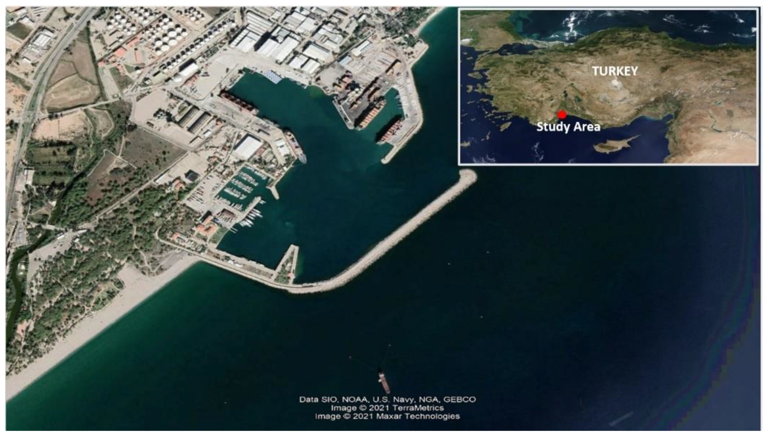
Under the responsibility of the General Command of Mapping of Turkey, sea level monitoring activities in the Turkish coast started in the 1930s. Sea level variations were recorded on daily or weekly charts with an analogous system. Readings were obtained through a float on a cable in a stilling well [23]. The stilling wells were replaced with acoustic gauges later, in 1999 [24,25]. The Turkish National Sea Level Monitoring System (TUDES) had 20 active tide gauge stations along the Turkish coast consisting of a data collection unit with sensors to measure sea level and meteorological factors such as air temperature and air pressure. In this study, hourly sea level and meteorological factors data were derived from the Antalya tide gauge station (see Figure 1) in Antalya Harbor for the period January 2014–December 2015
The sea level and meteorological factors time series gathered at the Antalya tide gauge station are depicted in Figure 2.
The obtained data cover 2-year measurements with 15,000 readings for each parameter. The geodynamic phenomena, such as tectonic motions and land uplift of Earth’s crust, affects the measured sea level height obtained from a tide gauge. Several researchers investigated the geodynamic effects on the Antalya tide gauge station. Yildiz et al. [25] reported that this station showed subsidence with a rate of −5.3 ± 1.8 mm/year based on the GPS observations. Fenoglio-Marc et al. [26] used TOPEX/Poseidon altimetric sea level data to compute the subsidence rate of the same station. The authors found a subsidence rate of −3.0 ± 1.6 mm/year for the study area. More recently, Yildiz et al. [27] estimated the vertical land motion along the southern coast of Turkey, including the Antalya tide gauge station. Both satellite altimetry and GPS data were considered for the estimation. The results showed that the subsidence rate of the station had an average value of 2.93 ± 1.76 mm/year. The vertical land motion of the Earth’s crust was neglected in this study due to a limited time span (2 years) of the obtained data and a low subsidence rate of land motion.
The gaps in the gathered hourly sea level and meteorological factor data were filled with the linear interpolation method as a pre-processing stage of the obtained data. The descriptive statistics such as the mean, maximum, minimum, and standard deviation (SD) of the sea level and meteorological factor data are presented in Table 1.
As shown in Table 1, it was observed that the mean sea level received the highest value in the summer and decreased in the fall, winter, and spring, respectively. The difference between the mean sea level values of winter and summer seasons was measured as 10 cm. In addition, the highest air pressure variations were observed for winter, whereas the lowest ones were observed for summer. For the air temperature, the highest and lowest variations based on the standard deviation were observed in fall and winter. A comparison of the seasonal air pressure and air temperature showed that the relation between them was inversely proportional. For instance, the highest and lowest values of mean air temperature were measured for summer and winter. In contrast, the highest and lowest values of mean air pressure were measured for winter and summer, respectively.
3. Methodology
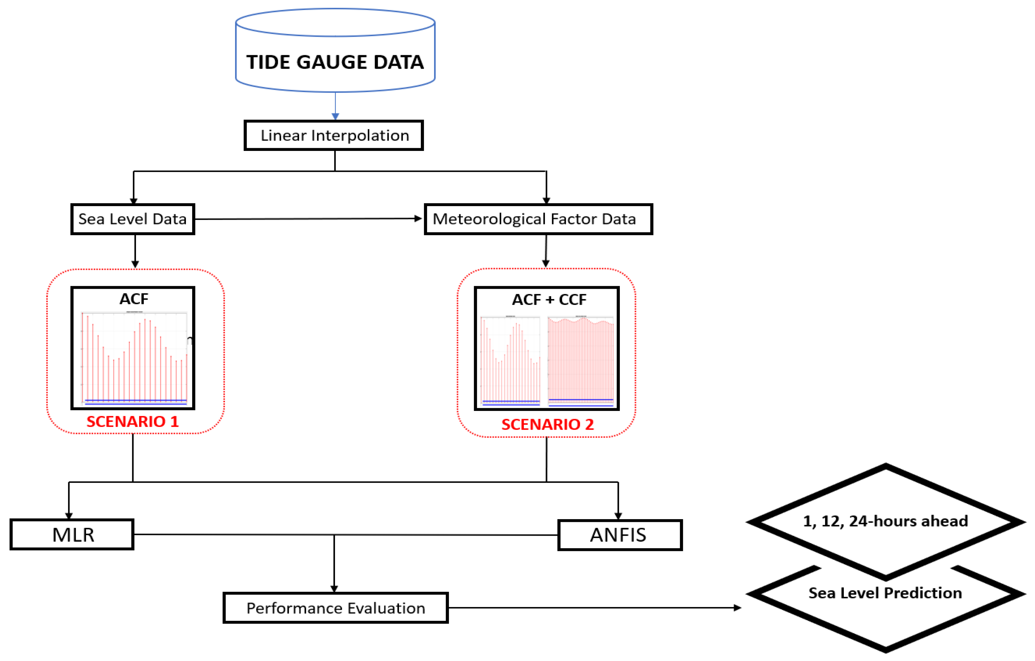
In this study, different MLR and ANFIS models were developed to predict sea level changes based on two different scenarios. The first scenario (SC1) used lagged values of sea level as inputs, and the outputs were the 1, 12, and 24 h ahead of sea level. The second scenario (SC2) used lagged values of both sea level and meteorological factors as inputs, and the outputs are the 1, 12, and 24 h ahead of sea level. The framework for model development consisted of three stages: a pre-processing stage, model development stage, and performance evaluation stage. In the pre-processing stage, a linear interpolation method was used to fill the gaps on the obtained data, and correlation functions such as autocorrelation function (ACF) and cross-correlation functions (CCF) were used to select optimum input selection. In the modelling stages, the dataset was split into training and testing sets according to the Pareto principle, introduced by Macek [28]. To this end, 80% of the data was used as the training data and the remaining 20% was used as testing data sets. Then, several MLR and ANFIS models based on the scenarios and different prediction intervals were developed. Lastly, four different statistical indicators were selected in a multi-objective sense to compare the models’ performance. A flow chart for modelling sea level prediction is presented in Figure 3.
3.1. Multiple Linear Regression
Multiple linear regression (MLR) is a frequently used method of analysis to investigate the linear relation between the inputs and output MLR attempts to model the relationship between one or more independent variable and one dependent variable by fitting a linear equation to the observe data. It can be expressed as:
where y is the predicted (dependent) value, β0 is the y-intercept, βi (i = 1…n) is the regression coefficient of the Xi predictor (independent) value, and ε is the model error. The MLR model can be expressed as the sum of fit and residuals. The best linear fit is determined by considering where the sum of residuals is minimum or equal zero. In Equation (1), β0 and βi are fit terms that represent the best line of fit. The residual can be explained as the difference between the observed and predicted data points.
3.2. Adaptive Neuro-Fuzzy Inference System (ANFIS)
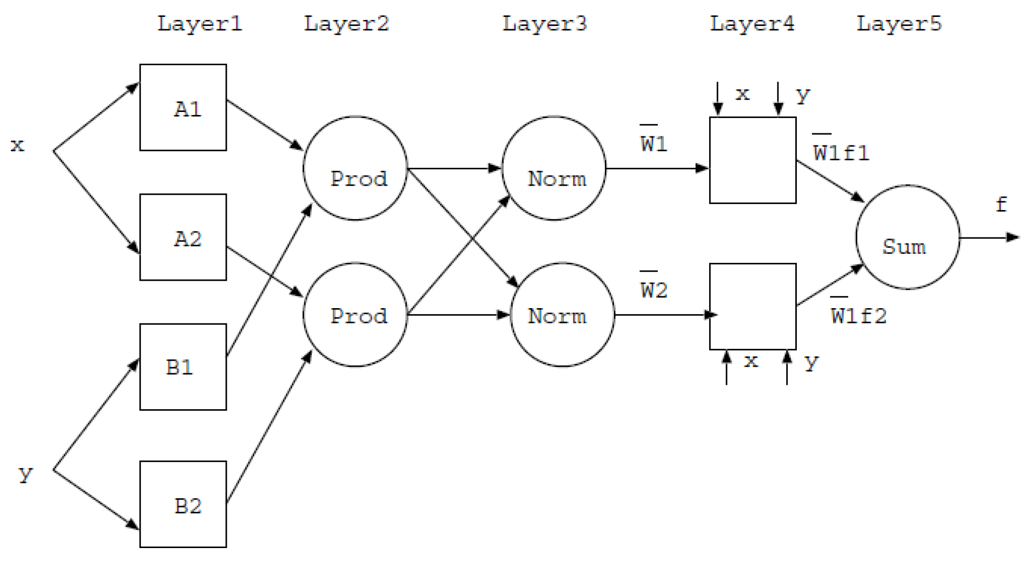
The architecture and learning procedure underlying ANFIS were first presented by Jang [29]. They combine the optimization and learning capabilities of neural networks with fuzzy logic linguistic IF–THEN rules, which consist of membership functions (MF). The first-order Takagi–Sugeno-type ANFIS structure with two inputs and one output can be expressed as follows:
where Ai and Bi (i = 1, 2) are the MF for input x and y. The pi, qi, and ri are the linear parameters and fi is the output function. ANFIS structure is composed of the following five successive layers:
Layer 1: Every node i in this layer is an adaptive node with a node function. Each node gets the values of inputs and membership degrees are calculated.
where O1,i is the output of the ith node, Ai is a linguistic label, and x is the input for node i. Several MF can be chosen, such as a triangular, generalized bell, and gaussian. Each MF produces different membership degrees. A Gaussian membership was chosen in this study and it can be expressed as follows:
where c is the mean and σ is the standard deviation. These parameters are also referred to as “premise parameters”.
Layer 2: The layer is the multiplication of the incoming membership degrees of the successive IF–THEN rules by the logical operation of “and”. The weight or firing strength for the rule is obtained as follows:
Layer 3: The layer calculated weights are normalized by the ratio of each node’s weight to the sum of all nodes’ weight.
The outputs of this layer are called “normalized firing strengths” [21].
Layer 4: The layer where the fractional contribution of each rule in the total output is calculated.
where ϖ is the normalized firing strength from layer 3; pi, qi, and ri are the parameter sets of this node. These are referred to as “consequent parameters” [30].
Layer 5: This is the layer from which the total output was calculated. In this layer, the fuzzy rules are defuzzification and a single value is generated. The output of this layer is named the “overall output”.
The ANFIS structure and layers can be seen in Figure 4. A hybrid learning algorithm can train the ANFIS. The learning process aims to determine the premise parameters (see Layer 1) and consequent parameters (see Layer 4) based on error measures that should be minimized [31]. Error measurement is performed by using the difference between the observed and predicted outputs. RMSE is the source of the ANFIS error measurement process.
3.3. Performance Evaluation
The performance of a prediction model is evaluated by using several statistical indicators. However, there is no agreement on which of them are more reliable for model assessment. Therefore, some researchers [33,34,35,36] indicated that model performance indicators should be selected in a multi-objective sense. According to Ritter and Munoz-Carpena [36], the performance assessment of a model should include at least one absolute value error indicator, one dimensionless indicator for quantifying the goodness of fit, and a graphical representation of the relationship between the model predictions and measurements. To this end, RMSE and MAE were adopted to this study as absolute value error indicators, whereas NSE was adopted as a dimensionless goodness-of-fit indicator. Based on the relevant literature, NSE, and RMSE, MAE, and SI can be defined as below:
where hobserved is the observed value, hpredicted is the predicted value, and N is the sample size.
The NSE value of 1 indicates a perfect match between the observed and predicted values. The NSE value of 0 indicates that the model predictions are accurate for the mean of observed values. However, an NSE value of less than 0 indicates the mean of observed values is more accurate than predictions. An RMSE is evaluated in the range between 0 and 1. An RMSE = 0 indicates the best match between the observed and predicted values.
4. Results and Discussion
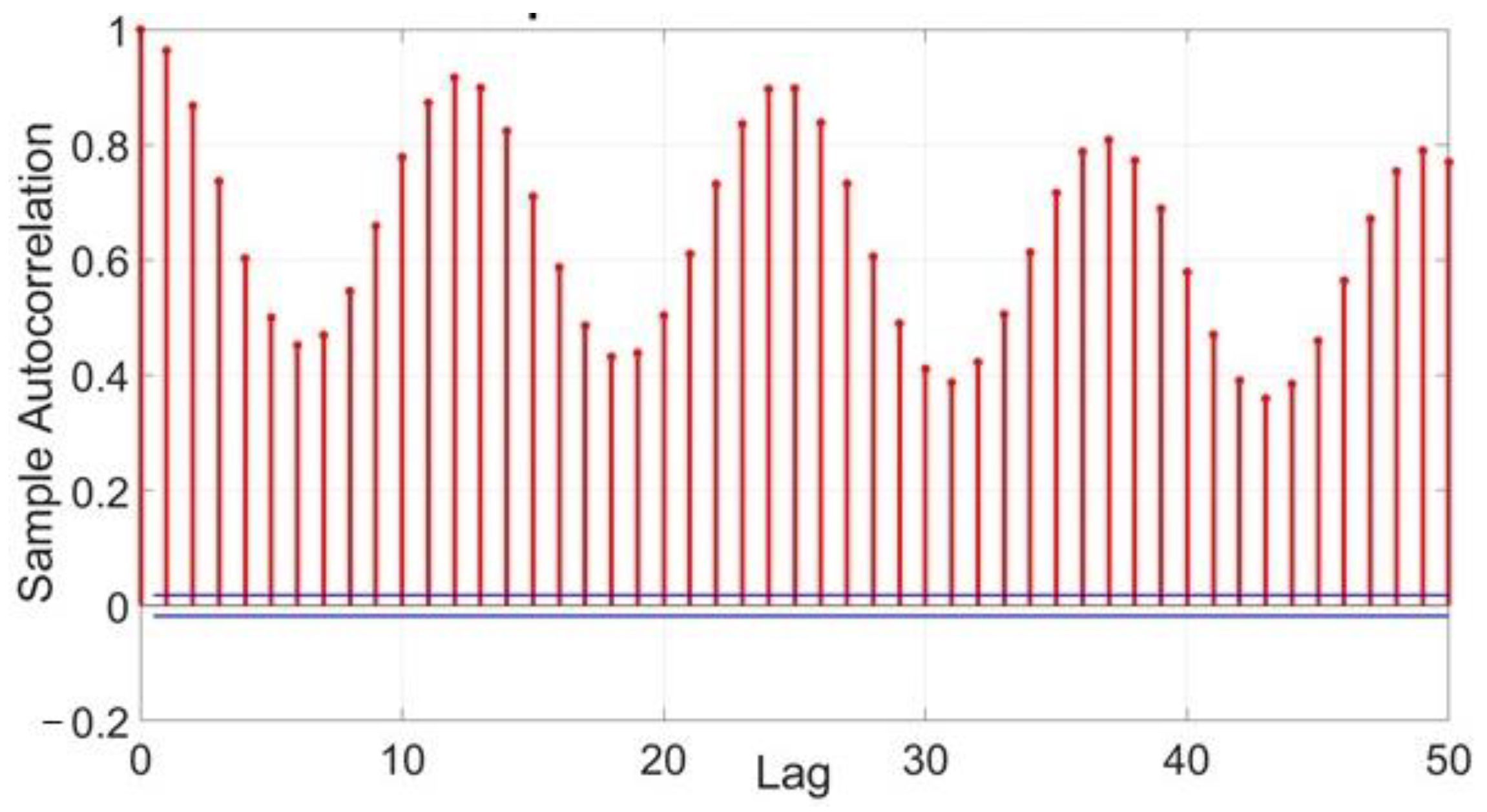
This study collected the hourly sea level and meteorological factor time series (air temperature, air pressure) covering 2 years from the Antalya tide gauge station for sea level prediction. The gaps and missing values on the time series were filled using the linear interpolation method. Based on our literature review, two different scenarios were created that used different input parameters to predict the sea level height 1, 12, and 24 h ahead in Antalya Harbor. The autocorrelation function for the observed sea level time series is presented in Figure 5.
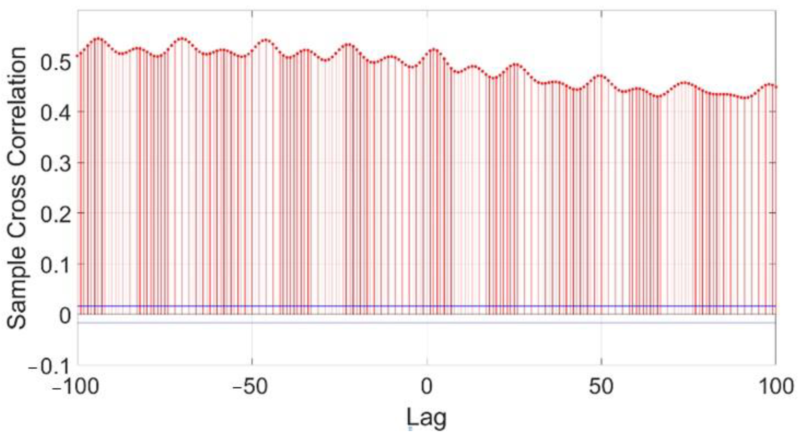
Sea level at time, t, mainly correlated with sea level values at time t-1, t-12, t-13, and t-25. Therefore, these four lagged values of sea level time series were selected as input parameters. The cross-correlation functions for air temperature and air pressure time series are presented in Figure 6 and Figure 7, respectively.
Based on the CCF in Figure 6, it was observed that the correlation between air temperature and sea level time series reached peak values in approximately 24 h periods. The correlation between time series was found as moderate level (R ≅ 0.50). The air temperature was selected as an input parameter for the prediction model.
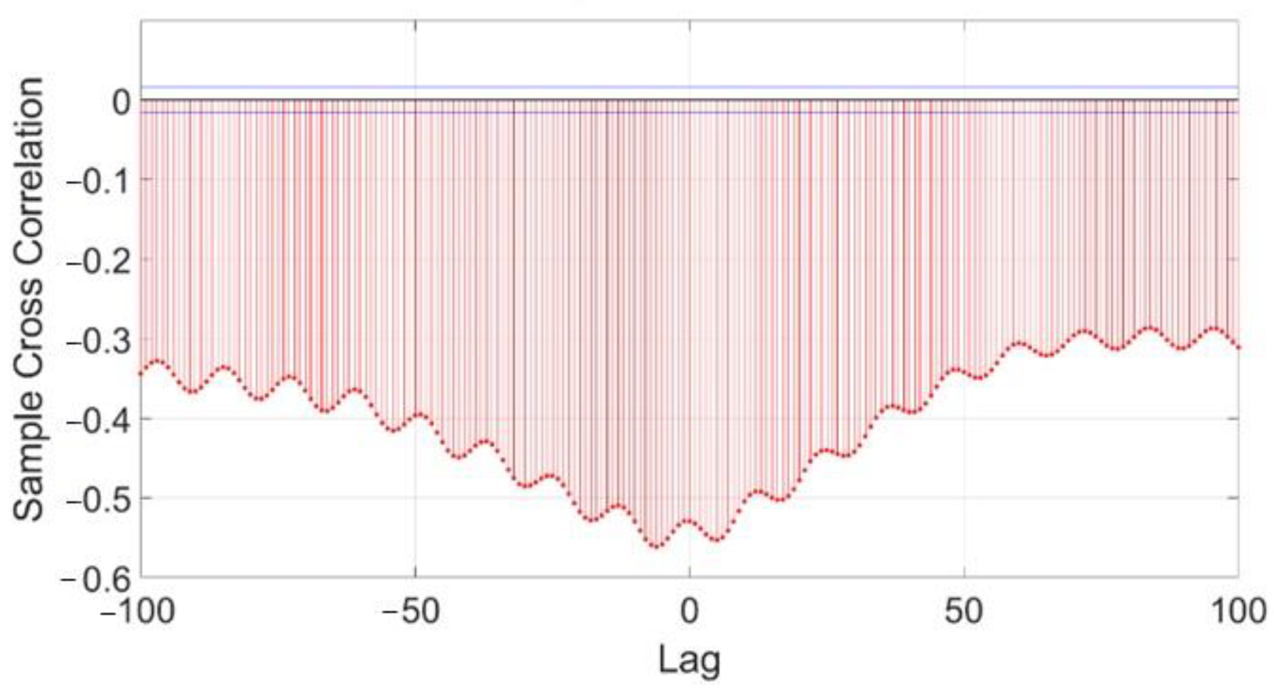
Unlike air temperature, a negative correlation was observed between air pressure and sea level time series (R ≅ −0.55). The best correlation was observed at air pressure values of 5 h (t-5) and 6 h (t-6) time lag. Therefore, lagged air pressure values were selected as input parameters for the prediction model. Two different scenarios were developed which contain the following input and output combinations in a functional form:
where t represents time lag, h represents sea level value, T represents temperature value, and p represents air pressure value.
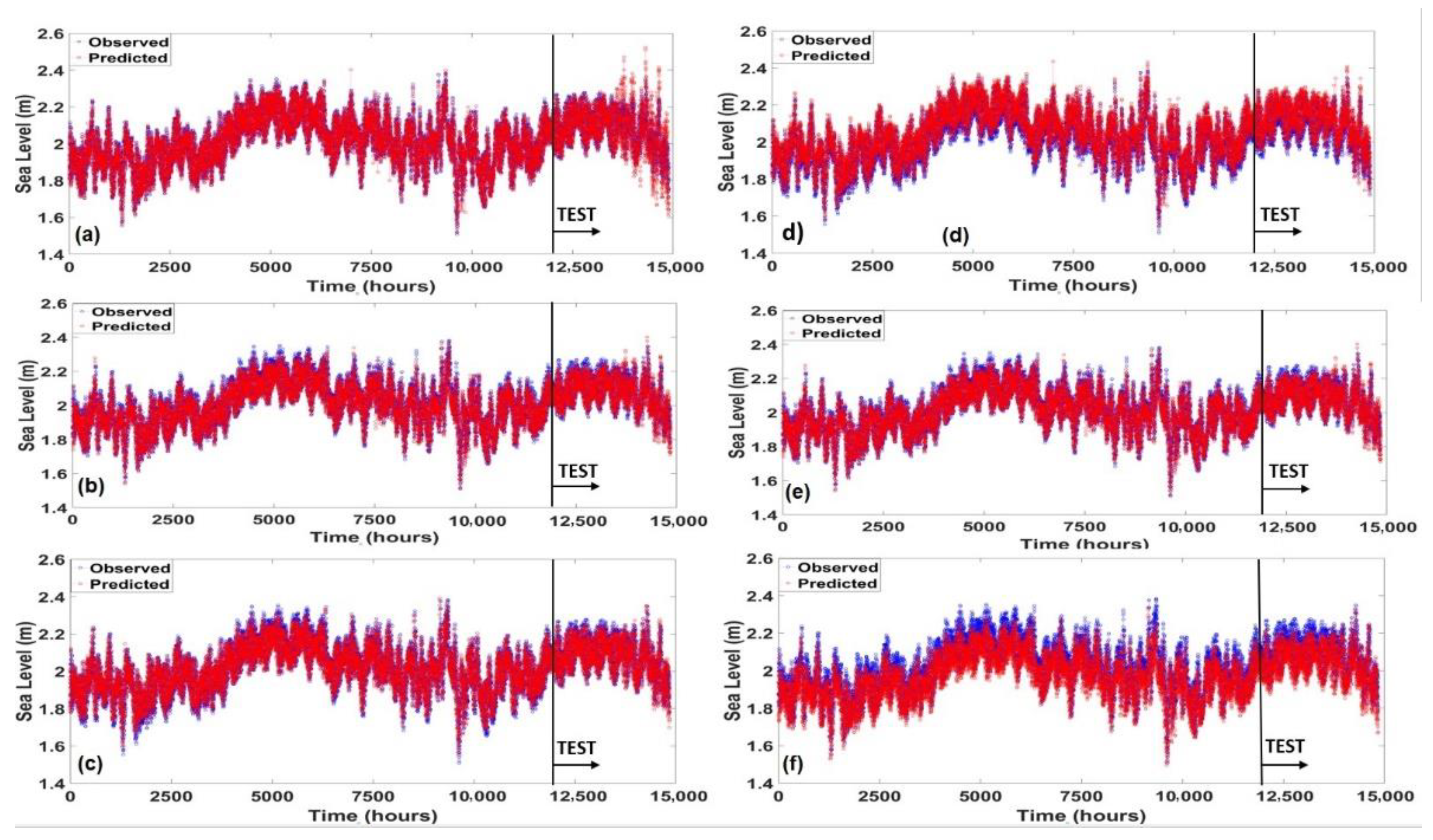
The measured data were divided into train and test sets for all models. A total of 80% of the measured data were used for training and 20% were used for testing. Several MLR and ANFIS models were developed to predict sea level 1, 12, and 24 h ahead using Equations (14) and (15). Focusing on MLR models, regression equations were obtained using trains sets and applied to the test sets to get target sea level values. The simulated sea level time series used MLR model for SC1 and SC2, as presented in Figure 8.
On the other hand, a hybrid learning algorithm was used for the ANFIS model due to its ability to reduce training time. A total of two gaussian membership functions were selected for each input parameter. Although there were several MF types, Vernieuwe et al. [37] reported that the type of MF did not significantly change the results. After 100 epochs, the lowest RMSE values were obtained for the ANFIS model. The simulated sea level time series using the ANFIS model for SC1 and SC2 is presented in Figure 9.
Four statistical indicators mentioned in Section 3.3 were evaluated using Equations (10)–(13) for the MLR and ANFIS models. The statistical performance of the MLR and ANFIS models for SC1 is presented in Table 2. The performance evaluation values were found acceptable for the training stage. Considering the testing stage, the ANFIS model produced the highest test value of NSE, whereas the MLR model produced the lowest test value. The ANFIS model for 1 h-ahead prediction demonstrated an NSE value of more than 0.70 for the model testing stage. It was observed that the ANFIS prediction for 12 h ahead was very near to the MLR prediction for 1 h ahead in terms of NSE. Considering 1-hour-ahead prediction results, it was observed that the performance of the SC1-based ANFIS model produced 32% more accurate results than the SC1-based MLR model. Based on RMSE, MAE, and SI values, the ANFIS models produced lower values than the MLR models for 1-, 12-, and 24 h-ahead predictions. It was observed that the model performance accuracy decreases when the prediction time interval increases. Additionally, the MAE results showed that the SC1-based MLR models can predict the future sea levels with an error range of 4.7 cm to 5.4 cm, whereas the SC1-based ANFIS models can predict with an error range of 2.1 to 5.4 cm. This indicates that the SC1-based ANFIS models are superior to the SC1-based MLR models for sea level prediction.
On the other hand, Figure 8 and Figure 9 indicate that the ANFIS models for predicted sea level followed the observed sea level values better than the MLR model. It was observed that MLR models (especially for Figure 8a,b) produced a longer distance from the observed sea level. This can be interpreted as another sign that ANFIS produces better performance results than MLR.
The statistical performance of the MLR and ANFIS models for SC2 is presented in Table 3. The performance evaluation values were found acceptable for the training stage. Considering the testing stage, the ANFIS model produced the highest test value of NSE, whereas the MLR model produced the lowest test value. Both MLR and ANFIS models for 1 h-ahead prediction demonstrated an NSE value of more than 0.70 for the model testing stage. However, weaker NSE values were evaluated for other models. Surprisingly, it was observed that the SC2-based MLR model for 1 h ahead increases the performance accuracy by 33% compared with the SC1-based MLR models in terms of NSE. However, a comparison of the SC1-based and SC2-based results showed that the increasing prediction intervals decreased the SC2-based model’s accuracy more than the SC1-based model. In contrast to short-term (1 h-ahead) prediction, the contribution of meteorological factors did not improve the model’s performance for increasing prediction intervals. Therefore, the short-term results are in line with the study of El-Diasty and Al-Harbi [4], whereas the longer prediction intervals meteorological effects did not produce a considerable result.
Based on RMSE, MAE, and SI values, the ANFIS models produced lower values than the MLR models for 1-, 12-, and 24 h-ahead predictions. Additionally, the MAE results showed that the SC2-based MLR models can predict future sea levels with an error range of 3.7 cm to 7.1 cm, whereas the SC1-based ANFIS models can predict with an error range of 2.1 to 5.4 cm. Like the SC1-based models, ANFIS can be expressed as the best model for SC2.
From the perspective of modelling performance, the results supported the findings of [9,10,11]. In this study, it can be concluded that ANFIS, a non-linear-based method, is more accurate than the MLR method regardless of the used scenario.
Future sea level prediction is challenging due to the randomness and uncertainty of oceanographic and meteorological conditions. Here, randomness means the non-uniform distribution of sea level and meteorological factors depending on the geographic location. Therefore, sea level prediction studies should be demonstrated considering the case study area. In contrast to the relevant literature reviewed in this study, the Mediterranean coast (southern coast) of Turkey is a closed basin. Therefore, oceanographic, and meteorologic contributions can be less effective for sea level changes when compared with the open-boundary sea locations stated in the reviewed literature, such as the Australian coast [5,6,7,8,11], Singaporean coast [12], Canadian coast [14], Taiwanese coast [15], or Malaysian coast [17,18].
5. Summary and Conclusions
This study aimed to select the best input combinations, compare the linear-based and nonlinear-based models, and present a methodology with a flowchart that can be used for harbor operations for sea level predictions by practitioners. To this end, two different scenarios (SC1 and SC2) with different input combinations were selected. Correlation-based analyses such as ACF and CCF were conducted to reveal optimum input parameters with their lagged times. The CCF results (see Figure 6 and Figure 7) showed that the air temperature had a positive moderate correlation (R ≅ 0.50) with sea level heights. In contrast to air temperature, a negative moderate correlation was found between the air pressure and sea level heights (R ≅ 0.55). Then, several models were developed using MLR and ANFIS methods. The performance of the developed models was evaluated in terms of four statistical indicators. The ANFIS model produced an acceptable performance for SC1, whereas both ANFIS and MLR models produced accurate performance for SC2. Therefore, SC2, which includes meteorological factors such as air temperature and air pressure, can be concluded as the best input combination for sea level prediction for the case study area. The results indicated that adding meteorological factors as input parameters increased the performance accuracy (based on NSE values) of the MLR model up to 33% for short-term sea level predictions. On the other hand, it was observed that ANFIS is superior to MLR for sea level predictions. However, the generalizability of the results is limited by the case study area due to factors that affect sea level changes which differ from region to region.
The influence of oceanographic and meteorological effects was considered in this study. However, the presented methodology can be rearranged using a hydrological process such as rainfall and runoff for further studies.
Author Contributions
Conceptualization, R.T. and E.T.; Formal analysis, R.T. and E.T.; Methodology, R.T., E.T., A.T.H. and A.D.M.; Validation, R.T., E.T., A.T.H. and A.D.M.; Supervision, R.T., A.T.H. and A.D.M.; Validation, R.T., E.T., A.T.H. and A.D.M.; Visualization, R.T. and A.D.M.; Writing—original draft, R.T., E.T.; Writing—review & editing, R.T., A.T.H. and A.D.M. All authors have read and agreed to the published version of the manuscript.
Funding
This research was supported by the Maa- ja vesitekniikan tuki r.y. (MVTT) with the project number 41878.
Institutional Review Board Statement
Not applicable.
Informed Consent Statement
Not applicable.
Data Availability Statement
The data supporting the findings of this paper is available from corresponding author upon reasonable request.
Acknowledgments
This work was supported by the Maa- ja vesitekniikan tuki r.y. (MVTT) with the project number 41878, to which the authors would like to express their deep gratitude.
Conflicts of Interest
The authors declare no conflict of interest.
References
- Mimura, N. Sea level rise caused by climate change and its implications for society. Proc. Jpn. Acad. Ser. B 2013, 89, 281–301. [Google Scholar] [CrossRef] [Green Version]
- IPCC. Climate Change 2007—The Physical Science Basis: Contribution of Working Group I to the Fourth Assessment Report of the IPCC; Solomon, S., Qin, D., Manning, M., Chen, Z., Marquis, M., Averyt, K.B., Tignor, M., Miller, H.L., Eds.; Cambridge University Press: Cambridge, UK, 2007.
- Cazaneva, A.; Nerem, R.S. Present-day sea level change: Observations and causes. Rev. Geophys. 2004, 42, 1–20. [Google Scholar] [CrossRef]
- El-Diasty, M.; Al-Harbi, S. Development of wavelet network model for accurate water levels prediction with meteorological effects. Appl. Ocean Res. 2015, 53, 228–235. [Google Scholar] [CrossRef]
- Makarynska, D.; Makarynskyy, O. Predicting sea-level variations at the Cocos (Keeling) Islands with artificial neural networks. Comput. Geosci. 2008, 34, 1910–1917. [Google Scholar] [CrossRef]
- Makarynskyy, O.; Makarynska, D.; Kuhn, M.; Featherstone, W.E. Predicting sea level variations with artificial neural networks at Hillary Boat Harbor, Western Australia. Estuar. Coast. Shelf Sci. 2004, 61, 351–360. [Google Scholar] [CrossRef] [Green Version]
- Ghorbani, M.A.; Makarynskyy, O.; Shiri, J.; Makarynska, D. Genetic programming for sea level predictions in an island environment. Int. J. Ocean Clim. Syst. 2010, 1, 27–35. [Google Scholar] [CrossRef]
- Ghorbani, M.A.; Khatibi, R.; Aytek, A.; Makarynskyy, O.; Shiri, J. Sea water level forecasting using genetic programming and comparing the performance with the artificial neural networks. Comput. Gesci. 2010, 36, 620–627. [Google Scholar] [CrossRef]
- Pashova, L.; Popova, S. Daily Sea level forecast at tide gauge Burgas, Bulgaria using artificial neural networks. J. Sea Res. 2011, 66, 154–161. [Google Scholar] [CrossRef]
- Shiri, J.; Makarynskyy, O.; Kisi, O.; Dierickx, W.; Fard, A. Prediction of short-term operational water levels using an adaptive neuro-fuzzy inference system. J. Waterw. PortCoast. Ocean Eng. 2011, 137, 344–354. [Google Scholar] [CrossRef]
- Karimi, S.; Kisi, O.; Shiri, J.; Makarnyskyy, O. Neuro-fuzzy and neural-network techniques for forecasting sea level in Darwin Harbor, Australia. Comput. Geosci. 2013, 52, 50–59. [Google Scholar] [CrossRef]
- Kurniawan, A.; Ooi, S.K.; Babovic, V. Improved Sea level anomaly prediction through combination of the data relationship and genetic programming in Singapore regional waters. Comput. Geosci. 2014, 72, 94–104. [Google Scholar] [CrossRef]
- Kaloop, M.R.; Rabah, M.; Elnabwy, M. Sea level change analysis and models identification based on short tidal gauge measurements in Alexandria, Egypt. Mar. Geod. 2016, 39, 1–20. [Google Scholar] [CrossRef]
- Kaloop, M.R.; El-Diasty, M.; Wan Hu, J. Real-time prediction of water level change using adaptive neuro-fuzzy inference system. Geomat. Nat. HazardsRisk 2017, 8, 1320–1332. [Google Scholar] [CrossRef]
- Imani, M.; Huan-Chin, K.; Wen-Hau, L.; Chung-Yen, K. Daily Sea level prediction at Chiayi coast, Taiwan using extreme learning machine and relevance learning machine. Glob. Planet. Chang. 2018, 161, 211–221. [Google Scholar] [CrossRef]
- Altunkaynak, A.; Kartal, E. Performance comparison of continuous wavelet-fuzzy and discrete wavelet-fuzzy models for water level predictions at the northern and southern boundary of Bosphorus. Ocean Eng. 2019, 186, 106097. [Google Scholar] [CrossRef]
- Lai, V.; Ahmed, A.N.; Malek, M.A.; Abdulmohsin Afan, H.; Ibrahim, R.K.; El-Shafie, A.; El-Shafie, A. Modelling the nonlinearity of sea level oscillations in the Malaysian coastal areas using machine learning algorithms. Sustainability 2019, 11, 4643. [Google Scholar] [CrossRef] [Green Version]
- Muslim, T.O.; Ahmed, A.N.; Malek, M.A.; Abdulmohsin Afan, H.; Ibrahim, R.K.; El-Shafie, A.; Sapitang, M.; Sherif, M.; Sefelnasr, A.; El-Shafie, A. Investigating the influence of meteorological parameters on the accuracy of sea-level prediction models in Sabah, Malaysia. Sustainability 2020, 12, 1193. [Google Scholar] [CrossRef] [Green Version]
- Altunkaynak, A.; Kartal, E. Transfer Sea level learning in the Bosphorus Strait by wavelet-based machine learning methods. Ocean Eng. 2021, 233, 109116. [Google Scholar] [CrossRef]
- Song, C.; Chen, X.; Ding, X.; Zhang, L. Sea level simulation with signal decomposition and machine learning. Ocean Eng. 2021, 241, 110109. [Google Scholar] [CrossRef]
- Di Nunno, F.; de Marinis, G.; Gargano, R.; Granata, F. Tide prediction in the Venice Lagoon using nonlinear autoregressive exogenous (NARX) neural network. Water 2021, 13, 1173. [Google Scholar] [CrossRef]
- Granata, F.; Di Nunno, F. Artificial intelligence models for prediction of the tide level in Venice. Stoch. Environ. Res. Risk Assess. 2021, 35, 2537–2548. [Google Scholar] [CrossRef]
- Seseogullari, B.; Eris, E.; Kahya, E. Trend analysis of sea levels along the Turkish Coast. Hydrol. Days 2007, 19–21, 152–160. [Google Scholar]
- Simav, M.; Yildiz, H.; Turkezer, A.; Lenk, O.; Ozsoy, E. Sea level variability at Antalya and Menteş tide gauges in Turkey: Atmospheric, steric, and land motion contributions. Studia Geophys. Geod. 2012, 56, 215–230. [Google Scholar] [CrossRef]
- Yildiz, H.; Demir, C.; Gürdal, M.A.; Akabalı, O.A.; Demirkol, E.O.; Ayhan, M.E.; Turkoglu, Y. Antalya-II, Bodrum-II, Erdek ve Menteş mareograf istastonlarına ait 1984–2002 yılları arası deniz seviyesi ve jeodezik ölçülerin değerlendirilmesi. Harita Dergi 2003, 17, 5–72. [Google Scholar]
- Fenoglio-Marc, L.; Braitenberg, C.; Tunini, L. Sea level variability and trends in the Adriatic Sea in 1993–2008 from tide gauges and satellite altimetry. Phys. Chem. Earth 2012, 40, 47–58. [Google Scholar] [CrossRef]
- Yidiz, H.; Andersen, O.B.; Simav, M.; Aktug, B.; Ozdemir, S. Estimates of the vertical land motion along the southwestern coasts of Turkey from coastal altimetry and tide gauge data. Adv. Space Res. 2013, 51, 1572–1580. [Google Scholar] [CrossRef]
- Macek, K. The pareto principle in datamining: An above-average fencing algorithm. Acta Polytech 2008, 48, 55–59. [Google Scholar] [CrossRef]
- Jang, J.S.R. Adaptive-network based fuzzy inference system. IEEE Trans. Syst. ManCybern. 1993, 23, 665–685. [Google Scholar] [CrossRef]
- Mathworks. MATLAB Fuzzy Toolbox User’s Guide; The MathWorks: Natick, MA, USA, 2018. [Google Scholar]
- Yildirim, G.; Ozger, M. Neuro-fuzzy approach in estimating Hazen-Williams friction coefficient for small-diameter polyethylene pipes. Adv. Eng. Softw. 2009, 40, 593–599. [Google Scholar] [CrossRef]
- Tur, R.; Balas, C.E. Neuro-fuzzy approximation for prediction of significant wave heights: The case of Filyos region. J. Fac. Eng. Archit. Gazi Univ. 2010, 25, 505–510. [Google Scholar]
- Legates, D.R.; McCabe, G.J. Evaluating the use of “goodness-of-fit” measures in hydrologic and hydro-climatologic model variation. Water Resour. Res. 1999, 35, 233–241. [Google Scholar] [CrossRef]
- Karimi, B.; Safari, M.; Mehr, A.D.; Mohammadi, M. Monthly rainfall prediction using ARIMA and gene expression programming: A case study in Urmia, Iran. Online J. Eng. Sci. Technol. 2019, 2, 8–14. [Google Scholar]
- Mehr, A.D.; Gandomi, A.H. MSGP-LASSO: An improved multi-stage genetic programming model for streamflow prediction. Inf. Sci. 2021, 561, 181–195. [Google Scholar] [CrossRef]
- Ritter, A.; Munoz-Carpena, R. Performance evaluation of hydrological models: Statistical significance for reducing subjectivity in goodness-of-fit assessment. J. Hydrol. 2013, 480, 33–45. [Google Scholar] [CrossRef]
- Vernieuwe, H.; Geogieva, O.; De Baets, B.; Pauewels, V.R.N.; Verhoest, N.E.C.; De Troch, F.P. Comparison of data-driven takani-sugeno models of rainfall-discharge dynamics. J. Hydrol. 2005, 302, 173–186. [Google Scholar] [CrossRef]
Figure 1.
Location of the study area.

Figure 2.
Time series of (a) sea level; (b) air temperature; (c) air pressure observed at Antalya tide gauge station.
Figure 2.
Time series of (a) sea level; (b) air temperature; (c) air pressure observed at Antalya tide gauge station.

Figure 3.
Flow chart for sea level prediction methodology.

Figure 4.
Adaptive neuro-fuzzy inference system (ANFIS) structure (after [32]).
Figure 4.
Adaptive neuro-fuzzy inference system (ANFIS) structure (after [32]).

Figure 5.
The autocorrelation function for sea level time series.

Figure 6.
The cross-correlation functions between air temperature and sea level time series.

Figure 7.
The cross-correlation functions between air pressure and sea level time series.

Figure 8.
Multiple linear regression predictions: (a) SC1-based 1 h ahead; (b) SC1-based 12 h ahead; (c) SC1-based 24 h ahead; (d) SC2-based 1 h ahead; (e) SC2-based 12 h ahead; (f) SC2-based 24 h ahead.
Figure 8.
Multiple linear regression predictions: (a) SC1-based 1 h ahead; (b) SC1-based 12 h ahead; (c) SC1-based 24 h ahead; (d) SC2-based 1 h ahead; (e) SC2-based 12 h ahead; (f) SC2-based 24 h ahead.

Figure 9.
Adaptive neuro-fuzzy inference system predictions: (a) SC1-based 1 h ahead; (b) SC1-based 12 h ahead; (c) SC1-based 24 h ahead; (d) SC2-based 1 h ahead; (e) SC2-based 12 h ahead; (f) SC2-based 24 h ahead.
Figure 9.
Adaptive neuro-fuzzy inference system predictions: (a) SC1-based 1 h ahead; (b) SC1-based 12 h ahead; (c) SC1-based 24 h ahead; (d) SC2-based 1 h ahead; (e) SC2-based 12 h ahead; (f) SC2-based 24 h ahead.


Table 1.
Descriptive statistics of observed data.
| Parameters | Statistics | Entire | Fall | Winter | Spring | Summer |
|---|---|---|---|---|---|---|
| SEA LEVEL (m) | Mean | 2.02 | 2.05 | 1.99 | 1.97 | 2.09 |
| Maximum | 2.56 | 2.37 | 2.56 | 2.43 | 2.41 | |
| Minimum | 1.49 | 1.68 | 1.49 | 1.54 | 1.77 | |
| SD | 0.13 | 0.10 | 0.14 | 0.11 | 0.10 | |
| TEMPERATURE (°C) | Mean | 20.13 | 21.88 | 12.01 | 17.69 | 28.24 |
| Maximum | 42.73 | 37.87 | 22.76 | 33.56 | 42.73 | |
| Minimum | −1.53 | 6.73 | −1.53 | −0.20 | 16.08 | |
| SD | 7.20 | 4.96 | 3.37 | 4.11 | 3.52 | |
| PRESSURE (mb) | Mean | 988.78 | 987.72 | 1001.04 | 989.19 | 977.01 |
| Maximum | 1018.90 | 1029.80 | 1032.90 | 1029.90 | 1017.00 | |
| Minimum | 918.32 | 925.63 | 918.32 | 927.29 | 923.87 | |
| SD | 28.88 | 30.54 | 22.19 | 26.12 | 30.70 |
Table 2.
Statistical performance of the SC1-based MLR and ANFIS models.
| Intervals | MLR TRAIN | MLR TEST | ANFIS TRAIN | ANFIS TEST | ||||||||||||
|---|---|---|---|---|---|---|---|---|---|---|---|---|---|---|---|---|
| NSE | RMSE (m) | MAE (m) | SI | NSE | RMSE (m) | MAE (m) | SI | NSE | RMSE (m) | MAE (m) | SI | NSE | RMSE (m) | MAE (m) | SI | |
| (t + 1) | 0.98 | 0.018 | 0.012 | 0.009 | 0.59 | 0.074 | 0.047 | 0.036 | 0.98 | 0.017 | 0.012 | 0.008 | 0.88 | 0.040 | 0.021 | 0.020 |
| (t + 12) | 0.88 | 0.045 | 0.031 | 0.022 | 0.45 | 0.084 | 0.047 | 0.040 | 0.89 | 0.043 | 0.030 | 0.021 | 0.53 | 0.077 | 0.043 | 0.037 |
| (t + 24) | 0.82 | 0.056 | 0.040 | 0.028 | 0.30 | 0.093 | 0.054 | 0.045 | 0.83 | 0.054 | 0.039 | 0.027 | 0.36 | 0.089 | 0.054 | 0.043 |
Table 3.
Statistical performance of the SC2-based MLR, ANFIS models.
| Intervals | MLR TRAIN | MLR TEST | ANFIS TRAIN | ANFIS TEST | ||||||||||||
|---|---|---|---|---|---|---|---|---|---|---|---|---|---|---|---|---|
| NSE | RMSE (m) | MAE (m) | SI | NSE | RMSE (m) | MAE (m) | SI | NSE | RMSE (m) | MAE (m) | SI | NSE | RMSE (m) | MAE (m) | SI | |
| (t + 1) | 0.93 | 0.034 | 0.030 | 0.017 | 0.79 | 0.053 | 0.037 | 0.025 | 0.98 | 0.017 | 0.012 | 0.008 | 0.88 | 0.040 | 0.021 | 0.020 |
| (t + 12) | 0.88 | 0.046 | 0.033 | 0.023 | 0.45 | 0.083 | 0.048 | 0.040 | 0.89 | 0.043 | 0.030 | 0.021 | 0.44 | 0.085 | 0.047 | 0.041 |
| (t + 24) | 0.70 | 0.072 | 0.058 | 0.035 | 0.08 | 0.107 | 0.071 | 0.05 | 0.84 | 0.053 | 0.038 | 0.026 | 0.25 | 0.097 | 0.054 | 0.047 |
Publisher’s Note: MDPI stays neutral with regard to jurisdictional claims in published maps and institutional affiliations. |
© 2021 by the authors. Licensee MDPI, Basel, Switzerland. This article is an open access article distributed under the terms and conditions of the Creative Commons Attribution (CC BY) license (https://creativecommons.org/licenses/by/4.0/).
Share and Cite
MDPI and ACS Style
Tur, R.; Tas, E.; Haghighi, A.T.; Mehr, A.D. Sea Level Prediction Using Machine Learning. Water 2021, 13, 3566. https://doi.org/10.3390/w13243566
AMA Style
Tur R, Tas E, Haghighi AT, Mehr AD. Sea Level Prediction Using Machine Learning. Water. 2021; 13(24):3566. https://doi.org/10.3390/w13243566
Chicago/Turabian StyleTur, Rifat, Erkin Tas, Ali Torabi Haghighi, and Ali Danandeh Mehr. 2021. "Sea Level Prediction Using Machine Learning" Water 13, no. 24: 3566. https://doi.org/10.3390/w13243566
Note that from the first issue of 2016, this journal uses article numbers instead of page numbers. See further details here.