
Vortex Dynamics Analysis of Internal Flow Field of Mixed-Flow Pump under Alford Effect


1
National Research Center of Pumps, Jiangsu University, Zhenjiang 212013, China
2
Institute of Fluid Engineering Equipment Technology, Jiangsu University, Zhenjiang 212009, China
3
College of Mechanical Engineering, Nantong University, Nantong 226019, China
4
Department of Mechanical Engineering & Materials Science, Washington University in St. Louis, St. Louis, MO 63130, USA
*
Authors to whom correspondence should be addressed.
Water 2021, 13(24), 3575; https://doi.org/10.3390/w13243575
Submission received: 21 October 2021
/
Revised: 1 December 2021
/
Accepted: 3 December 2021
/
Published: 13 December 2021
(This article belongs to the Special Issue CFD in Fluid Machinery Design and Optimization)
Abstract
:A multi-region dynamic slip method was established to study the internal flow characteristics of the mixed-flow pump under the Alford effect. The ANSYS Fluent software and the standard k-ε two-equation model were used to numerically predict the mixed-flow pump’s external characteristics and analyze the forces on the impeller and guide vane internal vortex structure and non-uniform tip gap of the mixed-flow pump at different eccentric distances. The research results show that the external characteristic results of the numerical calculation are consistent with the experimental measurement. The head error of the design flow operating point is about 5%, and the efficiency error is no more than 3%, indicating the high accuracy of numerical calculation. Eccentricity has a significant influence on the flow field in the tip area of the mixed-flow pump impeller, the distribution of vortex core in the impeller presents obvious asymmetry, the strength and distribution area of the vortex core in the small gap area of the tip increase obviously, which aggravates the flow instability and increases the energy loss. With the increase of eccentricity, the strength and number of vortex core structures in the guide vane also increase significantly, and obvious flow separation occurs near the inlet of the guide vane suction surface on the eccentric side of the impeller. The circumferential distribution of L1 and L2 values represents the friction pressure gap in the eccentric state, and the eccentricity has a more noticeable effect on L1 and L2 values at the small gap; With the increase of eccentricity, the values of vorticity moment components L1 and L2 increase, and the Alford moment on the impeller increases. The leading-edge region of the blade is the main part affected by the unstable torque of the flow field. With the increase of eccentricity, the impact degree of tip leakage flow deepens, and the change of the tip surface pressure is the most obvious. The impact area of tip leakage flow is mainly concentrated in the first half of the impeller channel, which has an impact on the blade inlet flow field but has little impact on the blade outlet flow field.
1. Introduction
The Alford effect is the rotor dynamics effect caused by the fluid flow in the gap area between the blade tip and the stationary shell of the turbo-machinery. This effect is due to the irregular force on the blade and the eccentric operation of the impeller, which produces a diagonal fluid excitation force and acts on the impeller, thus aggravating the whirl of the rotor subsystem [1,2,3,4]. As a typical hydraulic machine, the mixed-flow pump inevitably has mass eccentricity [5] due to poor quality control, manufacturing error, assembly error, uneven material, and other reasons during the processing of rotor parts, which leads to the Alford effect and induces rotor vibration instability. Therefore, it is of great significance to study the hydraulic characteristics of mixed-flow pumps under the Alford effect and explore the essence of the vortex flow field of mixed-flow pumps.
At present, some achievements have been made in the research of the eccentricity of rotating machinery. Brennen [6] theoretically analyzed the generation mechanism of an exciting fluid force in the blade tip clearance of an axial-flow pump, gave the theoretical calculation formula of Alford force, and discussed the influence of vortex direction on Alford force. With the rapid development of computer technology, in the field of pump research, CFD calculation gradually replaces real machine tests to simulate the pump’s external characteristics and internal flow field, which significantly reduces the product test and production cycle of the pump and reduces the processing cost. Moore [7] established a three-dimensional calculation model of an eccentric impeller of centrifugal water pump using three-dimensional CFD technology and analyzed the excitation force of a zero static eccentric vortex rotor shroud and mainstream under different precision frequency ratios. Shinichiro [8] experimentally studied the fluid force during eccentric rotation of the centrifugal impeller under different tip clearance, measured the unsteady pressure in the end wall area, and analyzed the internal flow field of the pump based on CFD. Li Wei [9], based on RNG k-ε, designed a model that simulates the internal flow field of the mixed-flow pump under the eccentricity of 0 mm, 0.3 mm, and 0.5 mm, and revealed the flow characteristics of the non-uniform tip clearance flow field of the mixed-flow pump. Shoji [10] and Adkins [11] respectively analyzed the fluid excitation force in the centrifugal impeller vortex by using the potential flow theory and pure dynamics models. The research shows that the fluid excitation force acting on the impeller outlet is dominant when the vortex rate is relatively low and studied the vortex of the open centrifugal impeller. However, the above documents judge the quality of the flow field through the pressure distribution of the conventional flow field [12,13,14,15], which cannot fully reveal the generation and development of vorticity in the eddy flow field and its interaction mechanism with the object wall. Chuochua [16] solved the three-dimensional transient flow in the seal clearance during whirling by using a dynamic grid and unsteady method and extracted the frequency-related rotor dynamic characteristic coefficient. Zhang Liang et al. [17] applied the vortex dynamics theory to the study of the internal flow of Francis turbine runners. They predicted the flow separation on the blade suction surface under low flow conditions according to its internal vortex core distribution. Li Fengchao [18] introduced the theory of boundary vorticity dynamics to simulate the whole channel three-dimensional turbulence of guide vane and blade profile, analyzed the distribution state of boundary vorticity flow on the surface of guide vane and blade, and found the parts with poor local flow. Xu Zhaohui [19] used the BVF method to diagnose the surface flow field of high-speed centrifugal pump blades and captured the drastic changes of BVF at the corresponding positions where cracks appear. Fan Honggang et al. [20,21] carried out BVF analysis on the surface flow field of the reversible runner by using the eddy dynamics method, which provides a diagnostic basis for runner design. However, up to now, the vortex dynamics research on the internal flow field of mixed-flow pumps under the Alford effect has not been reported publicly. Especially under the Alford effect, due to the vortex of the impeller, it is not suitable to divide the calculation domain of the impeller section by using the static grid. Although the moving grid method can effectively solve the problem of boundary movement with time, the technology is not mature enough to effectively simulate the internal flow field structure under impeller whirl [22,23,24,25]. Therefore, it is necessary to explore a new model to calculate the impeller vortex under the Alford effect.
Taking the mixed-flow pump as the research object, based on the previous study of its internal flow and shafting vibration [26,27,28,29], the numerical calculation method of a mixed-flow pump under the Alford effect is established, and the vortex structure of non-uniform blade tip clearance is identified by using the Q-criterion method. Based on the vorticity moment theorem, the stress of non-uniform blade tip clearance is analyzed, and the internal flow of the mixed-flow pump under the Alford effect is explored.
2. Simulation Model
2.1. 3D Solid Modeling
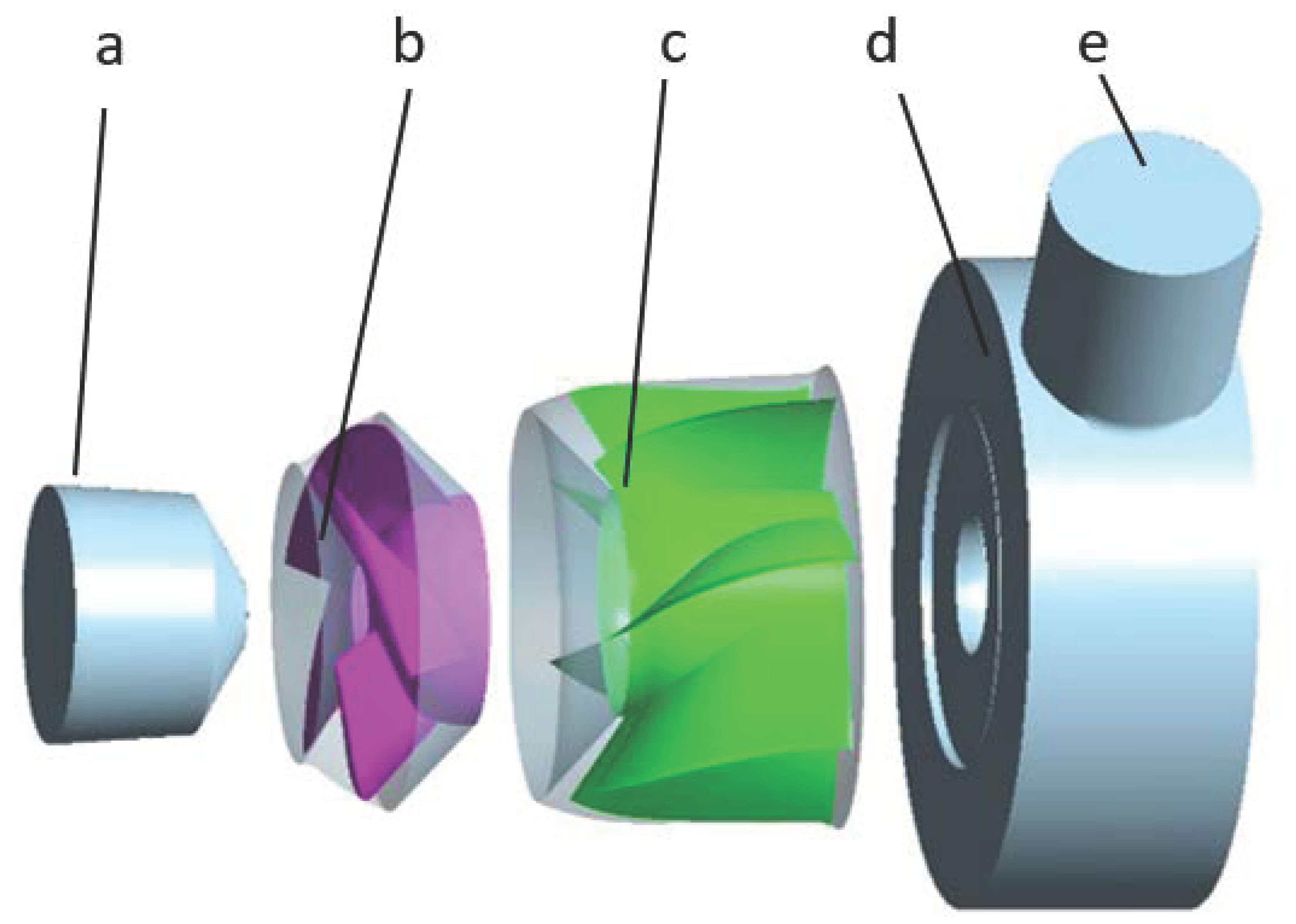
The research model is a guide vane mixed-flow pump. The design parameters are flow Q = 380 m3/h, head H = 6 m, rotating speed n = 1450 r/min, specific speed ns = 480, number of blades Z = 4, and number of guide vanes Zd = 7. The inlet diameter of the pump is 250 mm, the outlet diameter is 200 mm, and the blade top clearance is 0.8 mm. Pro/E software is used to model the inlet section, impeller, guide vane, volute chamber, and outlet section of the model, respectively. After assembly, the three-dimensional solid modeling of the whole flow channel of the mixed-flow pump is obtained. The calculation area is the whole device section from the inlet section of the pump to the outlet section of the annular volute chamber, as shown in Figure 1.
2.2. Impeller Vortex Model
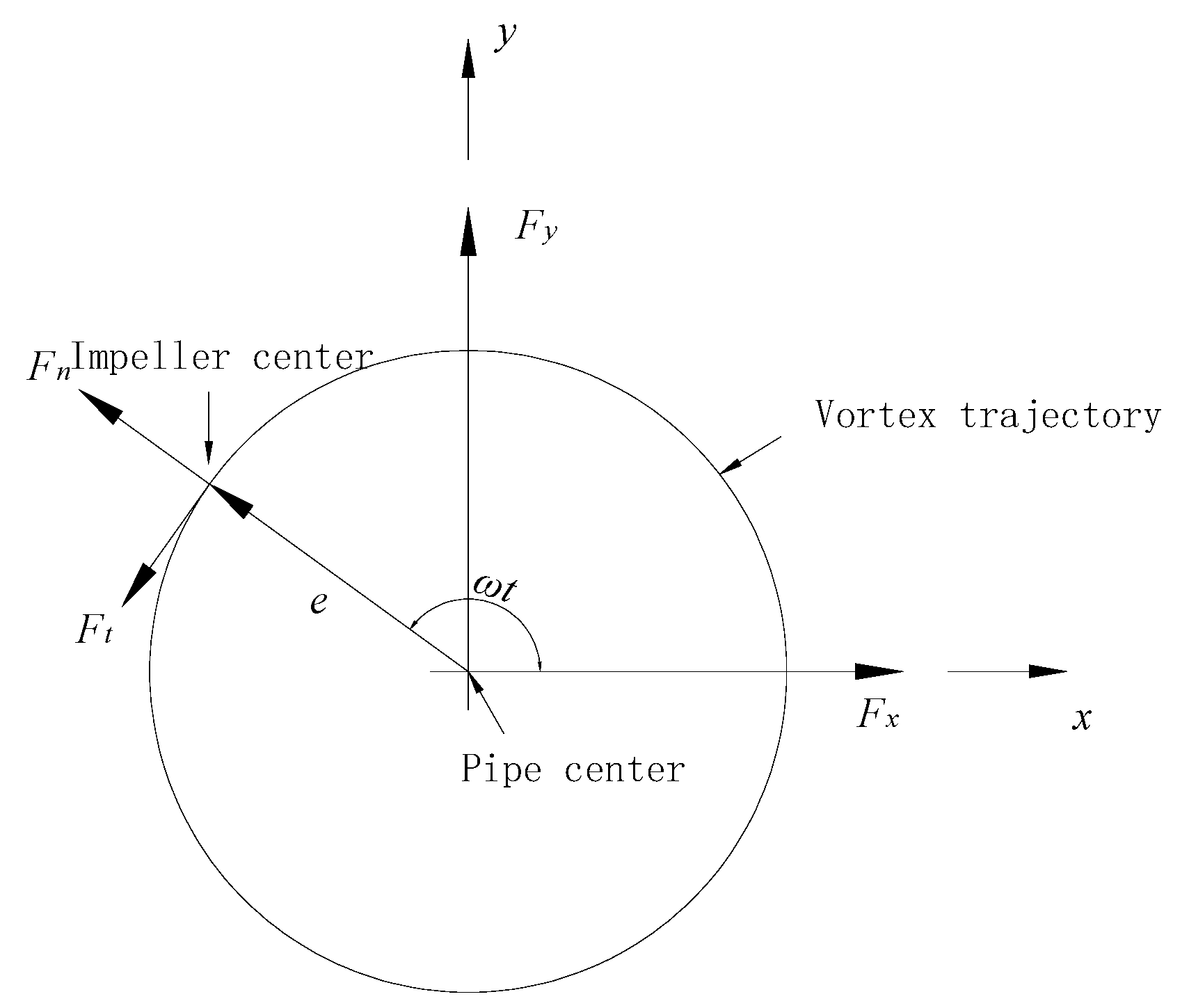
Under the Alford effect, there is an eccentricity between the central axis of the mixed-flow pump impeller and the central axis of the runner chamber. Therefore, there will be forward or reverse whirl (or precession) rotation in the process of rotation while the impeller rotates [30]. Therefore, when simulating the flow field, considering that the impeller has rotation and whirl, it is necessary to introduce the impeller whirl model [31], as shown in Figure 2, where e is the eccentricity; in this paper, the eccentricity of the mixed-flow pump impeller is 0 mm, 0.3 mm, and 0.5 mm, respectively.
In the vortex model, the resultant external force acting on the rotating impeller can be decomposed into standard component Fn and tangential component Ft. When solving, the standard component Fn and tangential component Ft are usually used as the vortex frequency ratio ω/n The dimensionless form of the function of n is as follows:
where M, m, c, C, K, and k are eddy characteristic coefficients used to analyze the influence of fluid force inside the impeller on rotor dynamic characteristics [32]. M is the directly added mass coefficient; m is the added mass coefficient of cross-coupling; C is the direct damping coefficient; c is the cross-coupling damping coefficient; K is the direct stiffness coefficient; k is the cross-coupling stiffness coefficient. To simplify the research, the vortex frequency ratio of the mixed-flow pump impeller is (ω/n) set to 0, 0.2, 0.4, 0.6, 0.8, and 1.0, respectively.
3. Dynamic Sliding Multi-Region Method
3.1. Governing Equation and Turbulence Model
At present, in the numerical calculation of mixed-flow pumps, the standard k-ε two-equation model is widely used in engineering, and its numerical prediction results match well with the test results [33,34]. The k-ε model with the enhanced wall treatment option activated is suitable for jet impact calculation, rotating flow, high-pressure gradient, and recirculation flow. Therefore, this turbulence model is used to study the unsteady flow characteristics in mixed-flow pumps under the Alford effect [35]. Standard k-ε is the close of Reynolds time-averaged N-S equation. The two-equation model introduces an equation about the turbulent energy dissipation rate, continuity equation, and momentum equation to form a control equation group. Assuming that the fluid is incompressible, in standard k-ε in the two-equation model, turbulent kinetic energy k, and dissipation rate ε, the constraint equation is
The expression of turbulent viscosity coefficient is
where Gk represents the generation of turbulent kinetic energy caused by the average velocity gradient; Gb is the turbulent kinetic energy generated by buoyancy; YM represents the effect of wave expansion on the total dissipation rate incompressible turbulence; Cμ, C1ε, C2ε, and C3ε are constant; σk and σε are k and ε turbulent Prandtl numbers; Sk and Sε are user-defined source items; C1ε = 1.44, C2ε = 1.92, Cμ = 0.09, σk = 1.0, and σε = 1.3.
3.2. Establishment of Dynamic Sliding Multi-Region Method
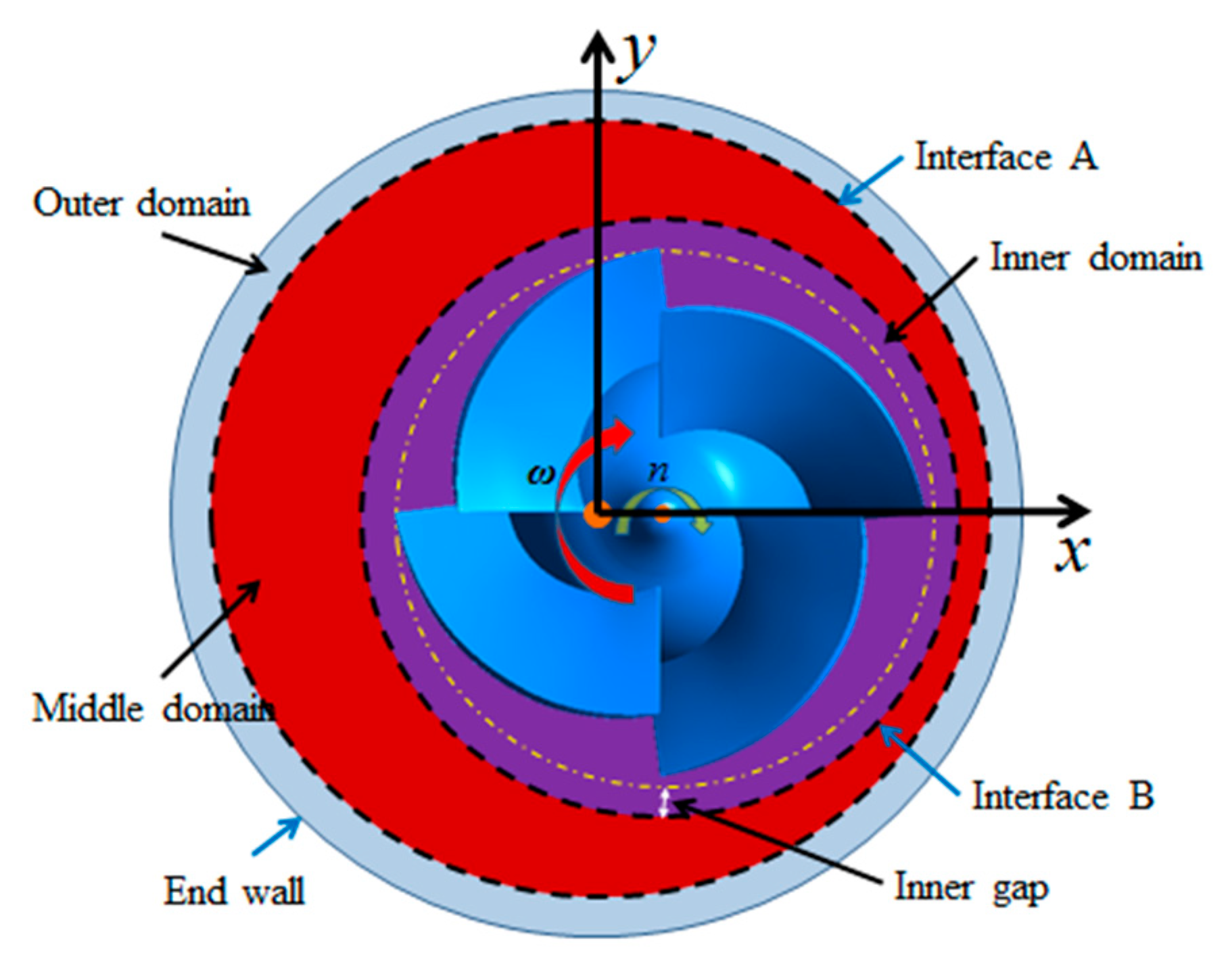
Although the dynamic mesh method can solve the movement of the grid boundary caused by the impeller vortex, the existing dynamic mesh technology requires further improvements. When the mesh reconstruction model in the dynamic mesh model (DM) is used to simulate the clearance flow field of the eccentric impeller, the mesh updating speed cannot keep up with the impeller rotation speed, resulting in mesh distortion and suspension of calculation. Therefore, to load the vortex effect of the eccentric impeller on the eccentric impeller, this paper draws lessons from the “dynamic sliding region (DSR)” proposed by Wang Leqin and Li Zhifeng [36,37] when simulating the transient flow field at the runner start-up. A “dynamic sliding multi-region (DSMR)” method is proposed to simulate the three-dimensional eccentric rotating impeller. The multi-region dynamic sliding method divides the simulation region into three regions, as shown in Figure 3. The water domain of the impeller is the inner domain, the region loaded with the vortex effect is the middle domain, and the boundary layer region is the outer domain; the relative motion reference of the inner region is set as the middle region through the mesh motion mode in ANSYS fluent 15.0. A slip interface connects each region, and the data transmission between non-coincident grid nodes is realized by interface flux interpolation.
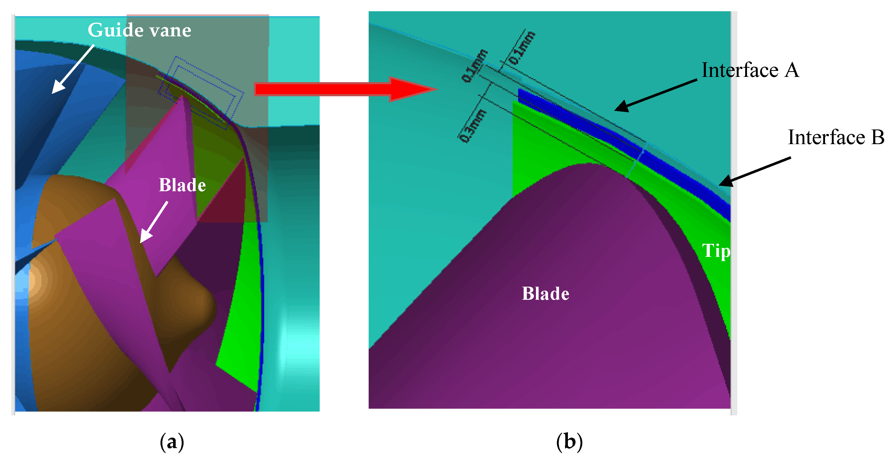
Since the tip clearance of the mixed-flow pump is 0.8 mm, the water area clearance in the inner area under the 0.3 mm eccentricity parameter is set to 0.1 mm. The water area clearance in the inner area under the 0.5 mm eccentricity parameter is set to 0.3 mm. Under the two eccentricity parameters, the minimum gap between the middle and outer areas is set to 0.1 mm, as shown in Figure 4.
3.3. Mesh Generation and Boundary Conditions
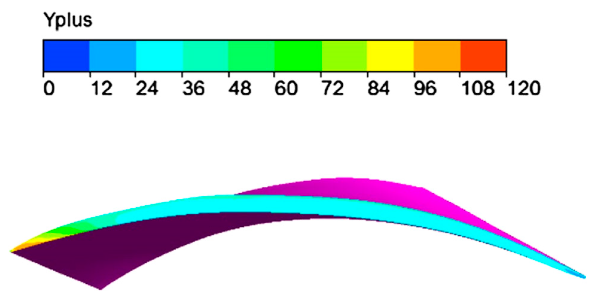
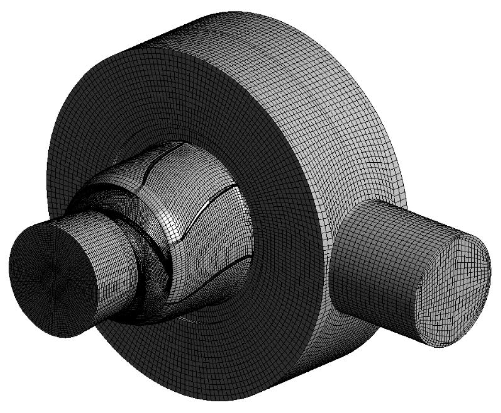
Since the physical model of the mixed-flow pump includes an inlet section, impeller section, guide vane section, annular volute chamber section, and outlet section, therefore, in the meshing, the inlet section, impeller, guide vane, volute chamber, and outlet section of the mixed-flow pump model are discretized, respectively. ICEM software is very convenient for the meshing of complex geometry. It can use J/O and H/O topology for structural meshing, so ICEM software carries the hexahedral structure meshing of different waters. Due to the multi-region dynamic sliding method, the impeller is divided into three water areas for grid division and finally assembled into an integral impeller section grid. In the simulation, it is necessary to consider the influence of the boundary layer mesh on the blade surface, so, we encrypt the grid on the blade surface and adopt J/O topology in the water area in the impeller section to make the grid close to the blade. To ensure enough grids in the blade tip gap, the two boundary layer water areas are densified by controlling the grid nodes in the middle and outer areas. The grid y+ value in the gap area is controlled to change within 100, which meets the requirements of the turbulence model for y+ near the wall; the y+ value of the blade tip is shown in Figure 5 [38]. Similarly, the grid near the guide vane is encrypted. Since the guide vane structure is more straightforward than the blade structure, the guide vane water area adopts H/O topology, and the structured grid of the mixed-flow pump is shown in Figure 6. The inner region of the impeller water region is set as the rotation region, the middle region is set as the revolution region, and the outer region is set as the boundary layer region, which realizes the eccentric vortex rotation of the mixed-flow pump. Set the boundary conditions for numerical calculation, as shown in Table 1.
3.4. Grid Independence Analysis
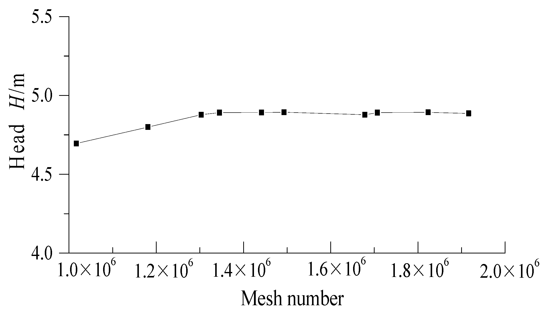
In this paper, the independence of the grid number of the mixed-flow pump under the design condition and steady flow is tested, and the calculated speed is 1450 r/min. Using the same grid topology, the grid quality is consistent by changing the number of grid nodes on the topology line and adjusting the corresponding nodes. Figure 7 shows the head when the eccentricity is 0.3 mm calculated using the same control equation and boundary conditions. It can be seen from the figure that when the number of global calculation grids reaches 1.68 million, the change of calculation head by increasing the number of grids is minimal, and the error is within ±5%, which meets the requirements of the grid independence test.
4. External Characteristic Test Verification
4.1. Test Device and Test Method
To verify the accuracy of the numerical simulation, a test device, as shown in Figure 8, is built to measure the mixed-flow pump’s external characteristics and compare them with the numerical calculation results. The ZJ torque and a speed measuring instrument with an accuracy of 0.2 is used for the torque measurement of the model pump, an LWGY turbine flowmeter with an accuracy of 0.5 is used for the flow measurement, and a WT-1151 pressure transmitter with an accuracy of 0.2 is used for the inlet and outlet pressure measurement. The test bench meets the accuracy requirements of level 1, and the change of working conditions is realized by adjusting the opening of the regulating valve on the outlet pipeline. The energy data collected by the HSJ2010 hydraulic machinery comprehensive tester is transmitted to the computer, and the obtained data are sorted and post-processed.
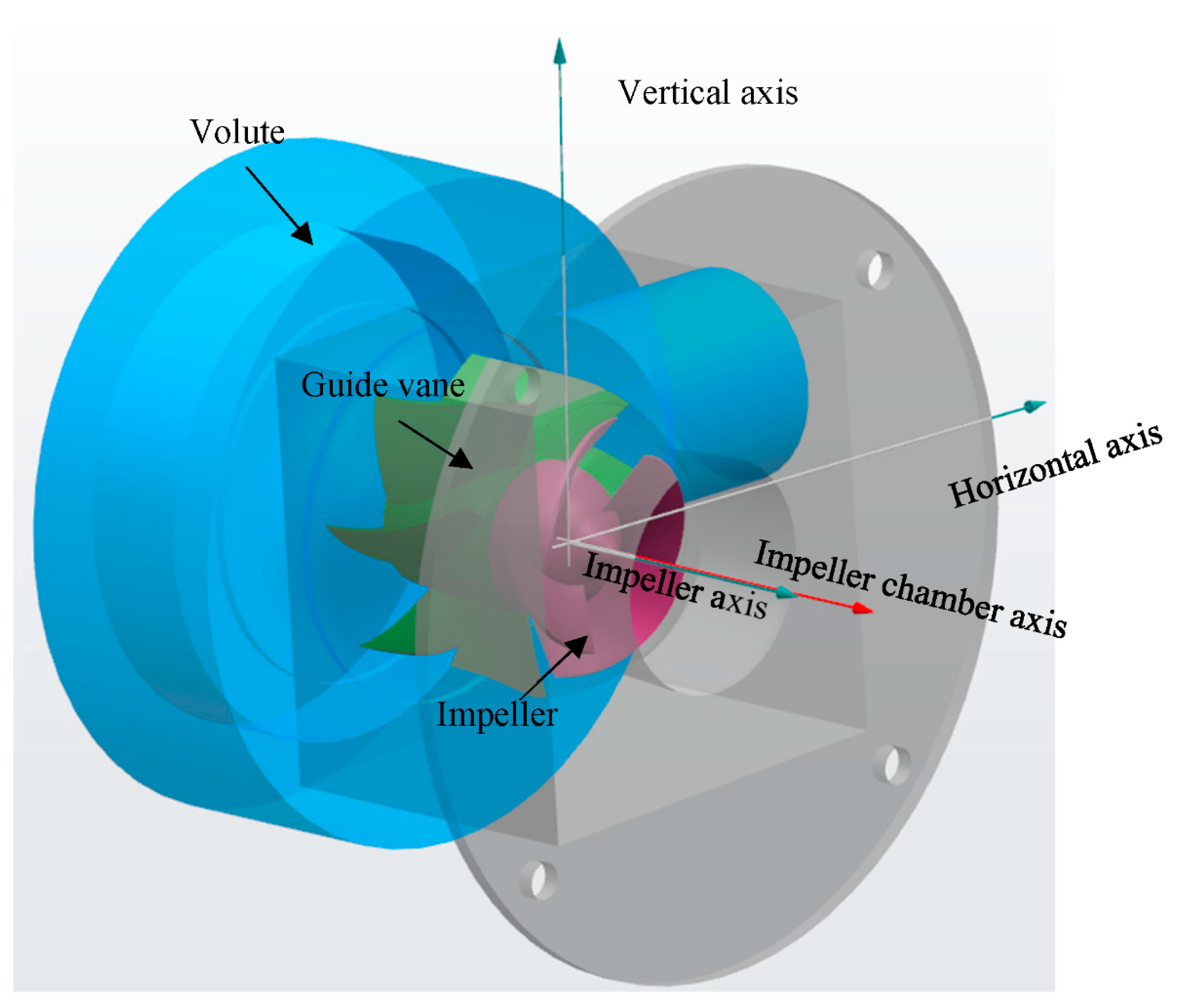
In the test, it is difficult to adjust the eccentricity of the mixed-flow pump rotor directly, and the existence of eccentricity and its rotation will produce significant circumferential unbalanced force during the rotation of the mixed-flow pump. This force is challenging to measure dynamically, which can lead to instability during the operation of the mixed-flow pump, and there are significant potential safety hazards. Therefore, to ensure the test safety and the stability of mixed-flow pump unit operation, the eccentricity can be adjusted by changing the relative position of the impeller and impeller cavity axis. Figure 9 is the installation diagram of the impeller and impeller chamber. For example, when the eccentricity is 0 mm, the axis of the impeller and the impeller chamber coincide. When the eccentricity is 0.3 mm, the axial distance between the impeller and the impeller chamber is adjusted to 0.3 mm. Adjust the installation position of the center of the processed transparent runner chamber to a distance of 0.3 mm in the horizontal direction relative to the axial line of the impeller. At this time, the maximum and minimum dimensions will appear when measuring the tip clearance in the horizontal direction. The tip clearance in the vertical direction should be the same size. In this case, the eccentric adjustment is the most accurate. When the eccentricity is adjusted to 0.5 mm, carry out the same steps.
Before the test, first, adjust the opening of the outlet valve of the test bench to the maximum, start the frequency converter, and adjust the frequency of the frequency converter to stabilize the speed of the mixed-flow pump at 1450 r/min; then, gradually reduce the opening of the outlet valve, and successively record the energy performance parameters of the mixed-flow pump under different flow conditions. When the outlet valve is closed, stop the motor and repeat the above test after the fluid in the pipeline is stabilized. After measuring the inlet and outlet pressure of the pump, the pump head can be calculated by Equation (6). In the test, the pump is installed horizontally, and its inlet and outlet heights are at the same horizontal height, so Z2 = Z1. The diameters of the pump inlet and outlet are known, and the average flow rate v2 and v1 at the pump inlet and outlet can be calculated by the following formula:
where H represents the head, m; p2 and p1 represent the pump outlet and inlet pressure, respectively, Pa; ρ is water density, ρ = 998 kg/m3; g is gravitational acceleration, g = 9.8 m/s2; v2 and v1 are the average flow rate of the pump inlet and outlet, respectively, m; Z2 and Z1 are the installation height of the pump inlet and outlet, respectively, m.
The shaft power P can be calculated from the following formula:
where M is shaft torque, N·m; M0 is no-load torque, N·m; n is rotating speed.
The model pump efficiency η can be calculated from the following formula:
where Q is the flow rate, m3/h; P is the shaft power, kW.
4.2. Comparison of External Characteristics
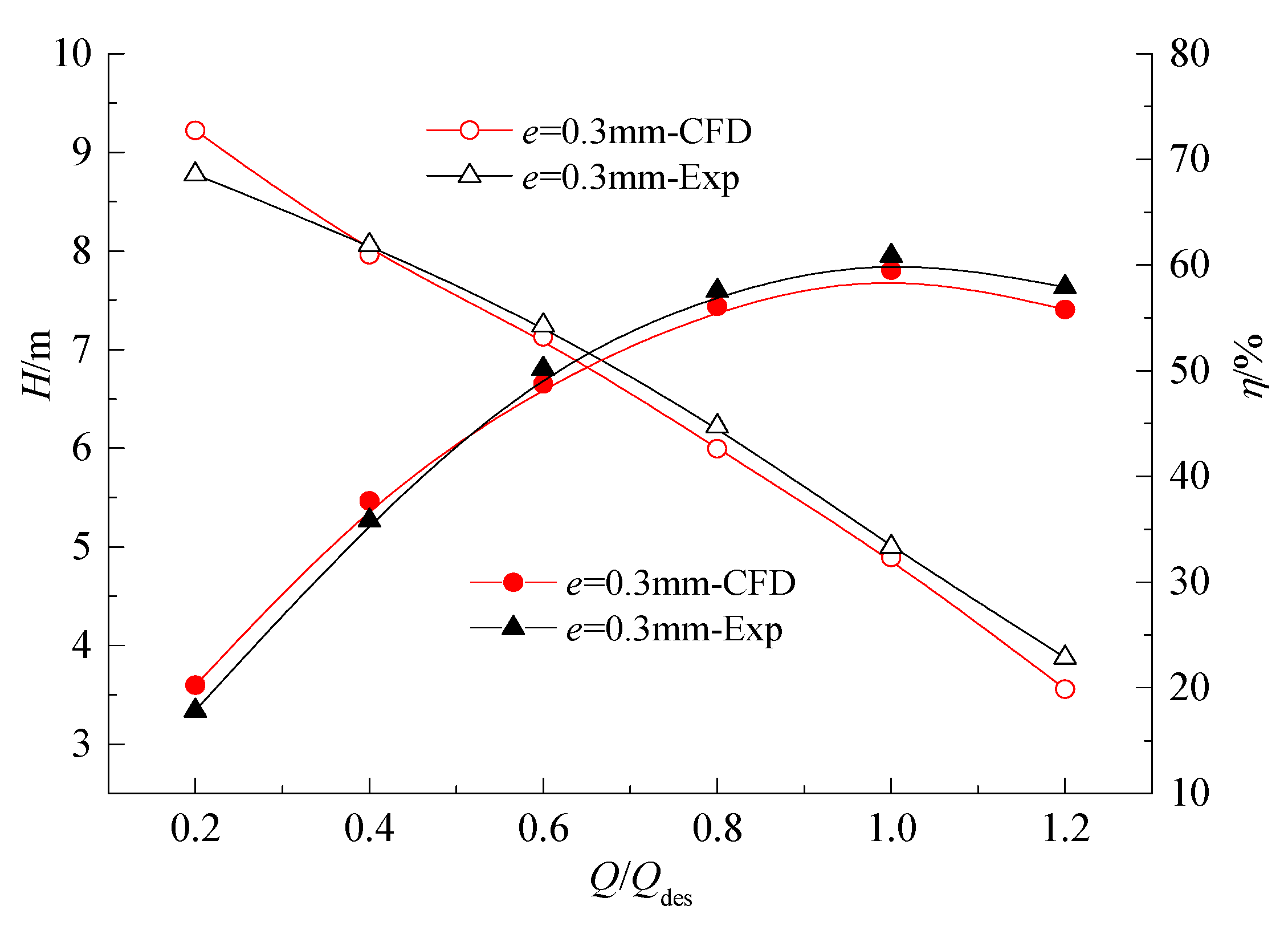
When the eccentricity e = 0.3 mm is obtained, the comparison curve between the predicted external characteristic results of numerical calculation and the test external characteristic results is shown in Figure 10. It can be seen from the figure that the external characteristic results of the numerical calculation are consistent with the trend of test measurement results. Under different flow conditions, the numerical calculation results are in good agreement with the test data. However, because the numerical calculation considers the whirl of the eccentric impeller, and the test only sets the physical eccentricity, the test head is greater than the calculated head. However, under the condition of low flow, the calculated head is slightly higher than the test head, the head error at the design flow condition point is about 5%, and the efficiency error is no more than 3%.
5. Vortex Dynamics Analysis of Flow Field under Alford Effect
5.1. Streamline of Tip Region with Different Eccentricities
Figure 11 shows the three-dimensional streamline at the tip clearance under different eccentricities. The tip leakage flow is almost the same at the tip clearance of each blade. In the part near the tip suction surface, the initial leakage flow intensity is high, andthe speed is significant. Then, the intensity gradually weakens, the speed decreases, and a low-speed zone appears near the tip pressure surface of the next blade. When the impeller is eccentric, the leakage flow characteristics of each blade tip are quite different. In the eccentric state, the low-speed region formed by tip leakage flow at blade A and blade B at the maximum clearance is the largest. The low-speed region at the maximum clearance becomes more significant with the increase of eccentricity. At the minimum clearance, the tip leakage flow at blade C and blade D is the smallest, and the low-speed zone at the minimum clearance decreases with the increase of eccentricity. In general, the eccentricity will have a significant impact on the leakage flow in the impeller clearance. The greater the eccentricity, the more pronounced the non-uniformity of the leakage flow in the impeller clearance.
5.2. Vortex Core Extraction in Eddy Flow Field
The vortex structure in the flow field determines many properties of the flow field and plays an essential role in hydrodynamics. It is vital to judge the vortex structure from such complex data. In this paper, the Q-criterion method is used to identify the vortex structure of the flow field under the Alford effect.
The Q criterion defines the second matrix invariant Q of velocity gradient tensor ∇V in the flow field. The region with a positive value is the vortex, and the pressure in the vortex region is lower than the surrounding pressure.
For incompressible flow, ∇·V = 0, the above formula can be rewritten as
where Ω and S are the antisymmetric and symmetric parts of the velocity gradient tensor matrix, representing the deformation and rotation of a point in the flow field, respectively, S is the strain rate tensor, and Ω is the rotation tensor. It can be seen from the above formula that the Q criterion reflects a balance between the rotation and deformation of a fluid micro cluster in the flow field. Q > 0 reflects the dominance of rotation inflow. In addition, the Q criterion requires an additional condition that the pressure at this point is the minimum value of the nearby region. According to the N-S equation, the Poisson equation of pressure can be written as follows
According to the extreme value theorem, Q > 0 makes the maximum pressure only on the boundary, but it cannot guarantee that the minimum pressure is in the region.
5.2.1. Vortex Identification in Impeller
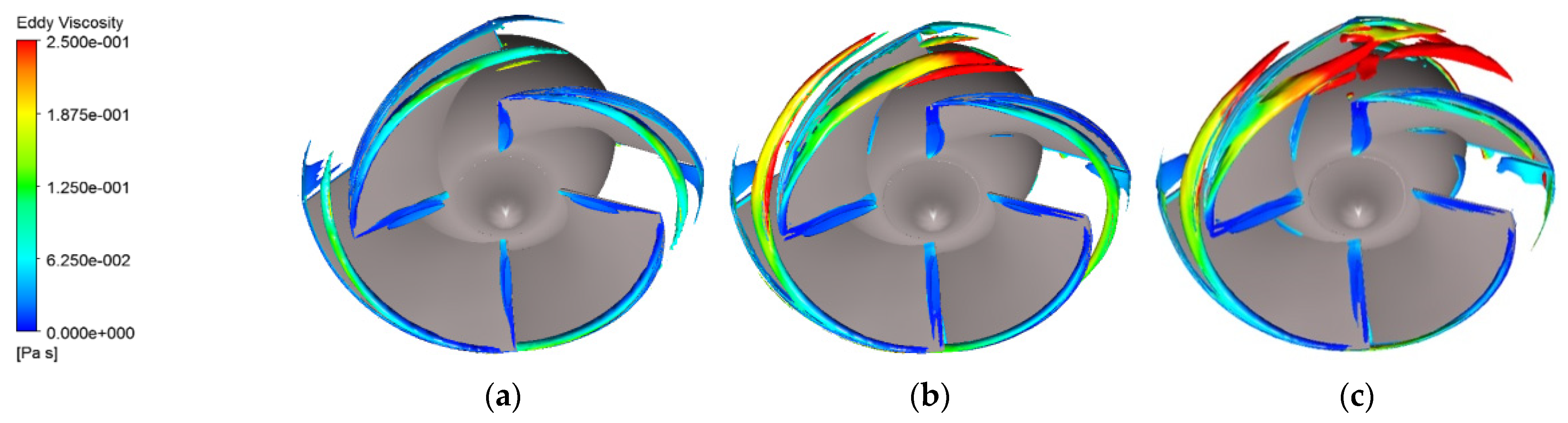
Figure 12 shows the distribution of vortex cores in the impeller under three eccentricity parameters under design conditions, and the lower side of the impeller is the side of the impeller. It can be seen from the figure that the vortex core distribution in the internal flow field of the non-eccentric impeller is stable, the vortex core is attached to the tip of each blade, and the leakage vortex formed by the leakage flow is symmetrically distributed in the impeller channel. At the same time, at the leading edge of the blade suction surface, a specific region of separation vortex is generated due to flow separation. Under the eccentricity of 0.3 mm and 0.5 mm, the distribution of the vortex core in the impeller is asymmetric. Under the small tip gap, the strength and distribution area of the vortex core increase significantly, and the flow field in the impeller channel becomes more unstable. In addition to the vortex generated by leakage flow and flow separation, there is also a vortex structure formed by secondary flow in the channel. Under the large tip gap, the strength and influence region of the vortex core is reduced. Compared with the small eccentricity parameter, under the significant eccentricity parameter, the vortex structure in the impeller channel and at the blade outlet increases significantly, indicating that the increase of eccentricity makes the flow in the impeller flow field more unstable, and the fluid energy loss increases, so the lift and efficiency corresponding to the external characteristic curve decrease.
5.2.2. Vortex Identification in Guide Vane
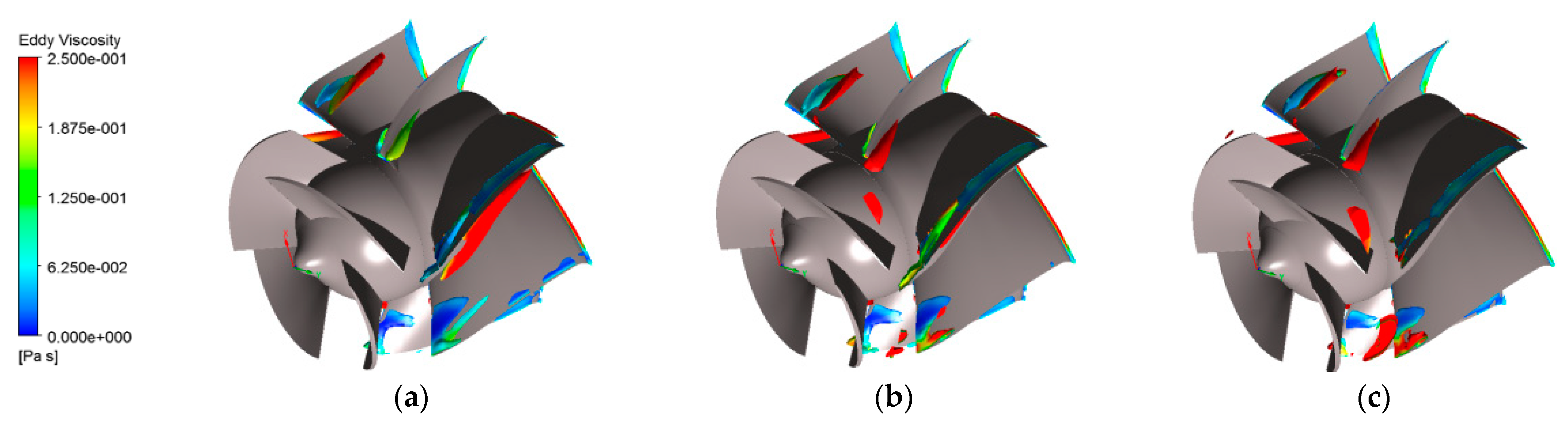
Figure 13 shows the vortex core distribution in the guide vane under three eccentricity parameters under design conditions. It can be seen from the figure that there is little difference in the distribution of vortex cores in the guide vane under the three eccentricities. Still, the vortex strength in the guide vane is small without eccentricity parameters. There are some scattered vortex structures at the guide vane inlet under eccentricity, which is different from the impeller flow field under non-eccentricity. At the same time, with the increase of eccentricity parameters, the strength of the vortex core structure gradually increases, and the number also increases obviously. Obvious flow separation occurs near the inlet of the guide vane suction surface on the eccentric side of the impeller, and the vortex structure is attached to the guide vane tip. At the same time, the vortex structure scattered from the impeller outlet appears in the channel at the guide vane inlet, which blocks the guide vane channel. However, due to the rectification effect of the guide vane, there are few vortex structures at the guide vane outlet. In general, under the three eccentricity parameters, the distribution of vortex cores in the guide vane increases with eccentricity. Still, due to the geometric structure and action of the guide vane, the vortex structure at the outlet of the guide vane decreases obviously in each state.
5.3. Stress Analysis of Vortex Flow Field
Based on the vorticity moment theory and the finite domain theory reflecting the local hydrodynamic characteristics of the near-field fluid, the stress of blade under non-uniform blade tip clearance is analyzed, and the key parameters affecting blade thrust and hydraulic efficiency are studied. The internal of the mixed-flow pump is complex turbulent flow. According to the idea of eddy viscosity model in turbulence model theory, the influence of turbulent Reynolds stress is expressed by turbulent viscosity coefficient, and considering the absence of acceleration motion of a solid wall, the simplified formula of the dynamic vorticity moment is:
The hydrodynamic moment is mainly composed of two parts, the first-order moment of tangential vorticity and the second-order moment of tangential vorticity flow, which respectively reflect the effect of surface shear stress and pressure, which are called L1 and L2, respectively.
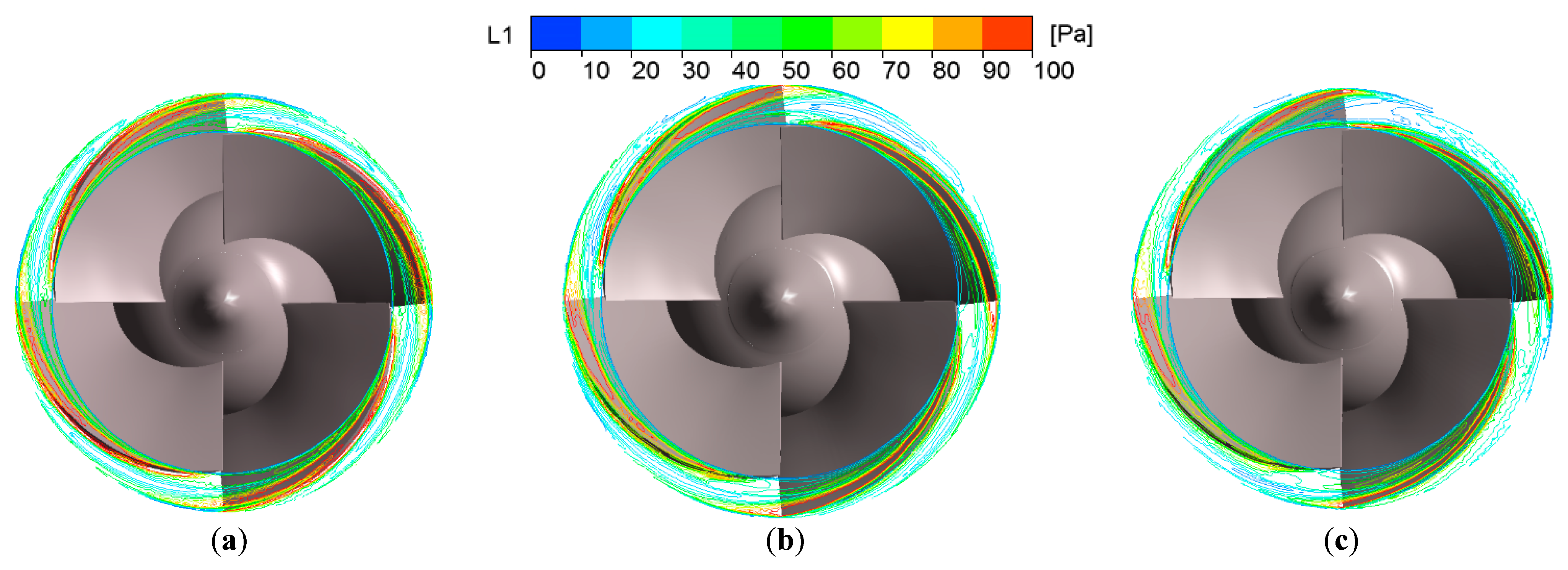
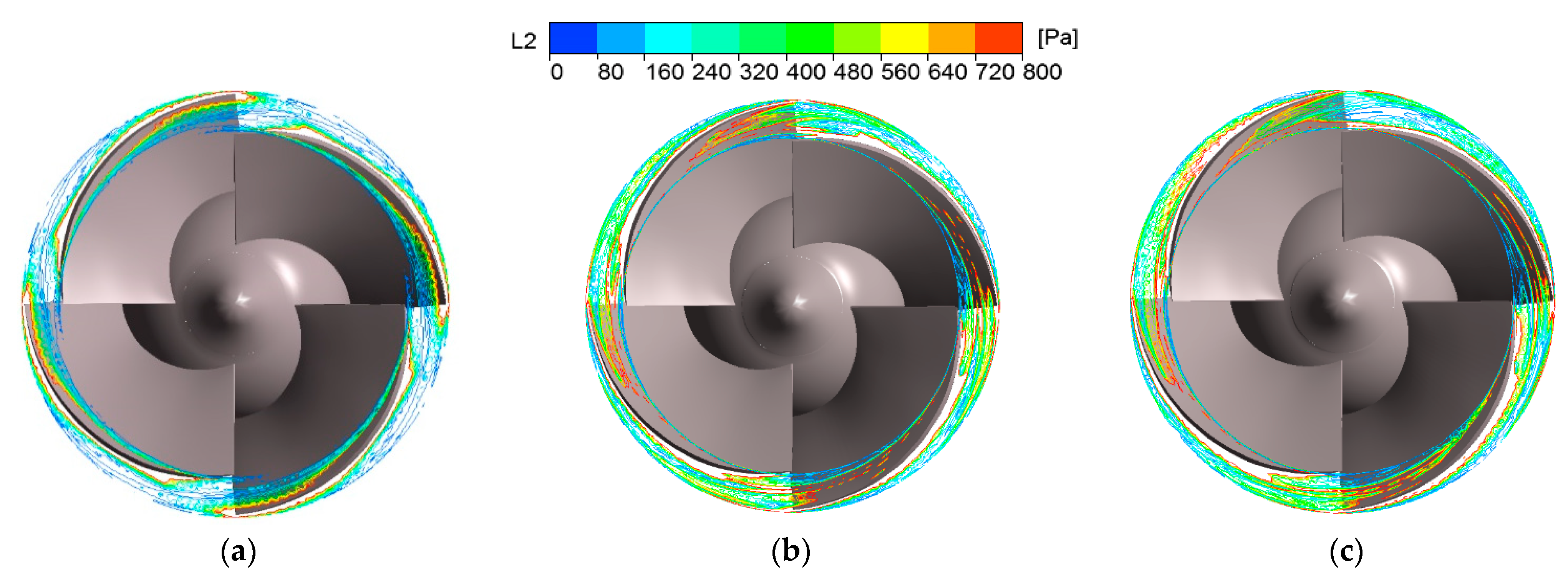
Figure 14 shows the contour map of the distribution of friction L1 in the end wall area of the impeller blade under three eccentricity parameters under design conditions (the left side is the eccentric impeller biased to one side). It can be seen from the figure that under different eccentricity parameters, there is a high L1 value at the rim of the impeller blade, indicating that the shear force in this area is apparent. The area with a high L1 value distribution of rim clearance of the non-eccentric impeller is distributed in a thin strip shape, with a long circumferential size and symmetrical circumferential direction, covering almost the whole blade rim. However, under the eccentricity of 0.3 mm and 0.5 mm, the area with high L1 value distribution is significantly reduced; it is basically located in the middle and rear of the blade, and the distribution width increases slightly, the whole is an elliptic ring with a long axis. At the same time, in the eccentric state, the value of L1 at the small gap is significantly higher than that at the large gap, and the area of high L1 distribution at the small gap is wide, but the length is reduced. It can be seen that under the eccentric state, the impeller tip is the area where the fluid high shear stress is concentrated. At the same time, at different gaps, the distribution difference of the L1 value representing friction is significant, and the impeller is affected at small gaps.
Figure 15 shows the distribution contour map of pressure L2 in the end wall area of the impeller blade under three eccentricity parameters under design conditions (the left side is the eccentric impeller biased to one side). It can be seen from the figure that compared with the distribution of L1 in the end wall area, the difference of the L2 distribution contour map is more apparent, and the value distribution range of L2 in the end wall area is also increased. However, similar to L1 distribution, the value distribution of blade tip clearance L2 of the non-eccentric impeller is circumferential symmetrical. In contrast, under the eccentricity of 0.3 mm and 0.5 mm, the value of L2 varies significantly at the blade tip of left and right impellers. Under the two eccentric states, the L2 value distribution in the end wall area is similar, but the high L2 value area at the small gap is more significant than that at the large gap. At the same time, the range of this area also increases slightly under the significant eccentricity parameter. It can be seen that eccentricity increases the fluid pressure in the impeller, in which the fluid in the clearance area is greatly affected. In contrast, the increase of eccentricity significantly increases the pressure effect of unsteady fluid in the end wall area of the impeller, and the Alford force in the tip clearance increases.
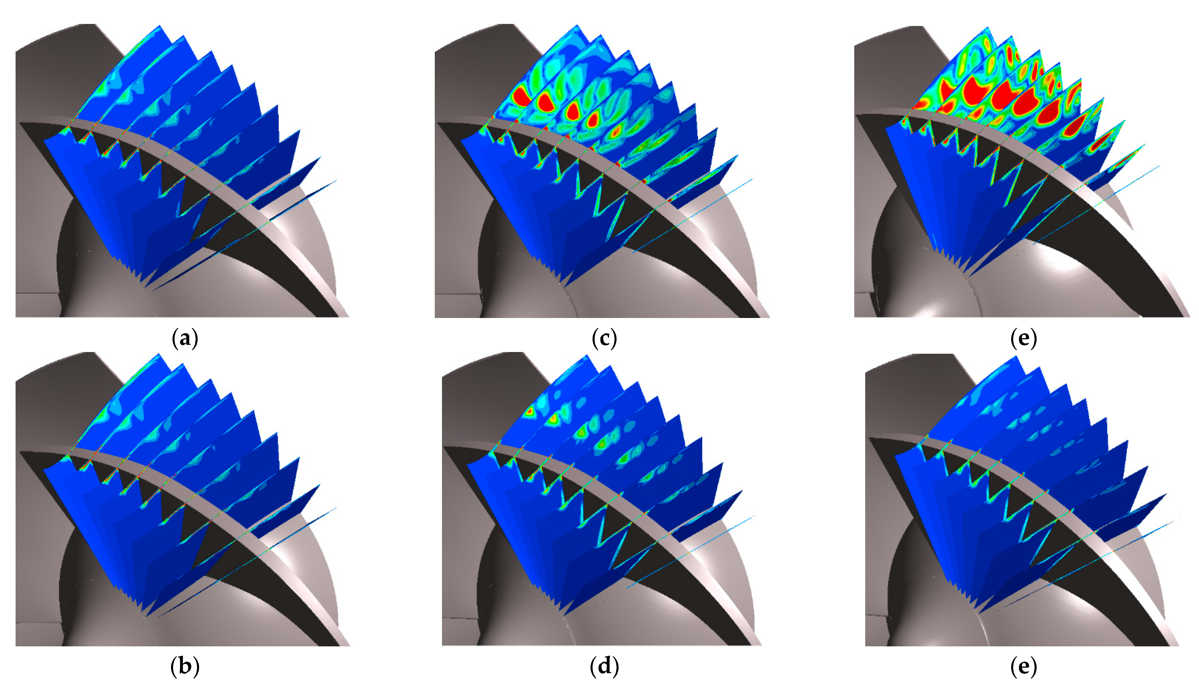
To compare the distribution of L1 and L2 in the impeller passage along the span direction of the blade, the cloud diagram distribution of the blade along the span direction on the eccentric side and non-eccentric side of the impeller under different eccentricity parameters under the design condition is intercepted, as shown in Figure 16 and Figure 17. It can be seen from the figure that under the design flow condition, the distribution of L1 and L2 at different gaps in the eccentric impeller is different, while the flow field of the non-eccentric impeller is also symmetrically distributed due to the circumferential symmetry of the impeller blade tip gap. The values of L1 and L2 at the small blade tip clearance are significantly higher than those at the ample clearance, indicating that the large torque caused by the flow field is the root cause of abnormal vibration of the impeller at the small clearance. At the ample clearance, the values of L1 and L2 are low, and the extreme value is far away from the blade pressure surface, which has little impact on the blade. At the small blade tip clearance, L1 and L2 values increase significantly with the increase of eccentricity. Along the blade span direction, the values of L1 and L2 under different eccentricity parameters decrease. At the small blade tip clearance, the areas with the high-value distribution of L1 and L2 deviate from the blade pressure surface. The areas along with the span direction decrease, indicating that the areas before the blade inlet and the middle of the blade are greatly affected by the eccentricity parameters.
In contrast, the flow field at the blade outlet is less affected by the eccentricity. The leading edge region of the blade is the central part affected by the unstable torque of the flow field. In summary, the flow field in the impeller is stable without eccentricity, and the values of the components L1 and L2 of the vorticity moment are small. However, in the eccentric state, the values of L1 and L2 at the slight gap increase with eccentricity. The Alford moment on the impeller increases; the values of L1 and L2 gradually decrease along the blade span. The blade’s leading edge is the main force part, and the torque of the eccentric flow field has little effect on the blade outlet.
5.4. Impacting Depth of TLF with Different Eccentricities
The impact depth of tip leakage flow under different eccentricities is compared and analyzed by monitoring the pressure values of different span curves. To eliminate the influence of location factors on the value, the pressure coefficient Cp is used to process the pressure data dimensionless, which is shown as Equation (15),
where p is the static pressure at the point of the calculated pressure coefficient; p∞ is the independent static pressure away from any disturbance; p0 is the independent stagnation pressure away from any disturbance.
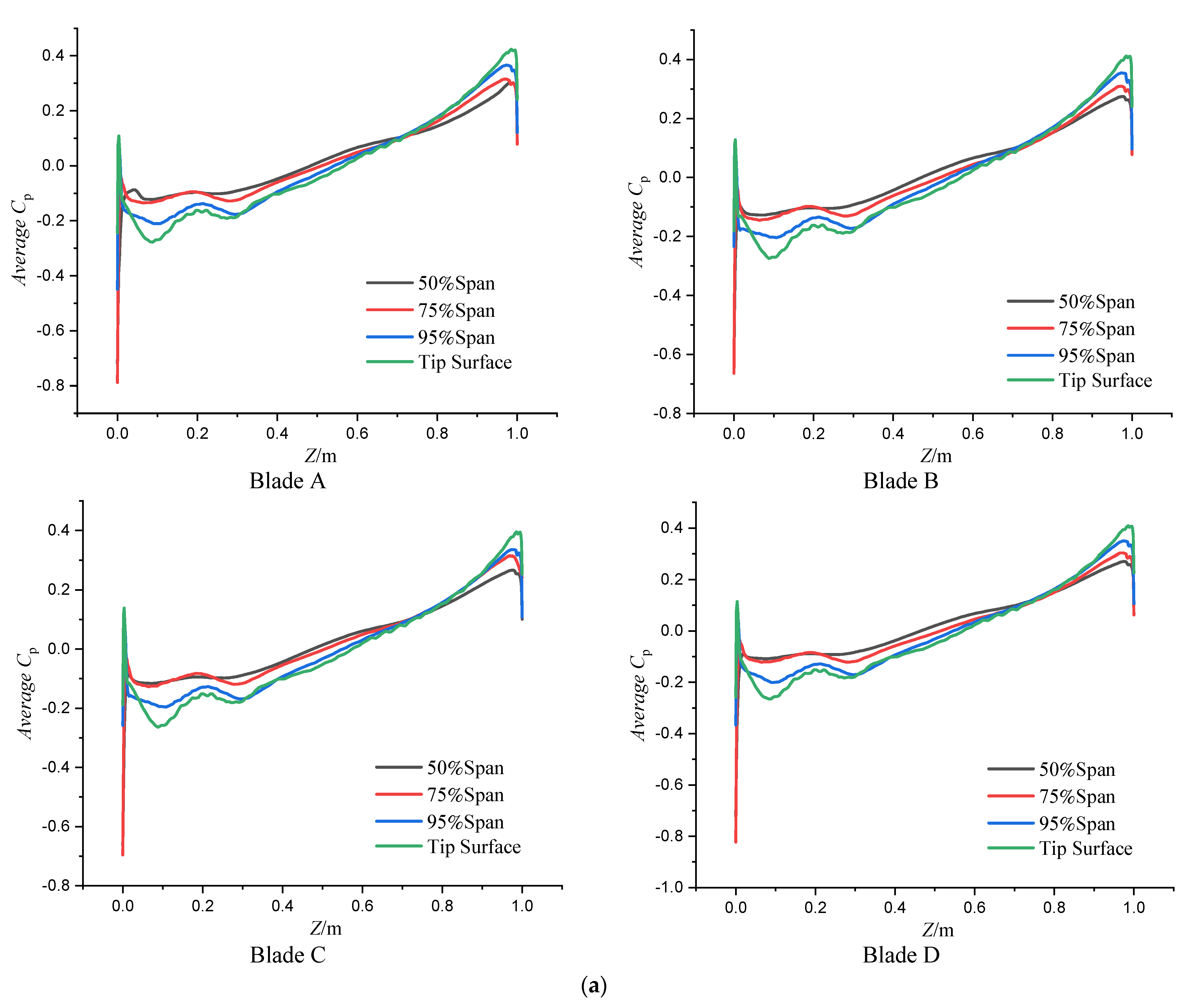
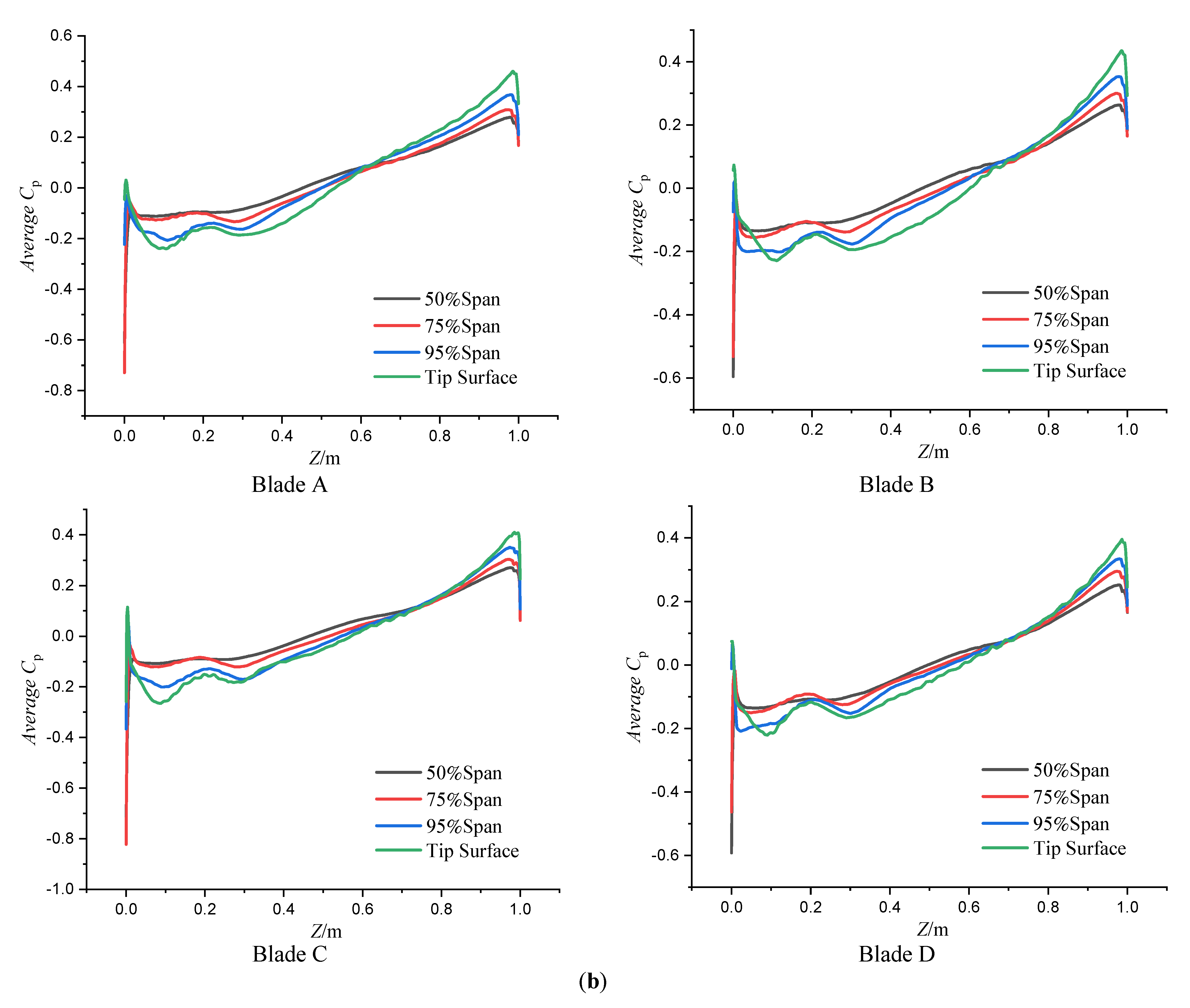
To more intuitively show the change of pressure data, the pressure coefficient Cp is numerically averaged. Figure 18 shows the mean pressure coefficient curves of 50% span, 75% span, 95% span, and the blade tip surface under different eccentricities, and Z in the figure represents the distance along the axis. When the eccentricity e = 0 mm, the pressure coefficients on the four blades are the same. The mean pressure coefficient curve changes significantly when eccentricity occurs, especially in the mean pressure coefficient curve on the blade tip surface. When the eccentricity e = 0.3 mm, the pressure coefficient of the blade B tip surface decreases significantly, but the pressure coefficient of 50% span, 75% span and 95% span surface changes little, which indicates that the impact depth of the tip leakage flow is shallow and only has a significant impact on the tip surface area. However, when the eccentricity reaches e = 0.5 mm, the pressure coefficient curves of blade D at 75% span, 95% span surface, and tip surface change, indicating that the impact depth of tip leakage flow is deepened, which has a particular impact on the blade inlet flow field, the 50% span surface pressure coefficient has little change, indicating that the impact area of clearance leakage flow is mainly concentrated in the first half of the impeller channel, which has little impact on the blade outlet flow field, which is the same as that shown in Figure 16 and Figure 17.
6. Conclusions
- (1)
- A multi-region dynamic sliding method is established, and the numerical simulation of the three-dimensional eccentric rotating impeller of the mixed-flow pump is carried out. They were comparing the results of numerical simulation and external characteristics of the test, when the eccentricity e = 0.3 mm, the numerical calculation results are in good agreement with the test data. The head error of the design flow operating point is about 5%, the efficiency error is no more than 3%, and the accuracy of numerical calculation is high.
- (2)
- With the increase of eccentricity, the vortex structure in the impeller channel and at the blade outlet increases significantly, and the strength and number of vortex core structures in the guide vane also increase significantly, the increase of eccentricity makes the flow in the impeller flow field more unstable, and the energy loss of fluid increases. Apparent flow separation occurs near the inlet of the guide vane suction surface on the eccentric side of the impeller, and the vortex structure is attached to the guide vane tip.
- (3)
- The values of vorticity moment components L1 and L2 increase with the increase of eccentricity, and the Alford moment on the impeller increases. Along the blade span direction, the values of L1 and L2 gradually decrease. The leading edge of the blade is the main force part, and the Alford effect is significant, while the torque of the eccentric flow field has little effect on the blade outlet.
- (4)
- With the increase of eccentricity, the impact degree of tip leakage flow deepens, the surface pressure of each span changes in varying degrees, and the change of tip surface pressure is the most obvious. At large eccentricity, the impact area of tip leakage flow is mainly concentrated in the first half of the impeller channel, which will impact the blade inlet flow field and have less impact on the blade outlet flow field.
Author Contributions
Conceptualization, W.L.; data curation, L.J.; writing—original draft preparation, S.L.; writing—review and editing, S.L., W.L., W.S. and R.K.A. All authors have read and agreed to the published version of the manuscript.
Funding
This research was funded by the Key International Cooperative research of National Natural Science Foundation of China (No. 52120105010), National Natural Science Foundation of China (No. 52179085), the National Key R&D Program Project (No. 2020YFC1512405), the Fifth “333 High-Level Talented Person Cultivating Project” of Jiangsu Province, Funded projects of “Blue Project” in Jiangsu Colleges and Universities.
Institutional Review Board Statement
Not applicable.
Informed Consent Statement
Not applicable.
Data Availability Statement
The data used to support the findings of this study are included within the article.
Conflicts of Interest
The authors declare no conflict of interest.
References
- Alford, J.S. Protecting Turbomachinery from Self-excited Rotor Whirl. J. Eng. Power 1965, 87, 333–343. [Google Scholar] [CrossRef]
- Thomas, H.J. Unstable Natural Vibration of Turbine Rotors Induced by the Clearance Flow in Glands and Blading. Bull. L’AIM 1958, 71, 1039–1063. [Google Scholar]
- Kim, H.S.; Cho, M.H.; Song, S.J. Stability Analysis of a Turbine Rotor System with Alford Forces. J. Sound Vib. 2003, 260, 167–182. [Google Scholar] [CrossRef]
- Kang, Y.-S.; Kang, S.-H. Prediction of the Nonuniform Tip Clearance Effect on the Axial Compressor Flow Field. ASME J. Fluids Eng. 2010, 132, 051110. [Google Scholar] [CrossRef]
- Nandi, S.; Ahmed, S.; Toliyat, H. Detection of rotor slot and other eccentricity related harmonics in a three phase induction motor with different rotor cages. Energy Convers. IEEE Trans. 2001, 16, 253–260. [Google Scholar] [CrossRef]
- Brennen, C.E. Hydrodynamics of Pumps; Concepts NREC: White River Junction, VT, USA; Oxford University Press: London, UK, 2011; pp. 203–205. [Google Scholar]
- Moore, J.; Palazzolo, A. Rotordynamic Force Prediction of Whirling Centrifugal Impeller Shroud Passages using Computational Fluid Dynamic Techniques. ASME J. Eng. Gas Turbines Power 2001, 123, 910–917. [Google Scholar] [CrossRef] [Green Version]
- Shinichiro Hata, J.R. The Effects of Casing Geometry and Flow Instability on Rotordynamic Fluid Forces on a Closed Type Centrifugal Impeller in Whirling Motion. In Proceedings of the ASME-JSME-KSME 2011 Joint Fluids Engineering Conference: AJK2011-06022, Hamamatsu, Japan, 24–29 July 2011; Volume 1, pp. 113–119. [Google Scholar]
- Li, W.; Ji, L.; Shi, W.; Zhang, Y. Numerical calculation of non-uniform rim clearance flow field in mixed flow pump. Trans. Chin. Soc. Agric. Mach. 2016, 47, 66–72. [Google Scholar]
- Shoji, H.; Ohashi, H. Lateral Fluid Forces on Whirling Centrifugal Impeller (1st Report:Theory). ASME J. Fluid Eng. 1987, 109, 94–99. [Google Scholar] [CrossRef]
- Adkins, D.R.; Brennen, C.E. Analyses of Hydrodynamic Radial Force on Centrifugal Pump Impellers. ASME J. Fluid Eng. 1988, 110, 20–28. [Google Scholar] [CrossRef]
- Ji, L.; Li, W.; Shi, W.; Tian, F.; Agarwal, R. Diagnosis of internal energy characteristics of mixed-flow pump within stall region based on entropy production analysis model. Int. Commun. Heat Mass Transf. 2020, 117, 104784. [Google Scholar] [CrossRef]
- Zhou, L.; Shi, W.; Cao, W.; Yang, H. CFD investigation and PIV validation of flow field in a compact return diffuser under strong part-load conditions. Sci. China Technol. Sci. 2015, 58, 405–414. [Google Scholar] [CrossRef]
- Li, W.; Jiang, X.; Pang, Q.; Zhou, L.; Wang, W. Numerical simulation and performance analysis of a four-stage centrifugal pump. Adv. Mech. Eng. 2016, 8, 1–8. [Google Scholar] [CrossRef] [Green Version]
- Lei, T.; Zhiyi, Y.; Yun, X.; Yabin, L.; Shuliang, C. Role of blade rotational angle on energy performance and pressure fluctuation of a mixed-flow pump. Proceedings of the Institution of Mechanical Engineers. Part A J. Power Energy 2017, 231, 227–238. [Google Scholar] [CrossRef]
- Chochua, G.; Soulas, T.A. Numerical Modeling of Rotordynamic Coefficients for Deliberately Roughened Stator Gas Annular Seals. ASME J. Tribol. 2007, 129, 424–429. [Google Scholar] [CrossRef]
- Zhang, L.; Liu, S.; Wu, Y. Vorticity dynamics analysis of flow field in Francis runner. J. Hydroelectr. Eng. 2007, 26, 106–110. [Google Scholar]
- Li, F.; Fan, H.; Wang, Z.; Chen, N. Optimum design of runner blades of a tubular turbine based on vorticity dynamics. J. Tsinghua Univ. 2011, 51, 836–839. [Google Scholar]
- Zhaohui, X. The Analysis of Three-Dimensional Flow in High-Speed Pump and Research of Its Fluid-Induced Pressure Fluctuation; Tsinghua University: Beijing, China, 2004. [Google Scholar]
- Yang, L.; Fan, H.; Chen, N. Bidirectional flow diagnosis to optimize the design of a pump-turbine runner using vorticity dynamics theory. J. Tsinghua Univ. 2007, 47, 686–690. [Google Scholar]
- Fan, H.; Chen, N.; Yang, L. Three dimensional flow diagnosis of the pump turbine runner based on the dynamic vorticit. J. Hydroelectr. Eng. 2007, 26, 124–128. [Google Scholar]
- Pan, Z.; Chen, S.; Wu, Y.; Zhang, D.; Li, Y. Study on internal fluid force of centrifugal pump with given rotor dynamics parameters. Trans. Chin. Soc. Agric. Mach. 2013, 44, 55–60. [Google Scholar]
- Huang, S.; Yang, F.; Guo, J.; Qv, G. The unsteady flow of centrifugal pump is simulated by three-dimensional dynamic grid technology. Sci. Technol. Rev. 2013, 31, 33–36. [Google Scholar]
- Jiang, F.; Chen, W.; Wang, Y.; Qv, J. Numerical simulation of internal flow field of centrifugal pump based on moving grid. Fluid Mach. 2007, 35, 20–24. [Google Scholar]
- Liu, H.; Chen, F.; Ma, B. Numerical simulation of valve flow field based on moving grid and UDF Technology. Turbine Technol. 2008, 50, 106–108. [Google Scholar]
- Ji, L.; Li, W.; Shi, W.; Chang, H.; Yang, Z. Energy Characteristics of Mixed-Flow Pump under Different Tip Clearances Based on Entropy Production Analysis. Energy 2020, 199, 1–15. [Google Scholar] [CrossRef]
- Li, W.; Ji, L.; Li, E.; Shi, W.; Agarwal, R.; Zhou, L. Numerical investigation of energy loss mechanism of mixed-flow pump under stall condition. Renew. Energy 2020, 2021, 740–760. [Google Scholar] [CrossRef]
- Li, W.; Li, E.; Ji, L.; Zhou, L.; Shi, W.; Zhu, Y. Mechanism and propagation characteristics of rotating stall in a mixed-flow pump. Renew. Energy 2020, 153, 74–92. [Google Scholar] [CrossRef]
- Ji, L.; Li, W.; Shi, W.; Tian, F. Ramesh Agarwal. Effect of Blade Thickness on Rotating Stall of Mixed-Flow Pump Using Entropy Generation Analysis. Energy 2021, 236, 121381. [Google Scholar] [CrossRef]
- Shixing, C. Study on Internal Fluid Force of Centrifugal Pump with Given Rotor Dynamics Parameters; Jiangsu University: Zhenjiang, China, 2013. [Google Scholar]
- Brennen, C.E.; Acosta, A.J. Fluid-induced rotor dynamic forces and instabilities. Struct. Control Health Monit. 2006, 13, 10–26. [Google Scholar] [CrossRef] [Green Version]
- Zhong, Y.; He, Y.; Wang, Z.; Li, F. Rotor Dynamics; Tsinghua University Press: Beijing, China, 1987. [Google Scholar]
- Li, X.; Liu, C.; Wu, B.; Lv, Y. Numerical simulation of oblique flow pump with single arc space vane based on CFX. Water Resour. Power 2014, 4, 175–179. [Google Scholar]
- Yang, C.; Gao, Q.; Li, Y.; Shen, L. Application of different turbulence models in numerical simulation of mixed-flow pump and its evaluation. J. Lanzhou Univ. Technol. 2014, 40, 51–55. [Google Scholar]
- Siddique, W.; El-Gabry, L.; Shevchuk, I.V.; Fransson, T.H. Validation and Analysis of Numerical Results for a Two-Pass Trapezoidal Channel With Different Cooling Configurations of Trailing Edge. ASME J. Turbomach. 2013, 135, 011027. [Google Scholar] [CrossRef] [PubMed] [Green Version]
- Zhifeng, L. Numerical Simulation and Experimental Study on Transient Flow during Start-Up of Centrifugal Pump; Zhejiang University: Hangzhou, China, 2009. [Google Scholar]
- Wang, L.; Li, Z.; Dai, W.; Wu, D. Two-dimensional numerical simulation of transient flow in centrifugal pump during start-up. J. Eng. Thermophys. 2008, 29, 1319–1322. [Google Scholar]
- Fasquelle, A.; Pellé, J.; Harmand, S.; Shevchuk, I.V. Numerical Study of Convective Heat Transfer Enhancement in a Pipe Rotating Around a Parallel Axis. ASME J. Heat Transfer. 2014, 136, 051901. [Google Scholar] [CrossRef]
Figure 1.
Mixed-flow pump model. (a) Inlet Section; (b) Impeller Section; (c) Guide vane Section; (d) Annular cochlear chamber; (e) Outlet section.
Figure 1.
Mixed-flow pump model. (a) Inlet Section; (b) Impeller Section; (c) Guide vane Section; (d) Annular cochlear chamber; (e) Outlet section.

Figure 2.
Schematic diagram vortex model.

Figure 3.
Schematic diagram of dynamic sliding multi-region method.

Figure 4.
The position of the interface when eccentricity e is 0.3 mm. (a) The position of the domain and interface; (b) The detail of blade tip.
Figure 4.
The position of the interface when eccentricity e is 0.3 mm. (a) The position of the domain and interface; (b) The detail of blade tip.

Figure 5.
y+ of the blade tip region.

Figure 6.
Mesh of the computational area.

Figure 7.
Comparison of the head under different mesh counts.

Figure 8.
Experimental device (a) Motor; (b) Torque meter; (c) Mixed-flow pump; (d) Pressure transmitter; (e) HSJ2010 hydraulic machinery comprehensive data acquisition instrument; (f) Inlet valve; (g) Turbine flow meter; (h) Water tank.
Figure 8.
Experimental device (a) Motor; (b) Torque meter; (c) Mixed-flow pump; (d) Pressure transmitter; (e) HSJ2010 hydraulic machinery comprehensive data acquisition instrument; (f) Inlet valve; (g) Turbine flow meter; (h) Water tank.

Figure 9.
The installation of the impeller chamber and the schematic diagram of the chamber position.
Figure 9.
The installation of the impeller chamber and the schematic diagram of the chamber position.

Figure 10.
The comparison of external characteristics.

Figure 11.
Three−dimensional streamline of tip region under different eccentricities. (a) e = 0 mm; (b) e = 0.3 mm; (c) e = 0.5 mm.
Figure 11.
Three−dimensional streamline of tip region under different eccentricities. (a) e = 0 mm; (b) e = 0.3 mm; (c) e = 0.5 mm.

Figure 12.
Distribution of vortex core in the flow field of tip clearance, (a) e = 0 mm, (b) e = 3 × 10⁻¹ mm, (c) e = 5 × 10⁻¹ mm.
Figure 12.
Distribution of vortex core in the flow field of tip clearance, (a) e = 0 mm, (b) e = 3 × 10⁻¹ mm, (c) e = 5 × 10⁻¹ mm.

Figure 13.
Vortex core distribution in guide vane, (a) e = 0 mm, (b) e = 3 × 10⁻¹ mm, (c) e = 5 × 10⁻¹ mm.
Figure 13.
Vortex core distribution in guide vane, (a) e = 0 mm, (b) e = 3 × 10⁻¹ mm, (c) e = 5 × 10⁻¹ mm.

Figure 14.
Distribution of L1 in runner end wall area with non-uniform tip clearance (span = 0.99). (a) e = 0 mm, (b) e = 3 × 10⁻¹ mm, (c) e = 5 × 10⁻¹ mm.
Figure 14.
Distribution of L1 in runner end wall area with non-uniform tip clearance (span = 0.99). (a) e = 0 mm, (b) e = 3 × 10⁻¹ mm, (c) e = 5 × 10⁻¹ mm.

Figure 15.
L2 distribution of runner end wall area with uneven tip clearance (span = 0.99). (a) e = 0 mm, (b) e = 3 × 10⁻¹ mm, (c) e = 5 × 10⁻¹ mm.
Figure 15.
L2 distribution of runner end wall area with uneven tip clearance (span = 0.99). (a) e = 0 mm, (b) e = 3 × 10⁻¹ mm, (c) e = 5 × 10⁻¹ mm.

Figure 16.
Distribution of gap L1. (a) e = 0 mm, (b) e = 0 mm, (c) e = 3 × 10⁻¹ mm (small gap), (d) e = 3 × 10⁻¹ mm (large gap), (e) e = 5 × 10⁻¹ mm (small gap), (f) e = 5 × 10⁻¹ mm (large gap).
Figure 16.
Distribution of gap L1. (a) e = 0 mm, (b) e = 0 mm, (c) e = 3 × 10⁻¹ mm (small gap), (d) e = 3 × 10⁻¹ mm (large gap), (e) e = 5 × 10⁻¹ mm (small gap), (f) e = 5 × 10⁻¹ mm (large gap).

Figure 17.
Distribution of gap L2. (a) e = 0 mm, (b) e = 0 mm, (c) e = 3 × 10⁻¹ mm (small gap), (d) e = 3 × 10⁻¹ mm (large gap), (e) e = 5 × 10⁻¹ mm (small gap), (f) e = 5 × 10⁻¹ mm (large gap).
Figure 17.
Distribution of gap L2. (a) e = 0 mm, (b) e = 0 mm, (c) e = 3 × 10⁻¹ mm (small gap), (d) e = 3 × 10⁻¹ mm (large gap), (e) e = 5 × 10⁻¹ mm (small gap), (f) e = 5 × 10⁻¹ mm (large gap).

Figure 18.
The mean distribution of pressure coefficient around blade surface with different eccentricities is 50% span, 75% span, 95% span, and tip surface. (a) e = 0 mm, (b) e = 3 × 10⁻¹ mm, (c) e = 5 × 10⁻¹ mm.
Figure 18.
The mean distribution of pressure coefficient around blade surface with different eccentricities is 50% span, 75% span, 95% span, and tip surface. (a) e = 0 mm, (b) e = 3 × 10⁻¹ mm, (c) e = 5 × 10⁻¹ mm.


Table 1.
Boundary conditions.
| Main Conditions | ANSYS Fluent Computing Platform |
|---|---|
| Hypothesis | Steady, incompressible |
| Algorithm | Simple |
| Inlet | Velocity inlet |
| Outlet | Outflow |
| Wall | No-slip |
| Near wall region | Standard Wall Fuction |
Publisher’s Note: MDPI stays neutral with regard to jurisdictional claims in published maps and institutional affiliations. |
© 2021 by the authors. Licensee MDPI, Basel, Switzerland. This article is an open access article distributed under the terms and conditions of the Creative Commons Attribution (CC BY) license (https://creativecommons.org/licenses/by/4.0/).
Share and Cite
MDPI and ACS Style
Li, S.; Li, W.; Ji, L.; Shi, W.; Agarwal, R.K. Vortex Dynamics Analysis of Internal Flow Field of Mixed-Flow Pump under Alford Effect. Water 2021, 13, 3575. https://doi.org/10.3390/w13243575
AMA Style
Li S, Li W, Ji L, Shi W, Agarwal RK. Vortex Dynamics Analysis of Internal Flow Field of Mixed-Flow Pump under Alford Effect. Water. 2021; 13(24):3575. https://doi.org/10.3390/w13243575
Chicago/Turabian StyleLi, Shuo, Wei Li, Leilei Ji, Weidong Shi, and Ramesh K. Agarwal. 2021. "Vortex Dynamics Analysis of Internal Flow Field of Mixed-Flow Pump under Alford Effect" Water 13, no. 24: 3575. https://doi.org/10.3390/w13243575
Note that from the first issue of 2016, this journal uses article numbers instead of page numbers. See further details here.