Performance Evaluation of AquaCrop Model in Processing Tomato Biomass, Fruit Yield and Water Stress Indicator Modelling

Abstract

A three-year long experiment was conducted on open-field tomato with different levels of water shortage stress. Three different water supply levels were set in 2017 and four levels for 2018 and 2019. Biomass and yield data were collected, along with leaf-temperature-based stress measurements on plants. These were used for calibration and validation of the AquaCrop model. The validation gave various results of biomass and yield simulation during the growing season. The largest errors in the prediction occurred in the middle of the growing seasons, but the simulation became more accurate at harvest in general. The prediction of final biomass and yields were good according to the model evaluation indicators. The relative root mean square error (nRMSE) was 12.1 and 13.6% for biomass and yield prediction, respectively. The modeling efficiency (EF) was 0.96 (biomass) and 0.99 (yield), and Willmott’s index of agreement (d) was 0.99 for both predicted parameters at harvest. The lowest nRMSE (4.17) was found in the simulation of final yields of 2018 (the calibration year). The best accuracy of the validation year was reached under mild stress treatment. No high correlation was found between the simulated and measured stress indicators. However, increasing and decreasing trends could be followed especially in the severely stressed treatments.

1. Introduction

Drought periods and heat waves affect agricultural lands year by year through Europe, especially the Mediterranean, and even the Central European region under a continental climate. Inadequate soil moisture conditions lead to disturbance in the physiological processes of plants and a reduction in yields [1,2]. Mitigating or avoiding the negative effects on crops can be provided by irrigation, mostly. Due to technological and technical novelties, the development of irrigation systems has been continuous during the past several decades [3]. Major improvements had been implemented especially on micro- and sprinkler irrigation systems. These help farmers to save irrigation water and avoid irrigation-related environmental problems but only if farmers have the knowledge to exploit the opportunities of technology. This knowledge should be provided via scientific research.

The use of crop growth modeling based on water balance can be a good option to plan the irrigation of large areas. However, for optimal use, these models need to be calibrated and validated for different crops and climatic conditions [4,5,6,7,8,9]. AquaCrop is a crop-water productivity model, which includes soil, atmosphere, and plants to the simulation process. Evapotranspiration is divided into transpiration and evaporation in the model; thus, only transpiration is considered to estimate biomass production by means of water productivity as a conservative parameter. Yield is calculated from biomass and harvest index as a multiplier. Water stress can affect crop parameters via different stress multipliers, regulating the magnitude of canopy growth, stomatal closure, canopy senescence, and harvest index [10]. In the model, these effects are described by the water stress coefficients (Ks), which are connected to the upper and lower thresholds of the soil water content, expressed as fractions of total available water (p) or referenced to permanent wilting point. The Ks curve determines how the stress levels emerge from 1, when there is no stress (above the upper threshold), to 0, when the stress is at its maximum (reaching the lower threshold) [11]. These stress indicators are not direct indices of the plant water status, but they refer to the relative root zone water depletion [12].

Tomato production covers a significant part of horticultural production since it has a worldwide importance as a vegetable crop with 180 million tonnes produced on over five million hectares [13]. Processing tomatoes were grown in open fields with 38 million tonnes of production in 2020 [14]. Different levels of water stress affect tomato yields, soluble solids content, phenological traits, bioactive components, and water use efficiency [15,16,17,18,19,20]. Balancing optimal yields and soluble solids content in the fruit, along with favourable composition and concentration of bioactive components, is expected by the processing industry. Deficit irrigation technologies may help fulfil these expectations. Crop growth modelling of tomato with AquaCrop in the Mediterranean region has been assessed by several authors [21,22,23]. It is also used for the optimisation of daily irrigations to reach the best yields for a given water quota [23]. The effect of climate change on tomato production in Tunisia was also evaluated, and the effects of some possible adaptation strategies were modelled with AquaCrop as well [24]. Despite that, a significant production area of open-field processing tomatoes are located in the continental climatic region (Ukraine, Russia, Argentina, Chile etc.), the modelling performance of AquaCrop has not yet been optimised under a continental climate. In any case, the comparison of a simulated water stress related indicator to a measurement-based stress indicator has not yet been conducted.

The aim of this research is to evaluate the tomato biomass and yield simulation performance of the AquaCrop model after calibration under the continental climate of the Carpathian basin. Water stress monitoring, using crop water stress index (CWSI), was compared to the model’s water stress-induced stomatal closure (St_Sto) to determine any correlation between the two variables. This is an approach to evaluate the water stress implementation of AquaCrop. An open-field experiment on processing tomatoes with different water shortage stress levels was conducted for three years for calibration and validation purposes.

2. Materials and Methods

2.1. Characteristics of the Experimental Site

The field experiments were conducted at Szarvas, Hungary (46°53′14.8″ N, 20°31′56.5″ E) between 2017 and 2019 for three growing seasons. The site is located in the warm and dry part of the country with 500 mm average annual precipitation, which shows a decreasing tendency, and 10–11 °C annual mean temperature, showing an increasing tendency, according to the data of the last 100 years [25]. Measurements indicated good irrigation water quality in the irrigation seasons, with an average electric conductivity of 369 μS cm⁻¹ and 7.6 pH. A WTW Multi 340i (Xylem Analytics Germany Sales GmbH & Co, Rye Brook, NY, USA, 2019) device was used for the water quality measurements. Soil texture was analysed at five different depths, and the water management characteristics were estimated by the Soil Water Characteristics application (

Table 1. Soil characteristics of the experimental site.

Soil Type	Thickness (m)	Total Available Water (mm m−1)	Permanent Wilting Point (%)	Field Capacity (%)	Saturation (%)
clay loam	0.35	138	22.9	36.7	48
clay	0.2	130	27.6	40.6	49.5
clay	0.3	133	24.8	38.1	47.4
clay	0.35	133	25.3	38.6	47.3
clay	0.3	133	24.6	37.9	46.4

) (USDA Natural Resources Conservation Service, Washington, DC, USA). These data were used to build the soil profile characteristics in AquaCrop.

2.2. Field Management

The tomato hybrid (UG812J) was grown in every year (United Genetics Seeds Co., Hollister, CA, USA). This is a mid-early type cultivar with good potential soluble solids content (SSC) (5.4–5.6°) and an average fruit weight of 65–70 g. The distance between single rows was 140 cm, and the distance between plants was 20 cm, giving a plant density of 3.57 plant m⁻². Pesticides and fungicides were applied by spraying according to the recommendation of the local expert advice. Fertiliser was applied according to the results of soil analysis in the different years and uniformly to all treatments (

Table 2. Transplanting and harvest dates, and fertilisation by the three different years.

Year	Date of Planting	Date of Harvest *	Growing Days	N (kg ha−1)	P (kg ha−1)	K (kg ha−1)
2017	9 May	17 August	100	138	117	183
2018	8 May	14 August	98	137	69	174
2019	17 May	27 August	102	138	117	183

* one-time harvest at the end of the growing season.

). The date of transplanting and the length of the growing season (in days and GDD, respectively) were slightly different during the three years of the experiment (Table 2 and

Table 3. Climate-related parameters by the three different years in the growing season. ET₀ refers to the reference evapotranspiration (computed by the FAO Penman–Monteith method).

Year	∑ GDD	Temperature * (°C)	Relative Humidity * (%)	Precipitation (mm)	ET0 (mm)	Global Radiation * (MJ m−2 day−1)
2017	1184	21.8	64.4	146	472	22.5
2018	1217	22.3	69	127	430	20.5
2019	1282	22.5	70.8	257	443	20.8

* Mean for the whole growing season.

). The meteorological characteristics of the growing seasons were different in the three years. The amount of natural precipitation was the highest in 2019, which paired the highest mean relative humidity as well. The mean temperature was the lowest in 2017, but the reference evapotranspiration and the mean global radiation were the highest. The second experimental year was characterised by the least natural precipitation (Table 3).

2.3. Irrigation System, Methods, and Treatments

The irrigation system consisted of two Valley 8120 spans and an 800c type corner with Nelson R3000 rotator sprinklers that provide minimal evaporative loss (Nelson irrigation corporation of Australia PTY. Ltd., Seventeen Mile Rocks, Australia, 2020). The centre pivot was equipped with a variable rate irrigation (VRI) system. VRI gives the opportunity to operate the sprinklers separately from each other and to modify the speed of the driving system. This allowed the set of different water supply levels. The system’s pressure demand at the centre was 180 kPa, which was provided at every irrigation event. GPS guidance was used for the steering of the centre pivot. The sprinklers were installed around 2.4 m in height. The water distribution radius of the sprinklers was 6–7 m. The distance between sprinklers was 5.73 m on the span. The prescription map was designed with Valley VRI 8.55 software (Valmont Industries, Inc., Valley, NE, USA, 2020).

The irrigation scheduling was executed using the soil water balance methodology. The water requirement (crop evapotranspiration (ETc)) was determined using the AquaCrop model (according to Food and Agriculture Organization of the United Nations (FAO) Penman–Monteith method) [26,27]. The ETc consists of the crop transpiration and soil evaporation part (1).

$$ETc ({\mathrm{mm} \mathrm{day}}^{-1})=\left(K{c}_{Tr}\times ETo\right)+\left(Ke\times ETo\right)$$

(1)

where Kc_Tr is the crop transpiration coefficient, ETo is the reference evapotranspiration, and Ke is the soil water evaporation coefficient. Kc_Tr includes a correction for actual canopy cover and water-related stresses, which are key factors of the crop transpiration calculation in AquaCrop. The correction for water stresses is 1 if no stress occurs and 0 if the soil water content reaches the lower threshold. Ke is proportional to uncovered soil since Ke × ETo refers to the evaporation part of ETc [28,29].

Generally, irrigation water was applied two times per week, depending on the volume of precipitation. The irrigation intervals were 3 or 4 days apart. The irrigation water was pre-calculated according to the weather forecast (provided by the Hungarian Meteorological Service) and supplied ahead for 3 or 4 days. After receiving the actual meteorological data, ETc was computed. The next irrigation water amount was corrected by the ETc and precipitation of the last term as a soil water balance method, giving the water demand (WD) of tomato crop between two irrigation events. Irrigation was conducted at night-time to minimise evaporation loss of irrigation.

In 2017, three different water balance levels were set. The plot size was 33 m × 50 m for each plot. The method explained above gave the irrigation water demand for the I100, which was irrigated with 100% of WD. In 2017, two more water supply levels were the 50% of I100 (I50) and control (K) with no regular irrigation. Since the irrigation system was newly installed, the water distribution and transition between zones were evaluated. The results were published in a previous study [30]. The results showed that another treatment could be added to the experiment, so the I75 (75% of I100) was set in 2018 and 2019, modifying the size of treatment plots to 25 m × 50 m. K plots were irrigated only at fertilisation events to wash the granulates off the leaves, thus avoid scorching (26, 28.8, and 22.6 mm irrigation water above precipitation was applied in 2017, 2018, and 2019, respectively). The whole field was irrigated uniformly right after transplanting, which was 15 mm in 2017 and 2018 and 5 mm in 2019. In summary, water shortage stress was rising from I100 towards K, where I100 theoretically suffered no stress and K suffered severe water stress. The date of last irrigation was the 29th of July, 20th of July, and 25th of July in 2017, 2018, and 2019, respectively. The net irrigation water applied in the different years and treatments is presented in

Table 4. Net irrigation water (mm) provided in the different water shortage stress treatments and the natural precipitation (mm) in the three years.

Year	K	I50	I75	I100	Precipitation
2017	40	173	-	307	146
2018	44	131	170	214	127
2019	28	81	108	135	257

. Irrigation cut-off is a common method to improve SSC in processing tomato production finishing water supply 2–3 weeks before harvest for the period of maturation [31]. Due to this, even the I100 will not meet the maximum potential ET of the whole season because it was provided only until the beginning of the maturation period. The same method was used in a previous study [15].

2.4. Sampling of Biomass, Yield

Mid-growing season biomass was sampled five times in 2018 and 2019. After fresh weight measurement, samples were put into an oven at 105 °C for 24 h in order to get the dry weights, which were comparable with modelled yields. Later in the season, when samples contained a considerable amount of fruit yield, the time period for drying was increased to 48 h. The fruit yield was separated from vegetative parts after fruit set. Four randomly selected plants per plot were sampled for biomass mid-season; thus, each plant represented one replicate. This implied 16 plants per sampling date in total. Sampling was different at harvest, when one randomly selected sample per treatment consisted of 10 plants per replicate, implying 40 plants per treatment in total. Just as in mid-season, the samples’ total biomass and fruit yield were measured separately.

2.5. Stress Measurements

The water shortage stress experiment was continued in the whole growing season, but the water shortage stress monitoring was conducted in July of every year. The fruit development stage and the end of flowering, along with the starting of ripening, occurred in July, which represented 54–85th, 53–84th, and 42–73rd days of the growing season in 2017, 2018, and 2019, respectively. The leaf surface temperature was measured with a FLIR One (FLIR^® Systems AB, Danderyd, Sweden) for an Android thermal camera, whose sensor is sensitive in the 8–14 μm range and has a thermal resolution of 160 × 120 (12 μm pixel size). Four random repetitions per plot (leaves from 4 different plants through the evaluation period) were sampled. Images were taken with the handheld device positioned at a 40 cm distance from plants from an angle to direct the camera vertically to leaves and eliminate the effect of shadows. The method was based on the idea of Jones et al. [31,32]. Measurements were conducted between 1 and 2 p.m. (local time UTC +1:00). The emissivity was set to 0.95. The thermal images were analysed in FLIR Tools software (FLIR^® Systems AB, Danderyd, Sweden), which gave us the opportunity to use the average temperature of each examined leaf surface, not just the temperature value of only one pixel. Temperature data were registered from regular leaves and from leaves used as a dry and wet reference surface for the computation of the CWSI. For the wet reference surface, leaves were sprayed with water, and the evaporation cooled down the leaves, as they would have unlimited water supply (Twet). For the dry reference, leaves were covered with petroleum jelly to block transpiration, simulating the leaf temperature of non-transpiring leaves without a self-cooling effect (Tdry). Petroleum jelly was applied before the beginning of measurements, and water was sprayed two minutes before the measurement. CWSI was computed as follows (2) [32]:

CWSI = (Tleaf – Twet)/(Tdry – Twet)

(2)

Each thermal image included the wet and dry reference leaves beside the leaf, providing the actual leaf temperature (Tleaf). This method allowed the elimination of all types of additional meteorological measurements to compute CWSI because the wet and dry references reflect the conditions of the moment of the measurement [32,33]. Data were collected for 27, 24, and 22 days in 2017, 2018, and 2019, respectively.

2.6. Modeling

The calibration process was based on the data of 2018 from every treatment (K, I50, I75, and I100). The important phenological parameters were calculated in GDD using the temperature measurements of the nearby meteorological station. Along with the non-stressed I100, the water-stressed treatments were used to calibrate the water stress-related canopy expansion and stomatal closure (p) through trial and error until the difference between the modelled and measured biomass and yields were the lowest. The parameters of the default tomato crop file were used as base values. The comparison of the calibrated and original parameters is presented in

Table 5. The original (default TomatoGDD.CRO) and the calibrated values for the different crop parameters.

Parameters	Original Base Values	Calibrated Value
Plant density (plants ha−1)	33,333	35,714
Initial canopy cover (%)	0.67	0.71
Maximum canopy cover (%)	75	80
Canopy Growth Coefficient (% day−1)	7.1	8.5
Canopy Decline Coefficient (% GDD−1)	0.4	0.447
Base and upper limit temperature for GDD (°C)	7 and 28	10 and 28
From transplanting to recovered (GDD)	43	45
- maximum canopy and rooting depth (GDD)	1009	543
- senescence (GDD)	1553	1017
- maturity (GDD)	1933	1227
- flowering (GDD)	525	319
Determinancy linked with flowering	no	yes
Duration of flowering (GDD)	750	425
Maximum effective rooting depth (m)	1	0.7
Reference harvest index (HI)	63	60
Soil water depletion fraction (p) related to water stress coefficient for canopy expansion	0.15 (upper) and 0.55 (lower) shape factor: 3.0	0.1 (upper) and 0.7 (lower) linear shape factor
Soil water depletion fraction (p) related to water stress coefficient for stomatal closure	0.5 shape factor: 3.0	0.5 linear shape factor
Positive effect on HI as a result of water stress affecting canopy expansion	none	small

. The simulation period was not linked with the growing cycle. The simulation started on 1 January in every year, thus providing enough time for the soil to reach the initial conditions close to the actual initial conditions.

2.7. Statistical Analysis

The model accuracy evaluation was based on four different indicators, which are widely used and also recommended for model evaluation according to the work of Yang et al. [34]. These indicators were the following [35,36]:

$$\begin{array}{cc}\mathrm{RMSE} (\mathrm{root} \mathrm{mean} \mathrm{square} \mathrm{error})\hfill & RMSE=\sqrt{\sum {\left(y_i-x_i\right)}^2/n}\end{array}$$

(3)

$$\begin{array}{cc}\mathrm{nRMSE} (\mathrm{relative} \mathrm{RMSE})\hfill & nRMSE=RMSE/\overline{x}\times 100\end{array}$$

(4)

$$\begin{array}{cc}\mathrm{EF} (\mathrm{modelling} \mathrm{efficiency})\hfill & EF=1-\sum {\left(y_i-x_i\right)}^2/\sum {\left(x_i-\overline{x}\right)}^2\end{array}$$

(5)

$$\begin{array}{cc}\mathrm{d} (\mathrm{index} \mathrm{of} \mathrm{agreement})\hfill & d=1-\sum {\left(y_i-x_i\right)}^2/\sum {\left(\left|y_i-\overline{x}\right|+\left|x_i-\overline{y}\right|\right)}^2\end{array}$$

(6)

where x is the observed value, y is the simulated value, and i = 1, 2,…, n.

3. Results

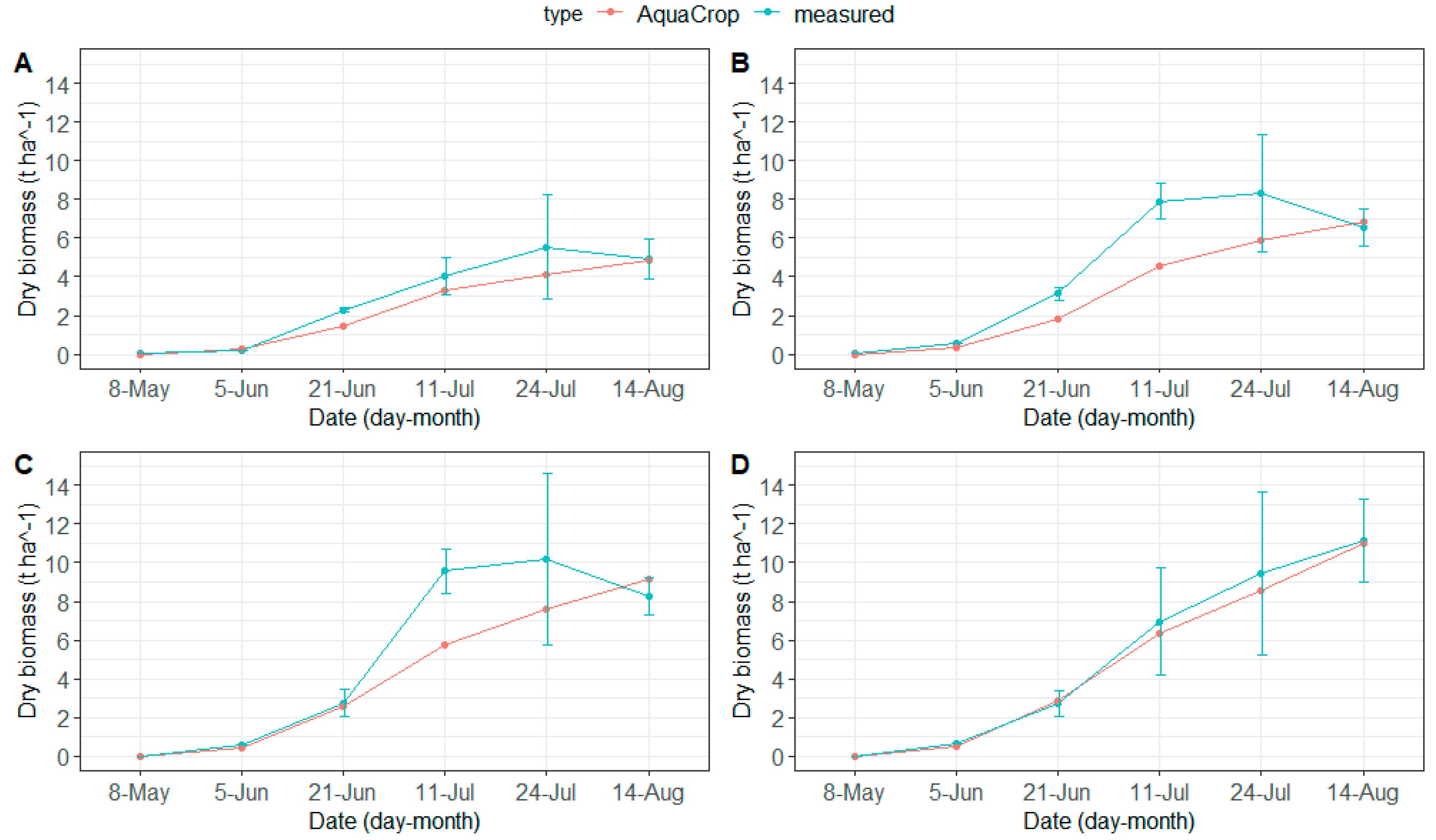
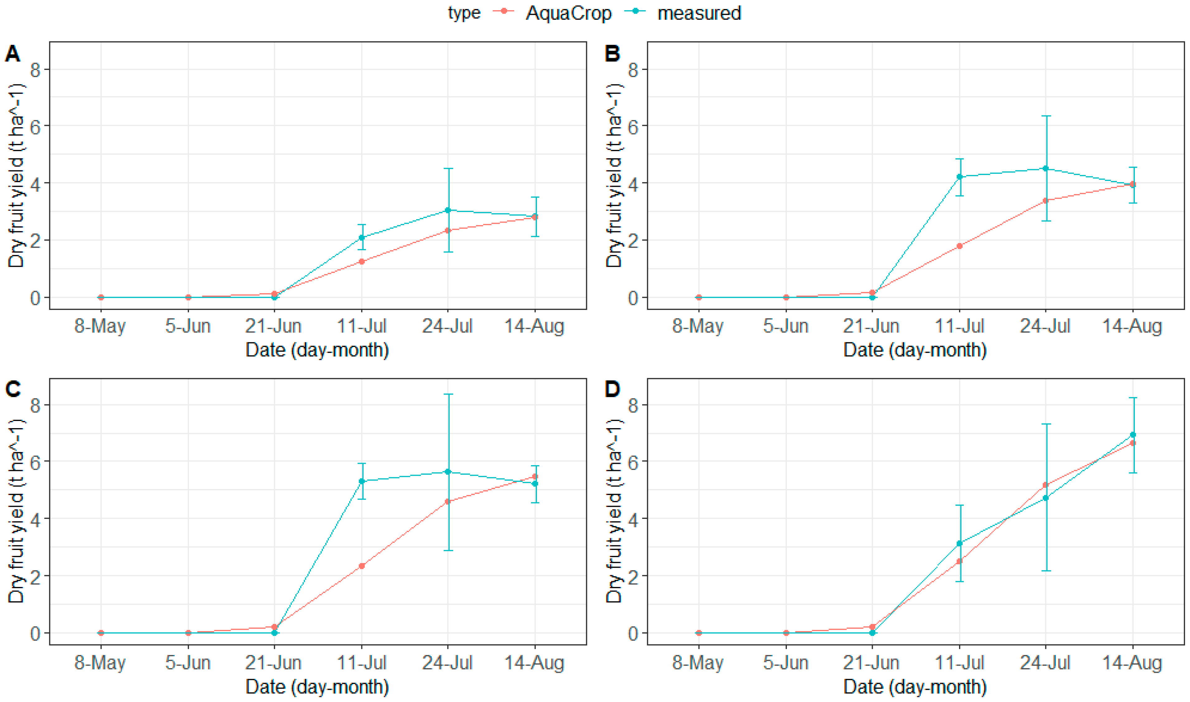
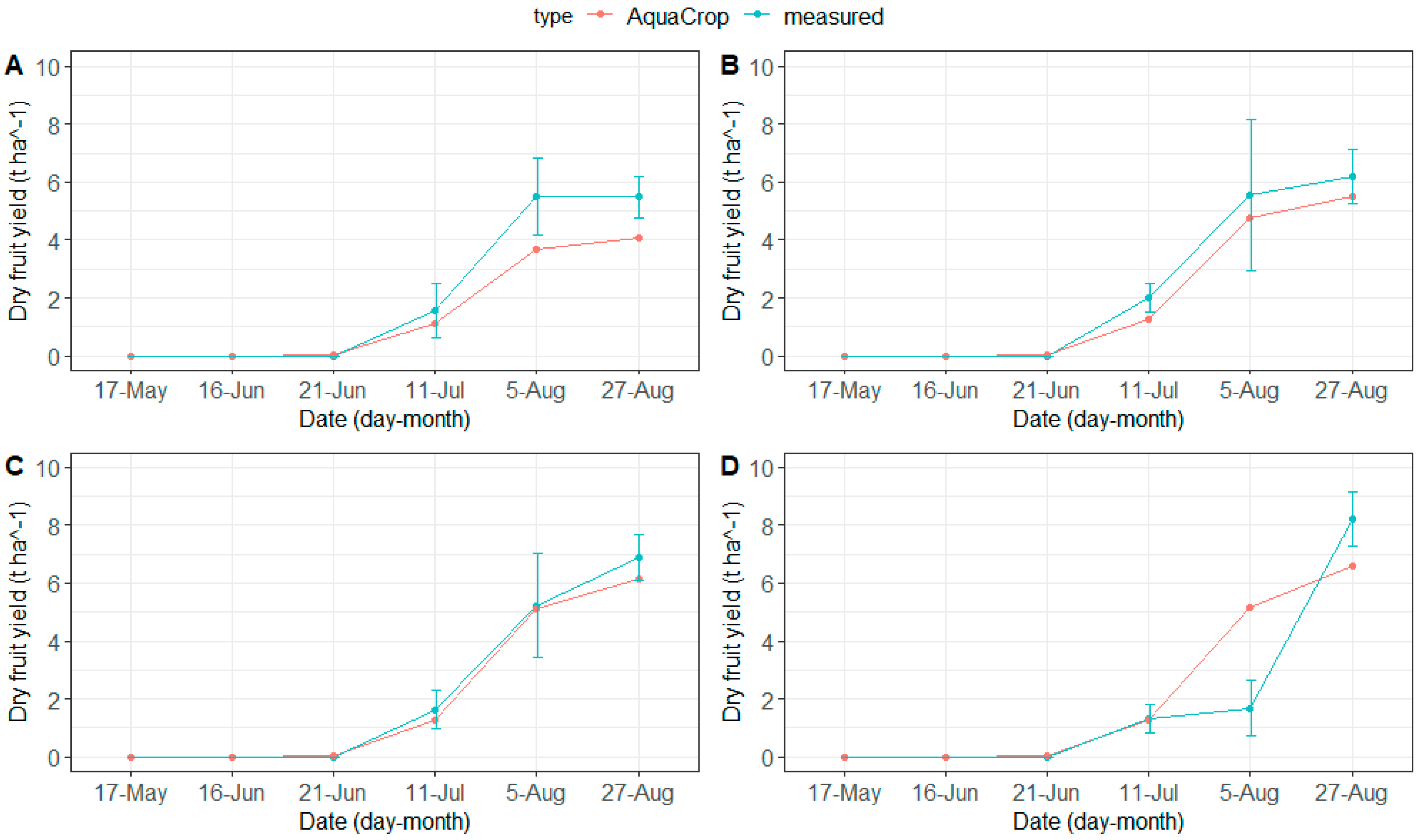
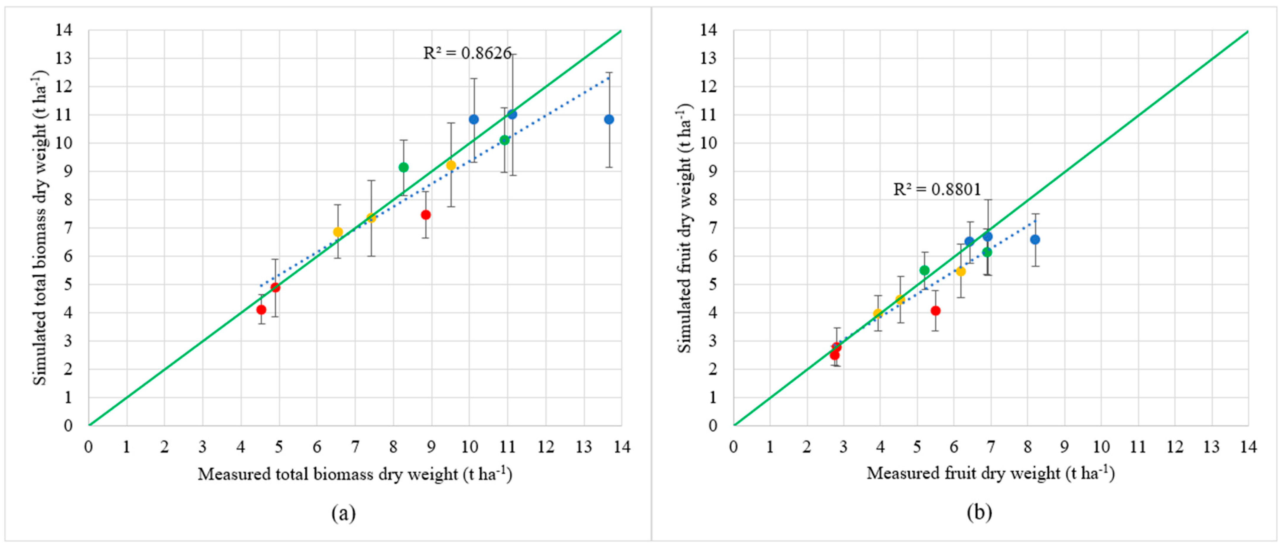
3.1. Simulation of Biomass and Yield in the Growing Season

Data from 2018 was used for the calibration of the crop file. The simulated biomass growth line of I100 showed a very good fit with the measured growth line (nRMSE = 8.66, EF = 0.99, d = 0.997) (Figure 1D). However, the simulation of biomass in the water-stressed treatments was less accurate in every case. The highest nRMSE occurred in the I50 treatment (40.54). The most accurate was the K among the water-stressed treatments (nRMSE = 26.17) (Figure 1A). Rinaldi et al. [22] presented a similar range of relative RMSE values for total dry matter (28.9–60.5%). The final biomass at harvest was very accurately estimated in every treatment (nRMSE = 6.09). The reason for the mid-season inaccuracy was that the actual biomass produced more intensive growth than estimated by AquaCrop between 21 June and 24 July, according to the samples (44–77 days after transplanting (DAT)). Nevertheless, the simulated value fell into the standard deviation of measured values at the sampling date of 24 July. Higher biomass was measured in July in all the water-stressed treatments than the final biomass at harvest, which was not as expected (Figure 1B,C). This fact implies that the sampled plants were above average by these two sampling dates. Looking at the whole growing season, the nRMSE was poor in the water stressed treatments (26.2–40.5) and very good in the case of the I100 treatment (8.7).

The yield simulation results were very similar to biomass in 2018 (Figure 2). The nRMSE showed weaker results in the case of yield, but EF and d results indicated very similar modelling accuracy to the biomass evaluation. Rinaldi et al. [22] also found weaker relative RMSE results for dry yields compared to total dry matter. The modelled fresh yield of tomato was comparable to the observed one with an error of 9% in the calibration process [37]. We found lower errors in final yields, from 1.2% to 5.5%, depending on the water supply. All the simulated results fell into the standard deviation range except for the July 11 date in the stressed treatments. Accuracy of yield at harvest date was even better than biomass estimation (nRMSE = 4.17). Still, the whole season accuracy was good only in the case of I100 (13.98) and poor (>30) in the water-stressed treatments, according to nRMSE. EF values were above the minimum (0.75), except for I50.

The simulated biomass data for 2019 gave the best result for the I75 treatment in which the nRMSE was 18.79 (Figure 3C). The inaccuracy of the data was the highest in the most stressed K treatment (nRMSE = 48.97) (Figure 3A). This low modelling performance was mostly affected by the inaccurate results related to the last sampling date before harvest on 5 August (80 DAT). It must be noted that higher biomass was found at this sampling date then at harvest. Better accuracy was reached in the I50 and I75 treatments than in 2018 (Figure 3B,C). The underestimation in the simulated values was constant in the stressed treatments and also in the I100 treatment, excluding the sampling event on 5 August. This suggests that the water productivity was higher in 2019. If underestimated values could be found only in stressed treatments, then the explanation would be the over-calibrated stress-related parameters (p). Katerji et al. [21] reported the overestimation of the model in biomass prediction under water stress, specifically after the middle of the growing season. This is contradictory of our findings that were pointing out the underestimation of AquaCrop. The modelled values at harvest were fairly accurate (nRMSE = 15.22), but significantly higher, than in the calibration year. Whole season accuracy did not reach the minimum value of EF in the case of K (EF = 0.73). A break in the growth tendency of I100 observed biomass was found at the August 5 sampling (Figure 3D).

Excessive inaccuracy occurred during the sampling dates of August in the K and I100 treatments (Figure 4A,D), resulting in extremely high nRMSE values (49 and 36.1, respectively). EF was sensitive only in the I100 treatment, where the index did not reach the threshold of acceptable accuracy (<0.75). The index of agreement (d) was less sensitive to several of these sampling dates with an inaccurate prediction. However, by the end of the growing season, the results were acceptable and underestimated in every case (nRMSE = 17.8). Since both biomass and yield were very low in I100 on 5 August, this suggests unsatisfactory plant development and the effect of overirrigation, even if there was no evidence found for this when looking at the water balance of the period 11 July–5 August. The performance of the simulation in the I50 and I75 (Figure 4B,C) was more accurate, where EF and d showed very good values (EF = 0.93–0.99 and d = ~0.99–1, respectively), but nRMSE suggested only marginal (23.24) and acceptable modelling (14.75), respectively.

Since there was no mid-season sampling in 2017, only the harvest dates could be evaluated. The results for this year are presented in

Table 6. Simulated and measured dry biomass and yield values (t ha⁻¹) for 2017 (validation) with the modelling evaluation parameters.

	Treatment	Measured	SD *	AquaCrop	Difference
Biomass	K	4.54	0.52	4.12	0.43
	I50	7.41	1.34	7.35	0.06
	I100	10.11	1.50	10.82	0.71
Yield	K	2.75	0.34	2.49	0.26
	I50	4.55	0.84	4.47	0.08
	I100	6.44	0.73	6.49	0.05
	RMSE	nRMSE	EF	d
Biomass	0.48	6.49	0.96	0.99
Yield	0.16	3.52	0.99	0.997

* SD is the standard deviation of the observed values.

. AquaCrop overestimated both biomass and yield in I100 but underestimated in the water-stressed treatments. In any case, the simulated values fell into the range of standard deviation in every case. The model evaluation values indicate an accurate simulation. Katerji et al. [21] found a weak simulation of the final yield in the severely stressed treatment. Our results justify this in 2017, where the K treatment also gave the biggest difference between the simulated and observed yield.

The most important value from a practical perspective is the harvested yield. Thus, the values at harvest are presented and evaluated for the three years (Figure 5). The nRMSE was 12.11 and 13.58 (indicating good modelling performance), EF was 0.84 and 0.81, and the d was 0.95 and 0.94 for biomass and yield, respectively. These results indicate a good simulation for biomass and yield at harvest. There were only two cases when the points were relatively far from the “perfect model line”, and even the error bars did not reach it (K and I100 in 2019). Except for these two cases, the prediction of final yield was acceptable. Thus, our results are not in agreement with the previously cited study in which only the severely stressed treatment performed a poor simulation, in the case of tomato yield [21]. In 2019, even the K treatment was not severely stressed because of the higher amount of precipitation compared to 2017 and 2018 (Table 3).

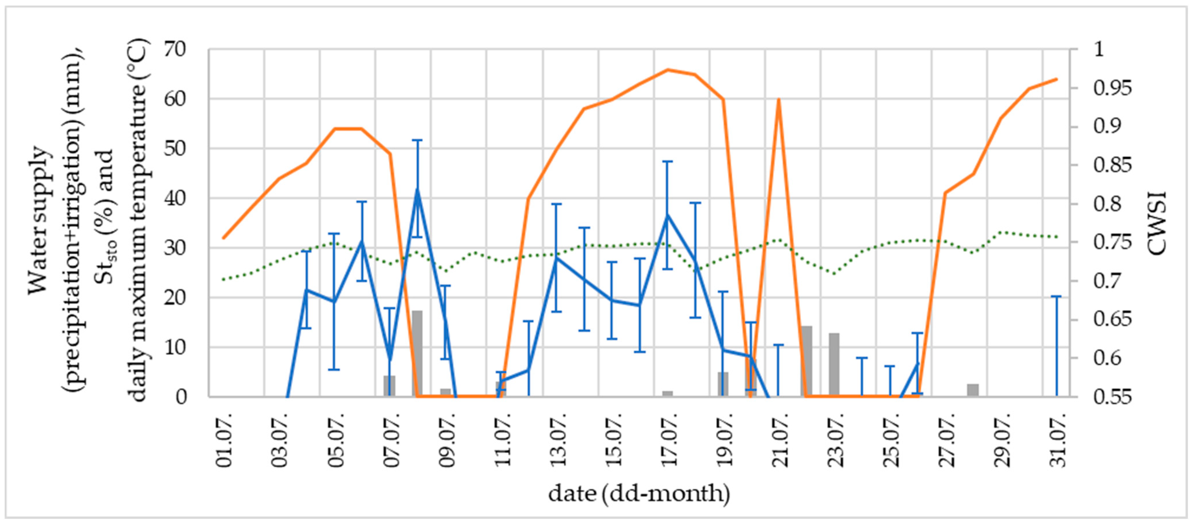
3.2. Simulation of Stomatal Closure Induced by Soil Water Stress (St_Sto)

The leaf surface temperature measurements were conducted only in July of the three years; therefore, the comparison can be done only for July. A detailed evaluation of the CWSI results is published in a previous study [15]. Even if the two indicators are not the same, both are related to water stress and range from 0 to 1 (St_Sto expressed in percentage). The St_sto is not a direct indicator of the plant water status but only refers to the relative root zone water depletion, as previously mentioned in the introduction [12].

However, due to the similarities of the simulated and measured indicators, the comparison can be conducted. However, as presented in

Table 7. Minimum and maximum values of the measured and simulated water stress-related indicators.

Water Stress-Related Indicator		2017	2018	2019
CWSI (measured)	min	0.12	0.23	0.20
	max	0.82	0.82	0.68
Ststo (modelled)	min	0	0	0
	max	48	66	74

, the range of the two indicators are different. In 2019, severe stress did not occur compared to 2018. The higher values over 50% were concentrated in the second half of July in 2019 in the K treatment, and some lower values appeared in the I50 treatment, which was not significant. An interesting observation is that the maximum CWSI reached a lower value in 2019 compared to the two other years, but the highest value of the simulated indicator was reached in this year. The measured stress values were generally lower in 2019 due to the meteorology in July, which was characterised by mild temperatures and evenly distributed rainfalls. The stress affecting the plants in 2017 was concentrated only in the second half of July. This is justified by the CWSI as well; however, there were 4 days with higher CWSI values (>0.55) when the simulated indicator remained 0. In the second half of the month, the trends of the two indicators were similar (data not shown). There were no simulated stress values higher than 0 in the I100 and only very mild stress in the I75. As a result, the comparison is not relevant in these treatments in any year, as the St_Sto was always 0.

In the I100 treatment of 2018, the highest CWSI value was 0.55. We can assume that, theoretically, stress did not develop in this treatment; thus, the values of CWSI that were indicating stress had to be over 0.55 in this case. Stress was more explicit in 2018 because of the higher temperature (mean and accumulated) compared to 2019. Thus, higher stress appeared in the K and I50 treatments. The tendencies were similar in the measured CWSI and simulated St_sto values in the K treatment of 2018, where the similarity was the best between the observed and simulated indicators (Figure 6). During the first week (55–61 DAT), both values were increasing. This can be explained by the increasing daily maximum temperature (until 5 July) and the lack of significant rainfall (until 8 July). By 8 July (62 DAT), the St_sto dropped to 0; however, CWSI reached the lowest values only two days later. The simulated value started to increase from 10 July (64 DAT) and reached the maximum value on 17 July (71 DAT), when the CWSI peaked as well. This is in agreement with the temperature data because the maximum temperature exceeded 30 °C for a four-day period before this day, and significant rainfall was absent. After this date, CWSI values were decreasing till 21 July (75 DAT). This is explained by the lower temperature on 18 July and rainfall on 19 July and 20. The simulated values followed this pattern, but in contrast with CWSI, a high value was reached on 21 July. No relevant correlation was found between CWSI and St_sto in any treatment or experimental year. The highest correlation was found in K of 2017 (0.55), but it is important to note that half of the simulated values were zero in this case.

4. Discussion

Deficit irrigation is commonly used as an irrigation water-saving strategy in the practice of processing tomato production [30]. Water use efficiency increases due to mild and moderate water stress [38], and this method also contributes to the reduction of irrigation costs [39]. Several models have been developed to help irrigation scheduling and to predict the potential biomass and fruit yield of open-field tomatoes. The Tomgro_field model was used for the evaluation of possible climatic scenarios on tomato yields. In the calibration process, the authors achieved the worst simulation results for plant dry weight in the moderately stressed and rainfed treatments, according to relative RMSE [40]. Our finding on dry biomass prediction was different in 2018 and 2019 because a better modelling performance was achieved in K and I100 treatments in 2018 and in the I50 and I75 treatments in 2019. Likewise, the same level of EF values was obtained in these cases, as found by Giuliani et al. [40]. However, in evaluating the yield results, the fresh weight of yields was evaluated in that study. Good modelling results of dry matter prediction were achieved by Giménez et al. [41] with the VegSyst model, although the goal of the study was to assess the model’s performance regarding different nitrogen supply. The EF was above 0.9, except one, which was similar to our findings in the well-irrigated treatments. Another model performance evaluation of STICS model was conducted focusing on tomato nitrogen supply. The EF and relative RMSE values indicated the lowest modelling performance for dry matter production when no additional nitrogen was supplied. The inaccuracy of the model was higher in the case of fruit dry matter in general [42]. A very strong correlation (R² = 0.99) was found between the observed and predicted yields of tomato with the SALTMED, according to the results of Alkhasha and Al-Omran [43]. The experiment contained treatments with freshwater and saline water irrigation and different types of soil amendments as well. Our prediction for harvested yields was lower (R² = 0.88). As found by a study, AquaCrop modelling combined with Sentinel-2 imagery can be used for improving the irrigation water requirements of tomatoes in the early and canopy developing stages [44].

The performance of the AquaCrop model was assessed on other horticultural crops as well. Deviations between simulated and measured yield and biomass varied on a relatively wide scale in the different water supply and plastic film mulching treatments in the case of sweet pepper. This was the consequence of different cultivars, climate, and meteorological factors, according to the authors [45]. The model was calibrated for some leafy vegetables (such as amaranth, spider flower, Swiss chard), described by high R² values. The validation gave similarly high R² for well-watered crops but performed less accurately under severe water stress conditions [46]. Minimal differences (1–2%) appeared with cabbage yield in the cross-validation process in a study [47]. Better simulation results were found for yield (nRMSE = 8.8%) than for biomass (nRMSE = 9.8%) in the case of the cowpea, which was in contradiction with our results because a lower nRMSE was found for biomass when evaluating the final yields [5]. Overestimation of bitter-gourd biomass and yield was found in a study conducted for two growing seasons [48]. Both over- and underestimation was revealed according to our findings.

5. Conclusions

AquaCrop performed quite well for the simulation of dry biomass and fruit yields at harvest time in every experimental year. However, for the evaluation of crop growth modelling, it is important to follow the simulation during the whole season. This revealed uncertainty with the modelling in several cases of both biomass and yield in the mid-season. A general underestimation of the model was found in the validation year of 2019, when samples were collected during the whole season. Only the harvested yields were evaluated in 2017, where an overestimation was found under optimal water supply and an underestimation under the stressed treatments by the validation. The simulation showed very good modelling indicator numbers for the harvested biomass and fruit yield in the non-stressed treatment in the calibration year (2018), but poor performance was found in the water-stressed treatments because of some mid-season inaccuracies. It is important to note that in the case of these inaccurate values, the measured biomass and yield in mid-season was higher than the measured value at harvest. This suggests that the sampled plants were above average. It should be noted that the model would perform differently by the evaluation of a hybrid with a longer growing season since a mid-early type hybrid was used for the calibration in this study.

No significant correlation was found between measured (CWSI) and modelled (St_Sto) water stress-related parameters in processing tomatoes, but the comparison was conducted only for one month of the growing season. However, when comparing the increasing and decreasing trends of stress, some similarities were found, especially in the treatment with severe water stress, where the most stress affected the plants. The results related to the water stress indicators may provide information to model developers to further progress the role of water stress in the modelling of plant development.

References

1. Nemeskéri, E.; Helyes, L. Physiological Responses of Selected Vegetable Crop Species to Water Stress. Agronomy 2019, 9, 447. [Google Scholar] [CrossRef] [Green Version]
2. Costa, J.M.; Ortuño, M.F.; Chaves, M.M. Deficit irrigation as a strategy to save water: Physiology and potential application to horticulture. J. Integr. Plant Biol. 2007, 49, 1421–1434. [Google Scholar] [CrossRef]
3. Koech, R.; Langat, P. Improving irrigation water use efficiency: A review of advances, challenges and opportunities in the Australian context. Water 2018, 10, 1771. [Google Scholar] [CrossRef] [Green Version]
4. Razzaghi, F.; Zhou, Z.; Andersen, M.N.; Plauborg, F. Simulation of potato yield in temperate condition by the AquaCrop model. Agric. Water Manag. 2017, 191, 113–123. [Google Scholar] [CrossRef]
5. Kanda, E.K.; Senzanje, A.; Mabhaudhi, T. Calibration and validation of the AquaCrop model for full and deficit irrigated cowpea (Vigna unguiculata (L.) Walp). Phys. Chem. Earth 2020, 124, 102941. [Google Scholar] [CrossRef]
6. Giménez, L.; Paredes, P.; Pereira, L.S. Water use and yield of soybean under various irrigation regimes and severe water stress. Application of AquaCrop and SIMDualKc models. Water 2017, 9, 393. [Google Scholar] [CrossRef]
7. Sandhu, R.; Irmak, S. Performance of AquaCrop model in simulating maize growth, yield, and evapotranspiration under rainfed, limited and full irrigation. Agric. Water Manag. 2019, 223, 105687. [Google Scholar] [CrossRef]
8. Marković, M.; Josipović, M.; Tovjanin, M.J.; Đurđević, V.; Ravlić, M.; Barač, Ž. Validating aquacrop model for rainfed and irrigated maize and soybean production in eastern croatia. Idojaras 2020, 124, 277–297. [Google Scholar] [CrossRef]
9. Hellal, F.; El-Sayed, S.; Mansour, H.; Abdel-Hady, M. Effects of micronutrient mixture foliar spraying on sunflower yield under water deficit and its evaluation by aquacrop model. Agric. Eng. Int. CIGR J. 2021, 23, 43–54. [Google Scholar]
10. Steduto, P.; Hsiao, T.C.; Raes, D.; Fereres, E. AquaCrop—The FAO Crop Model to Simulate Yield Response to Water: I. Concepts and Underlying Principles. Agron. J. 2009, 101, 426–437. [Google Scholar] [CrossRef] [Green Version]
11. Raes, D.; Steduto, P.; Hsiao, T.C.; Fereres, E. Aquacrop-The FAO Crop Model to Simulate Yield Response to Water: II. Main Algorithms and Software Description. Agron. J. 2009, 101, 438–447. [Google Scholar] [CrossRef] [Green Version]
12. Vanuytrecht, E.; Raes, D.; Steduto, P.; Hsiao, T.C.; Fereres, E.; Heng, L.K.; García-Vila, M.; Mejias Moreno, P. AquaCrop: FAO’s crop water productivity and yield response model. Environ. Model. Softw. 2014, 62, 351–360. [Google Scholar] [CrossRef]
13. Food and Agriculture Organization. FAOSTAT. Production/Yield Quantities of Tomatoes in World + (Total). Available online: http://www.fao.org/faostat/en/#data/QCL/visualize (accessed on 13 August 2021).
14. World Processing Tomato Council. WPTC World Producion Estimate of Tomatoes for Processing; General Secretary of the World Processing Tomato Council: Avignon, France, 2021. [Google Scholar]
15. Takács, S.; Pék, Z.; Csányi, D.; Daood, H.G.; Szuvandzsiev, P.; Palotás, G.; Helyes, L. Influence of water stress levels on the yield and lycopene content of tomato. Water 2020, 12, 2165. [Google Scholar] [CrossRef]
16. Bogale, A.; Nagle, M.; Latif, S.; Aguila, M.; Müller, J. Regulated deficit irrigation and partial root-zone drying irrigation impact bioactive compounds and antioxidant activity in two select tomato cultivars. Sci. Hortic. 2016, 213, 115–124. [Google Scholar] [CrossRef]
17. Giuliani, M.M.; Nardella, E.; Gagliardi, A.; Gatta, G. Deficit irrigation and partial root-zone drying techniques in processing tomato cultivated under Mediterranean climate conditions. Sustainability 2017, 9, 2197. [Google Scholar] [CrossRef] [Green Version]
18. Nemeskéri, E.; Neményi, A.; Bocs, A.; Pék, Z.; Helyes, L. Physiological factors and their relationship with the productivity of processing tomato under different water supplies. Water 2019, 11, 586. [Google Scholar] [CrossRef] [Green Version]
19. Patanè, C.; Tringali, S.; Sortino, O. Effects of deficit irrigation on biomass, yield, water productivity and fruit quality of processing tomato under semi-arid Mediterranean climate conditions. Sci. Hortic. 2011, 129, 590–596. [Google Scholar] [CrossRef]
20. Patanè, C.; Corinzia, S.A.; Testa, G.; Scordia, D.; Cosentino, S.L. Physiological and agronomic responses of processing tomatoes to deficit irrigation at critical stages in a semi-arid environment. Agronomy 2020, 10, 800. [Google Scholar] [CrossRef]
21. Katerji, N.; Campi, P.; Mastrorilli, M. Productivity, evapotranspiration, and water use efficiency of corn and tomato crops simulated by AquaCrop under contrasting water stress conditions in the Mediterranean region. Agric. Water Manag. 2013, 130, 14–26. [Google Scholar] [CrossRef]
22. Rinaldi, M.; Garofalo, P.; Rubino, P.; Steduto, P. Processing tomatoes under different irrigation regimes in Southern Italy: Agronomic and economic assessments in a simulation case study. Ital. J. Agrometeorol. 2011, 3, 39–56. [Google Scholar]
23. Linker, R.; Ioslovich, I.; Sylaios, G.; Plauborg, F.; Battilani, A. Optimal model-based deficit irrigation scheduling using AquaCrop: A simulation study with cotton, potato and tomato. Agric. Water Manag. 2016, 163, 236–243. [Google Scholar] [CrossRef]
24. Bird, D.N.; Benabdallah, S.; Gouda, N.; Hummel, F.; Koeberl, J.; La Jeunesse, I.; Meyer, S.; Prettenthaler, F.; Soddu, A.; Woess-Gallasch, S. Modelling climate change impacts on and adaptation strategies for agriculture in Sardinia and Tunisia using AquaCrop and value-at-risk. Sci. Total Environ. 2016, 543, 1019–1027. [Google Scholar] [CrossRef] [PubMed]
25. Hungarian Meteorological Service Climate of Hungary—General Characteristics. Available online: https://www.met.hu/en/eghajlat/magyarorszag_eghajlata/altalanos_eghajlati_jellemzes/altalanos_leiras/ (accessed on 5 November 2020).
26. Battilani, A.; Prieto, M.H.; Argerich, C.; Campillo, C.; Cantore, V. Tomato. In Fao Irrigation and Drainage Paper 66—Crop Yield Response to Water; Steduto, P., Hsiao, T.C., Fereres, E., Raes, D., Eds.; Food and Agriculture Organization of the United Nations: Rome, Italy, 2012; pp. 192–201. ISBN 9789251072745. [Google Scholar]
27. Allen, R.G.; Pereira, L.S.; Raes, D.; Smith, M. Crop evapotranspiration—Guidelines for computing crop water requirements. In FAO Irrigation and Drainage Paper 56; Food and Agriculture Organization of the United Nations: Rome, Italy, 1998; Volume 300, p. D05109. [Google Scholar]
28. Raes, D. AquaCrop Training Handbooks Book I Understanding AquaCrop; Food and Agriculture Organization of the United Nations: Rome, Italy, 2017; ISBN 978-92-5-109390-0. [Google Scholar]
29. Steduto, P.; Hsiao, T.C.; Fereres, E.; Raes, D. Crop Yield Response to Water; Food and Agriculture Organization of the United Nations: Rome, Italy, 2012. [Google Scholar]
30. Takács, S.; Bíró, T.; Helyes, L.; Pék, Z. Variable rate precision irrigation technology for deficit irrigation of processing tomato. Irrig. Drain. 2019, 68, 234–244. [Google Scholar] [CrossRef]
31. Macua, J.I.; Lahoz, I.; Arzoz, A.; Garnica, J. The influence of irrigation cut-off time on the yield and quality of processing tomatoes. Acta Hortic. 2003, 613, 151–153. [Google Scholar] [CrossRef]
32. Jones, H.G. Use of thermography for quantitative studies of spatial and temporal variation of stomatal conductance over leaf surfaces. Plant, Cell Environ. 1999, 22, 1043–1055. [Google Scholar] [CrossRef] [Green Version]
33. Jones, H.G.; Stoll, M.; Santos, T.; De Sousa, C.; Chaves, M.M.; Grant, O.M. Use of infrared thermography for monitoring stomatal closure in the field: Application to grapevine. J. Exp. Bot. 2002, 53, 2249–2260. [Google Scholar] [CrossRef]
34. Yang, J.M.; Yang, J.Y.; Liu, S.; Hoogenboom, G. An evaluation of the statistical methods for testing the performance of crop models with observed data. Agric. Syst. 2014, 127, 81–89. [Google Scholar] [CrossRef]
35. Nash, J.E.; Sutcliffe, J.V. River flow forecasting through conceptual models part I—A discussion of principles. J. Hydrol. 1970, 10, 282–290. [Google Scholar] [CrossRef]
36. Willmott, C.J.; Ackleson, S.G.; Davis, R.E.; Feddema, J.J.; Klink, K.M.; Legates, D.R.; O’Donnell, J.; Rowe, C.M. Statistics for the evaluation and comparison of models. J. Geophys. Res. 1985, 90, 8995–9005. [Google Scholar] [CrossRef] [Green Version]
37. Corbari, C.; Ben Charfi, I.; Mancini, M. Optimizing irrigation water use efficiency for tomato and maize fields across Italy combining remote sensing data and the aquacrop model. Hydrology 2021, 8, 39. [Google Scholar] [CrossRef]
38. Le, A.T.; Pék, Z.; Takács, S.; Neményi, A.; Helyes, L. The effect of plant growth-promoting rhizobacteria on yield, water use efficiency and Brix degree of processing tomato. Plant Soil Environ. 2018, 64, 523–529. [Google Scholar] [CrossRef] [Green Version]
39. Badr, M.A.; Abou-Hussein, S.D.; El-Tohamy, W.A. Tomato yield, nitrogen uptake and water use efficiency as affected by planting geometry and level of nitrogen in an arid region. Agric. Water Manag. 2016, 169, 90–97. [Google Scholar] [CrossRef]
40. Giuliani, M.M.; Gatta, G.; Cappelli, G.; Gagliardi, A.; Donatelli, M.; Fanchini, D.; De Nart, D.; Mongiano, G.; Bregaglio, S. Identifying the most promising agronomic adaptation strategies for the tomato growing systems in Southern Italy via simulation modeling. Eur. J. Agron. 2019, 111, 125937. [Google Scholar] [CrossRef]
41. Giménez, C.; Thompson, R.B.; Prieto, M.H.; Suárez-Rey, E.; Padilla, F.M.; Gallardo, M. Adaptation of the VegSyst model to outdoor conditions for leafy vegetables and processing tomato. Agric. Syst. 2019, 171, 51–64. [Google Scholar] [CrossRef]
42. Valdés-Gómez, H.; Gary, C.; Brisson, N.; Matus, F. Modelling indeterminate development, dry matter partitioning and the effect of nitrogen supply in tomato with the generic STICS crop-soil model. Sci. Hortic. 2014, 175, 44–56. [Google Scholar] [CrossRef]
43. Alkhasha, A.; Al-Omran, A. Simulated tomato yield, soil moisture, and salinity using fresh and saline water: Experimental and modeling study using the SALTMED model. Irrig. Sci. 2019, 37, 637–655. [Google Scholar] [CrossRef]
44. Marta, A.D.; Chirico, G.B.; Bolognesi, S.F.; Mancini, M.; D’Urso, G.; Orlandini, S.; De Michele, C.; Altobelli, F. Integrating sentinel-2 imagery with Aquacrop for dynamic assessment of tomato water requirements in southern Italy. Agronomy 2019, 9, 404. [Google Scholar] [CrossRef] [Green Version]
45. Ćosić, M.; Stričević, R.; Djurović, N.; Moravčević, D.; Pavlović, M.; Todorović, M. Predicting biomass and yield of sweet pepper grown with and without plastic film mulching under different water supply and weather conditions. Agric. Water Manag. 2017, 188, 91–100. [Google Scholar] [CrossRef]
46. Nyathi, M.K.; Van Halsema, G.E.; Annandale, J.G.; Struik, P.C. Calibration and validation of the AquaCrop model for repeatedly harvested leafy vegetables grown under different irrigation regimes. Agric. Water Manag. 2018, 208, 107–119. [Google Scholar] [CrossRef]
47. Wellens, J.; Raes, D.; Traore, F.; Denis, A.; Djaby, B.; Tychon, B. Performance assessment of the FAO AquaCrop model for irrigated cabbage on farmer plots in a semi-arid environment. Agric. Water Manag. 2013, 127, 40–47. [Google Scholar] [CrossRef]
48. Soomro, K.B.; Alaghmand, S.; Shahid, M.R.; Andriyas, S.; Talei, A. Evaluation of Aquacrop Model in Simulating Bitter Gourd Water Productivity Under Saline Irrigation. Irrig. Drain. 2020, 69, 63–73. [Google Scholar] [CrossRef]
Figure 1. Simulated and measured biomass values for the 2018 growing season (calibration). Error bars represent the standard deviation (n = 4). The (AD) letters refer to the K, I50, I75, and I100 treatments, respectively.
Water 13 03587 g001
Figure 2. Simulated and measured yield values for the 2018 growing season (calibration). Error bars represent the standard deviation (n = 4). The (AD) letters refer to the K, I50, I75, and I100 treatments, respectively.
Water 13 03587 g002
Figure 3. Simulated and measured biomass values for the 2019 growing season (validation). Error bars represent the standard deviation (n = 4). The (AD) letters refer to the K, I50, I75, and I100 treatments, respectively.
Water 13 03587 g003
Figure 4. Simulated and measured yield values for the 2019 growing season (validation). Error bars represent the standard deviation (n = 4). The (AD) letters refer to the K, I50, I75, and I100 treatments, respectively.
Water 13 03587 g004
Figure 5. Simulated and measured values at harvest for (a) biomass and (b) yield. Error bars represent the standard deviation. Solid green lines represents the perfect model, and the dotted line represents the fitted linear model (n = 11). Dot colors indicate: red (K), yellow (I50), green (I75), and blue (I100).
Water 13 03587 g005
Figure 6. Comparison of water stress-related, simulated Ststo (percent water stress inducing stomatal closure–AquaCrop) (orange), and measured CWSI values (blue) in the treatment with severe stress. Error bars represent the standard error of CWSI values. Grey columns refer to the irrigation and rainfall events (mm) and green dotted line refers to the daily maximum temperature.
Water 13 03587 g006