Three-Parameter Regulation Rules for the Long-Term Optimal Scheduling of Multiyear Regulating Storage Reservoirs

Abstract

The perennial storage water level (PL), the water level at the end of wet season (WL), and the water level at the end of dry season (DL) are three critical water levels for multiyear regulating storage (MRS) reservoirs. Nevertheless, the three critical water levels have not been paid enough attention, and there is no general method that calculates them in light of developing regulating rules for MRS reservoirs. In order to address the issue, three-parameter regulation (TPR) rules based on the coordination between the intra- and interannual regulation effects of MRS reservoirs are presented. Specifically, a long-term optimal scheduling (LTOS) model is built for maximizing the multiyear average hydropower output (MAHO) of a multireservoir system. The TPR rules are a linear form of rule with three regulation parameters (annual, storage, and release regulation parameters), and use the cuckoo search (CS) algorithm to solve the LTOS model with three regulation parameters as the decision variables. The approach of utilizing the CS algorithm to solve the LTOS model with the WL and DL as the decision variables is abbreviated as the OPT approach. Moreover, the multiple linear regression (MLR) rules and the artificial neural network (ANN) rules are derived from the OPT approach-based water-level processes. The multireservoir system at the upstream of Yellow River (UYR) with two MRS reservoirs, Longyangxia (Long) and Liujiaxia (Liu) reservoirs, is taken as a case study, where the TPR rules are compared with the OPT approach, the MLR rules, and the ANN rules. The results show that for the UYR multireservoir system, (1) the TPR rules-based MAHO is about 0.3% (0.93 × 10⁸ kW∙h) more than the OPT approach-based MAHO under the historical inflow condition, and the elapsed time of the TPR rules is only half of that of the OPT approach; (2) the TPR rules-based MAHO is about 0.79 × 10⁸ kW∙h more than the MLR/ANN rules-based MAHO under the historical inflow condition, and the TPR rules can realize 0.1–0.4% MAHO more than the MLR and ANN rules when the reservoir inflow increases or reduces by 10%. According to the annual regulation parameter, the PLs of Long and Liu reservoirs are 2572.3 m and 1695.2 m, respectively. Therefore, the TPR rules are an easy-to-obtain and adaptable LTOS rule, which could reasonably and efficiently to determine the three critical water levels for MRS reservoirs.

1. Introduction

As reservoirs are one of the most effective engineering measures for regulating and utilizing river runoff, many countries have built large numbers of reservoirs along big rivers and formed a variety of multireservoir systems [1,2,3,4]. A multireservoir system generally has one or more MRS reservoirs, which play the most important roles in the system for their large storage capabilities [5,6]. Specifically, the MRS reservoirs are not only able to reserve abundant water in a wet season to meet water demands in a dry season (i.e., the intraannual regulation effect), but could also store rich water in a wet year to compensate water shortages in a dry year (i.e., the interannual regulation effect) [7,8,9]. Moreover, an MRS reservoir could control the inflow processes of smaller reservoirs downstream and alter the flow regime of the river on which it is built to a considerable extent [5,7,9,10].

According to the scheduling timescale, reservoir scheduling could be generally divided into short-term (hourly/daily) scheduling, mid-term (weekly/monthly) scheduling, and long-term (seasonal/annual) scheduling [11,12]. The LTOS of MRS reservoirs could offer water utilization objectives and constraints for the short- and mid-term scheduling of a multireservoir system, hence influencing the comprehensive water utilization benefits of the entire system [10,13]. In the LTOS, there are three critical water levels for an MRS reservoir, namely, the PL, the WL, and the DL. Specifically, the PL divides the active storage space into the annual and perennial storage spaces, where the stored water volumes are utilized for intra- and interannual regulation effects, respectively [11,13,14,15]. In addition, the larger the size of the perennial storage space, the stronger the interannual regulation effect. The WL not only determines the WSV at the end of a wet season, but also affects the available water (storage and inflow) volume during the dry season of the same year [16,17]. As for the DL, it not only influences the discharge during the dry season of a year, but also affects the available water volume of the next year [5,7,12,18].

The three critical water levels of MRS reservoirs are of important significance to the LTOS of a multireservoir system. However, to our knowledge, studies on the three critical water levels are less common in the available literature, especially the PL and the WL. The exiting relevant literature also failed to provide a general method to determine the three critical water levels of MRS reservoirs. For example, Draper and Lund [14] did not directly investigate the PL, but theoretically analyzed the optimal carryover storage value function for a reservoir. Nevertheless, they pointed out that their findings would face additional challenges in the LTOS of a multireservoir system. In order to alleviate the conflict between flood control and water utilization in wet season, Chou and Wu [19] investigated the stagewise flood moderating rules, and Peng et al. [20] and Liu et al. [21] studied the dynamic control of flood limit level of reservoirs, but they failed to specify how much water should be retained in MRS reservoirs at the end of the wet season. Some scholars are devoted to determining the DL by means of statistical regression analysis methods or machine learning techniques [11,12,15,19,22]. However, these studies focused on determining the DL for an individual MRS reservoir without considering its role in a multireservoir system, or they treated the DL of each year in isolation without considering the linkage of DL between adjacent years.

Implicit stochastic optimization is often used to derive the optimal reservoir scheduling rules because it enables most characteristics of stochastic reservoir inflows and is more operational than explicit stochastic optimization [4,23]. Within the framework of an implicit stochastic optimization, the optimal scheduling rules could be derived by two approaches when the form of scheduling rules is predetermined [1,22,23]. One is the indirect derivation approach that deduces the parameters of the predetermined rules by fitting the optimal scheduling process. Another is the direct derivation approach which directly determines the parameters of the predetermined rules by optimizing scheduling objectives. Both approaches have to face the problem of selecting the form of scheduling rules. Currently, the available forms of scheduling rules include linear or nonlinear regression methods, decision trees, artificial neural networks, support vector machines, and so on [5,23,24,25,26]. These forms of rules are often derived by the indirect derivation approach, which is less efficient than the direct derivation approach [23]. Moreover, these forms of rules are always complex, especially the nonlinear rules. A more complex form of rules usually means that there are more parameters to be calibrated under given input variables, which could achieve better scheduling objectives but at a higher computational cost [27,28]. To make matters more troublesome, these forms of rules could determine the WL and the DL for an MRS reservoir but cannot determine the PL, because it is not intuitively reflected in the optimal water-level process.

In summary, the core problem of the study is the question of how to reasonably and effectively determine the PL, WL, and DL. To this end, TPR rules are proposed for MRS reservoirs in the LTOS. Based on the coordination between the intra- and interannual regulation effects, a linear form of TPR rules is derived by the direct derivation approach. Taking the multireservoir system at the UYR as a case study, the application effects of TPR rules would be verified. Therefore, the rest of the paper is organized as follows. Section 2 describes the LTOS model, the CS algorithm, the MLR, ANN, and TPR rules, and the other methods. Then, Section 3 introduces the multireservoir system at the UYR and the data employed in the study. Section 4 shows the application results of the MLR, ANN, and TPR rules. Moreover, the results are discussed in Section 5. Finally, the conclusions are drawn in Section 6.

2. Methods

2.1. Derivation of LTOS Rules for MRS Reservoirs

2.1.1. LTOS Model and CS Algorithm

Hydropower production is an important function of many multireservoir systems [3,12,29]. The LTOS model of hydropower generation for a multireservoir system built by Liu et al. [26] is employed in the study. In the LTOS, a hydrological year is separated into a wet season and a dry season, which are the calculation intervals. Specifically, the objective function and constraints of the LTOS model are described as follows.

(1) Objective function

The MAHO is a key benefit index of multireservoir systems [3,26,30]. The objective function of the LTOS model, expressed by Equation (1), is to maximize the MAHO.

$$\mathrm{Max} E=\frac{24}{N}{\displaystyle \sum _{i=1}^N{\displaystyle \sum _{k=1}^m\left[T_{\mathrm{W}}{N}_{\mathrm{W},k,i}+T_{\mathrm{D}}{N}_{\mathrm{D},k,i}\right]}}$$

(1)

where E denotes the MAHO of a multireservoir system; n is the number of years in the whole scheduling period; i is the serial number of a year; m is the number of hydropower reservoirs in a multireservoir system; k represents the serial number of a reservoir; T_W and T_D represent the numbers of days in wet and dry seasons, respectively, unit: D; and N_W,k,i and N_D,k,i denote the average power generations of the kth reservoir during wet and dry seasons of the ith year, respectively, unit: kW.

The N_W,k,i and N_D,k,i in Equation (1) are calculated by

$$\{\begin{array}{l}{N}_{\mathrm{W},k,i}={\mathrm{F}}_{\mathrm{W},k}\left(Z_{\mathrm{D},k,i-1},Z_{\mathrm{W},k,i}\right)\\ N_{\mathrm{D},k,i}={\mathrm{F}}_{\mathrm{D},k}\left(Z_{\mathrm{W},k,i},Z_{\mathrm{D},k,i}\right)\end{array}$$

(2)

where f_W,k() and f_D,k() represent the power generation formulas of the kth reservoir during wet and dry seasons, respectively; Z_D,k,i−1 denotes the water level of the kth reservoir at the end of the dry season of the (i − 1)th year, unit: m; and Z_W,k,i and Z_D,k,i are the water levels of the kth reservoir at the ends of wet and dry seasons of the ith year, respectively, unit: m.

For run-of-river hydropower reservoirs in the multireservoir system, it is noted that the design water heads, rather than the water levels, are considered in calculating the average power generations during the wet and dry seasons.

(2) Constraints

(a) Water balance equations

$$\{\begin{array}{l}{S}_{\mathrm{W},k,i}=S_{\mathrm{D},k,i-1}+I_{\mathrm{W},k,i}-O_{\mathrm{W},k,i}-L_{\mathrm{W},k,i}\\ S_{\mathrm{D},k,i}=S_{\mathrm{W},k,i}+I_{\mathrm{D},k,i}-O_{\mathrm{D},k,i}-L_{\mathrm{D},k,i}\end{array}$$

(3)

where S_W,k,i and S_D,k,i are the WSVs of the kth reservoir at the ends of the wet and dry seasons of the ith year, respectively, unit: m³; S_D,k,i-1 denotes the WSV of the kth reservoir at the end of the dry season of the (i − 1)th year, unit: m³; I_W,k,i and I_D,k,i are the inflow volumes of the kth reservoir during the wet and dry seasons of the ith year, respectively, unit: m³; O_W,k,i and O_D,k,i represent the outflow volumes of the kth reservoir during the wet and dry seasons of the ith year, respectively, unit: m³; and L_W,k,i and L_D,k,i denote the water loss (evaporation and leakage) volumes of the kth reservoir during the wet and dry seasons of the ith year, respectively, unit: m³.

(b) Water-level constraints

$$\{\begin{array}{l}{Z}_k^{\mathrm{D}}\le Z_{\mathrm{D},k,i-1},Z_{\mathrm{D},k,i-1}\le \min \left(Z_{\mathrm{W},k,i},Z_k^{\mathrm{F}}\right)\\ Z_{\mathrm{W},k,i}\le Z_k^{\mathrm{N}}\end{array}$$

(4)

where Z^D_k, Z^F_k, and Z^N_k denote the dead water level, the flood limit water level, and normal water level of the kth reservoir, respectively, unit: m.

(c) Outflow constraints

$$O_{\min ,k}\le O_{\mathrm{D},k,i}\le O_{\mathrm{W},k,i}\le O_{\max ,k}$$

(5)

where O_min,k and O_max,k represent the minimum and maximum allowable outflow volumes of the kth reservoir, respectively, unit: m³.

(d) Power generation constraints

$$N_{\min ,k}\le N_{\mathrm{W},k,i},N_{\mathrm{D},k,i}\le N_{\max ,k}$$

(6)

where N_min,k and N_max,k denote the minimum and maximum allowable power generations of the kth reservoir, respectively, unit: kW.

(e) Initial conditions

$$Z_{\mathrm{D},k,0}=Z_k^{\mathrm{D}}$$

(7)

where Z_D,k,0 is the initial water level (water level at the beginning of the first year) of the kth reservoir, unit: m.

The evolutionary and metaheuristic algorithms are the most popular approaches to resolve the high-dimensional, nonlinear, and multistage optimization operation problems of multireservoir systems [3,29,31,32]. The CS algorithm is an evolutionary and metaheuristic algorithm with high search performance, few parameters, and strong robustness, and has achieved good results in solving complex reservoir scheduling problems in recent years [26,33,34]. In the study, the CS algorithm is utilized to resolve the LTOS model. More details about the CS algorithm can be found in Ming et al. [33] and Meng et al. [34].

2.1.2. Formulation of LTOS Rules

For any LTOS rules, determining the input variables and the parameters is a key problem. In actuality, there are many factors influencing the WL and the DL of MRS reservoirs. The WSV at the beginning of a wet/dry season and the inflow during the wet/dry season are two important and commonly used input variables to determine the WL/DL [11,14,15,19,26]. Therefore, the two factors are also used as the input variables of the MLR, ANN, and TPR rules. In addition, the WSVs at the ends of wet and dry seasons are determined according to the three LTOS rules, and then the corresponding WL and DL are calculated based on the elevation-storage relationship of an MRS reservoir.

For convenience, the approach of utilizing the CS algorithm to solve the LTOS model with the water levels (the WL and DL) as the decision variables is abbreviated as the OPT approach. The MLR and ANN rules are derived from the OPT approach-based water-level processes.

(1) MLR and ANN rules

The MLR rules are a classical linear LTOS rule with the following equations.

$$\{\begin{array}{l}{S}_{\mathrm{W},i,k}={\mathrm{A}}_{\mathrm{W},1}{O}_{\mathrm{W},i,k}^{\mathrm{Up}}+{\mathrm{A}}_{\mathrm{W},2}{I}_{\mathrm{W},i,k}^{\mathrm{Loc}}+{\mathrm{A}}_{\mathrm{W},3}{S}_{\mathrm{D},i-1,k}+c_{\mathrm{W}}\\ S_{\mathrm{D},i,k}={\mathrm{A}}_{\mathrm{D},1}{O}_{\mathrm{D},i,k}^{\mathrm{Up}}+{\mathrm{A}}_{\mathrm{D},2}{I}_{\mathrm{D},i,k}^{\mathrm{Loc}}+{\mathrm{A}}_{\mathrm{D},3}{S}_{\mathrm{W},i,k}+c_{\mathrm{D}}\end{array}$$

(8)

where S_W,i,k and S_D,i,k separately denote the WSVs of the kth reservoir at the ends of wet and dry seasons of the ith year, unit: m³; S_D,i−1,k is the WSV of the kth reservoir at the end of dry season of the (i − 1)th year, unit: m³; $O_{\mathrm{W},i,k}^{\mathrm{Up}}$ and $O_{\mathrm{D},i,k}^{\mathrm{Up}}$ represent the total outflow volumes of the upstream reservoirs flowing into the kth reservoir during wet and dry seasons of the ith year, respectively, unit: m³; $I_{\mathrm{W},i,k}^{\mathrm{Loc}}$ and $I_{\mathrm{D},i,k}^{\mathrm{Loc}}$ denote the local inflow volumes between the upstream reservoirs and the kth reservoir during wet and dry seasons of the ith year, respectively, unit: m³; a_W,j and a_D,j (j = 1 − 3) are the regression coefficients of MLR rules in wet and dry seasons, respectively; c_W and c_D are the constant terms of MLR rules in wet and dry seasons, respectively.

The FFNN is commonly used to derive the ANN rules in many studies for its good performances in long-term scheduling of reservoirs [25,26]. In the study, a two-layer FFNN with a hidden layer and an output layer is employed to formulate the ANN rules.

The expressions of the ANN rules are described as follows.

$$\{\begin{array}{l}{S}_{\mathrm{W},i,k}=\mathrm{N}e{\mathrm{t}}_{\mathrm{W},k}\left[O_{\mathrm{W},i,k}^{\mathrm{Up}},I_{\mathrm{W},i,k}^{\mathrm{Loc}},S_{\mathrm{D},i-1,k}\right]\\ S_{\mathrm{D},i,k}=\mathrm{N}e{\mathrm{t}}_{\mathrm{D},k}\left[O_{\mathrm{D},i,k}^{\mathrm{Up}},I_{\mathrm{D},i,k}^{\mathrm{Loc}},S_{\mathrm{W},i,k}\right]\end{array}$$

(9)

where Net_W,k and Net_D,k represent the trained FFNNs for the kth reservoir during wet and dry seasons, respectively.

(2) TPR rules

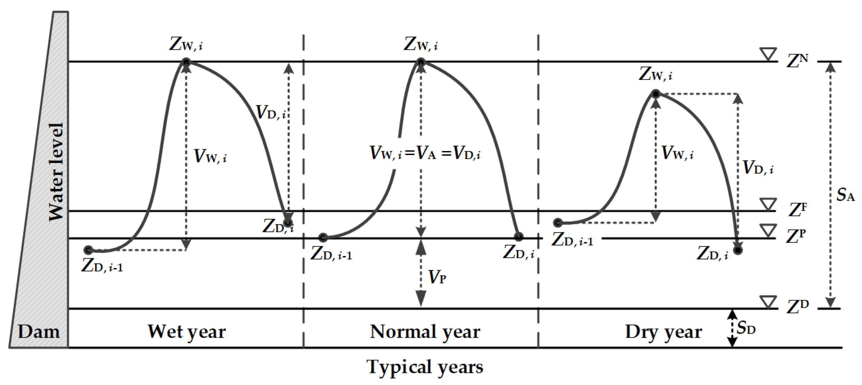
The PL, WL, and DL of an MRS reservoir for three typical years (a wet year, a normal year, and a dry year) are shown in Figure 1. It can be seen that the PL divides the active storage space (S_A) into the annual storage space (V_A) and the perennial storage space (V_P), and the relative elevations between the WL and the DL are different for three typical years.

For an MRS reservoir, the V_A and V_P usually increase with the S_A, and the intra- and interannual regulation capacity of the reservoir becomes stronger accordingly. Thus, more water could be stored in a wet year (wet season), more water could be released in a dry year (dry season), and a balance between water storage in a wet season and water release in a dry season could be maintained in a normal year. Moreover, the more the inflow volume in a wet season, the more water stored in the reservoir during a wet season. The less the inflow volume in a dry season, the more water releases from the reservoir during a dry season. Therefore, as shown in Figure 1, the V_W,_i is more than the V_D,i, and the Z_D,i is higher than the Z_D,i−1 when the ith year is a wet year. In contrast, V_W,_i is less than V_D,i and Z_D,i is lower than Z_D,i−1 if the ith year is a dry year. When the ith year is a normal year, V_W,_i is equal to V_D,i, Z_D,i is equal to Z_D,i−1, and V_W,i (V_D,i) is also equal to V_A. Moreover, V_W,_i in a wet year (say the ith year) is more than V_W,_j in a normal year (say the jth year), and V_W,_j is also larger than V_W,_k in a dry year (say the kth year); and V_D,_i is less than V_D,_j, and V_D,_j is also smaller than V_D,_k.

According to the above understanding on the coordination between the intra- and interannual regulation effects, an additional condition could be set for the LTOS model of MRS reservoirs, which is formulated as follows.

$$\{\begin{array}{l}{V}_{\mathrm{A},k}=\phi \cdot S_{\mathrm{A},k}\\ V_{\mathrm{W},i,k}-V_{\mathrm{A},k}=\lambda \cdot \left(I_{\mathrm{W},i,k}-I_{\mathrm{W},k}^{*}\right)\\ V_{\mathrm{A},k}-V_{\mathrm{D},i,k}=\mu \cdot \left(I_{\mathrm{D},i,k}-I_{\mathrm{D},k}^{*}\right)\end{array}$$

(10)

where V_A,k and S_A,k denote the annual and active storage spaces of the kth reservoir, respectively, unit: m³; V_W,i,k and V_D,i,k are the increased and reduced WSVs of the kth reservoir during wet and dry seasons of the ith year, respectively, unit: m³; I_W,i,k and I_D,i,k are the natural inflow volumes of the kth reservoir in wet and dry seasons of the ith year, respectively, unit: m³; I^*_W,k and I^*_D,k represent the multiyear average natural inflow volumes of the kth reservoir in wet and dry seasons, respectively, unit: m³; and φ, λ, and μ denote the annual, storage, and release regulation parameters, respectively.

From Equation (10), it could be seen that the three regulation parameters are dimensionless. The V_A is not more than the S_A, and thus the value range of φ is [0, 1]. In Equation (10), (V_W,i,k − V_A,k) and (V_A,k − V_D,i,k) are collectively referred to as the seasonal storage anomaly of the kth reservoir, and (I_W,i,k − I^*_W,k) and (I_D,i,k − I^*_D,k) are collectively referred to as the seasonal inflow anomaly of the kth reservoir. Generally, the seasonal storage anomaly is not more than the seasonal inflow anomaly for an MRS reservoir, and thus the value ranges of λ and μ are [0, 1].

The three parameters in Equation (10) together control the annual storage space, the increased WSV in a wet season, and the reduced WSV in a dry season. Further, the φ determines the PL of an MRS reservoir, and reflects the allocation of active storage space for intra- and interannual regulation effects. The λ and the μ describe the storage–release flexibilities of an MRS reservoir in wet and dry seasons, respectively. For an MRS reservoir, as the φ increases, the PL is lower, and the interannual regulation capability becomes weaker. The larger the λ and μ, the more pronounced the regulation of seasonal inflows by MRS reservoirs, and the bigger the differences in the WL/DL between years.

According to Equation (10), the TPR rules are formulated as follows.

$$\{\begin{array}{l}{S}_{\mathrm{W},i,k}=\lambda \cdot I_{\mathrm{W},i,k}+S_{\mathrm{D},i-1,k}+\phi \cdot S_{\mathrm{A},k}-\lambda \cdot I_{\mathrm{W},k}^{*}\\ S_{\mathrm{D},i,k}=\mu \cdot I_{\mathrm{D},i,k}+S_{\mathrm{W},i,k}-\phi \cdot S_{\mathrm{A},k}-\mu \cdot I_{\mathrm{D},k}^{*}\end{array}$$

(11)

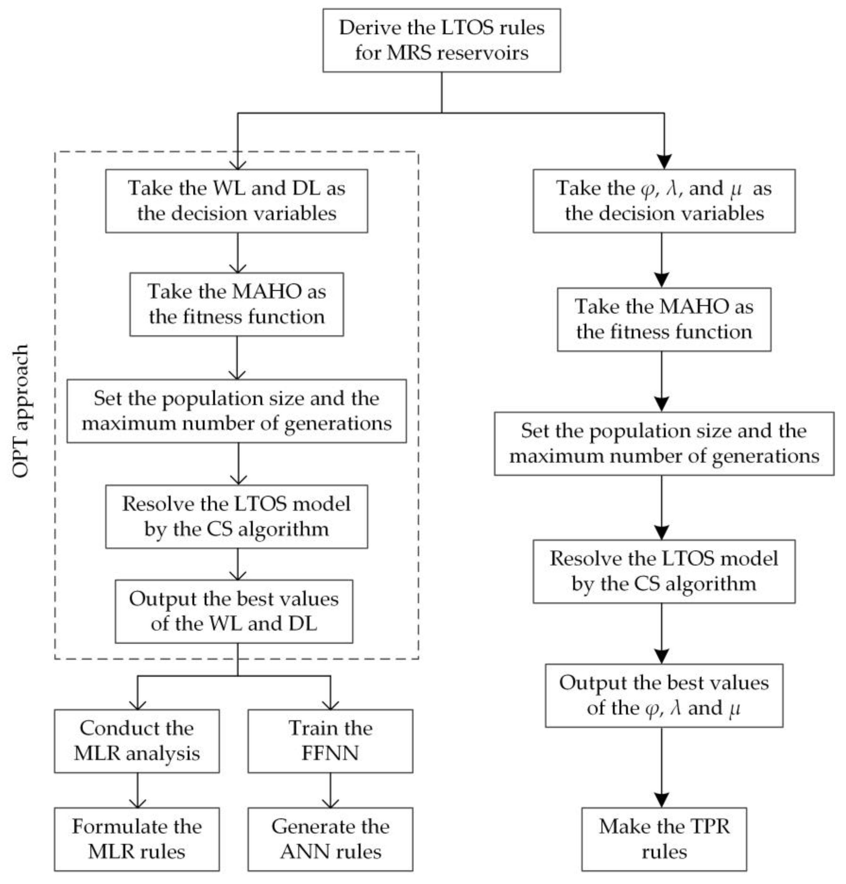
The flow chart of deriving the MLR, ANN, and TPR rules is shown in Figure 2.

2.2. Randomness and Correlation Tests

Being subject to finite iterations, the water-level processes of MRS reservoirs solved by the evolutionary and metaheuristic algorithms may show some randomness which pose a challenge to formulate the LTOS rules. Therefore, it is necessary to test the randomness of the water-level processes.

The Ljung-Box test method performs well in randomness test of a time series [35]. The Ljung-Box test statistic (Q_LB) is built as follows.

$$Q_{\mathrm{LB}}=T\cdot \left(T+2\right)\cdot {\displaystyle \sum _{i=1}^l\frac{r_i^2}{T-i}}$$

(12)

where T is the length of a given time series; l (l ≥ 1) is the maximum time lag which is not more than n^0.5; and r_i is the autocorrelation coefficient of the time series with the time lag i.

Generally, the smaller the Q_LB, the stronger the randomness of the time series. The Q_LB obeys χ² distribution with the freedom degree l when T is larger than 20. Under the significance level α, a time series is nonrandom if Q_LB > χ²_1−α(l), where χ²_1−α(l) denotes the 1−α fractile of the χ² distribution with the freedom degree l; otherwise, the time series is random.

The MLR and ANN rules are derived by fitting the optimal water-level processes of MRS reservoirs. Thus, it is also necessary to investigate the fitting effects of the MLR and ANN rules. The fitting effect of LTOS rules is measured by the Pearson correlation coefficient (R) between the optimal and simulated water-level processes. The bigger the R value, the better the fitting effect. The t test statistic [36] for testing the significance of the R is expressed as follows.

$$t=\sqrt{\left(T-2\right)\frac{R^2}{1-R^2}}$$

(13)

where t is the t test statistic that follows the t distribution with the freedom degree T − 2.

Under the significance level α, the R is significant if t > t_1−α/2(T − 2), where t_1−α/2(T − 2) denotes the 1 − α/2 fractile of the t distribution with the freedom degree (T − 2); otherwise, the R is insignificant.

2.3. Sensitivity Analysis

Sensitivity analysis reveals the sensitivity of a model or an equation-based rule to input variables or parameters [37]. Reservoir inflows have significant impacts on the LTOS of multireservoir system [26]. Under climate change and human activities, the flow regimes of many rivers have changes to different degrees which pose big challenges to the LTOS of multireservoir systems [6,26]. In order to analyze the sensitiveness of the three forms of LTOS rules (TPR, MLR, and ANN) to reservoir inflows, the reservoir inflow process at each dam site is increased (reduced) by 10% based on the historical runoff process.

For convenience, the condition that the inflow process is increased (reduced) by 10% for each reservoir is referred to as the increased inflow condition (reduced inflow condition). If LTOS rules-based MAHO of the multireservoir system significantly exceeds (reduces) by more than 10% under the increased/reduced inflow condition, the LTOS rules are very sensitive to the reservoir inflow variations. When the MAHO increases/reduces by about 10% under the two conditions, the LTOS rules are sensitive to the inflow variations. If the MAHO increases/reduces by less than 10% obviously, the LTOS rules are not sensitive to the inflow variations.

3. Study Area and Data

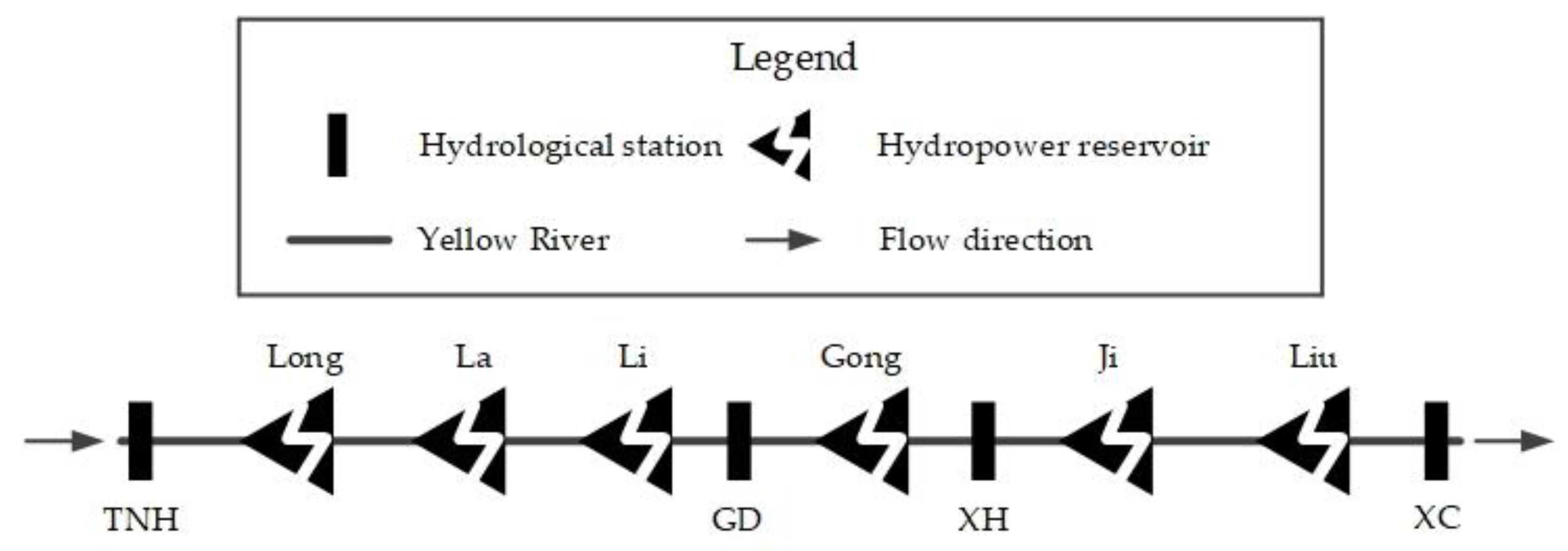
With high altitude, rich water resources, and good hydropower development conditions, the UYR has been recognized as one of the eight key hydropower bases in China [38]. At the UYR, Long, La, Li, Gong, Ji, and Liu are six important cascade hydropower reservoirs with an installed capacity of more than one million kilowatts. Long and Liu are the two largest reservoirs in the six reservoirs. Moreover, there are four typical hydrological stations at the UYR, i.e., TNH, GD, XH, and XC. The relative locations of hydropower reservoirs and hydrological stations at the UYR and the characteristic water levels of Long and Liu reservoirs are shown in Figure 3 and

Table 1. Characteristic water levels of Long and Liu reservoirs.

Reservoir	Dead Water Level (m)	Flood Limit Water Level (m)	Normal Water Level (m)
Long	2530	2594	2600
Liu	1694	1726	1735

, respectively.

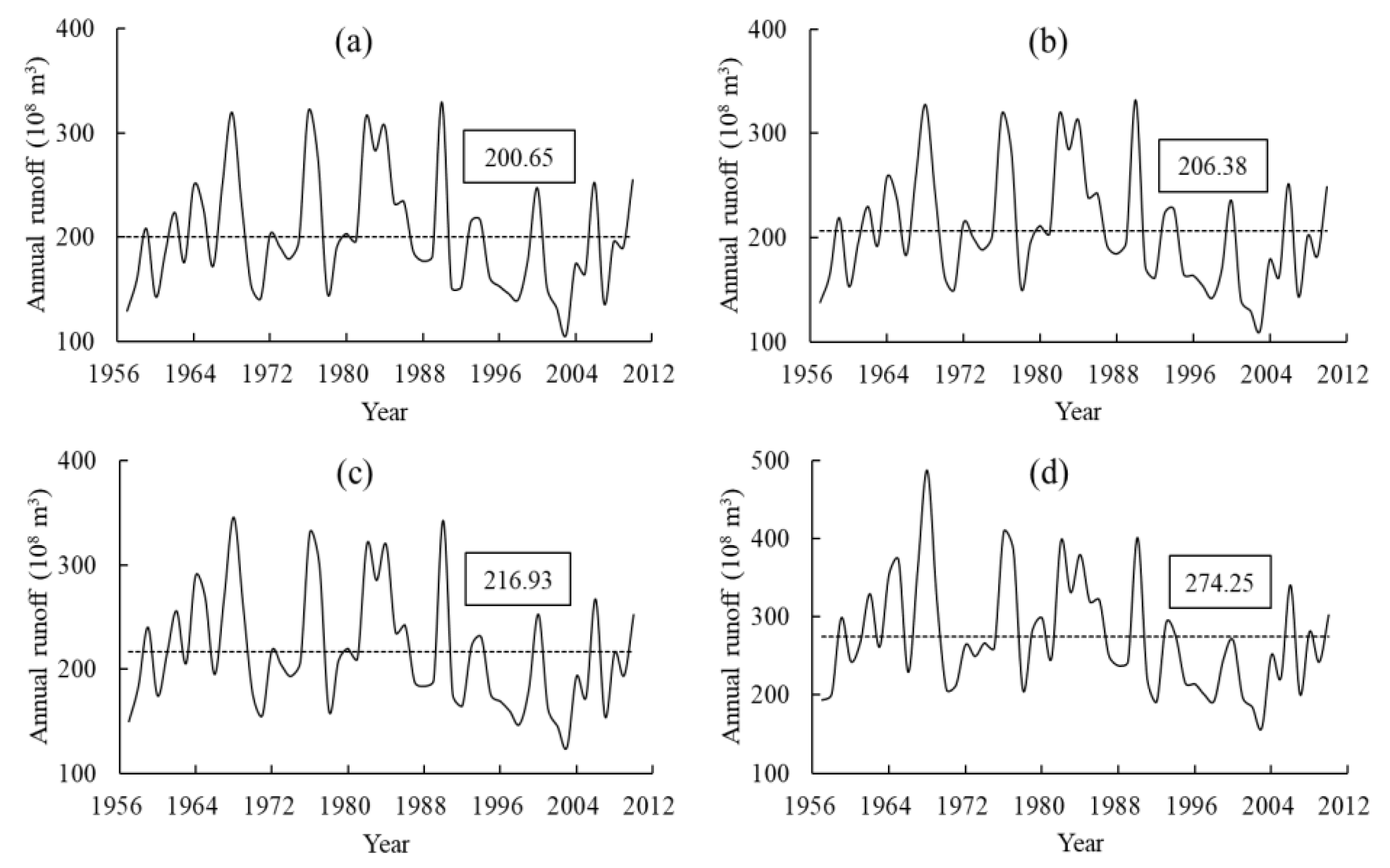
The UYR multireservoir system, which is composed of Long, La, Li, Gong, Ji, and Liu reservoirs, is taken as the case study. The hydrologic year of the UYR is from the beginning of June to the end of May, including a wet season (June–October) and a dry season (November–May). The monthly runoff data (June 1956–May 2010, total of 54 years) of TNH, GD, XH, and XC stations were collected from the hydrological yearbooks of the Yellow River basin. The annual runoff processes of four hydrological stations are shown in Figure 4. According to the hydraulic connections between hydrological stations and hydropower reservoirs at the UYR, the historical monthly runoff processes at the dam sites of the six reservoirs were calculated [26]. Moreover, the data related to the six hydropower reservoirs used in the study were obtained from their respective design reports. Particularly, the basic information of six hydropower reservoirs is shown

Table 2. Basic information of the UYR multireservoir system.

Reservoir	TP	SA (108 m3)	RA (108 m3)	Nmax (MW)	Qmax (m3/s)	HD (m)
Long	1987.09	193.55	205.27	1280	1192	122
La	2009.04	1.5	205.65	4200	2280	210.5
Li	1997.02	0.6	209.14	2000	1200	122
Gong	2004.09	0.75	215.28	1500	1675	103
Ji	2010.11	0.395	218.96	1020	1723	66
Liu	1969.03	34.73	274.25	1350	1350	100

Note: T_P denotes the power generation date for the first time; S_A is the active storage space; R_A represents the multiyear average runoff volume (June 1956–May 2010) at the dam site; N_max is the installed capacity; Q_max is the maximum flow for hydropower production; and H_D denotes the design water head.

.

The regulation capacity of a reservoir is usually judged by the storage capacity coefficient (β), the ratio of the active storage space to the multiyear average inflow volume [8,39]. Particularly, a reservoir could be considered as an annual regulating storage reservoir when the β value is not smaller than 0.08, and as an MRS reservoir if the β value is not less than 0.30. According to Table 2, only Long reservoir (β = 0.94) could be treated as an MRS reservoir, and Liu reservoir (β = 0.13) is an annual regulating storage reservoir. Nonetheless, the judgement of reservoir regulation capacity based on the β value is empirical and may be not accurate. Therefore, Liu reservoir is tentatively treated as an MRS reservoir. Moreover, the β values of the other four reservoirs (La, Li, Gong, and Ji) are not more than 0.01, so they are treated as the run-of-river hydropower reservoirs in the study.

4. Results

4.1. LTOS Rules Derivations for the MRS Reservoirs at the UYR

The LTOS model of the UYR multireservoir system was established for maximizing the MAHO of the entire system. In addition, the CS algorithm was utilized to solve the LTOS model for the UYR multireservoir system 10 times with the water levels and the regulation parameters as the decision variables, respectively. For each optimization calculation based on the CS algorithm, the population size and the maximum number of generations are 100 and 500, respectively. The LTOS results are shown in Figure 5.

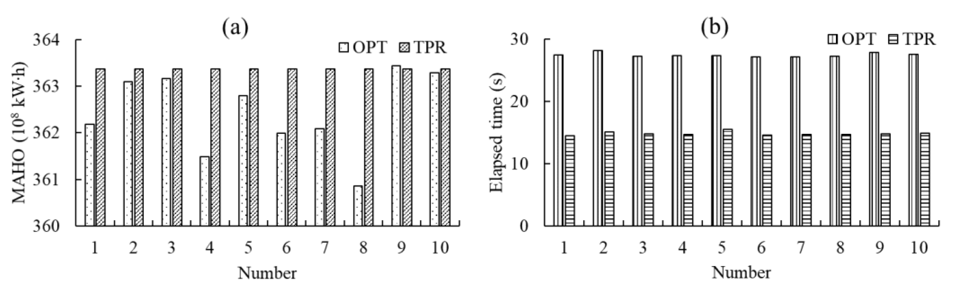
As can be seen from Figure 5a, the OPT approach-based MAHO is 0.3% (0.93 × 10⁸ kW∙h) less than the TPR rules-based MAHO on average. In only one out of ten calculations (the ninth calculation), the OPT approach-based MAHO is more than the TPR rules-based MAHO. Moreover, the standard deviations of the OPT approach-based MAHO and the TPR rules-based MAHO are 0.86 × 10⁸ kW∙h and zero, respectively, indicating that the TPR rules-based MAHO is much more stable than the OPT approach-based MAHO. From Figure 5b, it could be seen that the TPR rules-based elapsed time (14.8 s on average) is about half of the OPT approach-based elapsed time (27.4 s on average) in the MATLAB environment on the same computer, showing that the computational efficiency of TPR rules is much higher than that of the OPT approach.

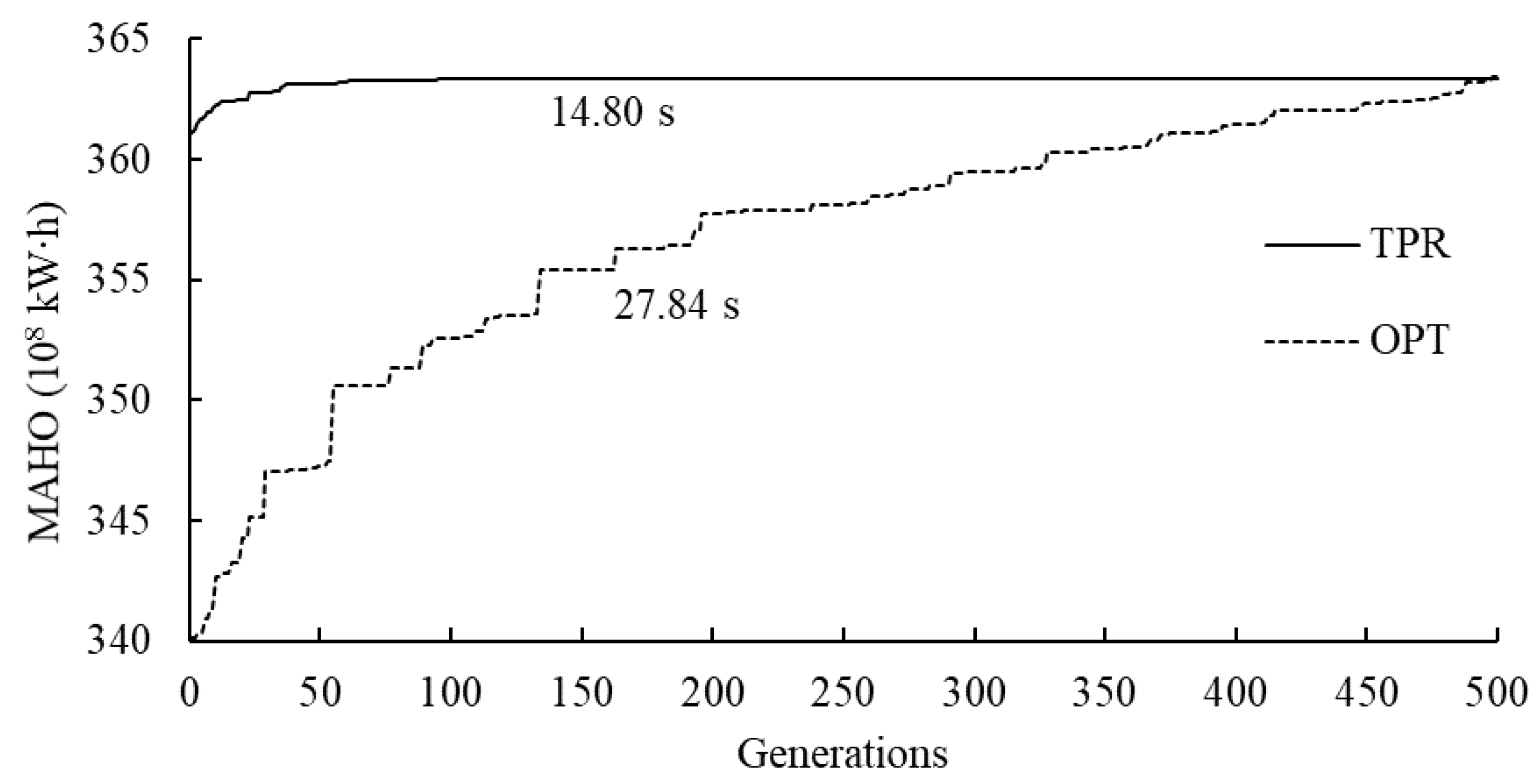
Taking the ninth calculation as an example for analysis, the optimization processes of MAHO based on the OPT approach and the TPR rules are shown in Figure 6. It could be seen that the convergence speed of the TPR rules-based MAHO is much faster than that of the OPT approach-based MAHO. Specifically, the TPR rules-based MAHO converges to a stable value (363.37 × 10⁸ kW∙h) after the 150th generation, while the OPT approach-based MAHO just reaches the same value at the 500th generation. In addition, it is noteworthy that the OPT approach-based MAHO does not reach the final stable value at the 500th generation, although the convergence speed has become very low. In other words, the OPT approach-based MAHO can exceed the TPR rules-based MAHO if the elapsed time or the maximum number of generations is not limited.

The ninth calculation results of the whole scheduling period are employed to calibrate the coefficients/parameters of the MLR, ANN, and TPR rules for the UYR multireservoir system. Moreover, the calibration details of the MLR and ANN rules could be found in Liu et al. [26]. The calibrated coefficients/parameters of the MLR and ANN rules are shown in

Table 3. MLR and ANN rules of Long and Liu reservoirs.

Reservoir	Season	LTS Rules	R
Long	Wet	S1W,I = 0.651I1W,I + 0.659S1D,i−1 + 2.14	0.340 **
		Net_Long_Wet	0.484 **
	Dry	S1D,I = 0.459I1D,I + 0.613S1W,I + 3.12	0.158 **
		Net_Long_Dry	0.454 **
Liu	Wet	S2W,i = 0.089O1W,I + 0.278I12W,I + 0.271S2W,i−1 + 1.53	0.196 **
		Net_Liu_Wet	0.376 **
	Dry	S2D,I = 0.001O1D,I + 0.309I12D,I + 0.481S2W,I + 0.22	0.310 **
		Net_Liu_Dry	0.377 **

Note: I1_W,i and I1_D,i are the inflow volumes of Long reservoir in the wet and dry seasons of the ith year, respectively; O1_W,i and O1_D,i are the outflow volumes of Long reservoir in the wet and dry seasons of the ith year, respectively; I12_W,i and I12_D,i are the interval inflow volumes between Long and Liu reservoirs in the wet and dry seasons of the ith year, respectively; S1_W,i and S1_D,i denote the WSVs of Long reservoir at the ends of the wet and dry seasons of the ith year, respectively; S2_W,i and S2_D,i denote the WSVs of Liu reservoir at the ends of wet and dry seasons of the ith year, respectively; Net_Long_Wet and Net_Long_Dry represent the ANN rules of Long reservoir during the wet season and dry season, respectively; Net_Liu_Wet and Net_Liu_Dry represent the ANN rules of Liu reservoir during the wet season and dry season, respectively; R is the Pearson correlation coefficient between the simulated WSV process and the correspondingly optimal WSV process; and ** denotes that the R value is significant under the 1% significance level.

and

Table 4. Connection weights and thresholds of two-layer FFNNs for ANN rules of Long and Liu reservoirs.

Hidden Layer Hj (j = 1−6)		H1	H2	H3	H4	H5	H6
Net_Long_Wet	W(I1, Hj)	−3.396	−1.909	−5.361	−3.958	−4.167	−6.877
	W(I2, Hj)	3.204	3.478	−1.095	−4.475	0.129	−2.492
	B(Hj)	3.148	2.601	0.446	2.197	−4.594	−1.59
	W(Hj, O)	−1.049	0.975	0.233	−0.244	−1.467	−0.296
	B(O)	−0.943
Net_Long_Dry	W(I1, Hj)	0.086	−0.589	−4.288	−0.275	0.339	3.592
	W(I2, Hj)	−1.503	6.976	−4.295	3.618	4.372	−1.79
	B(Hj)	4.231	−0.18	−0.921	−0.258	0.395	4.046
	W(Hj, O)	−0.688	−2.292	0.684	1.648	1.629	1.473
	B(O)	−0.86
Net_Liu_Wet	W(I1, Hj)	−1.167	−1.031	1.815	−0.853	−1.272	4.424
	W(I2, Hj)	0.329	1.164	0.776	−1.719	−0.796	1.605
	W(I3, Hj)	−3.161	2.898	0.294	0.389	−0.679	0.383
	B(Hj)	2.232	−0.382	−0.992	−0.372	−1.648	3.197
	W(Hj, O)	−0.907	−0.478	−1.303	−1.17	−1.611	−1.216
	B(O)	−0.507
Net_Liu_Dry	W(I1, Hj)	2.964	−1.281	−0.053	−0.359	−4.464	−0.552
	W(I2, Hj)	1.409	0.249	−0.256	2.206	1.803	1.357
	W(I3, Hj)	−0.018	−2.138	−2.941	1.084	−0.352	−2.827
	B(Hj)	−2.951	1.737	−1.017	−1.846	−2.434	3.826
	W(Hj, O)	−1.918	−0.709	0.032	0.398	0.193	1.164
	B(O)	−1.919

Note: the number of hidden neurons of two-layer FFNN is six for both Long and Liu reservoirs; W(I_i, H_j) denotes the connection weight for the ith input layer neuron and the jth hidden layer neuron; W(H_j, O) denotes the jth hidden layer neuron and the output layer neuron; B(H_j) is the threshold of the jth hidden layer neuron; and B(O) represents the threshold of the output layer neuron.

, and the parameters of the TPR rules are displayed in

Table 5. Annual, storage and release regulation parameter values of Long and Liu reservoirs.

Reservoir	Annual Regulation Parameter (φ)	Storage Regulation Parameter (λ)	Release Regulation Parameter (μ)
Long	0.490	0.050	0.943
Liu	0.982	0.000	0.122

.

As can be seen from Table 3, all regression coefficients of the MLR rules for both Long and Liu reservoirs are positive values of no more than 1. All the R values in Table 3 are significant under the 1% significance level, indicating that both the MLR and ANN rules could well describe the OPT approach-based scheduling processes. Nonetheless, all the R values are not more than 0.7, which implies that there are still some obvious differences between the OPT approach-based and the MLR/ANN rules-based scheduling processes. Moreover, combining Table 3 with Table 4, it could be seen that the MLR rules-based R values are always smaller than the ANN rules-based R values when the number of hidden neurons of two-layer FFNN is not less than 6, showing that the ANN rules have more application potential than the MLR rules.

From Table 5, it can be seen that the three regulation parameters of the TPR rules are obviously different between Long and Liu reservoirs. Specifically, the φ value of Long reservoir is less than 0.5, and the φ value of Liu reservoir is close to 1. According to the φ value, it can be deduced that the PLs of Long and Liu reservoirs are 2572.3 m and 1695.2 m, respectively. Moreover, the λ (μ) value of Long reservoir is larger than the λ (μ) value of Liu reservoir. Therefore, compared with Liu reservoir, Long reservoir not only has much stronger interannual regulation effect, but also has more obvious storage-release flexibilities.

4.2. Scheduling Effects of the TPR, MLR, and ANN Rules

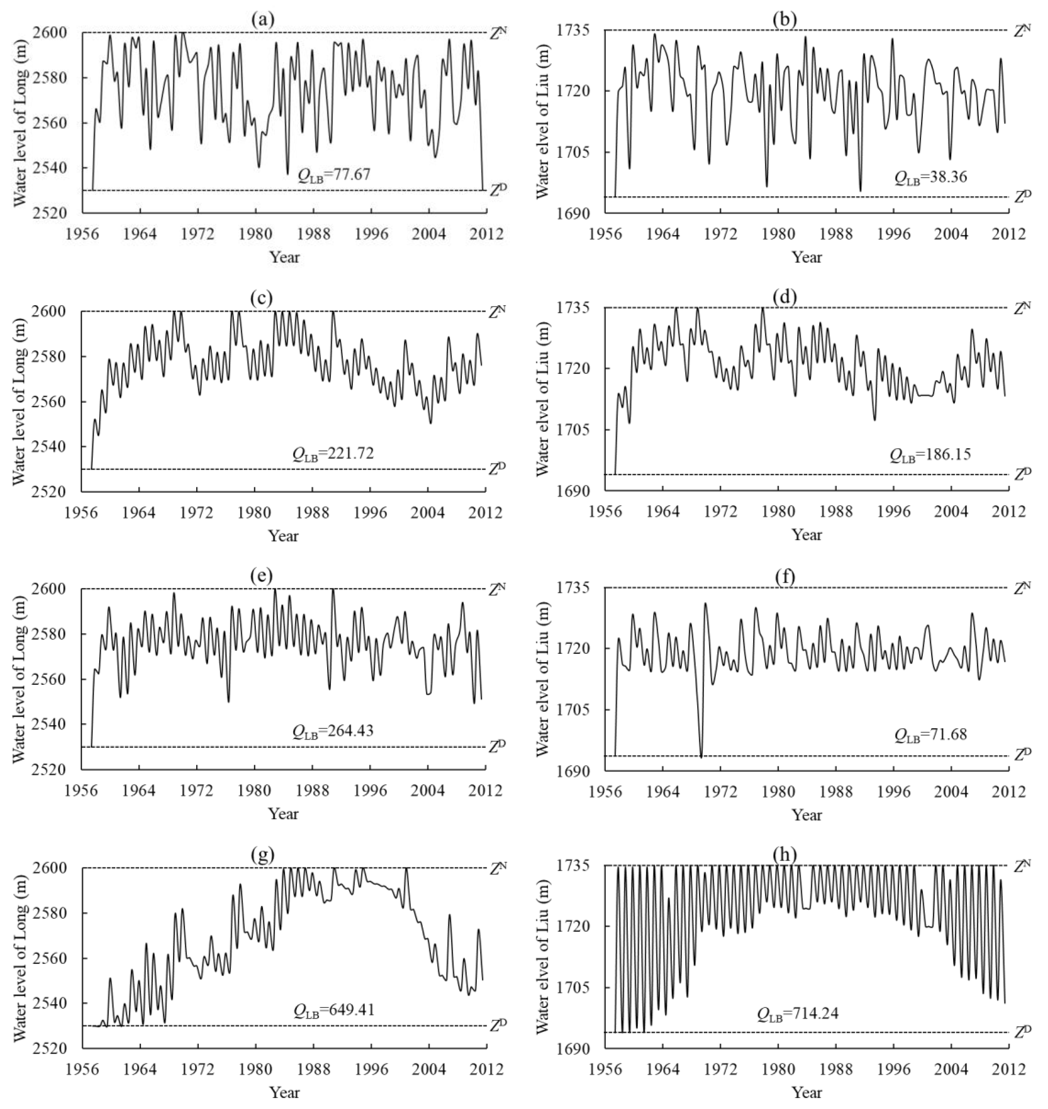
The OPT approach-based, MLR rules-based, ANN rules-based, and TPR rules-based water-level processes are shown in Figure 7. The randomness tests of water-level processes were conducted for both Long and Liu reservoirs under the significance level α = 0.01. It can be seen from Figure 7 that all the Q_LB values are much larger than χ²_1−α(10) = 23.21, indicating that all the water-level processes have strong regularity. Comparing Figure 7a,b with Figure 7c–f, the OPT approach-based Q_LB values are obviously smaller than the MLR/ANN rules-based Q_LB values for both Long and Liu reservoirs, showing that the OPT approach-based water-level processes resolved by the CS algorithm have some randomness. Comparing Figure 7a,c,e with Figure 7b,d,f, it could be found that the OPT approach-based and MLR/ANN rules-based Q_LB values of Long reservoir are also larger than those of Liu reservoir, which implies that the water-level processes of Long reservoir are more regular than those of Liu reservoir. Moreover, combining with Figure 7g,h, it can be seen that the MLR/ANN rules-based Q_LB values are significantly less than the TPR rules-based Q_LB values for both Long and Liu reservoirs, so the TPR rules-based water-level processes are more regular than the MLR/ANN rules-based water-level processes.

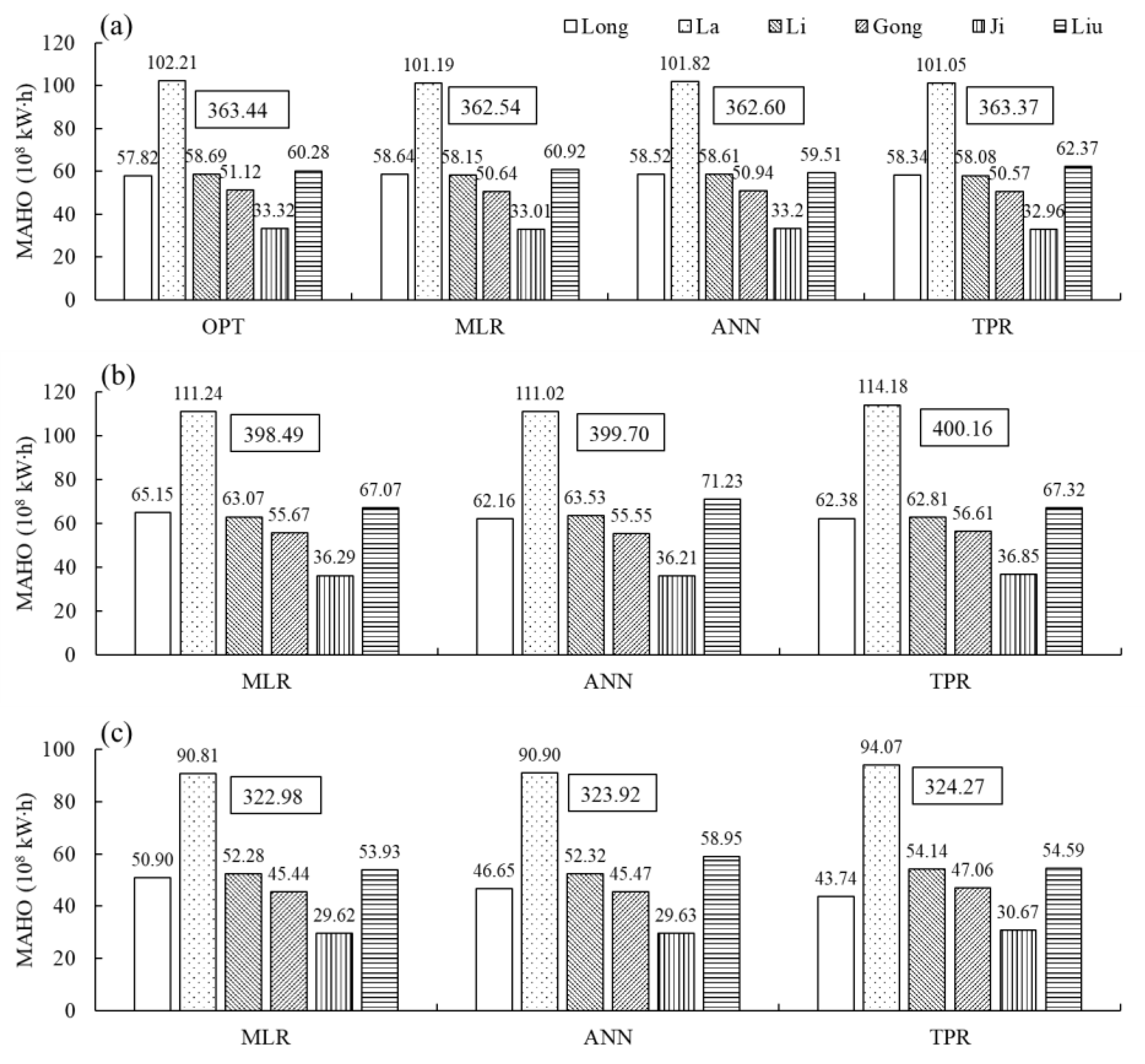
The MAHOs of six reservoirs in the UYR multireservoir system under different inflow conditions are shown in Figure 8. As can be seen from Figure 8a, for the entire system, the MLR/ANN rules-based MAHO reduces by about 0.2 % (0.86 × 10⁸ kW∙h), compared to the OPT approach-based MAHO, and is about 0.79 × 10⁸ kW∙h less than the TPR rules-based MAHO. For Long and Liu reservoirs, the variation coefficient of the MLR rules-based, ANN rules-based, and TPR rules-based MAHOs is 0.011; and for the other four hydropower reservoirs, the variation coefficient of the MLR rules-based, ANN rules-based, and TPR rules-based MAHOs is 0.004. Therefore, the TPR rules perform better than the MLR and ANN rules under the historical inflow condition. In addition, the selection of LTOS rule forms can affect the hydropower generation benefit of each reservoir at the UYR and has a greater impact on the MRS reservoirs than on the run-of-river hydropower reservoirs as a whole.

It can be seen from Figure 8b,c that significant inflow variations have important influences on the MAHO of the UYR multireservoir system. Specifically, for the entire system, the MLR rules-based, ANN rules-based, and TPR rules-based MAHOs separately increase by 9.9%, 10.2%, and 10.1% under the increased inflow condition; and the MLR rules-based, ANN rules-based, and TPR rules-based MAHOs separately reduce by 10.9%, 10.7%, and 10.8% under the reduced inflow condition. Thus, the MLR, ANN, and TPR rules are all sensitive to the reservoir inflows at the UYR. Nonetheless, for the UYR multireservoir system, the TPR rules can realize 0.1–0.4% MAHO more than the MLR and ANN rules under the increased/reduced inflow condition, showing that the TPR rules have stronger adaptability than the MLR and ANN rules.

5. Discussion

5.1. Comparison between the OPT Approach and the TPR Rules

Figure 5 and Figure 6 together show that the TPR rules are easier to achieve more MAHO for the UYR multireservoir system under the limited elapsed time or iterations. This could be explained from two aspects: the number of decision variables and the optimization model.

From the viewpoint of decision variables, the OPT approach has to determine 216 water level variables for both Long and Liu reservoirs, while the TPR rules require optimization of only six regulation parameters. With the increasing number of decision variables, the solution structure of LTOS model is more complex and the calculation process is more cumbersome, so the computational time will become longer [4,27]. In addition, the more complex the solution structure, the greater the risk of falling into a local optimum, and the more unstable and chaotic the near-optimal solution obtained in finite time [27,31,32]. As shown in Figure 7a,b,g,h, the OPT approach-based water level processes have stronger randomness than the TPR rules-based water level processes.

From the perspective of the optimization model, the LTOS model for deriving the TPR rules is a surrogate model of the LTOS model of the OPT approach. Specifically, the additional constraint Equation (10) is incorporated into the LTOS model of the OPT approach, generating the LTOS model for deriving the TPR rules, to reduce the complexity of LTOS model of the OPT approach. In the LTOS model for deriving the TPR rules, the water level, WSV, and outflow processes of an MRS reservoir are mainly controlled by three regulation parameters. Nevertheless, a surrogate model could be approximated to a complex simulation model with significantly reduced computational costs and could be used to replace the complex model for optimization [28]. Moreover, a surrogate model with a small number of controllable parameters could generate solutions that are not inferior to those of complex optimization models of reservoir scheduling [27].

5.2. Comparison between the MLR, ANN, and TPR Rules

As shown in Figure 2, the MLR and ANN rules are derived from the OPT approach-based scheduling processes. Combining Figure 7 and Figure 8, it can be seen that the MLR/ANN rules-based water level processes are more regular than the OPT approach-based water level processes for Long and Liu reservoirs, but the MLR/ANN rules-based MAHO is less than the OPT approach-based MAHO for the UYR multireservoir system. Thus, the LTOS rules derived by the indirect derivation approach could reflect the deterministic variation information of the OPT approach-based scheduling processes, and thus generate more regular scheduling processes. However, these rules make it difficult to achieve the OPT approach-based scheduling effects, because they do not reflect the uncertain variation information. From the R values in Table 3, it can also be seen that for Long and Liu reservoirs, the MLR/ANN rules-based WSVs have good relationships with the OPT approach-based WSVs, but their differences cannot be ignored. Moreover, the best-fitting effect criterion for making scheduling rules may not always be suitable for generating the best rules [23]. As shown in Figure 8, the MLR rules-based MAHOs are less than the ANN rules-based MAHOs for the UYR multireservoir system under different inflow conditions. In some other studies [24,25], it could also be found that the MLR rules perform not as well as the ANN rules due to the nonlinear characteristics of LTOS of multireservoir systems [31,32].

The MLR and ANN rules are derived by the indirect derivation approach that experiences two-time optimizations, i.e., the optimization of water level processes and the optimization of coefficients/parameters of MLR/ANN rules. By comparison, the TPR rules are derived by the direct derivation approach that needs only one-time optimization, i.e., the optimization of regulation parameters. As shown in Figure 8, the TPR rules achieve more MAHO for the UYR multireservoir system than the MLR and ANN rules under different inflow conditions. Therefore, compared to the MLR and ANN rules, the TPR rules are easier to derive and more adaptable in changing environments. Moreover, the MLR and ANN rules fail to deduce the PL for MRS reservoirs, while the TPR rules can settle the problem by means of the annual regulation parameter φ.

As can be seen from Equation (11), the TPR rules are similar to the MLR rules expressed by Equation (8). However, there are three obvious differences between the two forms of rules. Firstly, the TPR rules based on the coordination between the intra- and interannual regulation effects have a relatively solid physical basis, while the MLR rules are just a regression analysis result with statistical significance. Secondly, the TPR rules have fewer parameters than the MLR, and the regulation parameters of the TPR rules have more explicit ranges than the regression coefficients of the MLR rules. Nevertheless, the three regulation parameters of the TPR rules are between 0 and 1, which may explain why the regression coefficients of the MLR rules shown in Table 3 are not more than 1. Thirdly, the inflow variables of the TPR rules are different from those of the MLR rules. Specifically, the inflow variables of the TPR rules denote the natural inflows, while the inflow variables of the MLR rules include two parts, i.e., the release of upstream reservoirs and the local inflow.

5.3. Three Parameters of the TPR Rules

The TPR rules have three regulation parameters which can determine the three critical water levels of MRS reservoirs. Compared with the storage capacity coefficient β, the interannual regulation capacity of a reservoir can be judged more clearly by the annual regulation parameter φ. The parameter φ determines the PL of an MRS reservoir, and thus the annual and perennial storage space of the reservoir. In the LTOS of the UYR multireservoir system, Liu reservoir should not be treated as an MRS reservoir, as its β value (0.13) is obviously smaller than 0.3. However, the β value-based judgement is not so reliable because it neglects the intraannual runoff distribution and the interaction between different reservoirs in the joint operation. By comparison, these characteristics are considered in the TPR rules. As shown in Table 5, the φ value (0.982) indicates that the PL of Liu reservoir is higher than the dead water level, and thus Liu reservoir has a small size of perennial storage space for interannual regulation. The φ value (0.49) of Long reservoir shows that the perennial storage space is about half of the active storage space, and the interannual regulation capability of Long reservoir is much stronger than that of Liu reservoir. Based on the φ value, The PL of Long reservoir is 2572.3 m. By solving a multiobjective LTOS model, Wang et al. [7] suggested that in a normal year, the DL of Long reservoir should be kept at about 2570 m, which is slightly lower than 2572.3 m. That is because their study only considered the LTOS of Long reservoir, and higher water levels mean a higher risk of wasting surplus water, which is detrimental to the LTOS of Long reservoir itself.

The storage regulation parameter λ and the release regulation parameter μ jointly determine the variations of the WL and DL, respectively. Liu et al. [26] found an abrupt change in annual inflows to Long and Liu reservoirs in 1989, and a significant decline in the multiyear average volumes to both reservoirs after 1989. Combining with the values of λ and μ shown in Table 5, it can be inferred that the WL and DL of Long reservoir have an increasing trend before 1989 and a decreasing trend after 1989; and the WL of Liu reservoir has the similar variation trend with the WL of Long reservoir, but the WL of Liu reservoir varies little between years. As a result, the two MRS reservoirs could store more water until 1989 and release more water afterwards. These inferred results are confirmed in Figure 7g,h. In addition, for Long reservoir, 1971 is a dry year and 2006 is a wet year. Figure 7g shows that Long reservoir releases more water during the dry season in 1971 and stores more water during the wet season in 2006. Therefore, the parameters λ and μ can coordinate the intra- and interannual regulation effects of an MRS reservoir.

5.4. Contribution of This Study and Future Study

The PL, WL, and DL are three critical water levels of the MRS reservoir, which play significant roles in the LTOS of multireservoir systems. However, the three critical water levels have not been paid enough attention, and there is no general method that calculates them in light of developing regulating rules for MRS reservoirs in previous studies. Based on the coordination between the intra- and interannual regulation effects of MRS reservoirs, the TPR rules are developed in the study to reasonably and efficiently determine the three critical water levels for MRS reservoirs in a multireservoir system. Compared to the previous studies focused on a single MRS reservoir [11,14,15,19], this study investigates the three critical water levels of two cascade MRS reservoirs. As shown in Equations (8), (9) and (11), the connection of DL between adjacent years are also taken into account when determining the WL and DL. Moreover, the TPR rules can determine the PL, which is beyond the capabilities of other forms of LTOS rules.

In actuality, the TPR rules are a simple linear LTOS rule with three regulation parameters. As shown in Figure 8, the TPR rules-based MAHO is slightly more than the MLR/ANN rules-based MAHO for the UYR multireservoir system. As shown in Figure 6, the OPT approach-based MAHO can exceed the TPR rules-based MAHO if the elapsed time is long enough, or the maximum number of generations is large enough. Therefore, the current version of TPR rules still needs further improvement in the future. In addition, this study verifies the effectiveness of the TPR rules in a single-objective LTOS of two cascaded MRS reservoirs, but how effective is it in a multiobjective LTOS of more MRS reservoirs with more complex topology? Furthermore, how can the TPR rules be used to guide the short- and mid-term scheduling of multireservoir systems? These questions also need to be addressed in the future.

6. Conclusions

The PL, WL, and DL are three critical water levels for MRS reservoirs, and they play significant roles in the LTOS of a multireservoir system. In order to determine the three critical water levels, the TPR rules based on the coordination between the intra- and interannual regulation effects of MRS reservoirs are presented in the study. Specially, the LTOS model is established for maximizing the MAHO of a multireservoir system with one or more MRS reservoirs. The TPR rules are a linear form of LTOS rule with three regulation parameters (annual, storage, and release regulation parameters), and it is derived by using the CS algorithm to solve the LTOS model with three parameters as the decision variables. The OPT approach utilizes the CS algorithm to solve the LTOS model, with the WL and DL as the decision variables. The MLR and ANN rules are derived from the OPT approach-based water level processes. The UYR multireservoir system with two cascade MRS reservoirs (Long and Liu reservoirs) is taken as a case study, where the application effects of the TPR rules are compared to those of the OPT approach, MLR rules, and ANN rules. The main conclusions are drawn as follows.

(1) For the UYR multireservoir system, under the historical inflow condition, the TPR rules-based MAHO is 0.3% (0.93 × 10⁸ kW∙h) more than the OPT approach-based MAHO on average. Moreover, the TPR rules-based MAHO is constant, while the standard deviation of the OPT approach-based MAHO is 0.86 × 10⁸ kW∙h, and the elapsed time of the TPR rules is only half of the elapsed time of the OPT approach.

(2) For the UYR multireservoir system, under the historical inflow condition, the TPR rules-based MAHO is 0.79 × 10⁸ kW∙h more than the MLR/ANN rules-based MAHO on average. In addition, the TPR rules can realize 0.1%–0.4% MAHO more than the MLR and ANN rules when the reservoir inflow increases or reduces by 10%.

(3) According to the annual regulation parameter of the TPR rules, the PLs of Long and Liu reservoirs are 2572.3 m and 1695.2 m, respectively. Moreover, the PL of Liu reservoir is higher than the dead water level 1690 m, showing that Liu reservoir is an MRS reservoir in the joint LTOS of the UYR multireservoir system.

Therefore, TPR rules are an easy-to-obtain and adaptable LTOS rule that can reasonably and efficiently to determine the three critical water levels for MRS reservoirs in multireservoir systems.

References

- Tan, Q.F.; Wang, X.; Wang, H.; Wang, C.; Lei, X.H.; Xiong, Y.S.; Zhang, W. Derivation of optimal joint operating rules for multi-purpose multi-reservoir water-supply system. J. Hydrol. 2017, 551, 253–264. [Google Scholar] [CrossRef]
- Liu, L.; Parkinson, S.; Gidden, M.; Byers, E.; Satoh, Y.; Riahi, K.; Forman, B. Quantifying the potential for reservoirs to secure future surface water yields in the world’s largest river basins. Environ. Res. Lett. 2018, 13, 044026. [Google Scholar] [CrossRef]
- Chen, M.; Dong, Z.; Jia, W.; Ni, X.; Yao, H. Multi-objective joint optimal operation of reservoir System and analysis of objectives competition mechanism: A case study in the Upper reach of the Yangtze River. Water 2019, 11, 2542. [Google Scholar] [CrossRef] [Green Version]
- Dobson, B.; Wagener, T.; Pianosi, F. An argument-driven classification and comparison of reservoir operation optimization methods. Adv. Water Resour. 2019, 128, 74–86. [Google Scholar] [CrossRef]
- Zhang, Z.; Zhang, S.; Geng, S.; Jiang, Y.; Hui, L.; Zhang, D. Application of decision trees to the determination of the year-end level of a carryover storage reservoir based on the iterative dichotomizer 3. Int. J. Electr. Power 2015, 64, 375–383. [Google Scholar] [CrossRef]
- Ehsani, N.; Vörösmarty, C.J.; Fekete, B.M.; Stakhiv, E.Z. Reservoir operations under climate change: Storage capacity options to mitigate risk. J. Hydrol. 2017, 555, 435–446. [Google Scholar] [CrossRef]
- Wang, J.; Huang, W.; Ma, G.; Ma, G.; Wang, Y. Determining the optimal year-end water level of a multi-year regulating storage reservoir: A case study. Water Sci. Technol. Water Supply 2016, 16, 284–294. [Google Scholar] [CrossRef]
- Recio Villa, I.; Martínez Rodríguez, J.B.; Molina, J.L.; Pino Tarragó, J.C. Multiobjective optimization modeling approach for multipurpose single reservoir operation. Water 2018, 10, 427. [Google Scholar] [CrossRef] [Green Version]
- Zhang, X.Q.; Liu, P.; Xu, C.Y.; Guo, S.L.; Gong, Y.; Li, H. Derivation of hydropower rules for multireservoir systems and its application for optimal reservoir storage allocation. J. Water Resour. Plan. Manag. 2019, 145, 04019010. [Google Scholar] [CrossRef] [Green Version]
- Dittmann, R.; Froehlich, F.; Pohl, R.; Ostrowski, M. Optimum multi-objective reservoir operation with emphasis on flood control and ecology. Nat. Hazards Earth Syst. Sci. 2009, 9, 1973–1980. [Google Scholar] [CrossRef]
- Bertone, E.; O’Halloran, K.; Stewart, R.A.; de Oliveira, G.F. Medium-term storage volume prediction for optimum reservoir management: A hybrid data-driven approach. J. Clean. Prod. 2017, 154, 353–365. [Google Scholar] [CrossRef] [Green Version]
- Jiang, Z.; Song, P.; Liao, X. Optimization of year-end water level of multi-year regulating reservoir in cascade hydropower system considering the inflow frequency difference. Energies 2020, 13, 5345. [Google Scholar] [CrossRef]
- Tan, Q.F.; Wen, X.; Fang, G.H.; Wang, Y.Q.; Qin, G.H.; Li, H.M. Long-term optimal operation of cascade hydropower stations based on the utility function of the carryover potential energy. J. Hydrol. 2020, 580, 124359. [Google Scholar] [CrossRef]
- Draper, A.J.; Lund, J.R. Optimal hedging and carryover storage value. J. Water Resour. Plan. Manag. 2004, 130, 83–87. [Google Scholar] [CrossRef] [Green Version]
- Zhao, T.; Zhao, J.; Liu, P.; Lei, X. Evaluating the marginal utility principle for long-term hydropower scheduling. Energy Convers. Manag. 2015, 106, 213–223. [Google Scholar] [CrossRef] [Green Version]
- You, J.Y.; Cai, X. Hedging rule for reservoir operations: 1. A theoretical analysis. Water Resour. Res. 2008, 44, W01415. [Google Scholar] [CrossRef]
- Chang, J.X.; Guo, A.J.; Wang, Y.M.; Ha, Y.P.; Zhang, R.; Xue, L.; Tu, Z.Q. Reservoir operations to mitigate drought effects with a hedging policy triggered by the drought prevention limiting water level. Water Resour. Res. 2019, 55, 904–922. [Google Scholar] [CrossRef]
- Liu, J.; Huang, C.H.; Zeng, G.Z. Comparative analysis of year-end water level determining methods for cascade carryover storage reservoirs. IOP Conf. Ser. Earth Environ. Sci. 2017, 82, 12060. [Google Scholar] [CrossRef] [Green Version]
- Chou, F.N.F.; Wu, C.W. Stage-wise optimizing operating rules for flood control in a multi-purpose reservoir. J. Hydrol. 2015, 521, 245–260. [Google Scholar] [CrossRef]
- Peng, Y.; Zhang, X.; Zhou, H.; Wang, B. A method for implementing the real-time dynamic control of flood-limited water level. Environ. Earth Sci. 2017, 76, 742. [Google Scholar] [CrossRef]
- Liu, G.; Qin, H.; Shen, Q.; Tian, R.; Liu, Y. Multi-objective optimal scheduling model of dynamic control of flood limit water level for cascade reservoirs. Water 2019, 11, 1836. [Google Scholar] [CrossRef] [Green Version]
- Aboutalebi, M.; Haddad, O.B.; Loáiciga, H.A. Optimal monthly reservoir operation rules for hydropower generation derived with SVR-NSGAII. J. Water Resour. Plan. Manag. 2015, 141, 04015029. [Google Scholar] [CrossRef] [Green Version]
- Liu, P.; Li, L.; Chen, G.; Rheinheimer, D.E. Parameter uncertainty analysis of reservoir operating rules based on implicit stochastic optimization. J. Hydrol. 2014, 514, 102–113. [Google Scholar] [CrossRef]
- Zhang, D.; Lin, J.; Peng, Q.; Wang, D.; Yang, T.; Sorooshian, S.; Liu, X.; Zhuang, J. Modeling and simulating of reservoir operation using the artificial neural network, support vector regression, deep learning algorithm. J. Hydrol. 2018, 565, 720–736. [Google Scholar] [CrossRef] [Green Version]
- Niu, W.J.; Feng, Z.K.; Feng, B.F.; Min, Y.W.; Cheng, C.T.; Zhou, J.Z. Comparison of multiple linear regression, artificial neural network, extreme learning machine, and support vector machine in deriving operation rule of hydropower reservoir. Water 2019, 11, 88. [Google Scholar] [CrossRef] [Green Version]
- Liu, S.; Xie, Y.; Fang, H.; Huang, Q.; Huang, S.; Wang, J.; Li, Z. Impacts of inflow variations on the long term operation of a multi-hydropower-reservoir system and a strategy for determining the adaptable operation rule. Water Resour. Mang. 2020, 34, 1649–1671. [Google Scholar] [CrossRef]
- Koutsoyiannis, D.; Economou, A. Evaluation of the parameterization-simulation-optimization approach for the control of reservoir systems. Water Resour. Res. 2003, 39, 1170. [Google Scholar] [CrossRef] [Green Version]
- Tsoukalas, I.; Makropoulos, C. Multiobjective optimisation on a budget: Exploring surrogate modelling for robust multi-reservoir rules generation under hydrological uncertainty. Environ. Model. Softw. 2015, 69, 396–413. [Google Scholar] [CrossRef]
- Zhang, X.; Yu, X.; Qin, H. Optimal operation of multi-reservoir hydropower systems using enhanced comprehensive learning particle swarm optimization. J. Hydrol. Environ. Res. 2016, 10, 50–63. [Google Scholar] [CrossRef]
- Feng, M.; Liu, P.; Guo, S.; Gui, Z.; Zhang, X.; Zhang, W.; Xiong, L. Identifying changing patterns of reservoir operating rules under various inflow alteration scenarios. Adv. Water Resour. 2017, 104, 23–36. [Google Scholar] [CrossRef]
- Reddy, M.J.; Kumar, D.N. Optimal reservoir operation using multi-objective evolutionary algorithm. Water Resour. Manag. 2006, 20, 861–878. [Google Scholar] [CrossRef] [Green Version]
- Allawi, M.F.; Jaafar, O.; Mohamad, H.F.; Abdullah, S.M.S.; El-shafie, A. Review on applications of artificial intelligence methods for dam and reservoir-hydro-environment models. Environ. Sci. Pollut. Res. 2018, 25, 13446–13469. [Google Scholar] [CrossRef] [PubMed]
- Ming, B.; Chang, J.X.; Huang, Q.; Wang, Y.M.; Huang, S.Z. Optimal operation of multi-reservoir system based on cuckoo search algorithm. Water. Resour. Manag. 2015, 29, 5671–5687. [Google Scholar] [CrossRef]
- Meng, X.; Chang, J.; Wang, X.; Wang, Y. Multi-objective hydropower station operation using an improved cuckoo search algorithm. Energy 2019, 168, 425–429. [Google Scholar] [CrossRef]
- Fisher, T.J.; Gallagher, C.M. New weighted portmanteau statistics for time series goodness of fit testing. J. Am. Stat. Assoc. 2012, 107, 777–787. [Google Scholar] [CrossRef]
- Xie, Y.; Huang, S.; Liu, S.; Leng, G.; Peng, J.; Huang, Q.; Li, P. GRACE-based terrestrial water storage in Northwest China: Changes and Causes. Remote Sens. 2018, 10, 1163. [Google Scholar] [CrossRef] [Green Version]
- Nematollahi, B.; Niazkar, M.; Talebbeydokhti, N. Analytical and numerical solutions to level pool routing equations for simplified shapes of inflow hydrographs. Iran J. Sci. Technol. Trans. Civ. Eng. 2021, in press. [Google Scholar] [CrossRef]
- Li, X.Z.; Chen, Z.J.; Fan, X.C.; Cheng, Z.J. Hydropower development situation and prospects in China. Renew. Sustain. Energy Rev. 2018, 82, 232–239. [Google Scholar] [CrossRef]
- Xu, B.; Zhang, C.; Jiang, Y.; Huang, Q.; Wang, G.; Guan, T. Reliability-resilience-vulnerability of water supply system and its response relationship to multiple factors. J. Hydraul Eng. 2020, 51, 1502–1513. [Google Scholar] [CrossRef]
Figure 1.
Diagrammatic sketch of the PL, WL, and DL of an MRS reservoir. (Note: ZN, ZF, and ZD are the normal water level, the flood limit water level, and the dead water level, respectively; ZP denotes the PL; ZW,i and ZD,i represent the WL and the DL of the ith year, respectively; VW,i and VD,i denote the increased WSV in the wet season and the reduced WSV in the dry season at the ith year, respectively; VA and VP represent the annual and the perennial storage spaces, respectively; and SD and SA denote the dead and the active storage spaces, respectively).
Figure 2.
Flow chart of deriving the MLR, ANN, and TPR rules.
Figure 3.
Relative locations of hydrological stations and hydropower reservoirs at the UYR.
Figure 4.
Annual runoff processes of TNH (a), GD (b), XH (c), and XC (d) stations at the UYR (Note: the number in the box denotes the multiyear average runoff volume.).
Figure 5.
MAHO (a) and elapsed time (b) results based on the OPT approach and the TPR rules (Note: all calculations were realized in the MATLAB environment on the same computer).
Figure 6.
Optimization processes of MAHO of UYR multireservoir system based on the OPT approach and the TPR rules in the ninth calculation.
Figure 7.
The OPT approach-based (a,b), MLR rules-based (c,d), ANN rules-based (e,f), and TPR rules-based (g,h) water-level processes (Note: (a,c,e,g) show the water level processes of Long reservoir, and (b,d,f,h) display the water-level processes of Liu reservoir).
Figure 8.
MAHOs of six hydropower reservoirs in the UYR multireservoir system under different inflow conditions (Note: (a) denotes the historical inflow condition; (b,c) represents the increased/reduced inflow condition; and the number in the box denotes the MAHO of the UYR multireservoir system).