Computational Fluid Dynamics Modeling of Hollow Membrane Filtration for Concentration Polarization

Abstract

Based on CFD and film theory, filtration’s two-dimensional CFD model of the hollow membrane was established by integrating the mass transformation and the hydrodynamic transportation. Parameters of concentration polarization in the membrane channel (i.e., solute mass concentration, concentration polarization factors, and concentration polarization layer thickness) were estimated under different hydraulic conditions. In addition, the algorithm for the thickness of the concentration polarization layer has been improved. The results showed that decreasing the feed Reynolds number or increasing the transmembrane pressure can enhance the concentration polarization phenomena. Concentration polarization parameters increased sharply at the initial place (X/H < 25, where H is the entrance width, X is the distance from entrance) and then flatten out (X/H > 25) along the membrane channel; solute concentration and concentration polarization factors were arranged in a U-shape in the membrane channel’s cross-section. The improved algorithm could match well with cross section data, $\frac{{\delta }_2}{H}$ at X/H = 1, 25, and 200 are 0.038, 0.11, and 0.25, respectively, which can reasonably reflect the distribution of the concentration polarization phenomenon in the membrane channel.

1. Introduction

During the past decades, membrane technologies have played an increasingly important role in the industrial separation process and water treatment field. Many studies have focused on the best ways of using a particular membrane process [1,2]. Computational fluid dynamics (CFD) techniques can provide an effective approach to examine membrane technologies. With the development of the increasingly delicate CFD commercial software [3], membrane filtration processes can be easily modeled directly and visualized to realize the membrane process optimization and improvement, which make the CFD technology a viable and prevailing tool for analysis of membrane filtration systems [4,5,6].

Previous studies about CFD technology paid attention to the hydrodynamics and the fluid flow pattern adjacent to the membrane, which can distinctly impact the permeation and solute rejection mechanism across the membrane [7,8,9,10]. But these studies may provide incorrect predictions for the phenomenon based on film theory and assuming the membrane as an impermeable wall with zero concentration build-up and zero mass transmembrane transportation [11,12,13]. To further study the problem, Wiley and Fletcher [14] established a two-dimensional (2D) CFD simulation with the commercial finite control volume simulator CFX 4, integrating the wall concentration with the adjacent fluid hydrodynamics to predict concentration polarization [15]. Ahmad and Lau [12,16] integrated CFD simulation of concentration polarization in a narrow membrane channel, with the CFD software Fluent v6. The User-Defined Function (UDF) has been adopted to describe the concentration polarization under the laminar flow pattern based on the film theory and mass transmembrane transportation adopting the rejection coefficient R. Using the same method, Ahmad [17] investigated the hydraulic condition and concentration polarization under the turbulent flow in the spacer-filled channel. Amokrane [4] studied the concentration polarization in the spacer-filled spiral wound membrane by simplifying the film theory and taking into the rejection coefficient R > 0.99.

These studies have solved the CFD limitations that concentration build-up and mass transmembrane transportation were ignored, and they conducted the filtration modeling for the plate membrane or spiral wound membrane. However, few studies have focused on the tubular membrane or hollow membrane. Recently, researchers usually combined the Darcy formula and convection–diffusion equation to predict the concentration polarization in the 2D CFD model despite the good compatibility of the traditional film theory with CFD software [18,19,20]. This study focused on the CFD simulation of the concentration polarization of the hollow membrane. which few studies had focused on. The hollow membrane filtration’s 2D CFD model was established based on the film theory in this study. Concentration build-up and transmembrane transportation had been taken into consideration with CFD software Ansys Fluent 15.0. Concentration polarization parameters in the membrane channel (i.e., solute mass concentration, concentration polarization factors, and concentration polarization layer thickness) were investigated under different hydraulic conditions. In this study, the calculation method of the thickness of the concentration polarization layer is optimized to overcome the shortcomings of small values and to better couple the cross-sectional analysis data.

2. Materials and Methods

2.1. Geometry and Computational Mesh

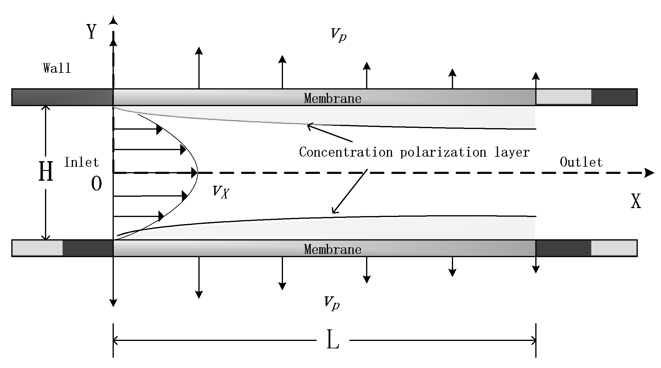
The hollow fiber membrane module usually contained a lot of fibers. Every fiber was assumed identical and only one fiber was modeled, as shown in Figure 1. The x–y Cartesian coordinate system was established as coordinate origin ‘O’ was defined. Figure 1 showed the original liquid inlet on the left and the concentrate outlet on the right, with the permeate flowing out from above and below the model at a flow rate of V_p, and V_x represents the parabolic flow velocity, and this model is equivariantly symmetric. The simulated domain was 200 mm in length and 1 mm in height. The distance of the membrane adjacent node to the membrane was 1 × 10⁻⁶ m. The rectangular grid was applied. The number of grid points along the length direction was increased to 2000 to reduce the aspect ratio. The computational grid was constructed with 2000 × 50 cells. In order to precisely predict the mass concentration, about 85% of grids were allocated at the near membrane region due to the high concentration profile adjacent to the membrane interface. The meshes within an optimal quality of one accounted for more than 90% of all the meshes in the entire model. Moreover, the mesh quality was favorable and exhibited a stable distribution.

2.2. Governing Equations

In 2D-cylindrical coordinates, the governing equations including the mass conservation equation, the momentum conservation equation, and the mass concentration conservation equation are mathematically given in Equations (1)–(4).

Continuity equation:

$$\rho \left(\frac{\partial v_X}{\partial x}+\frac{\partial v_y}{\partial y}\right)=0$$

(1)

Momentum conservation equation (Navier-Stokes equations):

$$X: \rho v_X\frac{\partial v_X}{\partial x}+\rho v_Y\frac{\partial v_X}{\partial y}=-\frac{\partial P}{\partial x}+\mu \left(\frac{{\partial }^2{v}_X}{\partial x^2}+\frac{{\partial }^2{v}_X}{\partial y^2}\right)$$

(2)

$$Y: \rho v_X\frac{\partial v_Y}{\partial x}+\rho v_Y\frac{\partial v_Y}{\partial y}=-\frac{\partial P}{\partial x}+\mu \left(\frac{{\partial }^2{v}_Y}{\partial x^2}+\frac{{\partial }^2{v}_Y}{\partial y^2}\right)$$

(3)

Convection–diffusion equation (Mass transfer or solute transport equation):

$$\frac{\partial C}{\partial t}+v_X\frac{\partial C}{\partial x}+v_Y\frac{\partial C}{\partial y}=D\left(\frac{{\partial }^{2}C}{\partial x^2}+\frac{{\partial }^{2}C}{\partial y^2}\right)$$

(4)

where $x$ and $y$ are displacements in $X$ and $Y$ directions; $\rho$ is the density of the solution; $v_X$ and $v_Y$ are flow velocity of the solution in $X$ and $Y$ directions; C is the concentration of the solution; D is the molecular diffusion coefficient of the solute in water.

The hydraulic condition profile can be obtained by the dispersing continuity equation and the momentum conservation equation; the mass concentration distribution profile can be obtained by the dispersing convection–diffusion equation [12,21]. For the feed material condition, a solute (A)-solvent (B) system (NaCl and water) was defined. Because the Reynolds number (Re) is smaller than 1300, the flow is the incompressible laminar.

2.3. Simulation Conditions

The filtration solution was used with a mass concentration of 2 g/kg NaCl solution, and the physical properties of the NaCl solution were referred to V.t. Geraldes’ study [21], and the values have been summarized in

Table 1. Solution physical properties for NaCl, valid for ( $m_A<90\mathrm{g}/\mathrm{kg}$).

Viscosity $\mathit{\mu }\left({10}^{-3} \mathbf{P}\mathbf{a}·\mathbf{s}\right)$	Binary Diffusion Coefficient ${\mathit{D}}_{\mathit{A}\mathit{B}}\left({10}^{-9}\frac{{\mathbf{m}}^2}{\mathbf{s}}\right)$	Density $\mathit{\rho }\left(\frac{\mathbf{k}\mathbf{g}}{{\mathbf{m}}^3}\right)$
$0.89\left(1+1.63m_A\right)$	$m_A<0.0061.61\left(1-14m_A\right)$	$997.1+694m_A$

. $\rho$ is the density of the NaCl solution. $m_A$ is the mass concentration of the NaCl solution. According to de Pinho’s study [11], Permeation flux ($J_V$), mass concentration in penetrants ($m_{Ap}$), and rejection coefficient (R) under transmembrane pressure (TMP) of 2 MPa, 3 MPa, and 4 MPa are all shown in

Table 2. Simulation parameters.

TMP $\Delta \mathrm{P}\left(\mathrm{MPa}\right)$	${\mathit{J}}_{\mathit{V}}$ $\left({10}^{-5}\frac{\mathbf{m}}{\mathbf{s}}\right)$	${\mathit{m}}_{\mathit{A}\mathit{p}}$ $\left(\frac{\mathrm{mg}}{\mathrm{kg}}\right)$	R	Re
2	1.24	592	0.704	250
3	1.84	442	0.779	250
4	2.37	349	0.825	250/500/1250

. The laminar flow regime (Re < 1300), Re (250/500/1250) is also shown in Table 2.

2.4. Initial and Boundary Conditions

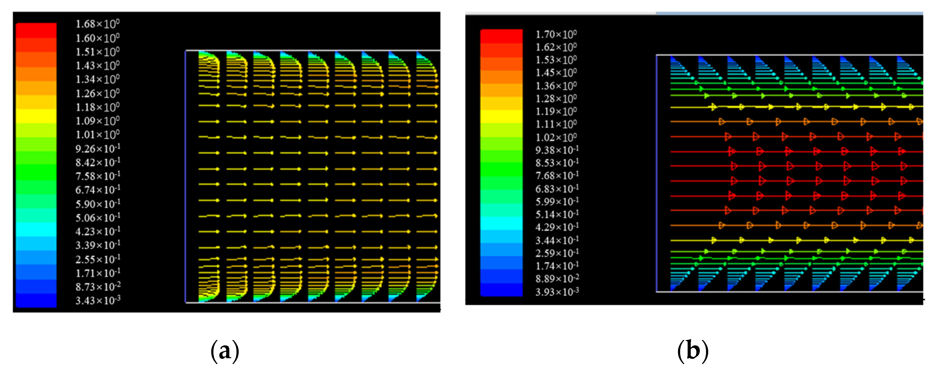
For $x=0$, $\frac{H}{2}<y<\frac{H}{2}$ plug flow was usually defined in previous studies, especially for plate membrane’s or spiral wound membrane’s inlet [4,12]. However, they did not conform to the actual hydraulic condition at the inlet of the hollow membrane. For the hollow membrane, the parabolic flow was used. The flow is assumed to be fully developed and a parabolic flow is applied. The parabolic flow field was described by Equation (5). When the Reynolds number is 1250, the inlet state distributions of the plug flow and parabolic flow were shown in Figure 2. Since the fluid has already developed before entering the hollow membrane, the use of a parabola flow was more in line with the actual situation.

$$v_X{=v}_{X,max}\times \left(1-{\left(\frac{y}{H}\right)}^2\right)v_Y{=0;m=m}_{A0}$$

(5)

For $0<x<\mathrm{L},$ $y=\text{±}\frac{H}{2}$,$m_A{=m}_{Aw}$ the no-slip condition is when $v_X=0$ was fixed for the wall. If $J_V$ was consistent with the direction of the permeated velocity ($v_Y$), $J_V$ took the positive sign, otherwise it took the negative sign. Due to the limitation of the solver, which is limited to the prediction of hydrodynamic conditions for fluids near the membrane, it is assumed that the membrane is an impermeable wall with zero concentration accumulation. This assumption ignores the mass transfer across the membrane and may lead to an incorrect assessment of the concentration polarization phenomenon. The membrane wall surface will be defined as wall, and the concentration polarization will be coupled to the custom function file UDF.

For $0<x<\mathrm{L},-\frac{H}{2}<y<\frac{H}{2}$ and since the membrane was defined as a wall, UDF was introduced to describe the concentration polarization near the membrane adjacent cells [12]. The mass concentration profile on or near the membrane can be defined by Equation (8), which specified the relationship between the mass concentration in the membrane channel ${(m}_{Ac})$, where ${\delta }_c$ was away from the membrane surface and mass concentration on the membrane surface $\left(m_{Aw}\right)$. $J_V$ and mass concentration in permeate $\left(m_{Ap}\right)$ were constants as shown in Table 2.

$$v_X=0 v_Y=\pm J_{V } D\left(\frac{\partial m_A}{\partial y}\right)+J_V{m}_A=J_V{m}_{Ap}$$

(6)

$$Y=\pm \frac{H}{2} m_A=m_{Aw} y={\delta }_c m_A=m_{Ac}$$

(7)

where $J_v$ is the water flux.

Integrating (6) with (7),

$$m_{Aw}=exp\left(\frac{J_v{\delta }_c}{D}\right)\frac{1}{R+\left(1-R\right)exp\left(\frac{J_v{\delta }_c}{D}\right)} m_{Ac}$$

(8)

For $x=\mathrm{L},-\frac{H}{2}<y<\frac{H}{2}$ the flow is fully developed at the outlet.

$$\frac{\partial v_X}{\partial x}=0 \frac{\partial v_Y}{\partial y}=0 \frac{\partial C}{\partial x}=0$$

(9)

2.5. UDF

UDF is written in C language. It is a user interface provided by Ansys Fluent 15.0, through which users can interact with the soft data to deal with some problems, as the definition of special boundary conditions or material properties was not possible to be solved with the standard module. Using CFD software fluent v6 user-defined function can define the parabolic flow in the membrane ($v_X$, Equation (5)) and mass concentration on the membrane surface ($m_{Aw}$, $m_{Ac}$, Equation (8)). Equation (8) that described the concentration distribution of the substance on the membrane wall and its vicinity cannot be solved in Fluent. This problem can be solved smoothly by writing code through UDF. Boundary conditions were redefined after each UDF iteration.

2.6. Numerical Solution

An Intel^® Core™ i7-4790K CPU 4.0 GHz with 32 GB of RAM was used for the numerical tests. Ansys Fluent (version 15.0), a finite volume method (FVM) CFD tool was used to solve the governing equations. The method in this study was similar to the A.L. Ahmad study [12]. Pressure, together with velocity, was solved using the SIMPLE algorithm, which will be used as a pressure correction equation to obtain the necessary corrections to the pressure and velocity fields and the surface mass fluxes to satisfy continuity. In discretization of the equations, least-squares cell-based second order upwind was used to deal with a gradient; second order algorithm was applied to pressure; second order upwind was chosen for momentum and the concentration of NaCl. Convergence criteria were fixed to 0.001%. As mass transfer reaches a steady state in a very short period, it is not necessary to solve the transient mass transfer equation for a given velocity field in order to obtain concentration profiles within the feed stream [22]. Thus, steady or stationary models were applied in this study.

2.7. Development of Predicted Models

Two methods were used to evaluate the thickness of the concentration polarization layer ($\delta$). In the process of membrane separation, water and small molecules permeate the membrane. The macromolecular solutes are trapped by the membrane and accumulate on the membrane surface, making the concentration $(m_{Aw})$ of the solute at the membrane surface higher than the concentration ${(m}_{A0})$ of the solute in the main solution; thus, the concentration difference ($m_{Aw}-m_{A0})$ is formed in the boundary layer near the film. Equation (10) represents the method deduced according to the film theory in the previous study [12]; Equation (11) represents the improved method, which assumed that δ is approximately equal to the distance from the membrane surface where the value of concentration $(m_A)$ is close enough to the inlet value of concentration ${(m}_{A0})$.

Method 1:

$$\delta =ln\left(\frac{m_{Aw}-m_{AP}}{m_{A0}-m_{AP}}\right)\times \frac{D_{AB}}{J_V}$$

(10)

Method 2:

$$\frac{m_A-m_{A0}}{m_{A0}}<0.001$$

(11)

Wall shear stress, ${\tau }_w$, will be evaluated from the simulation data which can be represented by:

$${\tau }_w=\mu \frac{d{v}_X}{dy}$$

(12)

Concentration polarization factor, Γ, will be evaluated according to this relation:

$$\Gamma =\frac{m_{Aw}}{m_{A0}}-1$$

(13)

For a better understanding of the influence of locations on simulation results, dimensionless channel length (X/H), height (Y/H), and concentration polarization layer thickness $\left(\frac{\delta }{H}\right)$ were applied in this study.

3. Results

3.1. The TMP Effect on Concentration Polarization

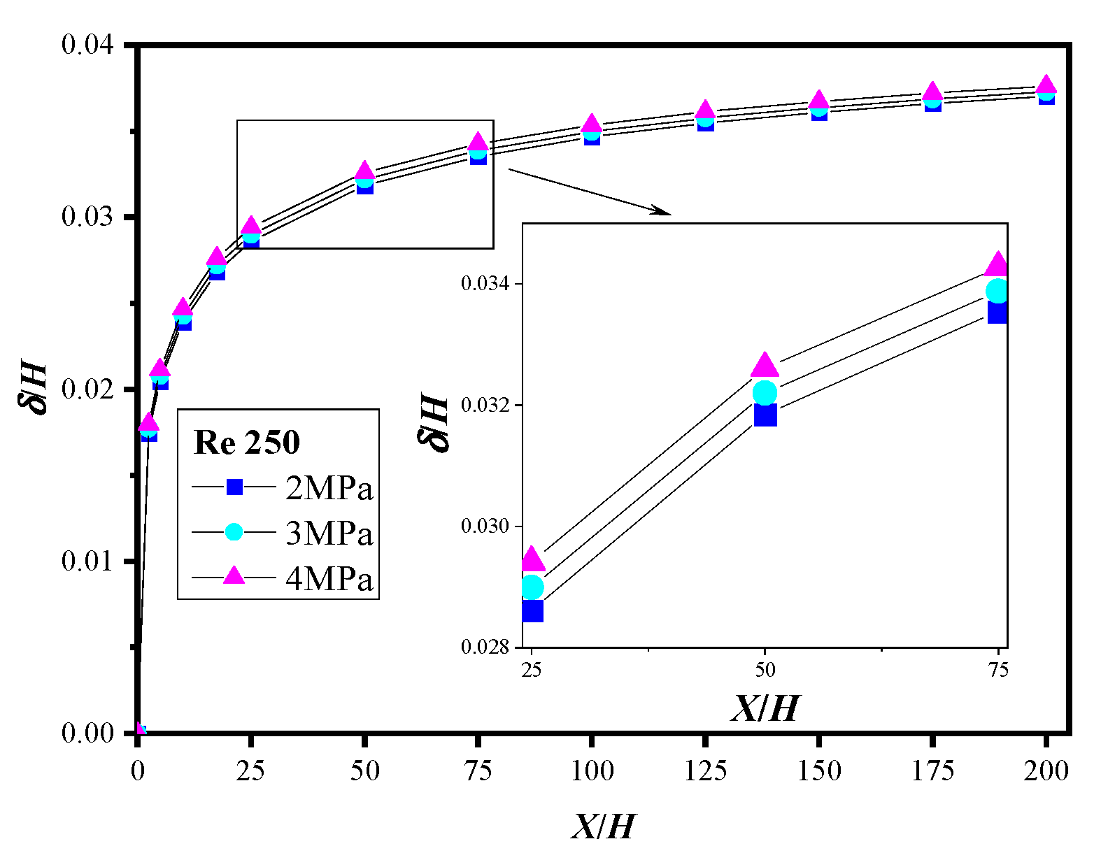
The effect of TMP on concentration polarization is shown in Figure 3. With the increase of X/H, the growth trend of $\delta$/H for 2 MPa, 3 MPa, and 4 MPa is approximately the same, all growing rapidly at X/H (0–25) and tending to level off at X/H (>25). The increment in TMP promoted the formation of the concentration polarization layer, which was consistent with the previous study [11]. The $J_V$ nearly doubled when TMP increased from 2 MPa to 4 MPa (Table 2), which led to a more solute rejection or adsorption by the membrane. This accounted for the larger $\delta$ and the stronger concentration polarization. When TMP increased from 2 MPa to 4 MPa, the thickness of the concentration polarization increased slightly, as shown in Figure 3. The TMP of 4 MPa was adopted in the subsequent section for the more obvious concentration polarization.

3.2. The Distribution of m_A and Γ in the Membrane Channel

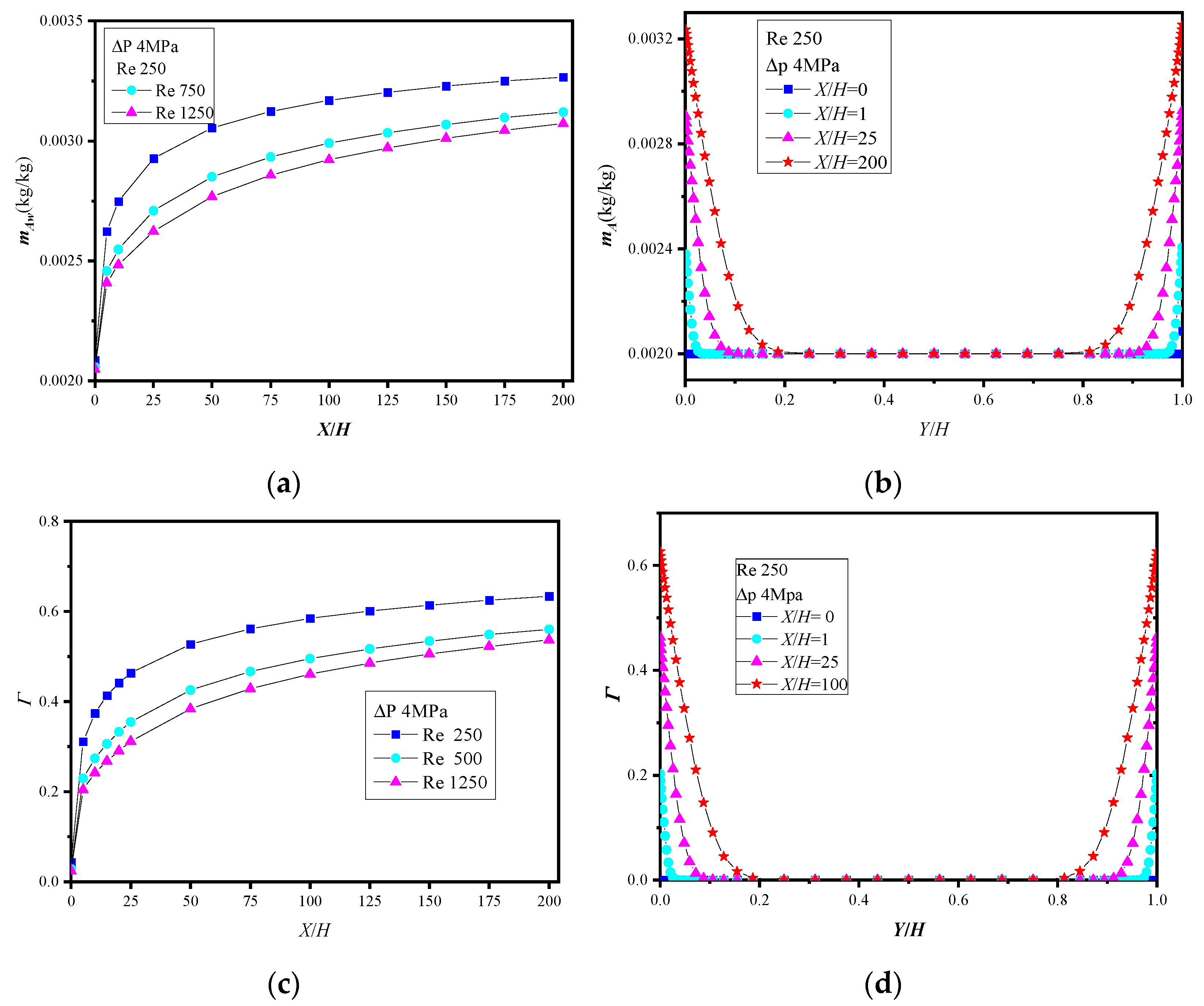
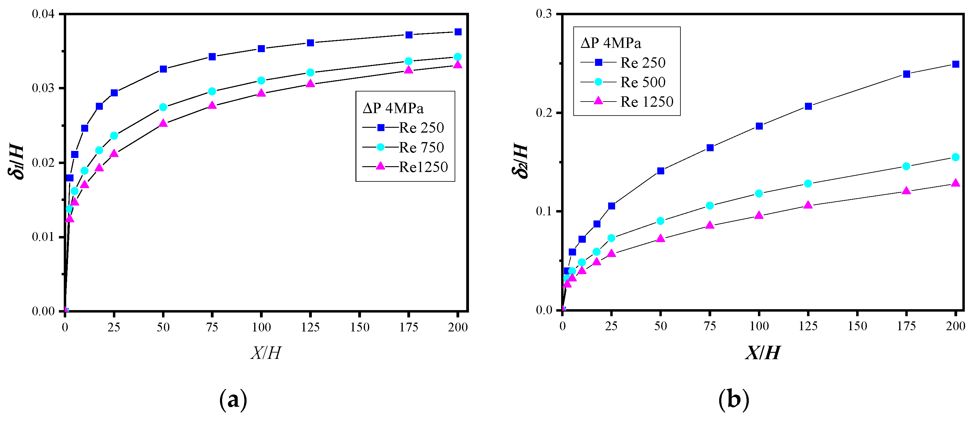
The distribution of NaCl mass concentration $(m_A)$ and concentration polarization factor (Γ) were presented in Figure 4. The distribution curves were similar because the $\Gamma$ is proportional to $m_A$, according to Equation (13). During cross-flow UF, solutes within the feed stream were forced to convect to the membrane surface due to the permeate drag, and they were accumulated near the membrane surface. Solutes within the higher concentration layer near the membrane surface tend to diffuse away from the membrane surface due to the concentration gradient. The mass transport was described by the convection–diffusion Equation (4). The steady-state of concentration polarization was established when reaching an equilibrium for convection and diffusion [22]. As shown in Figure 4c, concentration polarization increased sharply (X/H < 25), and then leveled off, which was correlated with the flow pattern in the membrane channel. Figure 5 illustrates the flow development: the maximum velocity at the inlet (X/H < 25) decreased, which led to rapid accumulation of solutes near the membrane (Figure 4a), and then the maximum velocity reached a constant, which accounted for the slow accumulation of solutes near the membrane (Figure 4a). $m_A$ at the cross-section of X/H = 0 (inlet), 1, 125, and 200 (outlet) is shown in Figure 4b. $m_A$ was 2 g/kg (Γ = 0, Figure 4d), and this result inferred that concentration polarization did not happen at the inlet. This is consistent with Equation (5), which assumed that the concentration at the entrance is constant. $m_A$ (Figure 4b) and $\Gamma$ (Figure 4d) were arranged in a U-shape in the membrane channel’s cross-section. The farther the distance from the entrance, the more the area of $m_A$ was greater than 2 g/kg or $\Gamma$ was greater than 1, which meant the greater the area of concentration polarization occurred. It was easy to deduce that the $\Delta \left(\frac{Y}{H}\right)$ was just the concentration polarization layer thickness ($\delta$). The $\Delta \left(\frac{Y}{H}\right)$ increased from 0.04 at X/H = 1 to 0.25 at X/H = 200 (Figure 4b). The concentration polarization increased along the membrane channel (X-axis direction), and $\Gamma$ increased from 0.21 at X/H = 1 to 0.63 at X/H = 200 (Figure 4d).

3.3. The Influence of Re on Concentration Polarization

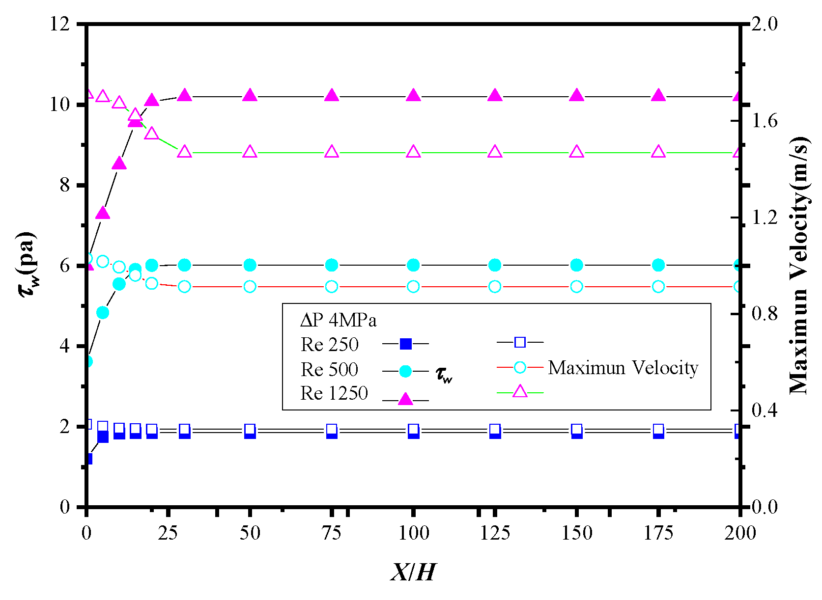
${\tau }_w$, increasing when Re increases, can decrease concentration polarization by increasing the turbulence and promoting the mass transportation near the membrane surface. Thus, $m_{Aw}$, $\Gamma$, and $\delta$ in Figure 4a,c and Figure 6b, respectively, all decreased as Re increased. ${\tau }_w$ increased rapidly near the membrane inlet region and then exhibited a nearly constant trend (Figure 5). It was decided by the relative velocity, $\frac{d{v}_X}{dy}$, which could be explained by Equation (12) that ${\tau }_w$ was proportional to $\frac{d{v}_X}{dy}$. After the fluid is contacted with the membrane surface, relative speed increased rapidly, which led to ${\tau }_w$ increasing. Then, ${\tau }_w$ reached a constant as it approached the fully developed region. This also could explain the slow increase of concentration polarization parameters ($m_{Aw}$, Γ and δ) in the fully developed region.

$\frac{{\delta }_1}{H}$ along the X-direction according to method 1 is displayed in Figure 6a. $\frac{{\delta }_1}{H}$ was 0.0075, 0.029, and 0.037, respectively, at places of X/H = 1, 25, and 200. But according to the previous analysis, $\Delta \left(\frac{Y}{H}\right)$ was also $\frac{{\delta }_1}{H}$. At each corresponding place in Figure 4b, $\frac{{\delta }_1}{H}$ was 0.04, 0.10, and 0.25, respectively. The deviation was obvious. $\frac{{\delta }_2}{H}$ along the X-direction according to method 2 was displayed in Figure 6b. At each corresponding place in Figure 6b, $\frac{{\delta }_2}{H}$ was 0.038, 0.11, and 0.25, respectively, which was in accordance with $\Delta \left(\frac{Y}{H}\right)$. Method 1 was applied in literature [12]; $\Delta \left(\frac{Y}{H}\right)$ is 1.76 (0.3/0.17) times larger than $\frac{{\delta }_1}{H}$. Obviously, this may lead to wrong conclusions. The deviation came from the wall boundary condition, which ignored the hydrodynamic permeation flux [12]. Method 2 overcame the defect to a certain extent and made the analysis data more correct, and the concentration polarization in the hollow membrane channel can be reasonably reflected.

4. Conclusions

The limitation of the Ansys Fluent 15.0 simulator has been overcome by the integration of the UDF file to predict the concentration polarization profile developing at the membrane interface. The calculation for the thickness of concentration polarization has also been optimized. The simulated data show a very consistent trend with the literature, i.e., for two extreme values of transmembrane pressure, 1.0 and 4.0 MPa. The NaCl concentration at the membrane surface (y = 0) increases along the feed channel, and this effect is more pronounced at higher transmembrane pressures, which proved the 2D CFD model’s potential for practical application. According to the current simulation, decreasing the feed Reynolds number or increasing transmembrane pressure can enhance concentration polarization phenomena. Concentration polarization parameters increased sharply at the initial place (X/H < 25) and then flattened out (X/H > 25) along the membrane channel; the solute concentration and the concentration polarization factor are presented as U-shaped in the membrane channel’s cross-section. Method 2 is used to calculate the concentration polarization thickness. $\frac{{\delta }_2}{H}$ at X/H = 1, 25, and 200 are 0.038, 0.11, and 0.25, respectively. Compared with method 1, method 2 overcame the defect of a small calculated value, and the cross-sectional analysis data can be better coupled. However, since the two-dimensional CFD model still defined the membrane wall as an impermeable wall, follow-up studies need to study the true permeable wall to improve the accuracy and applicability of the model.

References

- Li, W.; Qi, W.; Chen, J.; Zhou, W.; Li, Y.; Sun, Y.; Ding, K. Effective removal of fluorescent microparticles as Cryptosporidium parvum surrogates in drinking water treatment by metallic membrane. J. Membr. Sci. 2020, 594, 117434. [Google Scholar] [CrossRef]
- Zhou, Y.; Li, W.; Qi, W.; Chen, S.; Tan, Q.; Wei, Z.; Gong, L.; Chen, J.; Zhou, W. The comprehensive evaluation model and optimization selection of activated carbon in the O3-BAC treatment process. J. Water Process. Eng. 2021, 40, 101931. [Google Scholar] [CrossRef]
- Xiao, Q.; Wang, J.-P. CFD–DEM Simulations of Seepage-Induced Erosion. Water 2020, 12, 678. [Google Scholar] [CrossRef] [Green Version]
- Amokrane, M.; Sadaoui, D.; Koutsou, C.; Karabelas, A.; Dudeck, M. A study of flow field and concentration polarization evolution in membrane channels with two-dimensional spacers during water desalination. J. Membr. Sci. 2015, 477, 139–150. [Google Scholar] [CrossRef]
- Liu, X.; Wang, Y.; Shi, Y.; Li, Q.; Dai, P.; Guan, J.; Waite, T.D.; Leslie, G. CFD modelling of uneven flows behaviour in flat-sheet membrane bioreactors: From bubble generation to shear stress distribution. J. Membr. Sci. 2019, 570-571, 146–155. [Google Scholar] [CrossRef]
- Birgi, P.Y.; Ali, M.H.; Swaminathan, J.; Lienhard, J.; Arafat, H.A. Computational fluid dynamics modeling for performance assessment of permeate gap membrane distillation. J. Membr. Sci. 2018, 568, 55–66. [Google Scholar] [CrossRef]
- Kavianipour, O.; Ingram, G.D.; Vuthaluru, H.B. Investigation into the effectiveness of feed spacer configurations for reverse osmosis membrane modules using Computational Fluid Dynamics. J. Membr. Sci. 2017, 526, 156–171. [Google Scholar] [CrossRef] [Green Version]
- Cao, Z.; Wiley, D.E.; Fane, A.G. CFD simulations of net-type turbulence promoters in a narrow channel. J. Membr. Sci. 2001, 185, 157–176. [Google Scholar] [CrossRef]
- Weihs, G.F.; Wiley, D. Review of 3D CFD modeling of flow and mass transfer in narrow spacer-filled channels in membrane modules. Chem. Eng. Process. Process Intensif. 2010, 49, 759–781. [Google Scholar] [CrossRef]
- Li, M.; Bui, T.; Chao, S. Three-dimensional CFD analysis of hydrodynamics and concentration polarization in an industrial RO feed channel. Desalination 2016, 397, 194–204. [Google Scholar] [CrossRef]
- de Pinho, M.N.; Semiao, V.; Geraldes, V. Integrated modeling of transport processes in fluid/nanofiltration membrane systems. J. Membr. Sci. 2002, 206, 189–200. [Google Scholar] [CrossRef]
- Ahmad, A.L.; Lau, K.K.; Abu Bakar, M.; Shukor, S.A. Integrated CFD simulation of concentration polarization in narrow membrane channel. Comput. Chem. Eng. 2005, 29, 2087–2095. [Google Scholar] [CrossRef]
- Wang, J.T.; Chen, P.P.; Shi, B.B.; Guo, W.W.; Jaroniec, M.; Qiao, S.Z. A Regularly Channeled Lamellar Membrane for Un-paralleled Water and Organics Permeation. Angew. Chem.-Int. Edit. 2018, 57, 6814–6818. [Google Scholar] [CrossRef] [PubMed]
- Wiley, D.E.; Fletcher, D.F. Techniques for computational fluid dynamics modelling of flow in membrane channels. J. Membr. Sci. 2003, 211, 127–137. [Google Scholar] [CrossRef]
- Tang, X.; Duan, X.; Gao, H.; Li, X.; Shi, X. CFD Investigations of Transient Cavitation Flows in Pipeline Based on Weakly-Compressible Model. Water 2020, 12, 448. [Google Scholar] [CrossRef] [Green Version]
- Chieh, T.H.; Onn, L.S.; Min, L.K.; Chung, C.K. Study of the effect of spacer on the performance of spiral wound membrane for water treatment using CFD modelling. In Proceedings of the International Symposium on Green and Sustainable Technology (ISGST2019), Perak, Malaysia, 23–26 April 2019; Volume 2157, p. 020023. [Google Scholar]
- Ahmad, A.; Lau, K.K.; Abu Bakar, M. Impact of different spacer filament geometries on concentration polarization control in narrow membrane channel. J. Membr. Sci. 2005, 262, 138–152. [Google Scholar] [CrossRef]
- Pak, A.; Mohammadi, T.; Hosseinalipour, S.; Allahdini, V. CFD modeling of porous membranes. Desalination 2008, 222, 482–488. [Google Scholar] [CrossRef]
- Rajabzadeh, A.R.; Moresoli, C.; Marcos, B. Fouling behavior of electroacidified soy protein extracts during cross-flow ultrafiltration using dynamic reversible–irreversible fouling resistances and CFD modeling. J. Membr. Sci. 2010, 361, 191–205. [Google Scholar] [CrossRef]
- Shi, Z.; Li, C.; Peng, T.; Qiao, X.; Lin, Q.; Zhu, L.; Wang, X.; Li, X.; Zhang, M. CFD modeling and experimental study of pulse flow in a hollow fiber membrane for water filtration. Desalin. Water Treat. 2017, 79, 9–18. [Google Scholar] [CrossRef]
- Geraldes, V.T.; Semião, V.; de Pinho, M.N. Flow and mass transfer modelling of nanofiltration. J. Membr. Sci. 2001, 191, 109–128. [Google Scholar] [CrossRef]
- Ghidossi, R.; Veyret, D.; Moulin, P. Computational fluid dynamics applied to membranes: State of the art and opportunities. Chem. Eng. Process. Process Intensif. 2006, 45, 437–454. [Google Scholar] [CrossRef]
Figure 1.
Schematic diagram of a hollow membrane filtration’s two-dimensional CFD model.
Figure 2.
Re = 1250 Flow distribution of plug flow (a,b) parabolic flow at the entrance.
Figure 3.
Re = 250 TMP effect on concentration polarization.
Figure 4.
The NaCl mass concentration distribution along with the membrane channel (a) and in cross-section (b) under different Re numbers; concentration polarization factor (c) along membrane channel direction and in cross-section (d) distribution.
Figure 5.
ΔP = 4 MPa Re number effect on the hydraulic parameters’ distribution.
Figure 6.
Re number effect on concentration polarization thickness under Calculation method 1 (a) and 2 (b).