Fluorescence Excitation–Emission Matrix Spectroscopy and Boosting Regression Tree Model to Detect Dissolved Organic Carbon in Water

Abstract

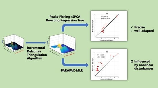
In recent years, optical methods have been proven to be a powerful tool for m onitoring dissolved organic carbon (DOC) in natural waters. However, the effectiveness of this method in marine systems with low DOC concentrations remains to be shown. Herein, a new method based on fluorescence excitation–emission matrix spectroscopy for seawater DOC quantification is proposed. Pre-processing method is investigated to achieve a high signal to noise ratio. Peak-picking operation is then performed to obtain feature peaks. In order to combine the information from sparsely located feature peaks, sparse principal component analysis is applied to identifying important variables used in the following regression procedure. Under these conditions the result of regression analysis can be obtained readily in a given data set coupling with boosting regression tree. The method was tested on samples collected from the East China Sea. Compared to the parallel factor analysis–multivariate linear regression method, experimental results show that the proposed method achieved a more consistent regression output and indicate that the boosting regression tree has potential for DOC quantification even at low concentrations.

1. Introduction

As an important carbon pool for oceans, dissolved organic carbon (DOC) has a critical role in global carbon cycle and provides a contribution to the carbon sequestration [1,2,3,4]. In addition, it is an important part of many trace elements in biogeochemistry [5,6,7], and therefore, the detection and monitoring of DOC is meaningful for the research of oceanic carbon cycle [4].

One of the general methods for DOC analysis in the ocean is the high-temperature catalytic oxidation (HTCO) method [8,9], which is utilized by many modern TOC analyzers. In this method, all carbon is oxidized to carbon dioxide, and total organic carbon is then evaluated by measuring the weight of carbon dioxide. However, this type of method requires high temperatures for combusting samples. In addition, a series of specialized instruments are needed to remove interferences, collect carbon dioxide and weight it. In practice, such an approach would be time consuming, and the equipment is costly. An alternative and as effective method is to monitor DOC with UV-visible spectroscopy [10,11], which establishes relationships between DOC quantity with spectral parameters such as the absorbance, peaks and slopes [12,13,14], without having to perform any chemical manipulations. This optical method can be useful for informative analysis and quantification. For example, absorbance at 254 nm is linked to aromatic humic substances [12,15] and is often used for dissolved organic carbon (DOC) [16]. At wavelengths 230 and 263 nm, there exist strong correlations between DOC and absorbance [17].

In addition to single wavelength methods, multiple wavelength methods based on empirical model are also useful in DOC quantification [18,19,20,21]. Causse et al. [11] used the second derivative values at 226 and 295 nm for nitrate and DOC measurement on small rivers of agricultural watershed. Carter et al. [16] divided UV spectra into strongly and weakly absorbing components. An unbiased prediction of DOC was obtained at wavelengths 270 and 350 nm. Fichot and Brenner [22] developed an approach by using the spectral slope coefficient for DOC estimation, which showed good performance in surface waters and coastal waters. In addition to widely used wavelengths 254 to 400 nm, Avagyan et al. [23] introduced 600 and 740 nm into DOC estimation. Combined with high-resolution absorbance method, it is a robust and simple method for DOC quantification. In most DOC quantification methods, UV spectra are often combined with molecular weight distributions [24,25,26,27,28], which is not rapid and presents relative few difficulties in the field. Although, some researchers have proposed some direct determination of DOC by using UV spectrophotometry [10,11], measured DOC concentrations must be higher than 5 mg/L. Considering the relatively low DOC concentration for the seawater samples, UV spectra methods are not sufficient.

Since fluorescence excitation−emission matrix spectroscopy has relatively higher sensitivity and selectivity compared with UV spectroscopy, it is increasingly used as a proxy indicator for DOC and water quality indicators [18,29,30,31]. Zhang et al. [31] applied self-organizing map (SOM) for pollution characterizing in fluorescence, then combined parallel factor analysis (PARAFAC) and regression method to predict the DOC concentration. Saraceno et al. [30] studied the relationship between DOC concentration and fluorescent dissolved organic matter (FDOM) in order to establish an accurate, high-resolution time series of DOC dynamics which can be useful during storm events.

Among the above methods proposed for DOC determination, however, there is little research about direct DOC quantification and the DOC of seawater. As DOC in seawater is now recognized as an important component of the biogeochemical system and possible indicator of global climate change [32], it is essential to monitor DOC easily and quickly. Thus, in this paper, a DOC quantification method based on fluorescence excitation–emission matrix spectroscopy is proposed. The proposed strategy includes three steps: surface smoothing, feature extraction and regression. This method was tested on seawater sampled from the East China Sea. A quantification performance of DOC concentration is shown on a testing data set.

2. Materials and Methods

2.1. Boosting Regression Tree Based Method

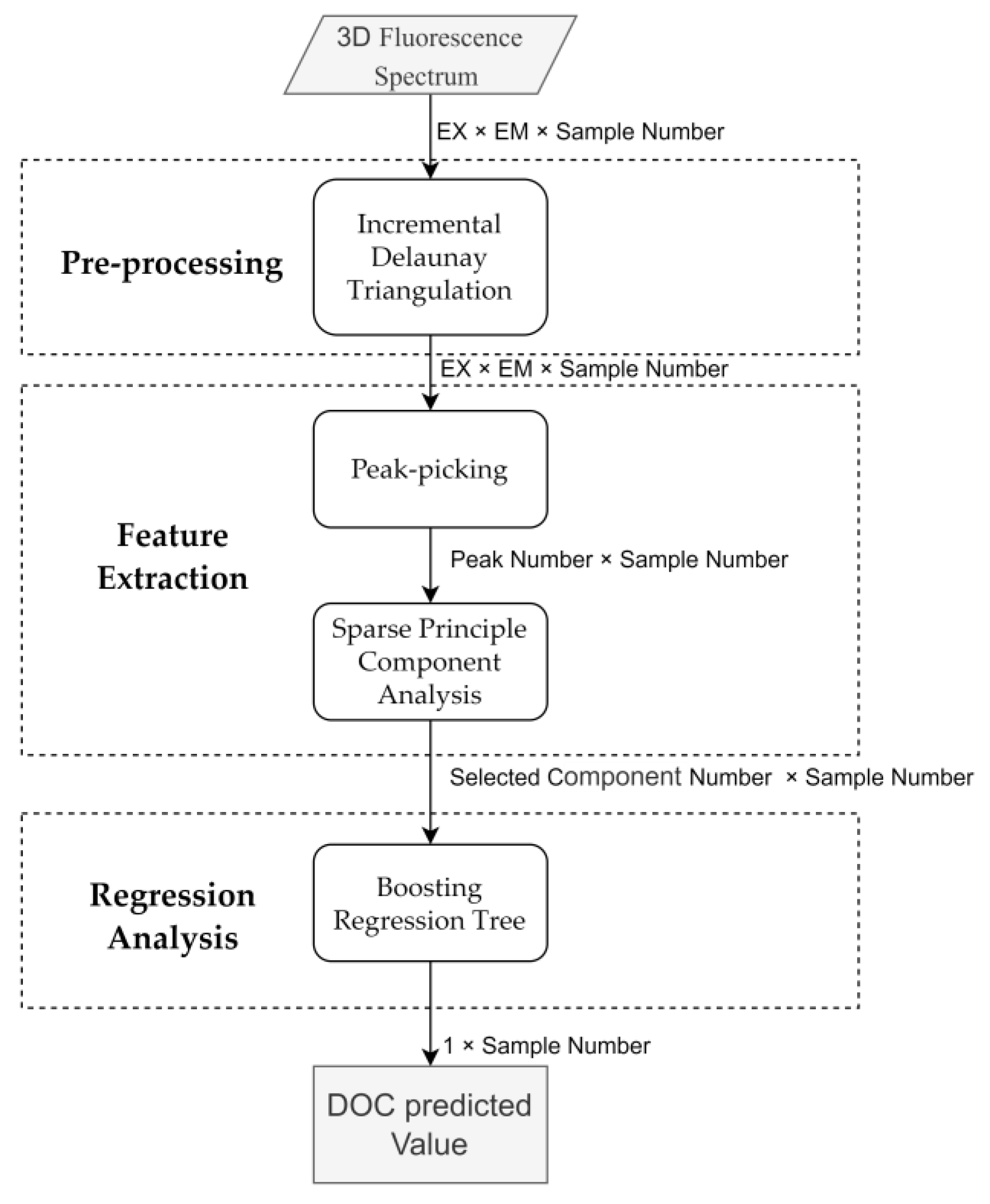
Pre-processing method based on incremental Delaunay triangulation algorithm is investigated to achieve a high signal to noise ratio. Feature extraction based on peak-picking operation and sparse principal component analysis is applied to identifying important variables used in the following regression procedure. The result of regression analysis can be obtained in a given data set coupling with boosting regression tree. The proposed method was shown in Figure 1, which included the principal method name and the data dimension after each procedure.

2.1.1. Incremental Delaunay Triangulation Algorithm

As there are Rayleigh and Raman scatter peaks which can create problems quantitative analysis, particularly for samples with low DOC concentrations, correction methods need be used to eliminate scatter peaks from fluorescence data. In this work, the scattering correction proposed by Zepp et al. [33] was adopted, which can excise scatter peaks efficiently. Although, three-dimensional interpolation was applied to this method, the remaining data still has low signal to noise ratio. There are ‘breaks’ or ‘peaks’ at connections of patches (triangle facets in Zepp et al. [33]). Therefore, results of scattering correction lack the surface continuity and smoothness, which may influence regression analysis.

In order to achieve some surface continuity and smoothing for EEMs data, a method termed incremental Delaunay triangulation [34,35] was utilized in this work. This algorithm inserts data points into the original matrix sequentially by selecting the most contribution subset from the matrix. The Delaunay triangulation is then used to approximate the elevation at subset points within a distant criterion. Based on the above operations, it is therefore relatively straight forward to obtain a continuous and smooth result.

2.1.2. Feature Extraction

In EEMs, not all of the fluorescence intensities have contribution to the final regression model. In this practical application, the fluorescence data should be preprocessed to transform them into new space of variables where, it is hoped, the goal of DOC quantification will be easier to achieve. Herein, this pre-processing stage utilized a peak-picking approach based on two-dimensional polynomial model and extremum detection. For a spectra matrix, a simple approximation to the plane is two-dimensional polynomial model:

$$D\left(x,y\right)=a{x}^2+b{y}^2+cxy+dx+ey+f$$

Then the sum of squared differences (SSD) is constructed:

$$\mathrm{SSD}={\displaystyle \sum }_{i=1}^n{[a{x}_i^2+b{y}_i^2+c{x}_i{y}_i+d{x}_i+e{y}_i+f-D\left(x_i,y_i\right)]}^2$$

The two-dimensional polynomial model that fits the plane best is the one with the lowest value of SSD. Thus, when SSD is differentiated with respect to parameters [a, …, f,] the values of different parameters can be got by solving:

$$\frac{d\mathrm{SSD}}{da}=0,\dots , \frac{d\mathrm{SSD}}{df}=0$$

To compute the $x$ and $y$ from function $D\left(x,y\right)$, we can differentiate $D\left(x,y\right)$ with respect to $x$ and $y$:

$$\frac{dD\left(x,y\right)}{dx}=0,\frac{dD\left(x,y\right)}{dy}=0$$

In this research, the peak-picking approach is not applied to the whole spectra matrix. In EEM data, the peaks are associated with phenol-like organic compounds, tryptophan-like, tyrosine-like, or humic-like [36]. Therefore, it can be divided into five regions: I, II, III, IV, and V. Then, the sparse principal component analysis is performed on these five EEM regions to get fluorescence peaks and their features. Having obtained the feature positions of the EEMs data, there remains the task of regression analysis with respect to DOC concentration.

2.1.3. Boosting Regression Tree

The boosting tree, based on additive model and forward stage-wise algorithm, is developed for regression and classification applications [37]. It produces competitive, highly robust, interpretable procedures, which is particularly appropriate for data with much disturbance. In this section, we review the basic boosting regression tree algorithm and then apply it on fluorescence spectroscopy.

Boosting regression tree given a training set $\left[\left({\mathit{x}}_1,y_1\right),\left({\mathit{x}}_2,y_2\right),\dots ,\left({\mathit{x}}_N,y_N\right)\right]$, with inputs ${\mathit{x}}_i\in {\mathit{R}}^N$ and outputs $y_i\in R$, the goal is to obtain a function estimation $f\left(\mathit{x}\right)$ that minimizes loss function $L\left(y,f\left(\mathit{x}\right)\right)$. Here, the boosting tree model is derived by assuming that the function estimation f(x) can be expressed as a sum of basic decision trees:

$$f_M\left(\mathit{x}\right)={\displaystyle \sum }_{m=1}^{M}T\left(\mathit{x};{\mathsf{\Theta }}_m\right)$$

where $T\left(\mathit{x};{\mathsf{\Theta }}_m\right)$ is the decision tree, ${\mathsf{\Theta }}_m$ is the parameter of the decision tree and $M$ is the number of trees. This boosting tree algorithm can be solved by using forward stagewise algorithm:

$$f_m\left(\mathit{x}\right)=f_{m-1}\left(\mathit{x}\right)+T\left(\mathit{x};{\mathsf{\Theta }}_m\right)$$

where $f_{m-1}\left(\mathit{x}\right)$ represents the current estimation model. The parameter ${\mathsf{\Theta }}_m$ of next decision tree can be determined by experiential risk minimization:

$${\mathsf{\Theta }}_m=\underset{{\mathsf{\Theta }}_m}{\mathrm{argmin}}{\displaystyle \sum }_{i=1}^{N}L\left(y_i,f_{m-1}\left({\mathit{x}}_i\right)+T\left({\mathit{x}}_i;{\mathsf{\Theta }}_m\right)\right)$$

A common choice of loss function in regression problems is the squared loss given by:

$$L\left(y,f_{m-1}\left(\mathit{x}\right)+T\left(\mathit{x};{\mathsf{\Theta }}_m\right)\right)=\left[y-f_{m-1}\left(\mathit{x}\right)-T\left(\mathit{x};{\mathsf{\Theta }}_m\right){]}^2=\right[r-T\left(\mathit{x};{\mathsf{\Theta }}_m\right){]}^2$$

where $r=y-f_{m-1}\left(\mathit{x}\right)$. In this case, $r$ is the residual of the regression model. Therefore, our goal is to choose appropriate regression tree model $T\left(\mathit{x};{\mathsf{\Theta }}_m\right)$ so as to fitting the residual $r-T\left(\mathit{x};{\mathsf{\Theta }}_m\right)$.

In the case of the fluorescence data, single EEM data $\mathit{X}$ is divided into 5 regions. A single EEM data is therefore represented by a $5$-dimensional vector, each point of which represents a single fluorescence intensity corresponding to the concentration of dissolved organic carbon. The training data set was used to construct a boosting regression tree, and then the testing data set will be used to evaluate the regression model.

2.2. PARAFAC-MLR Model

PARAFAC [38,39] is one of several methods that has been successfully applied on analysis of fluorescence data. Considering a three-way array given by three loading matrices, $\mathit{A}\in {\mathit{R}}^{I\times F}$, $\mathit{B}\in {\mathit{R}}^{J\times F}$, and $\mathit{C}\in {\mathit{R}}^{K\times F}$, with elements $a_{if}$, $b_{jf}$, and $a_{kf}$, in which each element can be expressed as

$$x_{ijk}={\displaystyle \sum }_{f=1}^F{a}_{if}{b}_{jf}{c}_{kf}+e_{ijk},i=1\cdots I,j=1\cdots J,k=1\cdots K$$

where $e_{ijk}$ are the residuals and $F$ is the number of sought factors [40]. By employing the Khatri–Rao product ⨀, the three-way array can be represented as a two-way array which is composed of several matrices:

$$X=\mathit{A}{(\mathit{C}\odot \mathit{B})}^T+\mathit{E}$$

Then it minimizes the following three loss functions with alternating least squares method:

$${\sigma }_1=\Vert {\mathit{X}}^{I\times JK}-\mathit{A}{(\mathit{C}\odot \mathit{B})}^T{\Vert }_F^2$$

$${\sigma }_2=\Vert {\mathit{X}}^{J\times KI}-\mathit{B}{(\mathit{A}\odot \mathit{C})}^T{\Vert }_F^2$$

$${\sigma }_3=\Vert {\mathit{X}}^{K\times JI}-\mathit{C}{(\mathit{B}\odot \mathit{A})}^T{\Vert }_F^2$$

where $F$ is the Frobenius norm. The score vector $\mathit{C}$ is then combined with MLR method to define a regression model. Such a model can directly accommodate multiple predictors, and it is possible to have an observation that is well within the range of each individual predictor values.

2.3. Assessing the Accuracy of the Model

It is natural to want to quantify the extent to which the model fits the data. The $R^2$ statistic provides an alternative measure of the quality of a linear regression fit [41]. It takes the form of a proportion, assuming a value between 0 and 1.

$$R^2=1-\frac{{{\displaystyle \sum }}^{ }{({\mathrm{DOC}}_{pre}-{\mathrm{DOC}}_{real})}^2}{{{\displaystyle \sum }}^{ }{\mathrm{DOC}}_{real}{}^2}$$

where ${\mathrm{DOC}}_{pre}$ is the predicted value of DOC and ${\mathrm{DOC}}_{real}$ is the real value of DOC. Hence, the $R^2$ statistic measures the proportion of variability in DOC that can be explained using fluorescence data.

2.4. Experiment

2.4.1. Site Descriptions and Sampling

Seawater samples for this investigation were taken from the coastal water in East China Sea. The annual average temperature here is 16 °C and the annual precipitation is 927~1620 mm. Seawater samples were collected in 500 mL amber laboratory bottle and filtered through 0.45 mm cellulose nitrate membrane filters. As all these seawater samples were analyzed in the laboratory, filtered samples were stored in a fridge at 4 °C for several days. Low temperature can inhibit the activity of undesirable microorganisms and slow down chemical reaction rate. Sixty seawater samples were taken from nine different sample points. In order to obtain a gradient in concentration simulating the DOC of seawater far away from land, the samples at each point were diluted with pure water.

2.4.2. Fluorescence Measurements

Water samples were allowed to warm to room temperature prior to fluorescence measurements. The fluorescence measurements of seawater samples were performed using a F-7000 Fluorescence Spectrophotometer (Hitachi, Tokyo, Japan) and a quartz cuvette with 1 cm path length. The excitation wavelength ranged from 200 nm to 700 nm with a 5 nm interval, and the emission wavelength ranged from 200 nm to 700 nm with a 5 nm interval as well. According to the common regions of fluorescence maxima [42], the fluorescence for analysis has the excitation wavelength region of 200~360 nm and emission wavelength region of 275~460 nm.

All calculations were carried out on a personal computer equipped with a Core i7 2.5 GHz processor with 16 GB RAM under Windows 10 operating system using MATLAB R2016a (MathWorks, Natick, MA, USA).

2.4.3. DOC Measurements

The concentration of dissolved organic carbon was analyzed with TOC-L CPN (Shimadzu, Japan), which adopts the 680 °C combustion catalytic oxidation method. Sample acidification and sparging with purified air were carried out automatically. Because of the automatic dilution function, it has a wide measurement range of 4 μg/L to 30,000 mg/L.

3. Results

3.1. Pre-Processing

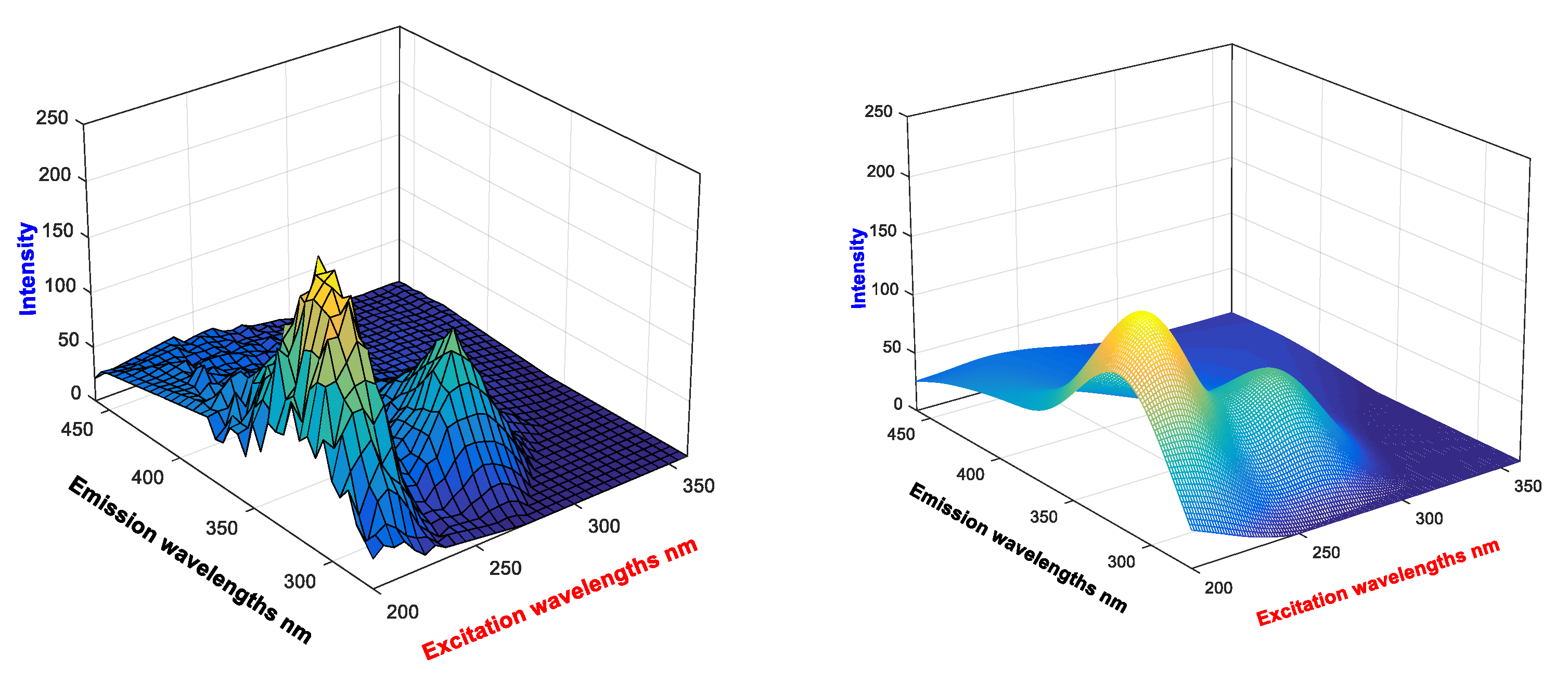
Illustration of the effects of incremental Delaunay triangulation pre-processing applied to the EEMs data set is shown in Figure 2. The plot on the left shows the original data (after scattering correction). The plot on the right shows the result of the surface-smoothing operation of the data. As shown, the fluorescence data resulting from scattering correction is a noisy data set, thus feature extraction depending on feature peaks cannot be applied. However, incremental Delaunay triangulation algorithm provides smooth surfaces and leads to a higher signal to noise ratio.

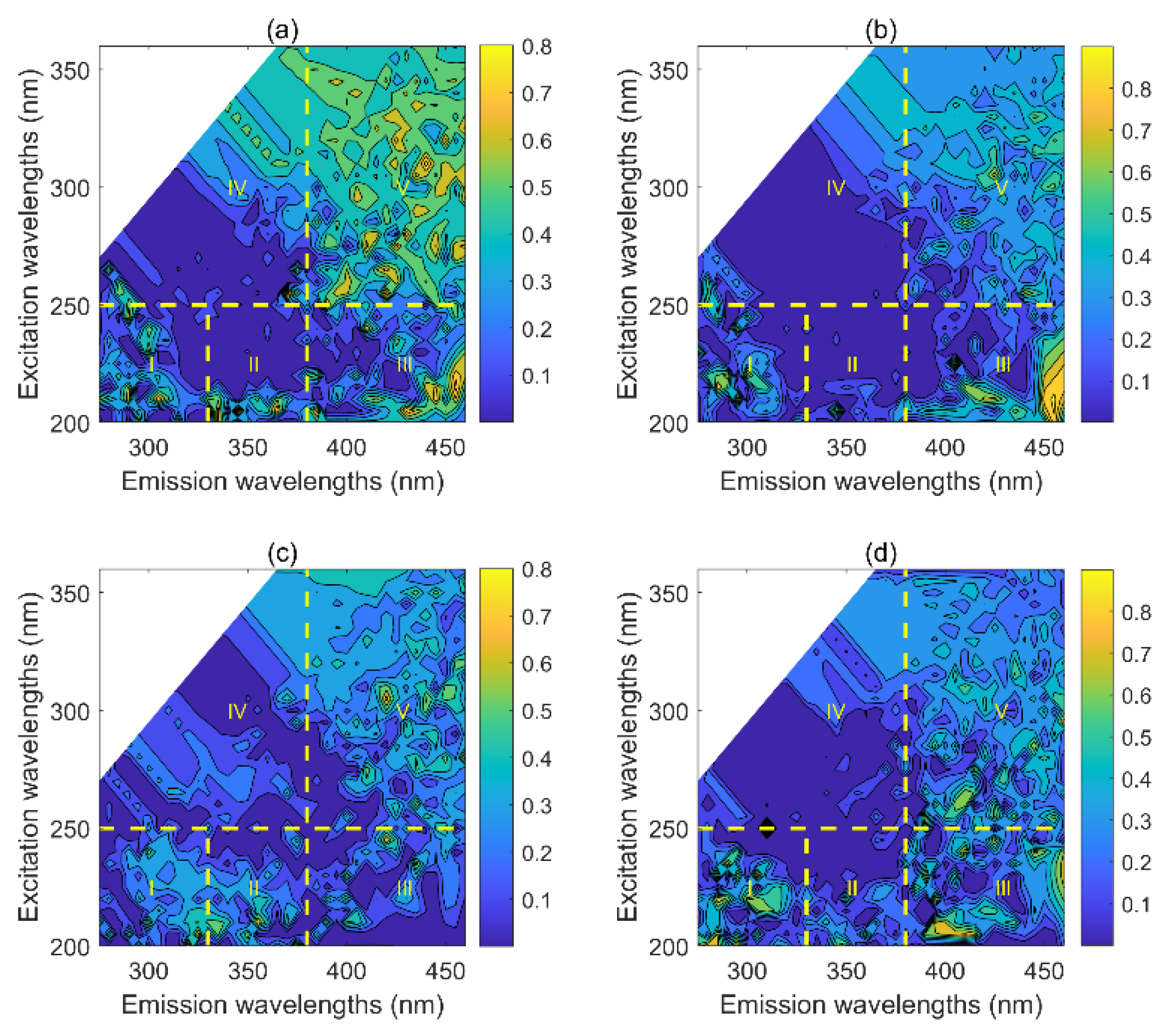
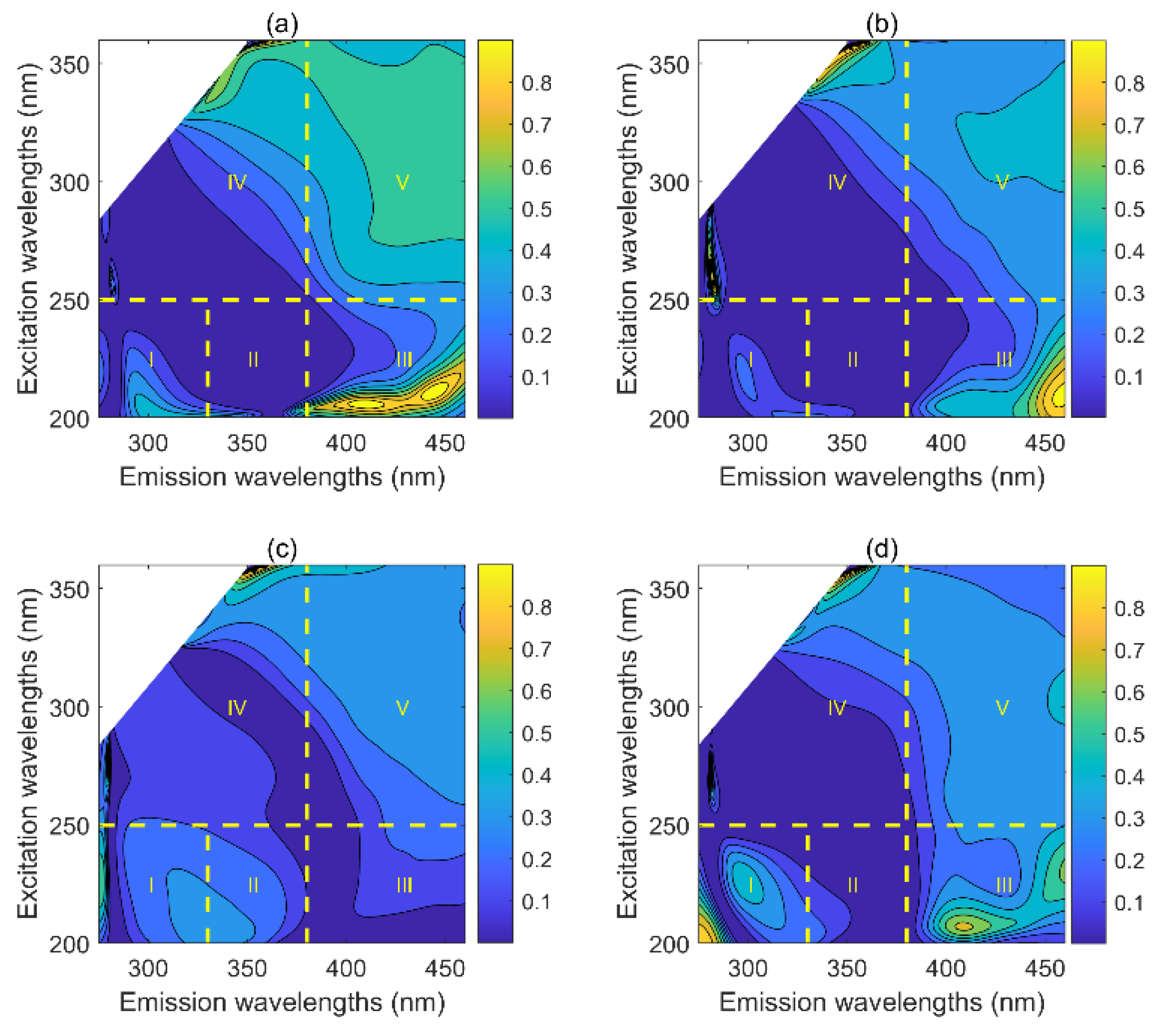
Furthermore, the R-square statistic between fluorescence intensities of EEM data and measured DOC concentration was analyzed directly to estimate the effectiveness of pre-processing results as indicators for DOC concentration. Figure 3 and Figure 4 showed the four contour plots of R-square statistic for regression analysis. As shown in this figure, horizontal and vertical lines were drawn to divide the EEM into five regions [28,43]. For EEM Region I and Region II, which are related to tyrosine protein-like matter, the emission wavelengths are shorter than 350 nm and excitation wavelengths are shorter than 250 nm. The location of Region III has the emission wavelengths longer than 350 nm and excitation wavelengths shorter than 250 nm, which represents the fulvic acid-like matter. Region IV are assigned to soluble microbial by-product-like matter. It is located at the emission wavelengths (<380 nm) with excitation wavelengths ranged from 250 to 280 nm. Excitation wavelengths shorter than 280 nm and emission wavelengths longer than 380 nm are defined as Region V. This region indicates the property of humic acid-like organics.

In Figure 3, data points that have the strongest correlations between EEM and DOC concentrations are scattered in fluorescence matrix only in regions clustering together. Because there are peaks caused by noise, it may have negative influences on later regression analysis. Therefore, theoretically, information in the fluorescence can be barely detected, which results in substantially lower signal to noise ratio. Conversely, for EEMs data with smoothing in Figure 4, most of data points that have the strongest correlations between EEM, and DOC concentrations clustered together. The feature peaks with high value of R² therefore can be well extracted and make contribution to regression analysis.

3.2. Boosting Regression Tree Approach

To illustrate the performance of these two DOC quantification methods, among 60 samples were collected, 30 samples are specified as testing data chosen randomly, while 30 samples are used for training. On each of these training sets, boosting regression tree and PARAFAC-MLR approaches were fitted to the data and computed the resulting test error rate on a test set. The DOC concentrations of training set ranged from 0.7128 to 5.6290 mg/L, while the testing set ranged from 1.7500 to 5.6650 mg/L. The $R^2$ statistic and mean square error (MSE) is computed, which can measure the model fitting and explain the fraction of variance.

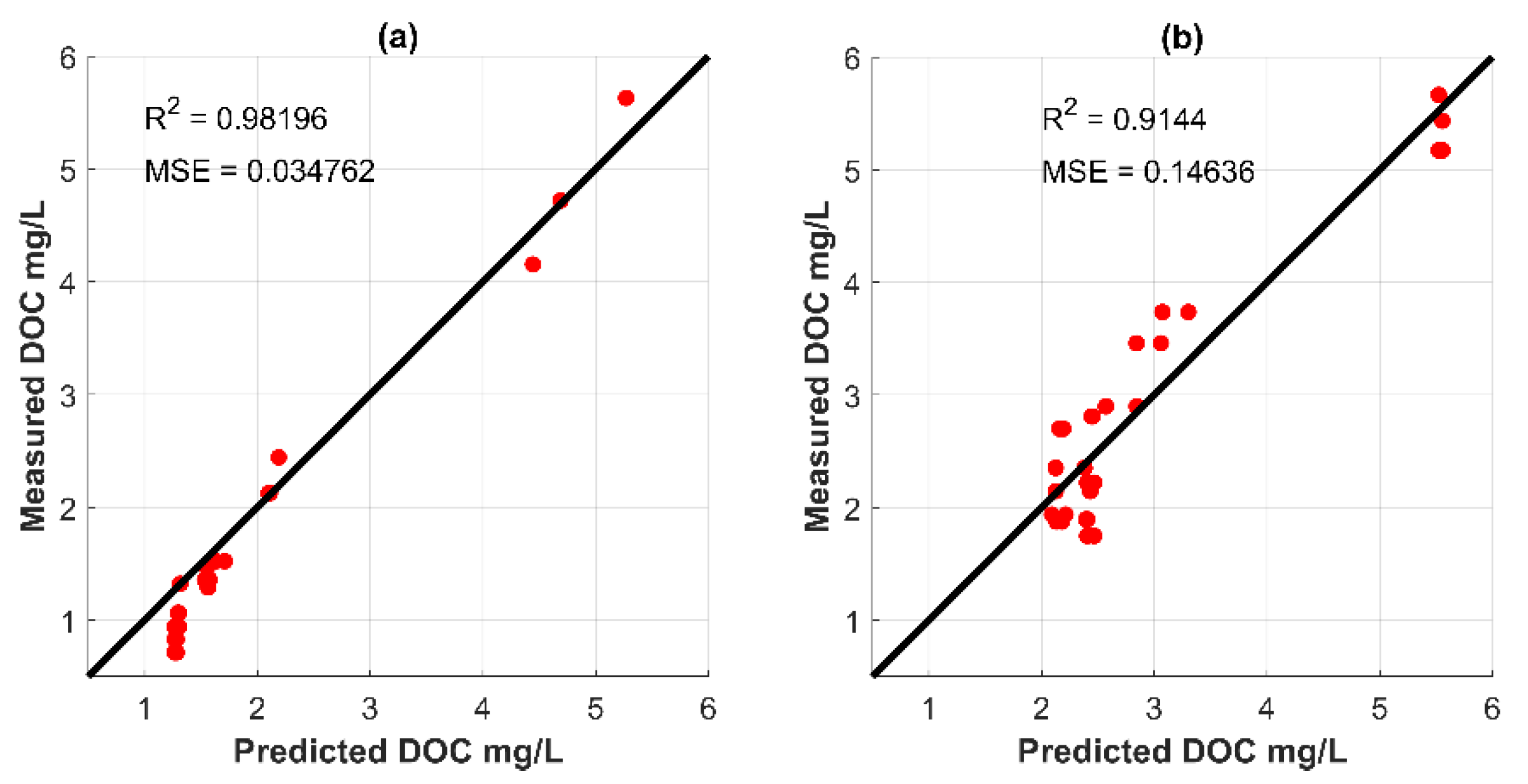
As shown in Figure 5a, the relationship of predicted and measured DOC is plotted. Predicted DOC concentrations ranged from 1.2683 to 5.2708 mg/L. $R^2$ is equal to 0.982 and MSE is 0.003, which indicates that the boosting regression tree almost describes the whole variance in the training data set. As shown in above (Section 2.1), the boosting regression tree fits a decision to the residual from the model. At each step, a new decision tree is added into the fit function in order to fit the residual from previously grown trees. Thus, the residual error of the regression model is driven to zero.

The relationship of predicted and measured DOC is plotted in Figure 5b. In Figure 5b, the model trained with training data was applied to the testing data set. Predicted DOC concentrations ranged 2.0919 to 5.5083 mg/L, the $R^2$ statistic of the boosting regression tree model, which gives a measure of the linear relationship between measured and predicted DOC concentrations. The $R^2$ was 0.914, and so 91.4% of the measured DOC concentrations is predicted by the boosting regression tree. The MSE is 0.146, which indicates that the predicted DOC concentrations are close to the measured DOC concentrations.

3.3. PARAFAC-MLR Approach

For PARAFAC-MLR quantification method, the procedure is quite different from the boosting regression tree. This difference stems from the fact that in the PARAFAC quantification case, the samples to be predicted need to be analyzed with measured samples. As the three-way array was decomposed into one score vector and two loading vectors, the concentration of the analytes was estimated using score vector, which represents the relative concentration of each sample. However, the score vector is, in fact, a $N\times F$ matrix, which leads to some difficulties for regression analysis. Here, an alternative is to introduce multivariable linear regression. Therefore, the DOC concentrations of seawater samples can be obtained according to the score vector of PARAFAC solution combined with multivariable linear regression.

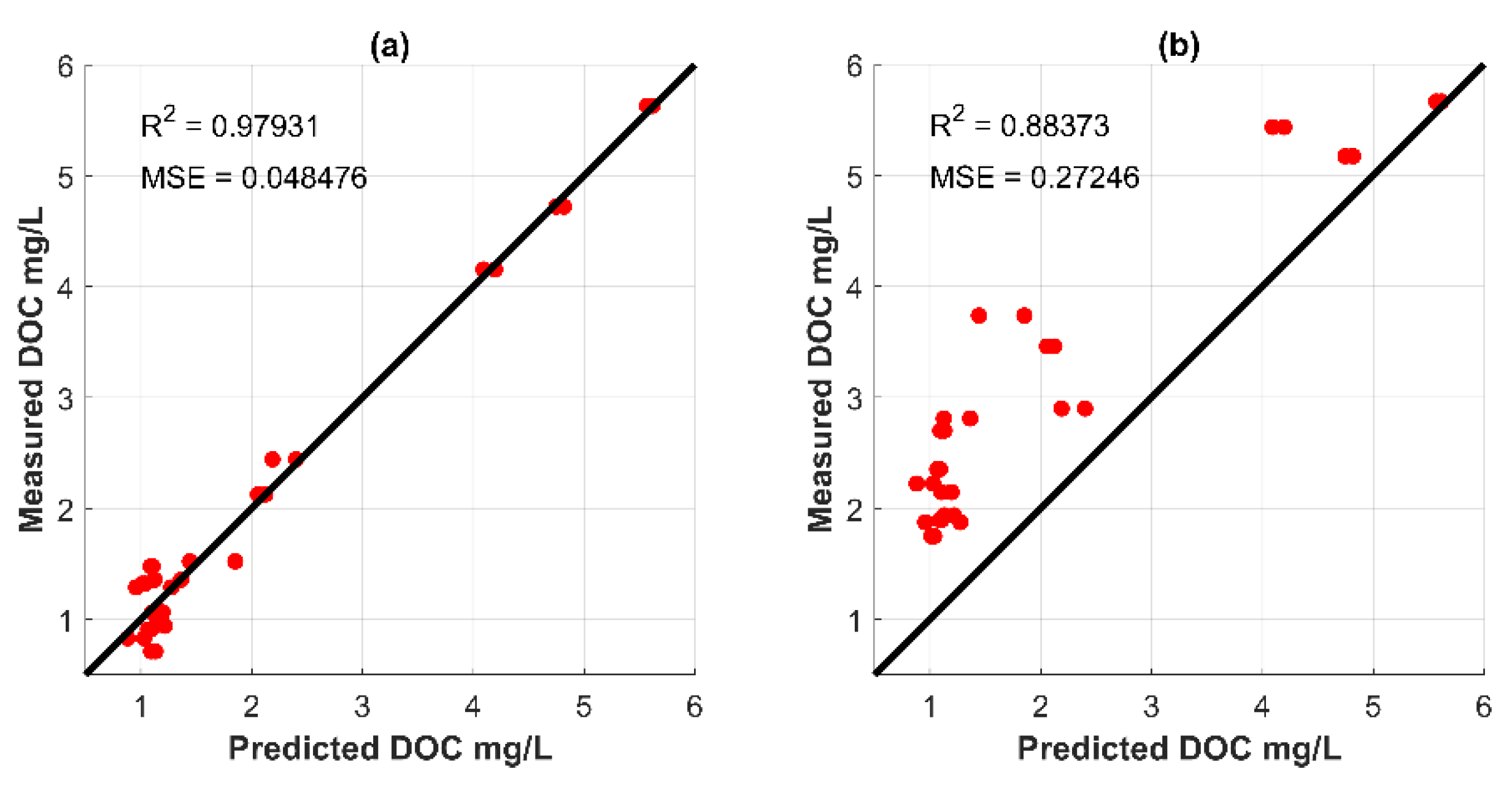
In this work, PARAFAC is based on N-way toolbox [44], which is freely downloadable from the Chemometrics site at University of Copenhagen (www.models.life.ku.dk, accessed on 6 October 2021). The PARAFAC-MLR result of training data set is shown in Figure 6a. In this example, the $R^2$ value over training data is 0.979 and MSE is 0.05, which means the PARAFAC-MLR provides a good fit to the training data.

Figure 6b provides the results of PARAFAC decomposition and predicted result of DOC concentrations are shown in. Notice that the value of $R^2$ statistic is 0.884, which indicates the measured values, and the predicted values are near linear. However, because the MSE is 0.272, it indicates that the PARAFAC-MLR model does not fit the testing data consistently. Since the success of PARAFAC decomposition is dependent on signal-to-noise ratio [45,46], the regression results suffer from limitations because of the possible noisy, nonlinear disturbances. All these factors can lead to a poor fit to the data set. Therefore, the PARAFAC-MLR method should be further optimized when applied for predicting DOC concentrations.

4. Discussion

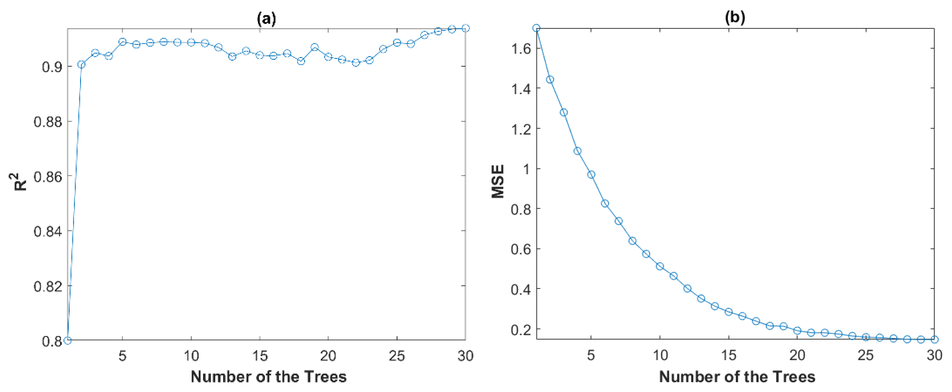
The difference between these two results can be understood by noting that there is considerable amount of information presented by EEM. In general, the PARAFAC-MLR method is a comprehensive indicator of concentration measurement. As it offers a useful but not sufficient concentration analysis, there needs to be a feature extraction which is essential pre-processing step to data analysis. Feature extraction can greatly reduce noise disturbances and make it much easier for a subsequent regression analysis. In addition, as shown in Figure 5b or Figure 6b, PARAFAC-MLR performs less efficiently than the proposed method because MLR is designed for linear situations. In a real-life situation in which the true relationship is unknown, the boosting tree-based method may still provide better results to MLR whether the true relationship is linear or non-linear. In particular, instead of fitting a linear regression model for loading matrix, boosting regression tree provides an improvement over PARAFAC-MLR method in regression analysis. As in this tree method, a number of decision trees are built based on the bootstrapped EEM samples. Then the training samples are separately fitted to different trees. Finally, all these trees will be combined into a decision model. In Figure 7, with the number of trees increased, R-square in Figure 7a changed and the mean squared error (MSE) in Figure 7b decreased. This indicates that boosting regression tree method utilizes the information of fluorescence intensities at different regions and tries to integrate information by discovering and identifying mappings between different decision trees. In Figure 7a, R-square grew rapidly from 1 to 2 because simple tree models are very restricted in term of the data relationship that they can represent. Moreover, R-square firstly decreased and then increased from 10 to 25, which means that the proposed boosting regression tree was able to find better predicted value. Empirically, this ensemble method which uses multiple models tends to yield better results.

Although, when applied correctly, boosting regression tree method can provide a relatively sufficient analysis of DOC concentration in fluorescence data, it is not always suitable. The samples with large biases can have a significant impact on the accuracy of the regression model. Because boosting method will highlight bias, samples with large biases will influence the weights among decision trees, which may yield unsatisfactory prediction results. In practice these issues are unavoidable but with increasing number of input data points they have less impact.

5. Conclusions

Dissolved organic matter (DOC) has a relatively important role for carbon cycle and linking the marine carbon cycle to climate [47,48]. The development of an inexpensive and fast quantitative procedure for DOC is meaningful for real practice. This paper described a new, quantitative method for DOC in seawater by fluorescence excitation–emission matrix spectroscopy. Samples collected from the East China Sea were analyzed with fluorescence spectroscopy at laboratory. Incremental Delaunay triangulation algorithms ensure that patches are continuous at the connections, thus it can provide smooth surfaces. Moreover, a peak-picking method for EEMs data was applied to identify the local maxima. However, the result of peak detection is sparse and not computationally efficient. In this work, sparse principal component analysis was used to achieve dimensionality reduction, which has the advantage of identifying important variables.

For the regression analysis in this study, a mapping model between DOC concentrations and fluorescence intensities of EEM were established on the basis of boosting regression tree method. The comparison with PARAFAC method further indicates that boosting regression tree provided a better performance at DOC estimation. The correlations between DOC concentrations and fluorescence EEM suggested that fluorescence spectroscopy has a potential for estimating the DOC concentrations of seawater. This emerging set of different fluorescence intensities can help in creating a common method for the DOC quantification.

References

- Williams, P.M.; Druffel, E.R.M. Radiocarbon in dissolved organic matter in the central North Pacific Ocean. Nat. Cell Biol. 1987, 330, 246–248. [Google Scholar] [CrossRef] [Green Version]
- Santinelli, C.; Ribotti, A.; Sorgente, R.; Gasparini, G.; Nannicini, L.; Vignudelli, S.; Seritti, A. Coastal dynamics and dissolved organic carbon in the western Sardinian shelf (Western Mediterranean). J. Mar. Syst. 2008, 74, 167–188. [Google Scholar] [CrossRef]
- Hansell, D.A.; Carlson, C.A. Deep-ocean gradients in the concentration of dissolved organic carbon. Nat. Cell Biol. 1998, 395, 263–266. [Google Scholar] [CrossRef]
- Avril, B. DOC dynamics in the northwestern Mediterranean Sea (DYFAMED site). Deep. Sea Res. Part II Top. Stud. Oceanogr. 2002, 49, 2163–2182. [Google Scholar] [CrossRef]
- Guo, L.; Santschi, P.H. Sedimentary sources of old high molecular weight dissolved organic carbon from the ocean margin benthic nepheloid layer. Geochim. Cosmochim. Acta 2000, 64, 651–660. [Google Scholar] [CrossRef]
- Rue, E.L.; Bruland, K.W. The role of organic complexation on ambient iron chemistry in the equatorial Pacific Ocean and the response of a mesoscale iron addition experiment. Limnol. Oceanogr. 1997, 42, 901–910. [Google Scholar] [CrossRef] [Green Version]
- Coale, K.H.; Bruland, K.W. Copper complexation in the Northeast Pacific. Limnol. Oceanogr. 1988, 33, 1084–1101. [Google Scholar] [CrossRef]
- Sharp, J.H.; Benner, R.; Bennett, L.; Carlson, C.A.; Fitzwater, S.E.; Peltzer, E.; Tupas, L.M. Analyses of dissolved organic carbon in seawater: The JGOFS EqPac methods comparison. Mar. Chem. 1995, 48, 91–108. [Google Scholar] [CrossRef]
- Sharp, J.H. Marine dissolved organic carbon: Are the older values correct? Mar. Chem. 1997, 56, 265–277. [Google Scholar] [CrossRef]
- Cook, S.; Peacock, M.; Evans, C.D.; Page, S.E.; Whelan, M.J.; Gauci, V.; Kho, L.K. Quantifying tropical peatland dissolved organic carbon (DOC) using UV-visible spectroscopy. Water Res. 2017, 115, 229–235. [Google Scholar] [CrossRef] [Green Version]
- Causse, J.; Thomas, O.; Jung, A.-V.; Thomas, M.-F. Direct DOC and nitrate determination in water using dual pathlength and second derivative UV spectro-photometry. Water Res. 2017, 108, 312–319. [Google Scholar] [CrossRef]
- Weishaar, J.L.; Aiken, G.R.; Bergamaschi, B.; Fram, M.; Fujii, R.; Mopper, K. Evaluation of Specific Ultraviolet Absorbance as an Indicator of the Chemical Composition and Reactivity of Dissolved Organic Carbon. Environ. Sci. Technol. 2003, 37, 4702–4708. [Google Scholar] [CrossRef]
- Spencer, R.G.M.; Butler, K.D.; Aiken, G.R. Dissolved organic carbon and chromophoric dissolved organic matter properties of rivers in the USA. J. Geophys. Res. Space Phys. 2012, 117, 1–14. [Google Scholar] [CrossRef]
- Peuravuori, J.; Pihlaja, K. Molecular size distribution and spectroscopic properties of aquatic humic substances. Anal. Chim. Acta 1997, 337, 133–149. [Google Scholar] [CrossRef]
- Edzwald, J.K.; Becker, W.C.; Wattier, K.L. Surrogate Parameters for Monitoring Organic Matter and THM Precursors. J. Am. Water Work. Assoc. 1985, 77, 122–132. [Google Scholar] [CrossRef]
- Carter, H.T.; Tipping, E.; Koprivnjak, J.-F.; Miller, M.; Cookson, B.; Hamilton-Taylor, J. Freshwater DOM quantity and quality from a two-component model of UV absorbance. Water Res. 2012, 46, 4532–4542. [Google Scholar] [CrossRef] [Green Version]
- Peacock, M.; Evans, C.D.; Fenner, N.; Freeman, C.; Gough, R.; Jones, T.G.; Lebron, I. UV-visible absorbance spectroscopy as a proxy for peatland dissolved organic carbon (DOC) quantity and quality: Considerations on wavelength and absorbance degradation. Environ. Sci. Process. Impacts 2014, 16, 1445–1461. [Google Scholar] [CrossRef] [Green Version]
- Downing, B.D.; Boss, E.; Bergamaschi, B.A.; Fleck, J.A.; Lionberger, M.A.; Ganju, N.K.; Schoellhamer, D.H.; Fujii, R. Quantifying fluxes and characterizing compositional changes of dissolved organic matter in aquatic systems in situ using combined acoustic and optical measurements. Limnol. Oceanogr. Methods 2009, 7, 119–131. [Google Scholar] [CrossRef] [Green Version]
- Tipping, E.; Corbishley, H.T.; Koprivnjak, J.-F.; Lapworth, D.J.; Miller, M.P.; Vincent, C.D.; Hamilton-Taylor, J. Quantification of natural DOM from UV absorption at two wavelengths. Environ. Chem. 2009, 6, 472–476. [Google Scholar] [CrossRef] [Green Version]
- Asmala, E.; Stedmon, C.; Thomas, D. Linking CDOM spectral absorption to dissolved organic carbon concentrations and loadings in boreal estuaries. Estuar. Coast. Shelf Sci. 2012, 111, 107–117. [Google Scholar] [CrossRef]
- Wang, G.-S.; Hsieh, S.-T. Monitoring natural organic matter in water with scanning spectrophotometer. Environ. Int. 2001, 26, 205–212. [Google Scholar] [CrossRef]
- Fichot, C.G.; Benner, R. A novel method to estimate DOC concentrations from CDOM absorption coefficients in coastal waters. Geophys. Res. Lett. 2011, 38. [Google Scholar] [CrossRef]
- Avagyan, A.; Runkle, B.R.K.; Kutzbach, L. Application of high-resolution spectral absorbance measurements to determine dissolved organic carbon concentration in remote areas. J. Hydrol. 2014, 517, 435–446. [Google Scholar] [CrossRef] [Green Version]
- Her, N.; Amy, G.; Foss, D.; Cho, J. Variations of Molecular Weight Estimation by HP-Size Exclusion Chromatography with UVA versus Online DOC Detection. Environ. Sci. Technol. 2002, 36, 3393–3399. [Google Scholar] [CrossRef] [PubMed]
- Korshin, G.; Benjamin, M.M.; Sletten, R.S. Adsorption of natural organic matter (NOM) on iron oxide: Effects on NOM composition and formation of organo-halide compounds during chlorination. Water Res. 1997, 31, 1643–1650. [Google Scholar] [CrossRef]
- Leenheer, J.A.; Croué, J.-P. Peer Reviewed: Characterizing Aquatic Dissolved Organic Matter. Environ. Sci. Technol. 2003, 37, 18A–26A. [Google Scholar] [CrossRef] [Green Version]
- Perminova, I.V.; Frimmel, F.H.; Kudryavtsev, A.V.; Kulikova, N.A.; Abbt-Braun, G.; Hesse, S.; Petrosyan, V.S. Molecular Weight Characteristics of Humic Substances from Different Environments as Determined by Size Exclusion Chromatography and Their Statistical Evaluation. Environ. Sci. Technol. 2003, 37, 2477–2485. [Google Scholar] [CrossRef]
- Xiao, K.; Sun, J.-Y.; Shen, Y.-X.; Liang, S.; Liang, P.; Wang, X.-M.; Huang, X. Fluorescence properties of dissolved organic matter as a function of hydrophobicity and molecular weight: Case studies from two membrane bioreactors and an oxidation ditch. Rsc Adv. 2016, 6, 24050–24059. [Google Scholar] [CrossRef]
- Belzile, C.; Roesler, C.S.; Christensen, J.P.; Shakhova, N.; Semiletov, I. Fluorescence measured using the WETStar DOM fluorometer as a proxy for dissolved matter absorption. Estuar. Coast. Shelf Sci. 2006, 67, 441–449. [Google Scholar] [CrossRef]
- Saraceno, J.F.; Pellerin, B.A.; Downing, B.D.; Boss, E.; Bachand, P.A.M.; Bergamaschi, B.A. High-frequency in situ optical measurements during a storm event: Assessing relationships between dis-solved organic matter, sediment concentrations, and hydrologic processes. J. Geophys. Res. 2009, 114. [Google Scholar] [CrossRef]
- Zhang, Y.; Liang, X.; Wang, Z.; Xu, L. A novel approach combining self-organizing map and parallel factor analysis for monitoring water quality of watersheds under non-point source pollution. Sci. Rep. 2015, 5, 16079. [Google Scholar] [CrossRef] [Green Version]
- Church, M.J.; Ducklow, H.W.; Karl, D.M. Multiyear increases in dissolved organic matter inventories at Station ALOHA in the North Pacific Subtropical Gyre. Limnol. Oceanogr. 2002, 47, 1–10. [Google Scholar] [CrossRef] [Green Version]
- Zepp, R.G.; Sheldon, W.M.; Moran, M.A. Dissolved organic fluorophores in southeastern US coastal waters: Correction method for eliminating Rayleigh and Raman scattering peaks in excitation–emission matrices. Mar. Chem. 2004, 89, 15–36. [Google Scholar] [CrossRef]
- Soommart, S.; Paitoonwattanakij, K. Incremental Delaunay triangulation algorithm for digital terrain modelling. Thammasat Int. J. Sci. Tech. 1999, 4, 64–75. [Google Scholar]
- Sakhi, A.; Naimi, B. A hybrid refinement/decimation triangulation method for image approximation. In Proceedings of the 5th International Conference on Visual Information Engineering (VIE 2008), Xi’an, China, 29 July–1 August 2008. [Google Scholar]
- Chen, W.; Westerhoff, P.; Leenheer, J.A.; Booksh, K. Fluorescence excitation—emission matrix regional integration to quantify spectra for dissolved organic matter. Environ. Sci. Technol. 2003, 37, 5701–5710. [Google Scholar] [CrossRef]
- Friedman, J.H. Greedy function approximation: A gradient boosting machine. Ann. Stat. 2001, 29, 1189–1232. [Google Scholar] [CrossRef]
- Bro, R. PARAFAC. Tutorial and applications. Chemom. Intell. Lab. Syst. 1997, 38, 149–171. [Google Scholar] [CrossRef]
- Bro, R. Multi-Way Analysis in the Food Industry-Models, Algorithms, and Applications. 1998. Available online: https://www.semanticscholar.org/paper/MULTI-WAY-ANALYSIS-IN-THE-FOOD-INDUSTRY-Models%2C-%26-Bro/f2bdc868e33937a52c519bdf13e51a7afffbc03c#citing-papers (accessed on 6 October 2021).
- Tomasi, G.; Bro, R. PARAFAC and missing values. Chemom. Intell. Lab. Syst. 2005, 75, 163–180. [Google Scholar] [CrossRef]
- James, G.; Witten, D.; Hastie, T.; Tibshirani, R. An Introduction to Statistical Learning; Springer: New York, NY, USA, 2013; Volume 103. [Google Scholar]
- Coble, P.G. Marine optical biogeochemistry: The chemistry of ocean color. Chem. Rev. 2007, 107, 402–418. [Google Scholar] [CrossRef]
- Chen, R.; Ren, L.-F.; Shao, J.; He, Y.; Zhang, X. Changes in degrading ability, populations and metabolism of microbes in activated sludge in the treatment of phenol wastewater. RSC Adv. 2017, 7, 52841–52851. [Google Scholar] [CrossRef] [Green Version]
- Andersson, A.C.; Bro, R. The N-way Toolbox for MATLAB. Chemom. Intell. Lab. Syst. 2000, 52, 1–4. [Google Scholar] [CrossRef]
- Bro, R.; Jong, S.D. A fast non-negativity-constrained least squares algorithm. J. Chemom. 1997, 11, 393–401. [Google Scholar] [CrossRef]
- Bro, R.; Sidiropoulos, N.D. Least squares algorithms under unimodality and non-negativity constraints. J. Chemom 1998, 12, 223–247. [Google Scholar] [CrossRef]
- Hansell, D.A.; Carlson, C.A. Biogeochemistry of Marine Dissolved Organic Matter; Academic Press: Cambridge, MA, USA, 2014. [Google Scholar]
- Yang, Y.Z.; Peleato, N.M.; Legge, R.L.; Andrews, R.C. Fluorescence excitation emission matrices for rapid detection of poly-cyclic aromatic hydrocarbons and pesticides in surface waters. Environ. Sci. Water Res. Technol. 2019, 5, 315–324. [Google Scholar] [CrossRef]
Figure 1.
Flow chart diagram of proposed method.
Figure 2.
Comparison of scatter-corrected EEMs (original) and surface-smoothed EEMs (pre-processed).
Figure 3.
Contour plots of R-square statistic for regression analysis between DOC concentration and EEMs data of undiluted actual seawater without smoothing, (a–d) is the sample from different typical sample point.
Figure 4.
Contour plots of R-square statistic for regression analysis between DOC concentration and EEMs data of undiluted actual seawater after smoothing, (a–d) is the sample from different typical sample point, same as Figure 3.
Figure 5.
Regression results from performing boosting regression tree for the DOC training (a) and testing (b) data set.
Figure 6.
Regression results from performing PARAFAC-MLR for the DOC training (a) and testing (b) data set.
Figure 7.
(a) and mean squared error (MSE) (b) results from performing boosting regression tree on testing data set.
Publisher’s Note: MDPI stays neutral with regard to jurisdictional claims in published maps and institutional affiliations. |
© 2021 by the authors. Licensee MDPI, Basel, Switzerland. This article is an open access article distributed under the terms and conditions of the Creative Commons Attribution (CC BY) license (https://creativecommons.org/licenses/by/4.0/).
Share and Cite
MDPI and ACS Style
Yin, H.; Wang, K.; Liu, Y.; Huang, P.; Yu, J.; Hou, D. Fluorescence Excitation–Emission Matrix Spectroscopy and Boosting Regression Tree Model to Detect Dissolved Organic Carbon in Water. Water 2021, 13, 3612. https://doi.org/10.3390/w13243612
AMA Style
Yin H, Wang K, Liu Y, Huang P, Yu J, Hou D. Fluorescence Excitation–Emission Matrix Spectroscopy and Boosting Regression Tree Model to Detect Dissolved Organic Carbon in Water. Water. 2021; 13(24):3612. https://doi.org/10.3390/w13243612
Chicago/Turabian StyleYin, Hang, Ke Wang, Yu Liu, Pingjie Huang, Jie Yu, and Dibo Hou. 2021. "Fluorescence Excitation–Emission Matrix Spectroscopy and Boosting Regression Tree Model to Detect Dissolved Organic Carbon in Water" Water 13, no. 24: 3612. https://doi.org/10.3390/w13243612
Note that from the first issue of 2016, this journal uses article numbers instead of page numbers. See further details here.