Estimating Yield and Water Productivity of Tomato Using a Novel Hybrid Approach

Abstract

Water productivity (WP) of crops is affected by water–fertilizer management in interaction with climatic factors. This study aimed to evaluate the efficiency of a hybrid method of season optimization algorithm (SO) and support vector regression (SVR) in estimating the yield and WP of tomato crops based on climatic factors, irrigation–fertilizer under the drip irrigation, and plastic mulch. To approve the proposed method, 160 field data including water consumption during the growing season, fertilizers, climatic variables, and crop variety were applied. Two types of treatments, namely drip irrigation (DI) and drip irrigation with plastic mulch (PMDI), were considered. Seven different input combinations were used to estimate yield and WP. R², RMSE, NSE, SI, and σ criteria were utilized to assess the proposed hybrid method. A good agreement was presented between the observed (field monitoring data) and estimated (calculated with SO–SVR method) values (R² = 0.982). The irrigation–-fertilizer parameters (PMDI, F) and crop variety (V) are the most effective in estimating the yield and WP of tomato crops. Statistical analysis of the obtained results showed that the SO–SVR hybrid method has high efficiency in estimating WP and yield. In general, intelligent hybrid methods can enable the optimal and economical use of water and fertilizer resources.

1. Introduction

Tomato is one of the most important crops in Iran, with a cultivated area of 0.13 million hectares. The country is located in arid and semiarid regions and faces water scarcity due to climate change. Accordingly, it is necessary to manage the allocated water to the tomato cultivation properly. This provides suitable conditions for the optimal use of water resources along with food security. Crop yield and water productivity are a function of different crop conditions, including climatic factors, and soil and water management. Because in different climatic conditions, the response of tomatoes to various inputs and simultaneous evaluation of water–fertilizer, planting time, plant density, and the type of soil under field conditions is time-consuming and costly, providing and using soft computing methods seems essential. Currently, one of the appropriate solutions to calculate the performance and phonological characterization of crops is intelligent techniques. Increased costs, and time-consuming and human errors have led to the use of 3D and computer models [1]. Various studies on modeling and estimating yield and water productivity (WP) have been performed using meta-heuristic algorithms and artificial neural network (ANN) methods [2,3,4,5,6,7,8,9,10].

Researchers have used various intelligent models to predict daily evaporation, solar radiation, water retention, soil-saturation permeability, and crop yield [11,12,13,14,15,16,17,18,19,20].

Kaul et al. [21] investigated the efficiency of neural network models in estimating forage maize and soybean yields in the Maryland area in the northeastern United States. The results showed that neural network models are more accurate than regression models. Dehghanisanij et al. [22] examined the effect of fertilizer and under-irrigation on the vegetative growth of cherry trees. The results showed that fertilizer and irrigation levels were the most dynamic operations for cherry trees. Ji et al. [23] used the ANN model for predicting rice yield in mountainous areas of Fujian, China. The results showed that the ANN model was highly efficient in predicting rice yield for Fujian with R² = 0.87. Higashide [24] investigated the yield of tomatoes in summer greenhouse cultivation under the effects of radiation and temperature in different periods in Higashimiyoshi, Tokushima, Japan. The results showed that solar radiation is one of the main parameters in predicting the yield of tomatoes in greenhouses. Alvarez [25] used ANN to predict average regional wheat yield in the Argentine Pampas and concluded that the ratio of rainfall to crop potential evapotranspiration (R/CPET) is the most important climatic factor in estimating wheat crop yield. Norouzi et al. [26] predicted the quantity and quality of rainfed wheat in the hilly areas of western Iran using an artificial neural network (ANN). Results showed the ANN model successfully predicted biomass, grain yield, and grain protein by obtaining values of R² > 0.90. Dahikar et al. [27] examined an ANN for predicting agricultural crop yield and concluded that the results of the ANN model in predicting crop yield are satisfactory. Aboukarima [23] predicted cotton leaf area in Egypt using the ANN model and reported the main lobe length, right and left lobe length, leaf width, and the length of the right as the most influential parameters in predicting the cotton leaf area. Gandhi [10] used the ANN model for estimating the rice crop yield in Maharashtra state in India and reported that the ANN model has a high ability to assess the crop yield. Lin et al. [28] estimated greenhouse tomatoes using TOMGRO and Vanthoor growth models and an integrated model. Results showed that the output of the integrated model was more reasonable and universal than the TOMGRO and Vanthoor growth models with RMSE = 2.5974. Bang et al. [28] evaluated the fuzzy logic method for predicting crop yield. The results of the fuzzy logic method showed that the best model for predicting crop yield based on rainfall and temperature parameters was obtained. Abrougui et al. [29] used ANN and multiple linear regressions (MLR) for predicting organic potato yield. They concluded that the ANN model performed better in estimating potato yield than the MLR model. Dehghanisanij et al. [30] concluded that the ET_cact was lower under subsurface drip irrigation (SDI) (384.8 mm) than under drip irrigation (DI) (423.4 mm). Kumar et al. [31] estimated crop yield in the agriculture sector using the random forest (RF) method. The results indicated that the RF algorithm has a high performance to provide the best model in estimating crop yield by considering the minimum number of parameters. Ding et al. [31] investigated the effect of irrigation amount and type of phosphate (P) fertilizer on potato yield. The results showed that P acidic fertilizers increase micronutrients. Rodrigues et al. [32] stated that nitrogen fertilizer (N) increases the productivity and yield of maize and oats.

Due to the need to replace complex crop models in evaluating yield and WP with simpler statistical models and limited previous studies, the purpose of this study was to propose and evaluate the efficiency of a hybrid method of season optimization algorithm (SO) and support vector regression (SVR) in modeling and estimating the yield and WP of tomato crops based on climatic factors, irrigation–fertilizer under drip irrigation, and plastic mulch and determining influential variables to estimate crop yield and WP.

The remaining sections are established as follows. Section 2 focuses on the description of the study area, site designation and experimental treatments, and the proposed method. Field monitoring and modeling results and discussion are presented in Section 3. Section 4 includes the conclusion and concludes the study, and recommends some limitations and orientations for future work.

2. Materials and Methods

2.1. Field Studies

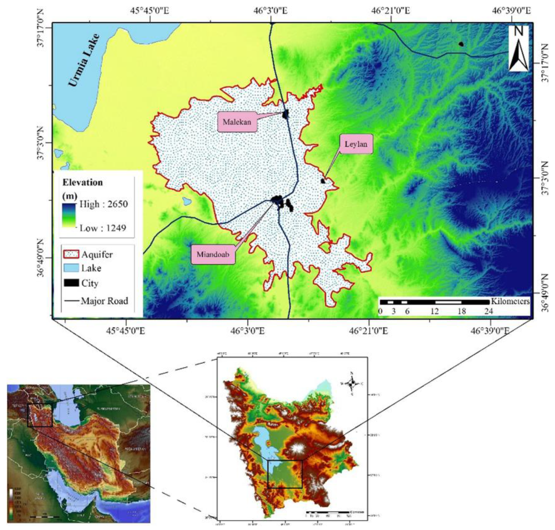
Cultivated lands of Miandoab city were for this study. Miandoab is a city in southeast Urmia province located in northwest Iran. The geographical coordinates of Miandoab are 46°2′ N and 36°58′ E at 1314 m above sea level (Figure 1). The weather in this region is variable, with relatively hot summers and cold winters. Miandoab is an essential agricultural region in West Azerbaijan province. The main crops are wheat, barley, tomato, sugar beet, corn, and apple orchards. In this region, agriculture is based on groundwater, and therefore farmers use water pumps to harvest water.

2.2. Site Designation and Experimental Treatments

Tomatoes (Monaco variety) were planted as seedlings on 15 May 2021. Two types of treatments, drip irrigation (DI) and drip irrigation with plastic mulch (PMDI), were considered. First, the potential evapotranspiration under standard conditions (ETo) was calculated by the Penman–Monteith method to calculate the water requirement. After determining the ETo, the crop coefficients (using the four-stage FAO method) were determined, and the amount of irrigation water required was calculated as follows:

$$\mathrm{IR}=\frac{{\mathrm{K}}_{\mathrm{c}}*\mathrm{ETo}}{1-\mathrm{LR}}-\mathrm{ER}$$

(1)

where IR indicates irrigation requirement (mm), Kc indicates crop coefficient, LR indicates leaching coefficient, and ER means adequate rainfall.

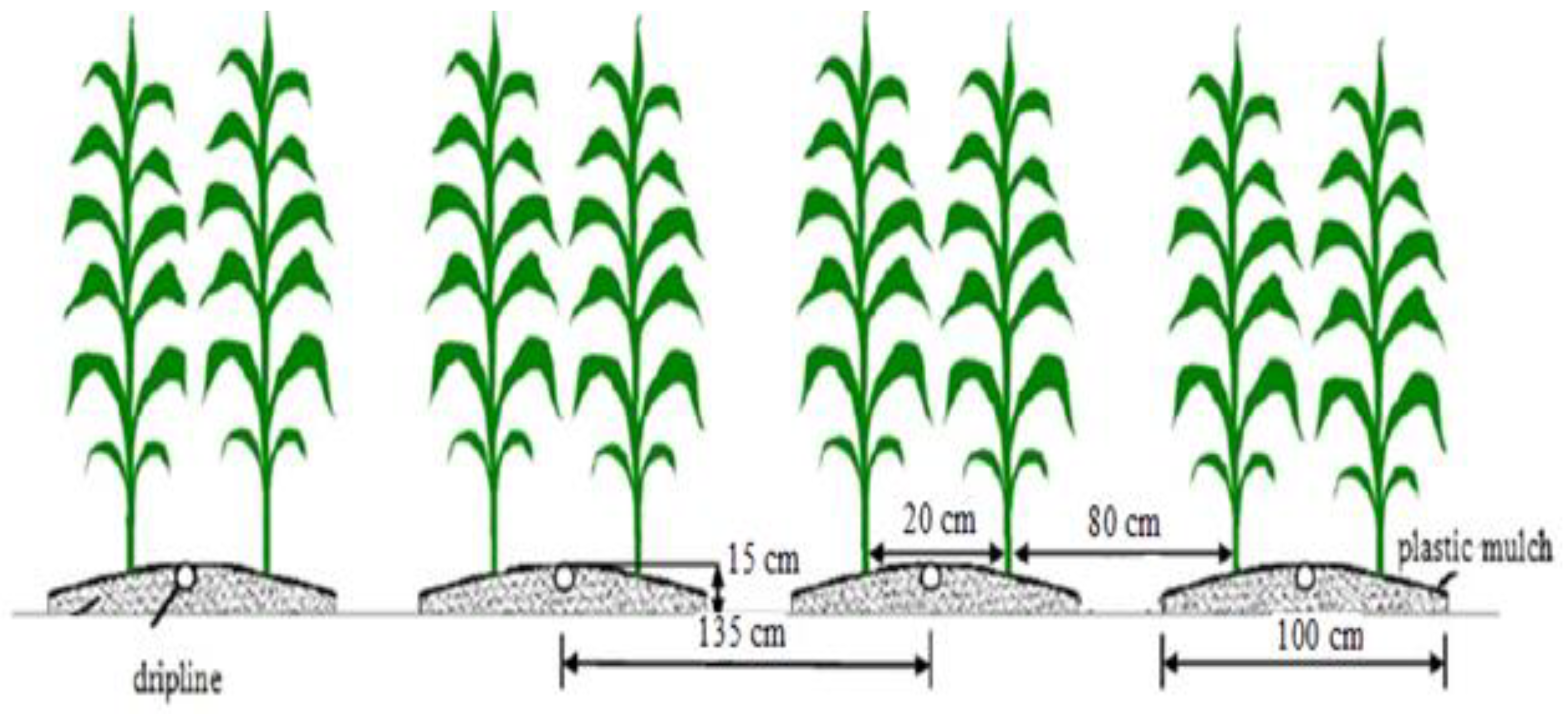
The pressure of the filtration system was 1 bar, and the inlet pressure to the irrigation tape was 0.8 bar. Water consumption was measured by a volume meter. The irrigation labyrinth drip tape with an outlet distance of 20 cm was used. Seedlings were planted on both sides of the drip tape, and cultivation intervals were considered 0.3 × 1.35. Irrigation interval in PMDI and DI treatments was considered equal to 2 and 3 days, respectively. Crop harvesting was done on August 15, August 25, and September 5, respectively.

The amount of WP of tomato crop was calculated from Equation (2):

$$\mathrm{WP}=\frac{\mathrm{Y}}{{\mathrm{W}}_{\mathrm{a}}}$$

(2)

where WP indicates water productivity, Y indicates crop yield, and W_a indicates irrigation water.

Chemical and physical analyses of soil and fertilizers used are presented in

Table 1. Chemical and physical analysis of soil at a depth of 0–30 cm.

ρb (gr/cm3)	PWP (cm3/cm3)	FC (cm3/cm3)	OC (%)	TNV (%)	θs	pH	Texture	EC (dS/m)	Silt	Sand	Clay	Depth (cm)
1.3	0.098	0.303	1.24	11.7	33	8.02	Loam	1.212	47	33	20	0–30

,

Table 2. Soil testing and crop calendar.

Area (ha)	Cultivation Pattern	Variety	Date of Planting	N (%)	P (ppm)	K (ppm)	N (Kg/ha)	P (Kg/ha)	K (Kg/ha)
1	tomato	Monaco	2021/05/05	0.1	24.2	287	50	125	150

and

Table 3. Amounts of fertilizer used.

Fertilizer	Amount	Date
Triple superphosphate	100 kg	12 May 2021
Ammonium sulfate	100 kg	12 May 2021
Potassium sulfate	175 kg	12 May 2021
Urea	50 kg	12 May 2021
Agricultural sulfur	125 kg	12 May 2021

. The data in Table 1 were used to control irrigation scheduling.

2.3. Seasons Optimization Algorithm

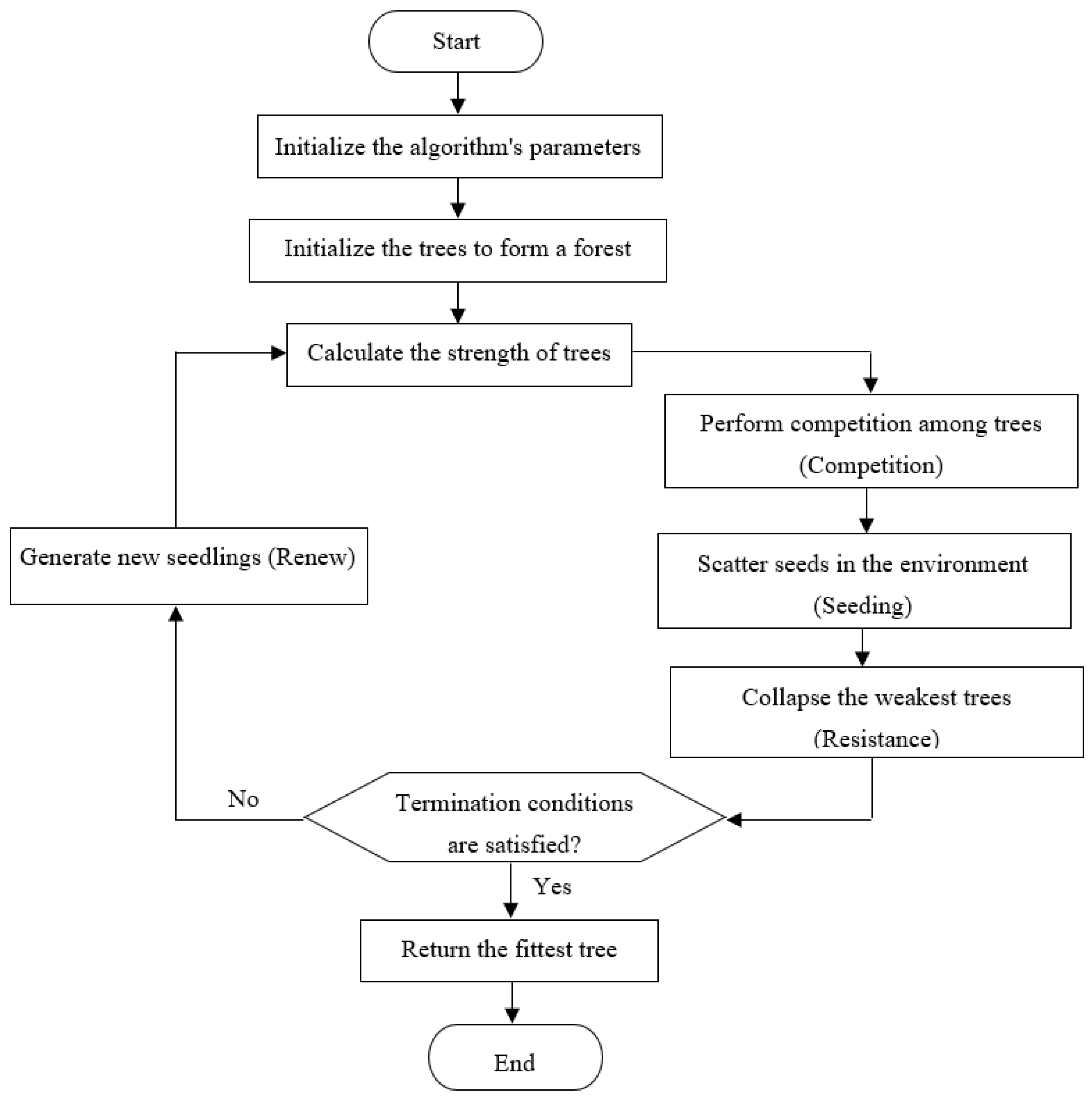
Seasons optimization (SO) is a population-based optimization meta-heuristic algorithm [33]. It models the growing process of trees in four seasons of a year. Figure 2 illustrates the flowchart of the SO algorithm. SO is an iterative algorithm in which each agent is called a tree. For solving an optimization problem, the algorithm starts its process with a population, which is called a forest. Each member of the population is called a tree, which denotes a potential solution for the given problem [33]. The algorithm updates the trees using four operators, namely renewing, competition, seeding, and resistance. The renewal phase models the impact of the spring on the growth of trees.

The competition phase modes the growth of trees in the summer. In this phase, the trees compete with their neighbor trees on shared resources, including nutrients, water, light, and other resources. To stimulate competition, the first $N_c$ most robust trees are identified.

To simulate the impact of the competition on a neighbor $T_i$, the below relationship is defined [33]:

$$\begin{array}{l}{T}_j^{y+1}=\frac{1}{{\mathsf{\Lambda }}_j+1}\times \phi (T_j^y)\\ \mathrm{where}\\ \phi (T_j^y)=T_j^y+\theta \\ {\mathsf{\Lambda }}_j={\displaystyle \sum _{k=1}^{Z_i}}{S}_k\times {\Delta }_{j,k}^{-2}\times {\lambda }_{j,k}\\ {\Delta }_{j,k}=\sqrt{{\displaystyle \sum _{z=1}^D}{(T_{jz}-T_{kz})}^2}\\ {\lambda }_{j,k}=\{\begin{array}{cc}1& \mathrm{if}(S_k\ge S_j)\\ 1-\gamma & else\end{array}\end{array}$$

(3)

where $T_j^y$ is the location of $T_j$ in the generation y. ${\mathsf{\Lambda }}_j$ is the value of competition index or crowdedness, which computes the effect of the neighbors on $T_j$. D shows the number of variables of trees. The function $\phi (.)$ calculates the growth $T_j$ in the same environment when its neighbors are ignored. $S_k$ indicates the strength/fitness of the kth neighbor tree, ${\Delta }_{j,k}$ is the distance between ${\mathsf{\Lambda }}_j$ and the kth neighbor, the variable ${\lambda }_{j,k}$ is the impact of the neighbor $T_k$ on the growth of the tree $T_j$. $\gamma \in [0,1]$ is a random asymmetry index, which shows the value to which the effect of a relatively weak neighbor is decreased.

The seeding phase is inspired by the seeding mechanism of trees in the autumn. In this phase, several trees are randomly selected and take part in the seeding phase. The resistance phase simulates the resistance of the trees against harsh winter cold. The resistance operator removes the least-strength trees from the population.

When the stopping measures are met, the algorithm updates the trees in the population by iteratively applying to renew competition, seeding, and resistance operators. Finally, the fittest tree is identified as the optimal solution [33].

2.4. Support Vector Regression (SVR)

SVR is based on support vector machine classification models [34]. SVR is used to solve nonlinear regression problems. For a brief explanation of SVR, its formulation is done. For this purpose, the dataset G is represented by Equation (4).

$$G=\left\{\begin{array}{l}(c_k,d_k)|\hspace{0.17em}k=1,2,\dots ,m\\ ,\hspace{0.17em}{c}_k\hspace{0.17em}\in \hspace{0.17em}{R}^N,\hspace{0.17em}{d}_k\in R\end{array}\right\}$$

(4)

To solve the nonlinear regression problem with SVR, first the inputs are mapped nonlinearly to the large-sized feature space f, using Equation (5). for this purpose [34]:

$$f(c_i)=\hspace{0.17em}w\phi (c_i)+b\hspace{0.17em}|\hspace{0.17em}w\in R^{M\times h},\hspace{0.17em}b\in R$$

(5)

where $\phi (c_i)$ is a function that represents the inputs from space R to space R^M×h, w indicates the weight vector, and b denotes the bias value.

b is defined as follows [34]:

$$b=\frac{1}{n}\{\sum _{0<{\gamma }_i^{-}<C}\left[d_i\hspace{0.17em}\sum _{x_j\hspace{0.17em}\in \hspace{0.17em}SV}({\gamma }_j^{+}-{\gamma }_j^{-})\hspace{0.17em}H(c_i,c_j)-\epsilon \right]+\sum _{0<{\gamma }_i^{-}<C}[d_i-\sum _{c_j\hspace{0.17em}\in \hspace{0.17em}SV}({\gamma }_j^{+}-{\gamma }_j^{-})H(c_i,c_j)+\epsilon$$

(6)

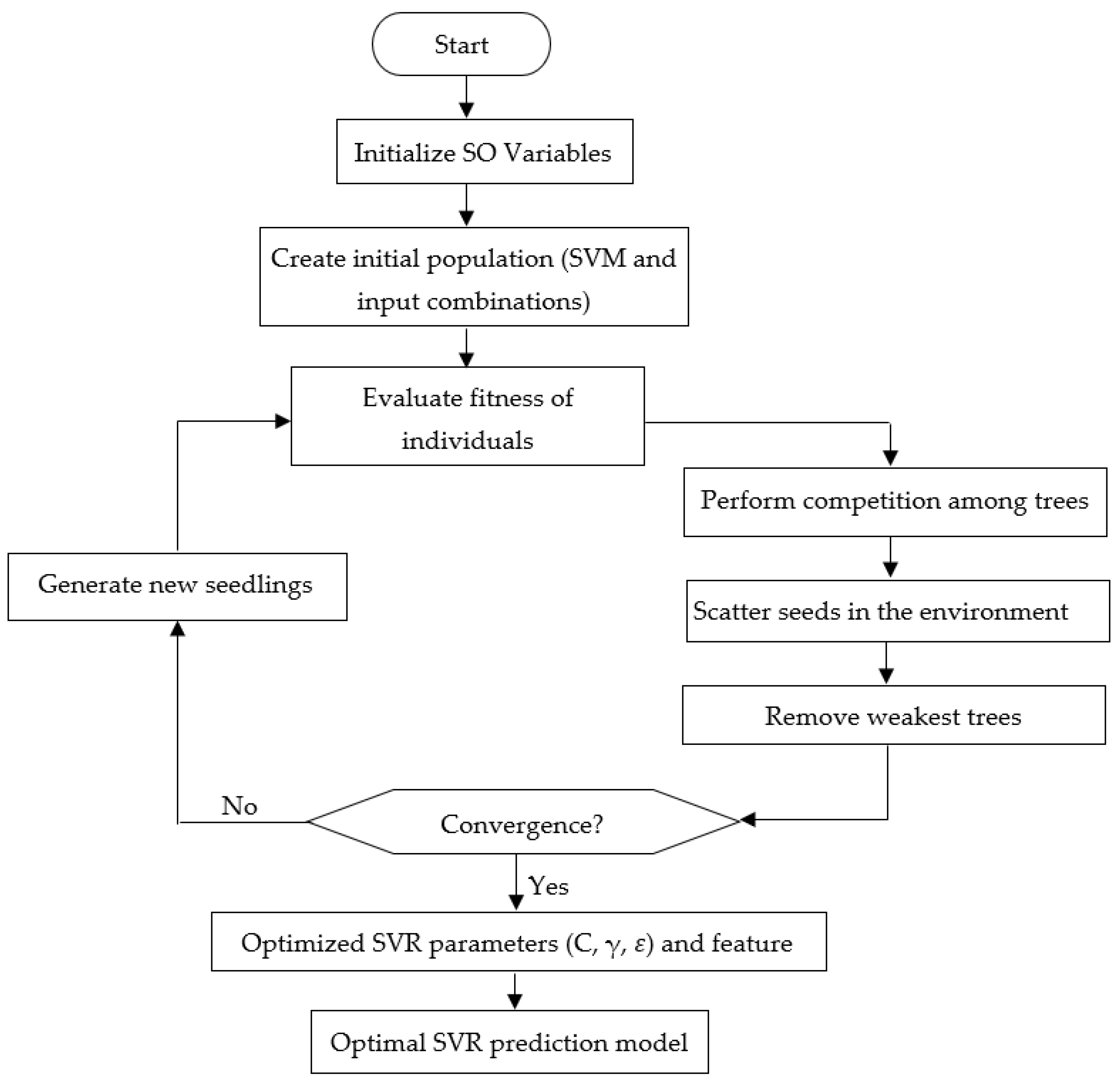
The SO algorithm has been widely compared with the most efficient recent algorithms, including evolutionary algorithms, particle swarm optimization (PSO), covariance matrix adaptation evolution strategy (CMA-ES), self-adaptive differential evolution (JDE), grey wolf optimizer (GWO), socio evolution, and learning optimization (SELO), and has given more satisfactory results [33]. Since the SO algorithm performs better in terms of solution quality and convergence rate compared to other algorithms, in this study we used it to estimate the yield and WP of tomato crops. The flowchart of the proposed SO–SVR method for selecting the SVM parameter is presented in Figure 3.

2.5. Benchmark

A wide range of climatic and irrigation–-fertilizer parameters, including water consumption during the growing season (Ir) (two levels of irrigation, drip irrigation (DI) and drip irrigation with plastic mulch (PMDI), fertilizers (N, P, K), average temperature (T_emp.avg), minimum temperature (T_emp.min), maximum temperature (T_emp.max), average relative humidity (RHavg), solar radiation (sunshine hours) (Ssh), rainfall (Pe) of each month. (http://tatweather.areeo.ac.ir/?LRef=52c6c899-7597-412d-83d7-c4cd2d05204b, 15 May to 5 September 2021), and plant variety (V), were used for experiments (

Table 4. Range of dataset parameters.

Parameter	Definition	Minimum	Maximum	Average	STDEV
Ir (DI, PMDI)	Water consumption (mm)	483.41	648.13	540.25	13.19
Temp.min	Minimum temperature (°C)	8.20	23.6	15.79	0.76
Temp.max	Maximum temperature (°C)	40.40	20.40	32.68	0.77
Temp.avg	Average temperature (°C)	15.79	32.68	26.23	1.02
RHavg	Average relative humidity (%)	19.80	61.00	32.28	1.26
Ssh	Sunshine hours (J/m2)	0.00	8.60	4.61	0.46
Pe	Rainfall (mm)	0.00	2.00	1.10	0.11
F (N, P, K)	Fertilizers used (Kg)	50	100	80	5.16
PM	Plastic mulch (−)	-	-	-	-
V	Variety (−)	-	-	-	-

). This dataset was collected on a farm with a length of 250 m, a width of 40 m, and an average slope of 0.00101 mm⁻¹ (https://earth.google.com/web/@36.96951444.45.9808815.2285.67888459a.0d.35y.0h.0t.0r?utm_source=earth7&utm_campaign=vine&hl=fa, 15 May to 5 September 2021). Of about 160 randomly selected records, 80% of the data was considered a training set and the rest a test set. Figure 4 shows a schematic of the farm used in the experiments.

2.6. Input Parameters

To evaluate the most appropriate input parameters, seven different combinations were examined. In the first step, all parameters were selected as model input, and then one of the input parameters was removed, and the proposed hybrid model was rerun (Figure 5) [1,35].

2.7. Evaluation Criteria

R², RMSE, SI, σ, and NSE indices were utilized to assess the proposed hybrid model (Table 5) [1]:

Table 5. Statistical parameters.

Criteria	No.
${\mathrm{R}}^2={\left[\frac{{\mathsf{å}}_{i=1}^{\mathrm{n}}\left(T_i-\overline{U}\right){(T}_i-\overline{U})}{{\mathsf{å}}_{i=1}^{\mathrm{n}}\sqrt{{{(T}_i-\overline{T})}^2}{\mathsf{å}}_{i=1}^{\mathrm{n}}\sqrt{{{(U}_i-\overline{U})}^2}}\right]}^2$	(7)
$\mathrm{RMSE}=\sqrt{\frac{1}{\mathrm{n}}{\displaystyle \sum _{i=1}^{\mathrm{n}}}{(T_i-U_i)}^2}$	(8)
$\mathrm{SI}=\frac{\mathrm{RMSE}}{\overline{T}}$	(9)
$\mathsf{\sigma }=\frac{{\displaystyle \sum _{i==1}^{\mathrm{n}}}\left|(U_i-T_i)\right|}{{\displaystyle \sum _{i=1}^{\mathrm{n}}}{T}_i}\times 100$	(10)
$\mathrm{NSE}=1-\frac{{\displaystyle \sum _{i=1}^{\mathrm{n}}}{(T_i-U_i)}^2}{{\displaystyle \sum _{i=1}^{\mathrm{n}}}{(T_i-\overline{U})}^2}$	(11)

Table 5. Statistical parameters.

Criteria	No.
${\mathrm{R}}^2={\left[\frac{{\mathsf{å}}_{i=1}^{\mathrm{n}}\left(T_i-\overline{U}\right){(T}_i-\overline{U})}{{\mathsf{å}}_{i=1}^{\mathrm{n}}\sqrt{{{(T}_i-\overline{T})}^2}{\mathsf{å}}_{i=1}^{\mathrm{n}}\sqrt{{{(U}_i-\overline{U})}^2}}\right]}^2$	(7)
$\mathrm{RMSE}=\sqrt{\frac{1}{\mathrm{n}}{\displaystyle \sum _{i=1}^{\mathrm{n}}}{(T_i-U_i)}^2}$	(8)
$\mathrm{SI}=\frac{\mathrm{RMSE}}{\overline{T}}$	(9)
$\mathsf{\sigma }=\frac{{\displaystyle \sum _{i==1}^{\mathrm{n}}}\left|(U_i-T_i)\right|}{{\displaystyle \sum _{i=1}^{\mathrm{n}}}{T}_i}\times 100$	(10)
$\mathrm{NSE}=1-\frac{{\displaystyle \sum _{i=1}^{\mathrm{n}}}{(T_i-U_i)}^2}{{\displaystyle \sum _{i=1}^{\mathrm{n}}}{(T_i-\overline{U})}^2}$	(11)

where, $T_i$ and $U_i$ are the estimated and observed yield and WP values, $\overline{T}$ and $\overline{U}$ are average observed and estimated yield and WP values, respectively.

3. Results

3.1. Field Monitoring

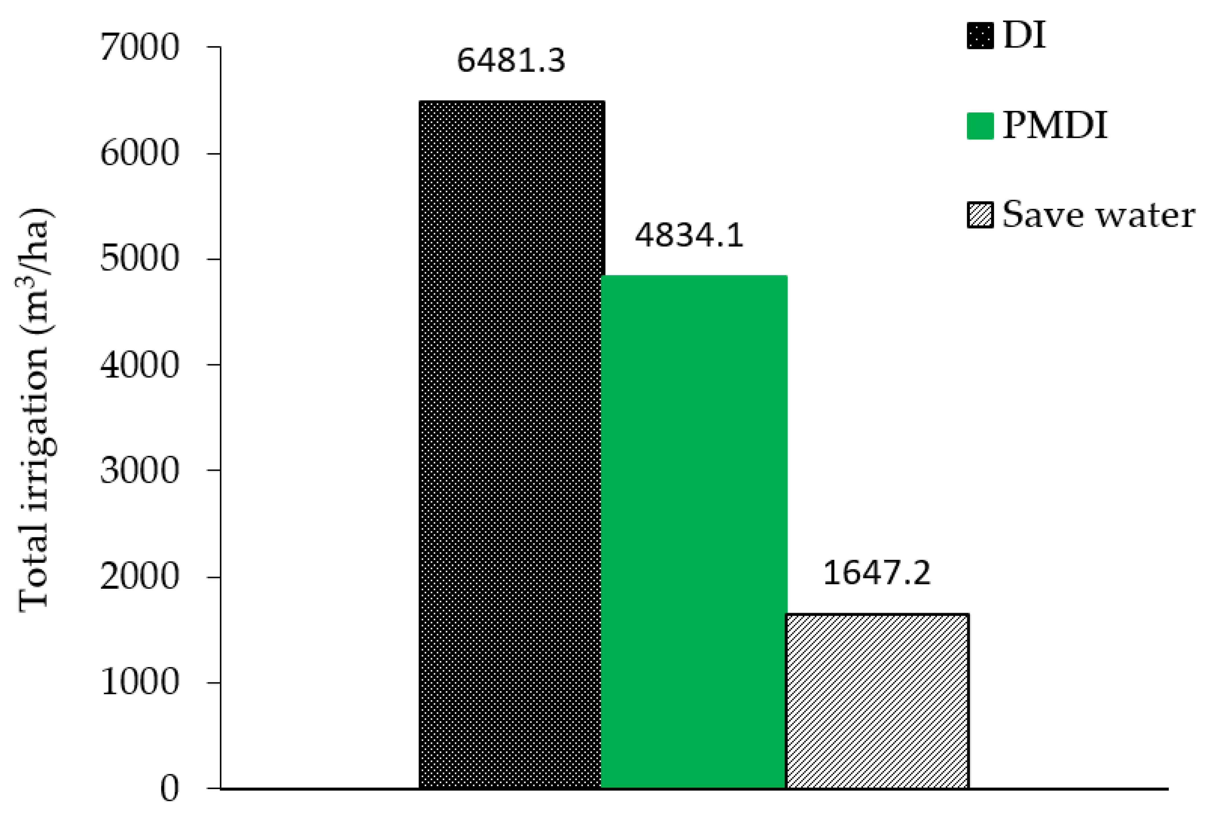
The field monitoring results are presented in

Table 6. Mean values of irrigation parameters section.

Irrigation	Qe * (L/s)		Tco ** (h)		Ig′ (mm)		AE′′ (%)
-	DI	PMDI	DI	PMDI	DI	PMDI	DI	PMDI
1	1.80	1.80	1.11	0.89	9.84	7.94	93.8	100
2	1.80	1.80	1.88	1.03	15.97	9.16	100	100
3	1.80	1.80	0.94	0.77	8.33	6.87	100	100
4	1.80	1.80	1.14	0.91	10.13	8.10	83.70	100
5	1.74	1.74	1.39	1.11	12.37	9.89	100	100
6	1.74	1.74	2.17	2.09	18.62	17.92	100	100
7	1.74	1.74	2.77	2.67	23.84	22.90	99.20	100
8	1.74	1.74	2.98	2.68	25.60	23.02	83.70	100
9	1.74	1.74	3.22	3.18	27.28	27.64	89.50	100
10	1.74	1.74	3.08	2.93	26.64	25.20	91.00	100
11	1.74	1.74	2.98	2.63	25.64	22.58	97.500	100
12	1.74	1.74	2.83	2.79	24.32	24.01	86.96	100
13	1.74	1.74	2.83	2.77	24.14	23.80	87.00	100

* Emitter discharge, ** Cut-off time, ′ Gross irrigation requirement, ′′ Water application efficiency.

. Applied water flow is the same in both irrigations treatments, but it was lower under PMDI mainly due to less water loss. Under drip irrigation systems, irrigation water applies based on the depleted water from the crop root zone. As a result, AE is usually high and it was 100% under PMDI where no water loss was recorded by evaporation from the soil surface and water depletion to under root zone. The amount of applied water in the PMDI treatment was 4834.1 m³/ha, which indicates a reduction of 25.9% of applied water in the PMDI treatment compared to DI (Figure 6). The results obtained in this study are consistent with the results of other research [36,37]. Other researchers also reported that a slight reduction in water consumption might not have a significant effect on crop yield [38,39].

The measured yield and WP in DI and PMDI treatments are presented in

Table 7. Yield and WP in research treatments.

RWC * (%)		Yield (kg/ha)		WP (kg/m3)		WP (ER **) (Kg/m3)		Improved WP (%)
DI	PMDI	DI	PMDI	DI	PMDI	DI	PMDI	DI	PMDI
-	25.90	65,000	67,500	9.96	13.96	7.87	10.28	-	30.62

* Reduction of applied water. ** Effective rainfall.

. According to the results, yield and water productivity in PMDI treatment compared to DI increased by 3.70% and 28.65%. Research has also shown that the use of plastic mulch under drip irrigation increases crop yield [40,41,42]. In general, PMDI treatment is the best treatment in cases of water shortage and increasing WP.

3.2. Modeling Results

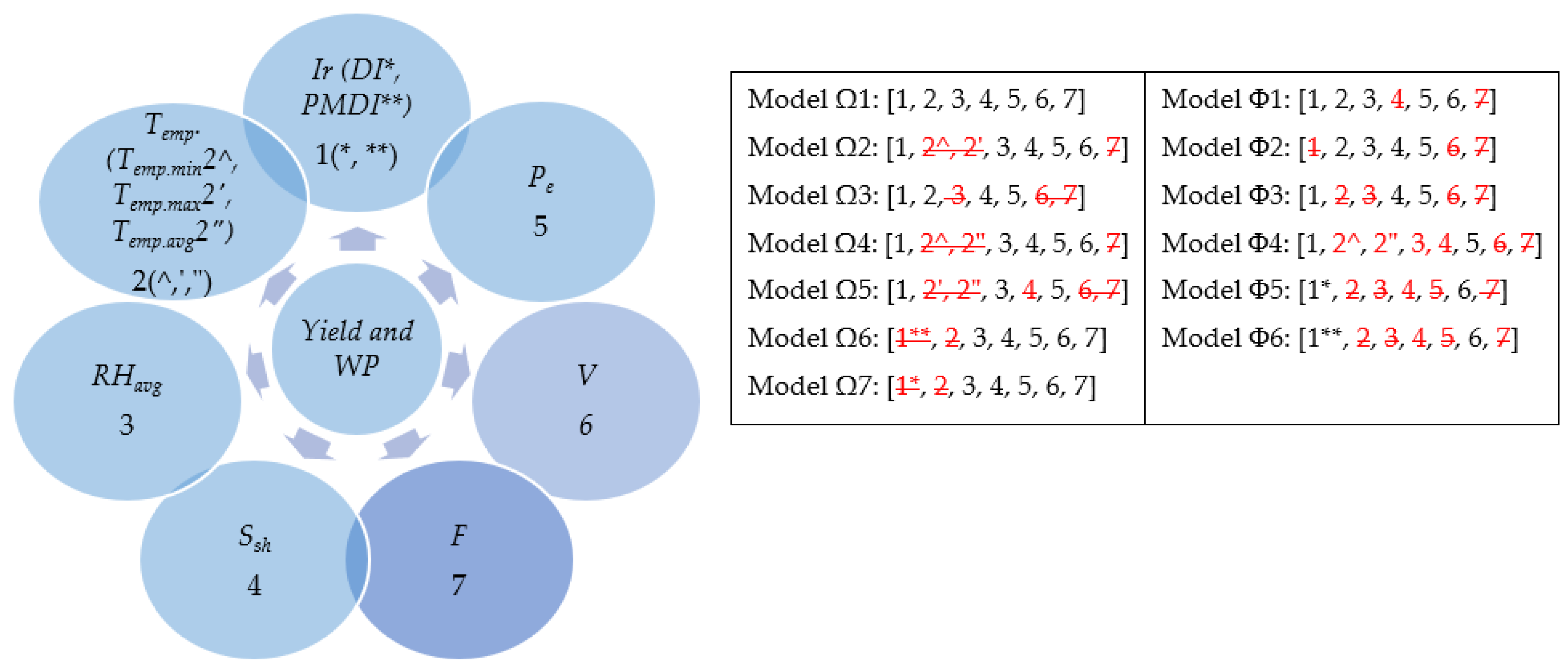
3.2.1. Impact of Input Combinations

The results obtained by the SO–SVR model using different input combinations are shown in

Table 8. Evaluation of hybrid models in yield estimation.

Model	Train					Test					SVM Parameters
	R2	RMSE	SI	σ	NSE	R2	RMSE	SI	σ	NSE	C	ε	γ
Ω1	0.980	0.009	0.012	0.888	0.960	0.961	0.010	0.015	1.125	0.914	100	0.5	1
Ω2	0.975	0.010	0.014	1.125	0.918	0.972	0.012	0.018	1.415	0.906	10	1	1
Ω3	0.890	0.012	0.016	1.142	0.846	0.851	0.020	0.033	1.650	0.705	10	0.5	1
Ω4	0.905	0.013	0.018	1.325	0.823	0.890	0.017	0.025	1.480	0.740	10	1	1
Ω5	0.880	0.015	0.026	1.589	0.725	0.868	0.019	0.031	1.620	0.710	100	0.5	1
Ω6	0.992	0.006	0.007	0.836	0.987	0.980	0.007	0.008	0.860	0.979	10	1	1
Ω7	0.994	0.005	0.006	0.794	0.989	0.982	0.006	0.007	0.614	0.982	10	1	1

and

Table 9. Evaluation of hybrid models in WP estimation.

Model	Train					Test					SVM Parameters
	R2	RMSE	SI	σ	NSE	R2	RMSE	SI	σ	NSE	C	ε	γ
Φ1	0.908	0.012	0.017	1.302	0.830	0.882	0.016	0.022	1.476	0.745	100	0.5	1
Φ2	0.882	0.014	0.023	1.574	0.732	0.870	0.018	0.029	1.615	0.725	10	1	1
Φ3	0.978	0.010	0.013	1.115	0.921	0.973	0.012	0.017	1.394	0.910	10	0.5	1
Φ4	0.981	0.009	0.011	0.875	0.961	0.962	0.010	0.013	1.158	0.916	10	1	1
Φ5	0.992	0.007	0.009	0.840	0.981	0.979	0.009	0.010	0.864	0.962	10	1	1
Φ6	0.993	0.006	0.008	0.838	0.987	0.981	0.005	0.008	0.710	0.981	10	1	1

. Psize and FE in the SO–SVR are considered 100 and 4000, respectively. The Ω7 and Φ6 models obtained the most accurate results. The irrigation–fertilizer parameters (PMDI, F) and plant variety (V) were introduced as the most influential input parameters in estimating yield and WP. Sensitivity analysis showed that after Ω7 and Φ6 models, Ω1 and Φ1 models with the input parameters of rainfall and sunshine hours also play an important role in estimating yield and WP.

According to Table 8 and Table 9, models Ω7 and Φ6 modeled the yield and WP with lower error (RMSE = 0.005–0.006) according to the irrigation–fertilizer and plant variety input parameters. Therefore, the rainfall and sunshine hours are effective parameters in determining the yield and WP, respectively. Sensitivity analysis showed that after irrigation and rainfall parameters, which affected the reproductive and leaves development of the plant, the sunshine-hours parameter (which indicates the amount of energy received by the plant) is also essential in estimating the crop yield. Sadras and Calvino showed that 90% and 76% of soybean and corn yield are affected by irrigation parameters, respectively [41]. Kaul et al. identified available water as the critical parameter in estimating crop yield [42]. Montazer et al. reported irrigation and rainfall as the most influential parameters in assessing wheat yield, which is consistent with the results of the present study [43].

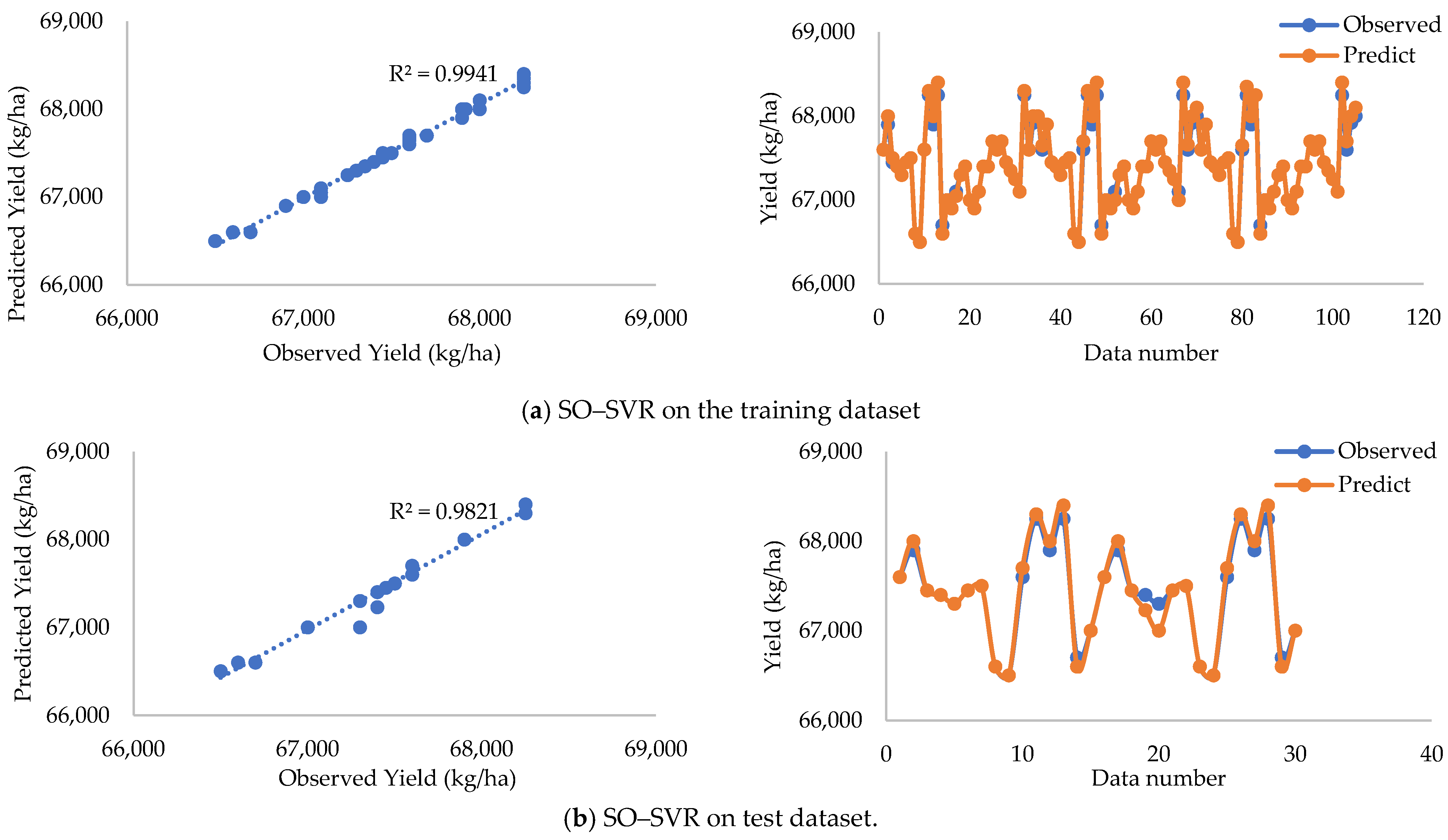
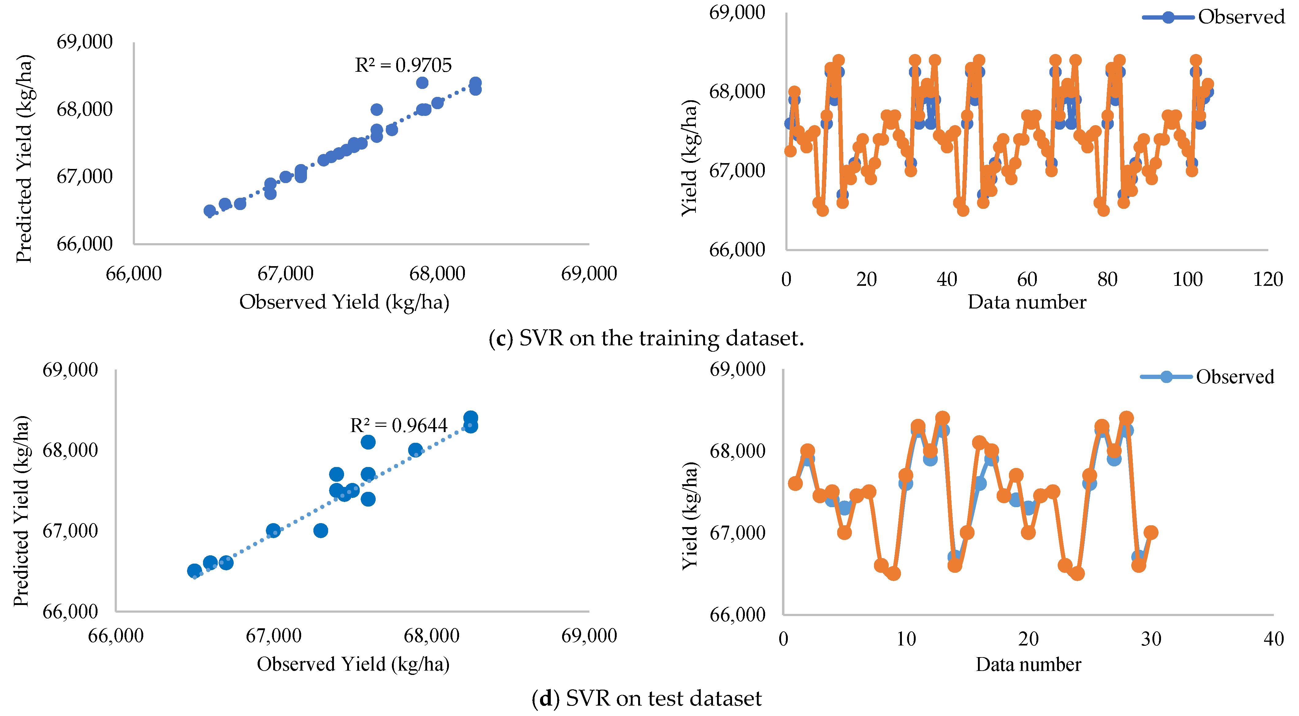
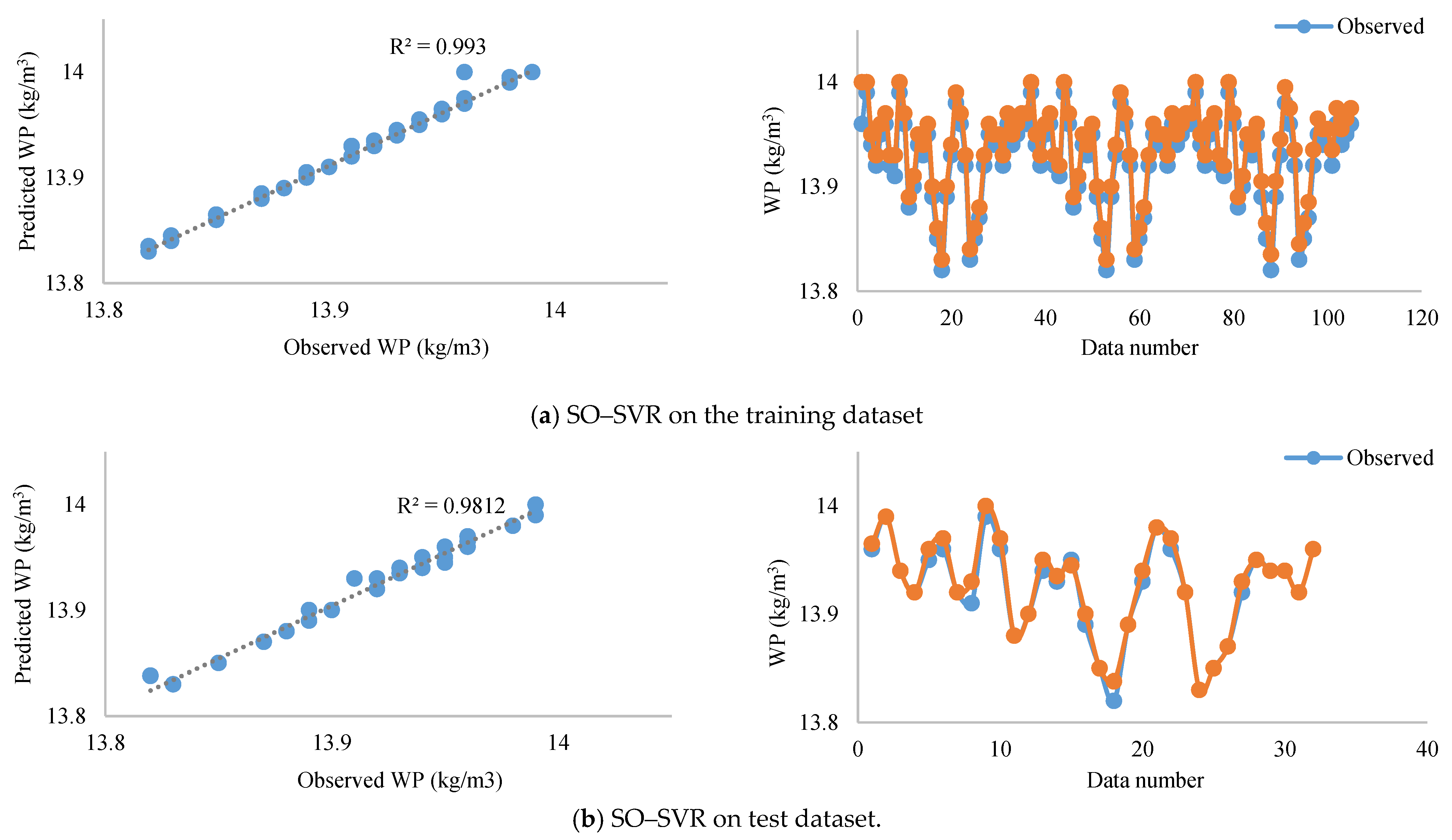
According to Figure 7 and Figure 8, it is clear that the yield and WP using the SO–SVR hybrid method are estimated with high accuracy and are in appropriate agreement with the observed values.

The results indicate that for both yield and WP traits, the proposed hybrid model yields slightly higher WP and crop yield values compared to the observed value, which is due to the relatively high accuracy of the hybrid model in this study. Based on the results, calculating the average temperature (Temp._avg), minimum temperature (Temp._min), maximum temperature (Temp._max), and average relative humidity (RH_avg), parameters have little effect on reducing the RMSE error, but appending rainfall (P_e) and solar radiation (S_sh) parameters reduce the RMSE. The results of this study are consistent with the results of previous research. Hosseini et al. obtained the accuracy of predicting wheat yield in Qorveh province in northwestern Iran using an artificial neural network of 0.99 [44].

The optimal results obtained using the hybrid SO–SVR model in the test and training stages for models Ω7 and Φ6 are given in

Table 10. Evaluation of SO–SVR method in the training stage.

Method	R2	RMSE	SI	σ	NSE
SO–SVR	0.994	0.005	0.006	0.794	0.989
SVR	0.970	0.015	0.019	1.412	0.920

and

Table 11. Evaluation of SO–SVR method in the test stage.

Method	R2	RMSE	SI	σ	NSE
SO–SVR	0.982	0.006	0.007	0.812	0.982
SVR	0.964	0.018	0.022	1.161	0.912

.

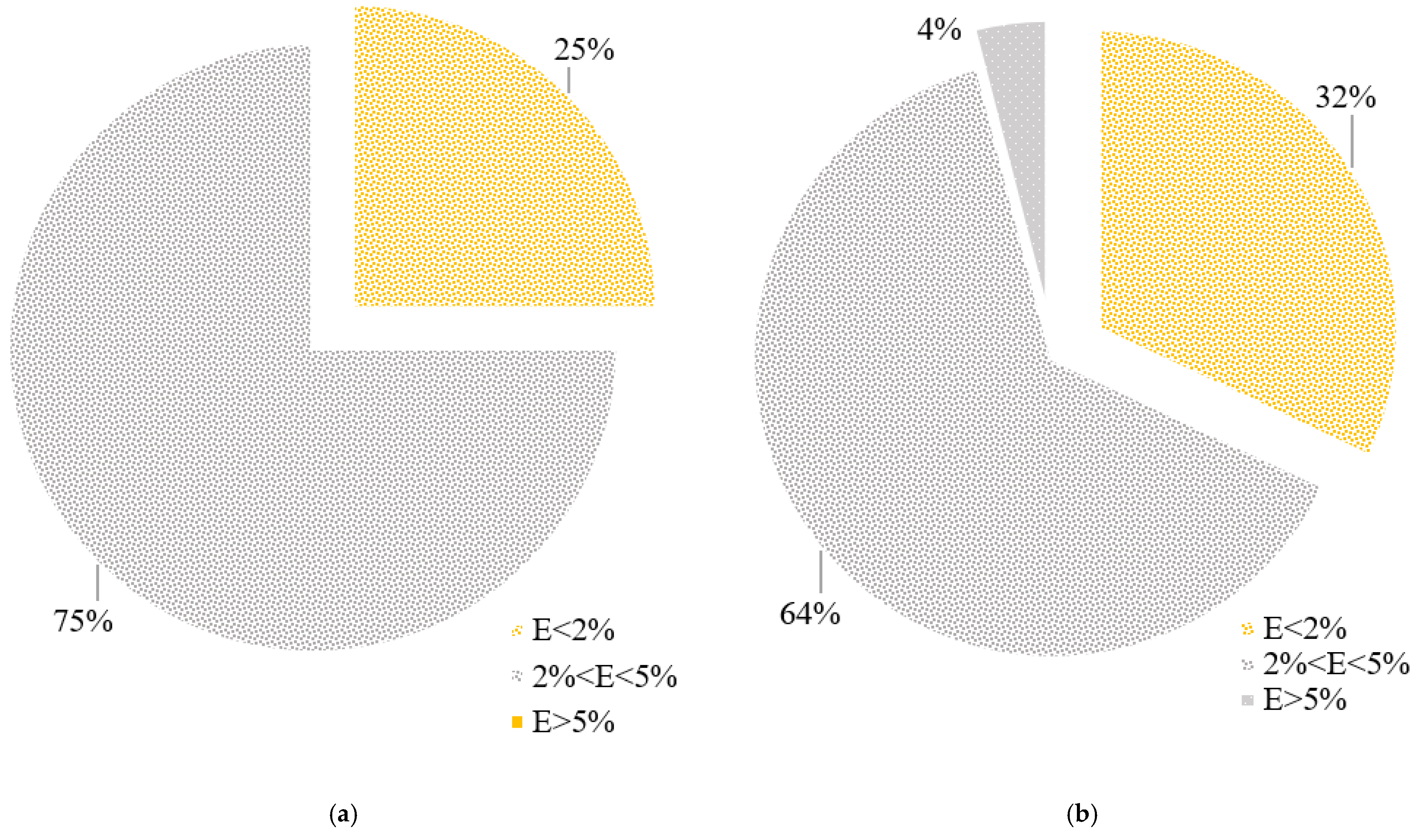
Figure 9 shows the error distribution diagrams of SO–SVR and SVR on the test stage. The results show that about 75% of the yield values estimated utilizing the SO–SVR have an error of less than 2%, while in the SVR, 64% of the yield values calculated have an error of less than 2%.

3.2.2. Comparison with Other Methods

Due to the limited use of soft computing methods in WP estimation and yield, the SO–SVR method with Ω7 and Φ6 models are compared with previous studies by Sharifi [45] and Prasad et al. [46]. In

Table 12. Comparison of SO–SVR model with other methods.

Model	R2	RMSE	SI	σ	NSE
GPR	0.840	0.055	-	-	0.835
RF	0.690	0.045	-	-	0.687
SVR	0.964	0.018	0.022	1.161	0.912
SO–SVR	0.982	0.006	0.007	0.614	0.982

, the SO–SVR hybrid model is compared with the results of other studies. The SO–SVR method with R² of 0.982 had better performance than the Gaussian process regression algorithm (GPR) and random forest (RF) with R² of 0.84 and 0.69, respectively. The superiority of the SO–SVR hybrid method compared to other methods is the excellent performance of the SO algorithm in finding the optimal parameters of the SVR method.

4. Conclusions

This paper investigates the influence of drip irrigation and plastic mulch on tomato yield and introduces the SO–SVR hybrid method to estimate WP and yield. The average improvement of WP and the reduction of applied water in PMDI treatment compared to DI were 34.10% and 39.20%, respectively. The results showed that the observed and estimated values were in good agreement. To determine the most appropriate effective parameters in estimating WP and yield, seven models with different input combinations were selected, respectively. The Ω7 and Φ6 models with input combinations including irrigation–fertilizer parameters (PMDI, F) and plant variety (V) were introduced as the superior models. In addition, the results indicate that the SO–SVR hybrid model has a good capability in estimating yield and WP with R² = 0.982, RMSE = 0.006, SI = 0.007, σ = 0.614, and NSE = 0.982, respectively. The SO algorithm is a high-speed convergence algorithm and performed better than its peer algorithms in optimizing SVR parameters and thus estimating the yield and WP of tomato crop. However, the SO–SVR model needs to be parameterized, and the performance of the SO–SVR is a bit far from ideal. Therefore, it is recommended that for future research the SO algorithm be combined with adaptive neuro-fuzzy inference models and artificial neural networks to improve the defects and provide generalizable results.

References

- Emami, S.; Parsa, J.; Emami, H.; Abbaspour, A. An ISaDE Algorithm Combined with Support Vector Regression for Estimating Discharge Coefficient of W-Planform Weirs. Water Supply 2021, 21, 3459–3476. [Google Scholar] [CrossRef]
- Safa, M.; Samarasinghe, S. Determination and Modelling of Energy Consumption in Wheat Production Using Neural networks: “A Case Study in Canterbury Province, New Zealand”. Energy 2011, 36, 5140–5147. [Google Scholar] [CrossRef] [Green Version]
- Trigui, M.; Gabsi, K.; Amri, I.E.; Noureddine, A. International Journal of Food Properties Modular Feed Forward Networks to Predict Sugar Diffusivity from Date Pulp Part I. Model Validation. Int. J. Food Prop. 2011, 14, 37–41. [Google Scholar] [CrossRef]
- Fortin, J.G.; Anctil, F.; Parent, L.É.; Bolinder, M.A. Site-Specific Early Season Potato Yield Forecast by Neural Network in Eastern Canada. Precis. Agric. 2011, 12, 905–923. [Google Scholar] [CrossRef]
- Basso, B.; Cammarano, D.; Carfagna, E. Review of Crop Yield Forecasting Methods and Early Warning Systems. First Meet. Sci. Advis. Comm. Glob. Strateg. Improv. Agric. Rural Stat. 2013, 241, 1–56. [Google Scholar]
- Gonzalez-Sanchez, A.; Frausto-Solis, J.; Ojeda-Bustamante, W. Attribute Selection Impact on Linear and Nonlinear Regression Models for Crop Yield Prediction. Sci. World J. 2014, 2014, 509429. [Google Scholar] [CrossRef] [PubMed]
- Gupta, D.K.; Kumar, P.; Mishra, V.N.; Prasad, R.; Dikshit, P.K.S.; Dwivedi, S.B.; Ohri, A.; Singh, R.S.; Srivastava, V. Bistatic Measurements for the Estimation of Rice Crop Variables Using Artificial Neural Network. Adv. Space Res. 2015, 55, 1613–1623. [Google Scholar] [CrossRef]
- Bocca, F.F.; Rodrigues, L.H.A. The Effect of Tuning, Feature Engineering, and Feature Selection in Data Mining Applied to Rainfed Sugarcane Yield Modelling. Comput. Electron. Agric. 2016, 128, 67–76. [Google Scholar] [CrossRef]
- Ravichandran, G.; Koteeshwari, R.S. Agricultural Crop Predictor and Advisor Using ANN for Smartphones. In Proceedings of the 2016 International Conference on Emerging Trends in Engineering, Technology and Science (ICETETS), Pudukkottai, India, 24–26 February 2016; pp. 2–7. [Google Scholar] [CrossRef]
- Gandhi, N.; Petkar, O.; Armstrong, L.J. Rice Crop Yield Prediction Using Artificial Neural Networks. In Proceedings of the 2016 IEEE Technological Innovations in ICT for Agriculture and Rural Development (TIAR), Chennai, India, 15–16 July 2016; pp. 105–110. [Google Scholar] [CrossRef]
- Merdun, H.; Çinar, Ö.; Meral, R.; Apan, M. Comparison of Artificial Neural Network and Regression Pedotransfer Functions for Prediction of Soil Water Retention and Saturated Hydraulic Conductivity. Soil Tillage Res. 2006, 90, 108–116. [Google Scholar] [CrossRef]
- Mubiru, J. Predicting Total Solar Irradiation Values Using Artificial Neural Networks. Renew. Energy 2008, 33, 2329–2332. [Google Scholar] [CrossRef]
- Piri, J.; Amin, S.; Moghaddamnia, A.; Keshavarz, A.; Han, D.; Remesan, R. Daily Pan Evaporation Modeling in a Hot and Dry Climate. J. Hydrol. Eng. 2009, 14, 803–811. [Google Scholar] [CrossRef]
- Xing, L.; Li, L.; Gong, J.; Ren, C.; Liu, J.; Chen, H. Daily Soil Temperatures Predictions for Various Climates in United States Using Data-Driven Model. Energy 2018, 160, 430–440. [Google Scholar] [CrossRef]
- Maya Gopal, P.S.; Bhargavi, R. A Novel Approach for Efficient Crop Yield Prediction. Comput. Electron. Agric. 2019, 165, 104968. [Google Scholar] [CrossRef]
- Yari, R.; Darzi-Naftchali, A.; Dehghanisanij, H.; Qi, Z. Effect of Meteorological Data Quality Control and Data Adjustment on the Reference Evapotranspiration: A Case Study in Jafariye, Iran. Theor. Appl. Climatol. 2020, 141, 331–342. [Google Scholar] [CrossRef]
- Liu, S.; Wang, X.; Liu, M.; Zhu, J. Towards Better Analysis of Machine Learning Models: A Visual Analytics Perspective. Vis. Inform. 2017, 1, 48–56. [Google Scholar] [CrossRef]
- Haghverdi, A.; Washington-Allen, R.A.; Leib, B.G. Prediction of Cotton Lint Yield from Phenology of Crop Indices Using Artificial Neural Networks. Comput. Electron. Agric. 2018, 152, 186–197. [Google Scholar] [CrossRef]
- Hund, L.; Schroeder, B.; Rumsey, K.; Huerta, G. Distinguishing between Model- and Data-Driven Inferences for High Reliability Statistical Predictions. Reliab. Eng. Syst. Saf. 2018, 180, 201–210. [Google Scholar] [CrossRef]
- Akbar, A.; Kuanar, A.; Patnaik, J.; Mishra, A.; Nayak, S. Application of Artificial Neural Network Modeling for Optimization and Prediction of Essential Oil Yield in Turmeric (Curcuma Longa L.). Comput. Electron. Agric. 2018, 148, 160–178. [Google Scholar] [CrossRef]
- Matsumura, K.; Gaitan, C.F.; Sugimoto, K.; Cannon, A.J.; Hsieh, W.W. Maize Yield Forecasting by Linear Regression and Artificial Neural Networks in Jilin, China. J. Agric. Sci. 2015, 153, 399–410. [Google Scholar] [CrossRef]
- Dehghanisanij, H.; Naseri, A.; Anyoji, H.; Eneji, A.E. Effects of Deficit Irrigation and Fertilizer Use on Vegetative Growth of Drip Irrigated Cherry Trees. J. Plant Nutr. 2007, 30, 411–425. [Google Scholar] [CrossRef]
- Ji, B.; Sun, Y.; Yang, S.; Wan, J. Artificial Neural Network Model for Rice Yield Prediction in Mountainous Regions. J. Agric. Sci. 2007, 145, 249–261. [Google Scholar] [CrossRef]
- Higashide, T. Prediction of Tomato Yield on the Basis of Solar Radiation before Anthesis under Warm Greenhouse Conditions. HortScience 2009, 44, 1874–1878. [Google Scholar] [CrossRef] [Green Version]
- Alvarez, R. Predicting Average Regional Yield and Production of Wheat in the Argentine Pampas by an Artificial Neural Network Approach. Eur. J. Agron. 2009, 30, 70–77. [Google Scholar] [CrossRef]
- Norouzi, M.; Ayoubi, S.; Jalalian, A.; Khademi, H.; Dehghani, A.A. Predicting Rainfed Wheat Quality and Quantity by Artificial Neural Network Using Terrain and Soil Characteristics. Acta Agric. Scand. Sect. B Soil Plant Sci. 2010, 60, 341–352. [Google Scholar] [CrossRef]
- Anitha, P.; Chakravarthy, T. Agricultural Crop Yield Prediction Using Artificial Neural Network with Feed Forward Algorithm. Int. J. Comput. Sci. Eng. 2018, 6, 178–181. [Google Scholar] [CrossRef]
- Lin, D.; Wei, R.; Xu, L. An Integrated Yield Prediction Model for Greenhouse Tomato. Agronomy 2019, 9, 873. [Google Scholar] [CrossRef] [Green Version]
- Abrougui, K.; Gabsi, K.; Mercatoris, B.; Khemis, C.; Amami, R.; Chehaibi, S. Prediction of Organic Potato Yield Using Tillage Systems and Soil Properties by Artificial Neural Network (ANN) and Multiple Linear Regressions (MLR). Soil Tillage Res. 2019, 190, 202–208. [Google Scholar] [CrossRef]
- Dehghanisanij, H.; Kouhi, N. Interactive Effects of Nitrogen and Drip Irrigation Rates on Root Development of Corn (Zea Mays L.) and Residual Soil Moisture. Gesunde Pflanz. 2020, 72, 335–349. [Google Scholar] [CrossRef]
- Jeevan Nagendra Kumar, Y.; Spandana, V.; Vaishnavi, V.S.; Neha, K.; Devi, V.G.R.R. Supervised Machine Learning Approach for Crop Yield Prediction in Agriculture Sector. In Proceedings of the 2020 5th International Conference on Communication and Electronics Systems (ICCES), Coimbatore, India, 10–12 June 2020; pp. 736–741. [Google Scholar] [CrossRef]
- Rodrigues, M.Â.; Torres, L.d.N.D.; Damo, L.; Raimundo, S.; Sartor, L.; Cassol, L.C.; Arrobas, M. Nitrogen Use Efficiency and Crop Yield in Four Successive Crops Following Application of Biochar and Zeolites. J. Soil Sci. Plant Nutr. 2021, 21, 1053–1065. [Google Scholar] [CrossRef]
- Emami, H. Seasons Optimization Algorithm. Eng. Comput. 2020. [Google Scholar] [CrossRef]
- Drucker, H.; Surges, C.J.C.; Kaufman, L.; Smola, A.; Vapnik, V. Support Vector Regression Machines. Adv. Neural Inf. Process. Syst. 1997, 9, 155–161. [Google Scholar]
- Hamzeh, A.; Parsaie, A.; Ememgholizadeh, S. Prediction of Discharge Coefficient of Triangular Labyrinth Weirs Using Adaptive Neuro Fuzzy Inference System. Alex. Eng. J. 2017, 57, 1773–1782. [Google Scholar] [CrossRef]
- Akhavan, S.; Moosavi, S.F.; Mostafazadehfard, B.; Ghadamifiroozabadi, A. Investigation of Yield and Water Use Efficiency of Potato with Tape and Furrow Irrigation. J. Water Soil Sci. 2007, 11, 15–27. [Google Scholar]
- Yuan, B.Z.; Nishiyama, S.; Kang, Y. Effects of Different Irrigation Regimes on the Growth and Yield of Drip-Irrigated Potato. Agric. Water Manag. 2003, 63, 153–167. [Google Scholar] [CrossRef]
- Wang, F.X.; Feng, S.Y.; Hou, X.Y.; Kang, S.Z.; Han, J.J. Potato Growth with and without Plastic Mulch in Two Typical Regions of Northern China. Field Crop. Res. 2009, 110, 123–129. [Google Scholar] [CrossRef]
- Qin, S.; Zhang, J.; Dai, H.; Wang, D.; Li, D. Effect of Ridge-Furrow and Plastic-Mulching Planting Patterns on Yield Formation and Water Movement of Potato in a Semi-Arid Area. Agric. Water Manag. 2014, 31, 87–94. [Google Scholar] [CrossRef]
- Hou, X.Y.; Wang, F.X.; Han, J.J.; Kang, S.Z.; Feng, S.Y. Duration of Plastic Mulch for Potato Growth under Drip Irrigation in an Arid Region of Northwest China. Agric. For. Meteorol. 2010, 150, 115–121. [Google Scholar] [CrossRef]
- Sadras, V.O.; Calviño, P.A. Quantification of Grain Yield Response to Soil Depth in Soybean, Maize, Sunflower, and Wheat. Agron. J. 2001, 93, 577–583. [Google Scholar] [CrossRef]
- Kaul, M.; Hill, R.L.; Walthall, C. Artificial Neural Networks for Corn and Soybean Yield Prediction. Agric. Syst. 2005, 85, 1–18. [Google Scholar] [CrossRef]
- Montazer, A.; Azadeghan, B.; Shahraki, M. Assessing the Efficiency of Artificial Neural Network Models to Predict Wheat Yield and Water Productivity Based on Climatic Data and Seasonal Water-Nitrogen Variables. Iran. Water Res. J. 2010, 3, 17–29. [Google Scholar]
- Hosseini, S.M.T.; Siosemardeh, A.; Fathi, P.; Siosemardeh, M. Application of Artificial Neural Networks and Multivariate Regression in Estimating Dryland Wheat Yield in Qorveh Region of Kurdistan Province. Agric. Res. 2007, 7, 41–54. [Google Scholar]
- Sharifi, A. Yield Prediction with Machine Learning Algorithms and Satellite Images. J. Sci. Food Agric. 2021, 101, 891–896. [Google Scholar] [CrossRef] [PubMed]
- Prasad, N.R.; Patel, N.R.; Danodia, A. Crop Yield Prediction in Cotton for Regional Level Using Random Forest Approach. Spat. Inf. Res. 2021, 29, 195–206. [Google Scholar] [CrossRef]
Figure 1.
Geographical location map.
Figure 2.
Flowchart of the season optimization (SO) algorithm.
Figure 3.
Flowchart of the SO– support vector regression (SVR).
Figure 4.
Schematic of the experimental setup.
Figure 5.
Combinations of input parameters to estimated yield and WP. * Drip irrigation, ** Drip irrigation with plastic mulch, ^ Minimum temperature, ’ Maximum temperature, " Average temperature.
Figure 6.
Comparison of total applied water in research treatments.
Figure 7.
(a–d) Comparison of predicted yield with observed results in the training and test stages.
Figure 8.
(a,b) Comparison of predicted WP with observed results in the test and training stages.
Figure 9.
Error distribution of (a) SO–SVR and (b) SVR on test stage.