Effect of Subsurface Mediterranean Water Eddies on Sound Propagation Using ROMS Output and the Bellhop Model

Abstract

Ocean processes can locally modify the upper ocean density structure, leading to an attenuation or a deflection of sound signals. Among these phenomena, eddies cause significant changes in acoustic properties of the ocean; this suggests a possible characterization of eddies via acoustics. Here, we investigate the propagation of sound signals in the Northeastern Atlantic Ocean in the presence of eddies of Mediterranean Water (Meddies). Relying on a high-resolution simulation of the Atlantic Ocean in which Meddies were identified and using the Bellhop acoustic model, we investigated the differences in sound propagation in the presence and absence of Meddies. Meddies create sound channels in which the signals travel with large acoustic energy. The transmission loss decreases to 80 or 90 dB; more signals reach the synthetic receivers. Outside of these channels, the sound signals are deflected from their normal paths. Using receivers at different locations, the acoustic impact of different Meddies, or of the same Meddy at different stages of its life, are characterized in terms of angular distributions of times of arrivals and of energy at reception. Determining the influence of Meddies on acoustic wave characteristics at reception is the first step to inverting the acoustic signals received and retrieving the Meddy hydrological characteristics.

1. Introduction

Ocean acoustics is the science of sound processes in the ocean and is concerned in particular with sound generation, propagation, attenuation and deflection [1,2]. This science is essential to understand marine mammal communication, for seismic studies, oceanographic applications, acoustic tomography, sonar detection and underwater engineering. Sound propagation in the ocean strongly depends on variations of temperature, salinity, pressure and on the presence of currents [3]. In particular, surface and internal waves, eddies (oceanic vortices), inflow/outflow of water masses with different thermohaline characteristics, fronts, seabed sedimentation, etc. affect the propagation of sound waves in the sea [4]. The focus of our study is the influence of subsurface oceanic eddies on sound propagation. The attention given to subsurface eddies, which are numerous and play an important role in ocean dynamics but are little known in terms of their acoustic impact, is a novelty of this work.

Mesoscale (radius = 10–100 km) and submesoscale (radius = 1–10 km) eddies are ubiquitous in the ocean [5,6]. They are long-lived horizontally recirculating fluid motions, strongly constrained by the rotation of the Earth and by ocean stratification. Eddies are found at different depths in the water column [7]. They have a deep imprint in the physical, chemical and biological structure of the ocean. In particular, they strongly contribute to the meridional transport of momentum, heat and salt across the oceans [8,9]. Cyclonic and anticyclonic eddies have different thermohaline structures and rotations [10,11], which affect sound propagation differently, though their presence is always associated with a noticeable gradient of sound speed.

Previous studies have addressed the question of the impact of oceanic eddies on sound propagation, mostly for surface intensified eddies. Henrick et al. (1980) [12] introduced an acoustic model that related sound speed variations to the eddy radii and rotation rates. Bong-Chae et al. (2012) [13] investigated eddies in the East/Japan Sea near the Korean Peninsula. They discovered how a warm eddy affects sound propagation: the low-frequency sound propagation from the eddy center to the eddy edge is more affected by the eddy in comparison with the sound propagation from the eddy edge to the eddy center. In another study, Li Jia et al. (2012) [14] found that an eddy with a warm core can make the acoustic convergence zone recede and increase its width, while a cold eddy has an opposite effect. Using the parabolic equation (PE), Lawrence (1983) [14] calculated the transmission loss as a function of depth and distance for an acoustic signal crossing the Tasman warm eddy. By examining CTD (Conductivity-Temperature-Depth) temperature and salinity data, Qingyu (2006) [15] studied how an eddy affected the structure of the sound velocity and concluded that it affected the surface velocity gradient and the structure of the deep sound channel. Baer (1980) [16], showed that the location of the eddy relative to the source causes changes in transmission loss of as much as 20 dB.

Nearly all the above studies were associated with sound propagation through a surface eddy at a given instant; no investigation was carried out to determine how deep eddies at different stages of their life affect sound propagation. Subsurface vortices play a key dynamical role in the oceans but determining their 3D structure and geographical distribution is a difficult task because of their small size. Pointwise measurements may thus miss such eddies. Therefore, using integral measurements of changes in acoustic properties of the ocean is more likely to identify subsurface eddies by quantifying such changes on long vertical sections of the ocean. Our project has a two-fold objective: first, quantify the changes in acoustic propagation due to subsurface eddies (the work reported in this paper) and then invert these measurements to recover the structure and distribution of subsurface eddies in the ocean. In this paper we address the first objective.

A well-known and dynamically active variety of subsurface eddies are Meddies (Mediterranean Water eddies). Mediterranean Water flows into the Atlantic Ocean through the Straits of Gibraltar and generates an outflow along the south and west Iberian coast, and a plume in the northeastern Atlantic Ocean. Meddies are formed from the instability of the Mediterranean outflow [17,18]. They may also originate from the interaction of the Mediterranean Water plume with seamounts, currents or surface-intensified eddies [19]. These Meddies are intensified around 1000 m depth. Their horizontal extent varies from 30 to 100 km, while their vertical extent varies from 500 to 1000 m. They have a positive temperature and salinity anomaly (up to 4 °C and 1 psu) with respect to the surrounding ocean. They are often long-lived (from 1.5- to 4-year lifetimes). They mostly form near the Iberian Peninsula, and then drift southwestwards [19,20]. Up to 15–20 Meddies can form each year. Therefore, Meddies are frequent in the Northeastern Atlantic Ocean. In particular, we concentrate here on anticyclonic Meddies (the cyclonic Meddies, generally referred to as deep cyclones of Mediterranean Water, will be studied in another article). Here we will quantify how Meddies affect the spatial propagation of sound signals locally, and how they modify the acoustic amplitude and the time of arrival of sound signals at receivers lying at different depths downstream of the Meddy.

The present study is a first step to quantify these parameters (acoustic amplitude, time of arrival) with respect to the Meddy structure and position with respect to the source and receiver. The long-term goal is to invert the parameters and to recover the radial-vertical structure of the Meddy via a neural network (this will be the subject of a future study). In particular, we will then address the complementarity of the acoustic and of surface dynamical information (sea surface height anomalies related to the eddy).

The key result of this study is that the acoustic impact of Meddies is measurable and can be clearly attributed to these eddies; sound receivers placed at different depths and distances from the acoustic source can identify distinct Meddies or the same Meddy at different stages of its life.

Here, we use the results from a realistic, three-dimensional ocean model (ROMS), applied to the Northeastern Atlantic Ocean; this model simulates the formation, propagation and decay of Meddies. The hydrodynamical model output allows us to calculate their acoustic impact. In particular, we identify and investigate Meddies at different stages of their lifetime. Section 2 presents the material and methods (oceanic and acoustic models); Section 3 provides the results of the acoustic model, analyses them and discusses these results. Section 4 gives the main conclusions and perspectives of the study.

2. Materials and Methods

2.1. Ocean Model

2.1.1. Model Characteristics and Forcing

Sound propagation within Meddies is studied here using the temperature and salinity fields provided by a high-resolution numerical simulation of the Northeastern Atlantic Ocean [19]. The simulation is run in the 4.5° W to 20° W and 32° N to 41° N area (depicted in Figure 1) and is based on the Regional Ocean Modeling System (ROMS). ROMS is a 3-D free surface, sigma-coordinate, split-explicit primitive equation model for the ocean, based on the Boussinesq and hydrostatic approximations, with ocean thermodynamics and an equation of state for seawater [21]. The resolution of the horizontal grid is about 3 km, and the vertical grid is composed of 32 unequally spaced levels, stretched in order to have higher resolutions near the surface. The model resolution is suitable to represent mesoscale eddies with radii about 30–50 km and vertical extents ranging from 400 to 1000 m. The time integration is performed every 300 s and the outputs are given by three-day averages [19]. The model was run for 24 years (starting from the year 2000, model time) with atmospheric forcing provided by a climatological database [22]. Given the climatological forcing, the model time is not in phase with actual dates. Nevertheless, in our study we will keep the standard date format for simplicity.

2.1.2. Eddy Tracking

The Meddies’ trajectories were obtained by applying an eddy tracking software to the numerical simulation described in Section 2.1.1 [19,23]. We restricted our analyses to four Meddies with lifetimes exceeding 1 year; their trajectories are presented in Figure 1 and they are automatically numbered by the tracking software.

Meddy 33 (red trajectory in Figure 1) was chosen as a reference for investigating the impact of Meddies on sound signals. During its life cycle, it exhibited common features of Meddies found in the real ocean and sampled via in-situ measurements [24]. Meddy 33 tended to grow in size and rotation rate from its early stages to its mid-term; it then progressively decayed until its latest detection [25]. We will use it as a case study and show the generality of our results in comparison with the other Meddies. Additional Meddies will be examined at their mid-term evolution (see Section 3.2).

Meddy 33 lifetime was about 3 years; its radius was around 35 km. It had a swirl velocity around 30 cm/s and extended vertically over 1000 m [25]. This Meddy was first detected by the tracking software on 1 January 2004 in the model simulation (at the position 11° W, 37° N). It exhibited a southwestward trajectory and reached the edge of the modelled domain on 9 June 2006 (model time).

2.2. Acoustic Model

2.2.1. Bellhop Model

Since Meddies evolve near and below the oceanic thermocline, we use an acoustic ray model which is suitable to simulate sound propagation in the deep ocean: the Bellhop acoustic model [26]. The Bellhop program package is part of the Toolbox AcTUP—Acoustic Toolbox User-interface & Post-processor to Matlab. This toolbox provides the user with a working environment, automating the creation of code-specific initialization files and guesses, as well as selection guidelines for code specific parameters [27]. An analysis dataset is used to establish the environment for acoustic modeling and simulation. Bellhop is based on the theory of normal modes, and it uses the boundary element method to obtain the transmission loss. The program calculates the transmission loss (TL) due to discrete modes, specifically those which propagate only via total reflection and refraction.

Reflection and refraction are two important phenomena in the field of sound signal propagation. Reflection occurs at the surface and the bottom, and refraction occurs inside the water mass. When the sound signals propagate, reflection occurs only in the surface and the bottom, but refraction occurs more frequently for all signals, whether for those that reach the surface or the bottom or for those that do not reach the surface or the bottom. After passing through different layers and successive refractions, the signals reach the surface or the bottom at different angles from the angle of emission and are finally reflected from there. Refractions also occur when signals pass through different layers. However, since the focus of the present paper is on the reflections of sound signals, more emphasis is laid on the reflection than the refraction.

The present study investigates how sound signals propagate considering their angles of emission and reception using the results from the Bellhop model. Each signal is emitted at an angle between −35° and 35° (see also Section 3.1.1). The time of arrival of sound signals is related to their transmission loss and to the number of their reflections at the oceanic surface and bottom.

The way the signals propagate in the environment also affects their time of arrival. The sound signals evolve differently according to their angles of emission. In the −10° to 10° range of angles, they mostly evolve along straight lines without undergoing any reflections and only with small refractions. However, for angles larger than 10° and −10°, the signals are reflected from the oceanic surface and bottom. The larger the number of the signals that are reflected, the later they arrive at the receivers. Additionally, as the number of reflections of sound signals from the surface and the bottom increases, the sound signals lose more energy, and transmission loss also increases, so that sometimes some signals cannot reach the receiver.

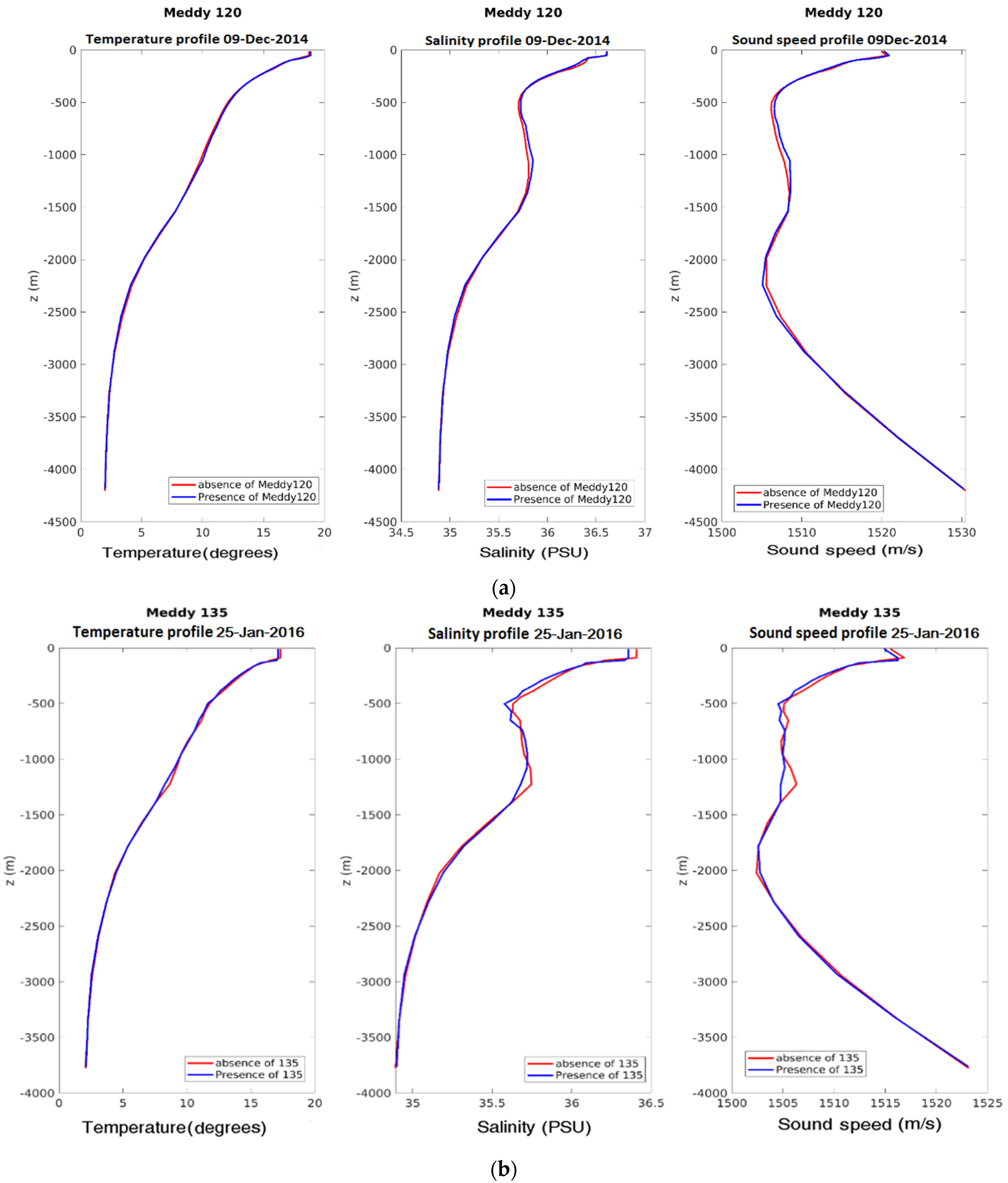
2.2.2. Sound Speed Feature

The sound speed in the ocean is a function of three variables: temperature, salinity, and pressure (depth). The sound speed increases with the increase of any of the three parameters following the empirical formula presented below [26,28,29,30].

$$C=1448.96+\left(4.591T\right)-\left(5.304\ast {10}^{-2}{T}^2\right)+\left(2.374\ast {10}^{-4}{T}^3\right)+\cdots$$

(1)

where C is the sound speed in m/s, Z is the depth in m, T represents the temperature in degrees Celsius and S stands for the salinity in PSU.

Figure 2 shows a vertical section of the sound speed, along the 36.5° N parallel, in our study area (the Northeastern Atlantic Ocean) on 7 August 2004. In this figure, sound speed anomalies are related to depth, temperature and salinity variations due to the presence of currents, eddies and filaments of Mediterranean Water (like the one located at 1000 m depth and 13° W, the Meddy 33 discussed in Section 2.1.2).

A Hovmoller diagram shows the time evolution of the vertical profile of sound speed at Meddy 33’s center (from 31 January 2004 until July 2006; Figure 3). This figure indicates that the sound speed undergoes different changes with time at depths between the surface and 100 m, between 800 to 1600 m or between 1600 and 3200 m. In surface and near-surface layers, temperature and salinity are affected by the atmospheric forcing; in particular, as the Meddy drifts southwestward, the surface temperature increases and so does the sound speed. The second noticeable change is that Meddy 33 decays away from its generation site near the Iberian Peninsula. As salt and heat diffuse from the Meddy core to its environment, the sound speed anomaly decreases in the Meddy core. More generally, heat and salt diffusion from all Meddies feed the Mediterranean Water “tongue” (or plume) which extends from the Strait of Gibraltar to the mid-Atlantic Ridge. Finally, as the Meddy moves away from the eastern boundary of this geographical domain, it flows above colder and fresher waters such as the Labrador Sea Water (LSW) and the North Atlantic Deep Water (NADW). The acoustic signature of these water masses appears via the decrease in sound speed at depths between 1600 and 3200 m. Below 3500 m depth, the Antarctic Bottom Water (AABW) is relatively uniform in this area.

2.2.3. Methodology Used to Calculate the Acoustic Impact of Meddies

In this paper, we compare the acoustic signals reaching different locations using synthetic receivers placed at different depths and horizontal distances from the acoustic source (see e.g., Section 3.1.2 or Figure A1, Figure A2 and Figure A3 for more details). This is firstly investigated for a section crossing the Meddy core (with a spatially varying sound speed, dependent on the hydrological properties of this Meddy) and secondly for a “reference” section outside the Meddy, created by extending uniformly horizontally the acoustic properties of a point outside the Meddy periphery. This latter section reflects the hydrological and acoustic properties of the ocean, locally, at rest (in the absence of the Meddy).

3. Results

Firstly, we investigate the impact of Meddy 33 on acoustic propagation during its lifetime, focusing on its early stage (6 February 2004), mid-term structure (28 January 2005) and at its latest detection stage (9 June 2006). Then, we will compare the results for Meddy 33 with those of the other long-lived Meddies in the numerical simulation (their trajectories are depicted in Figure 1).

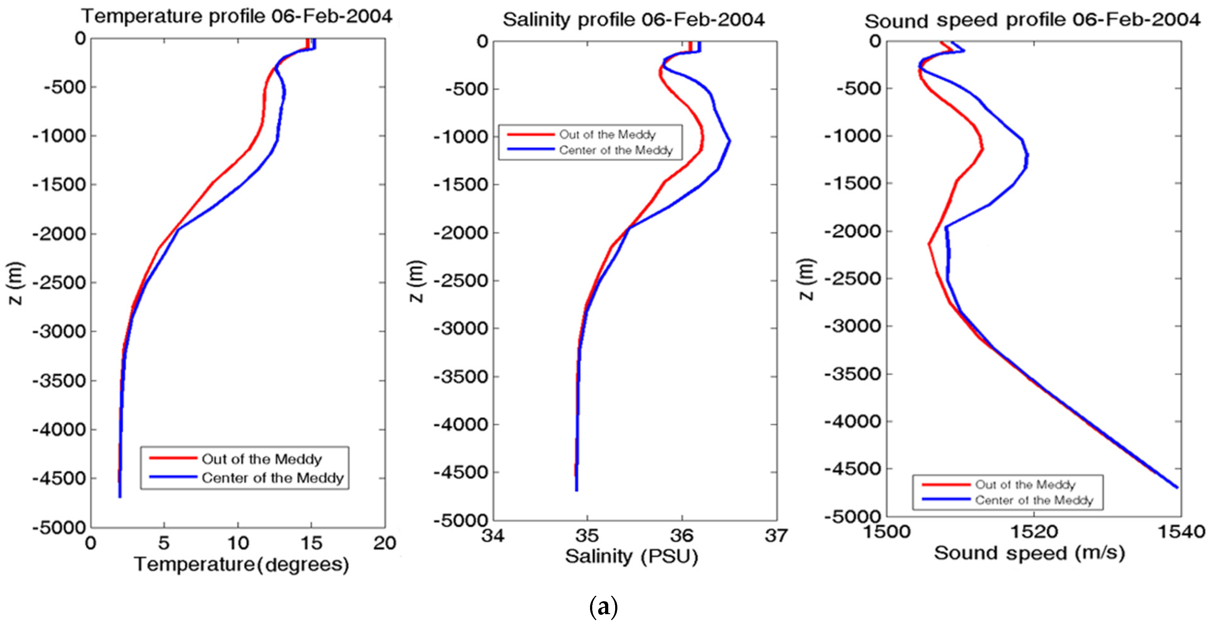
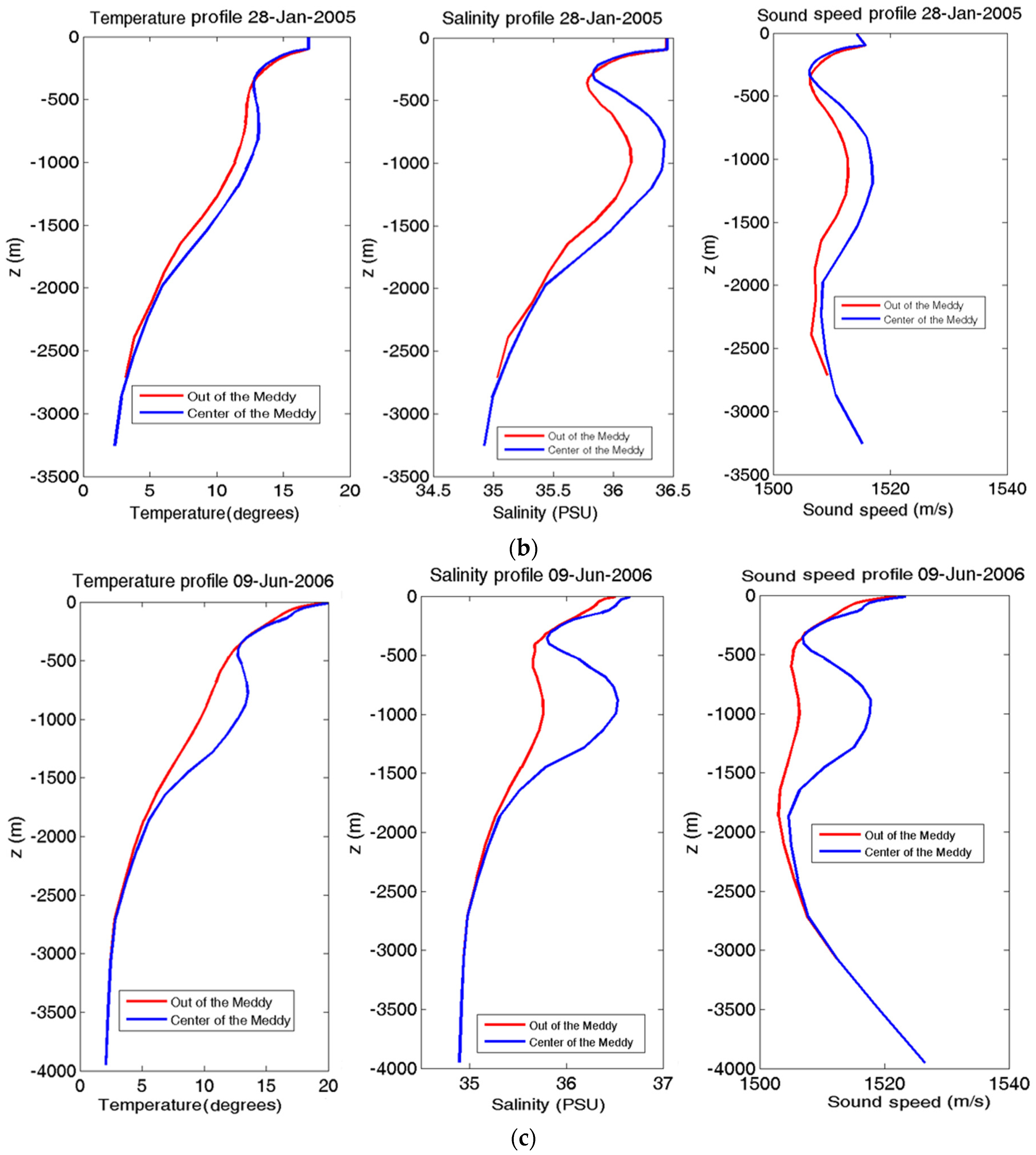
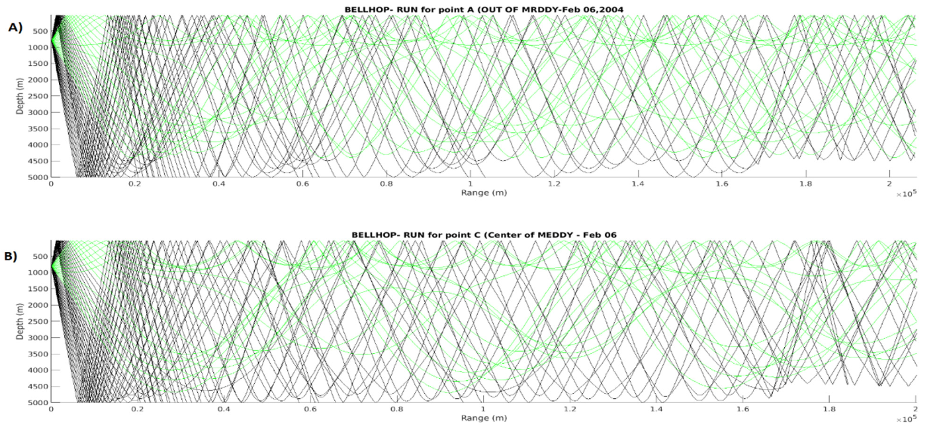
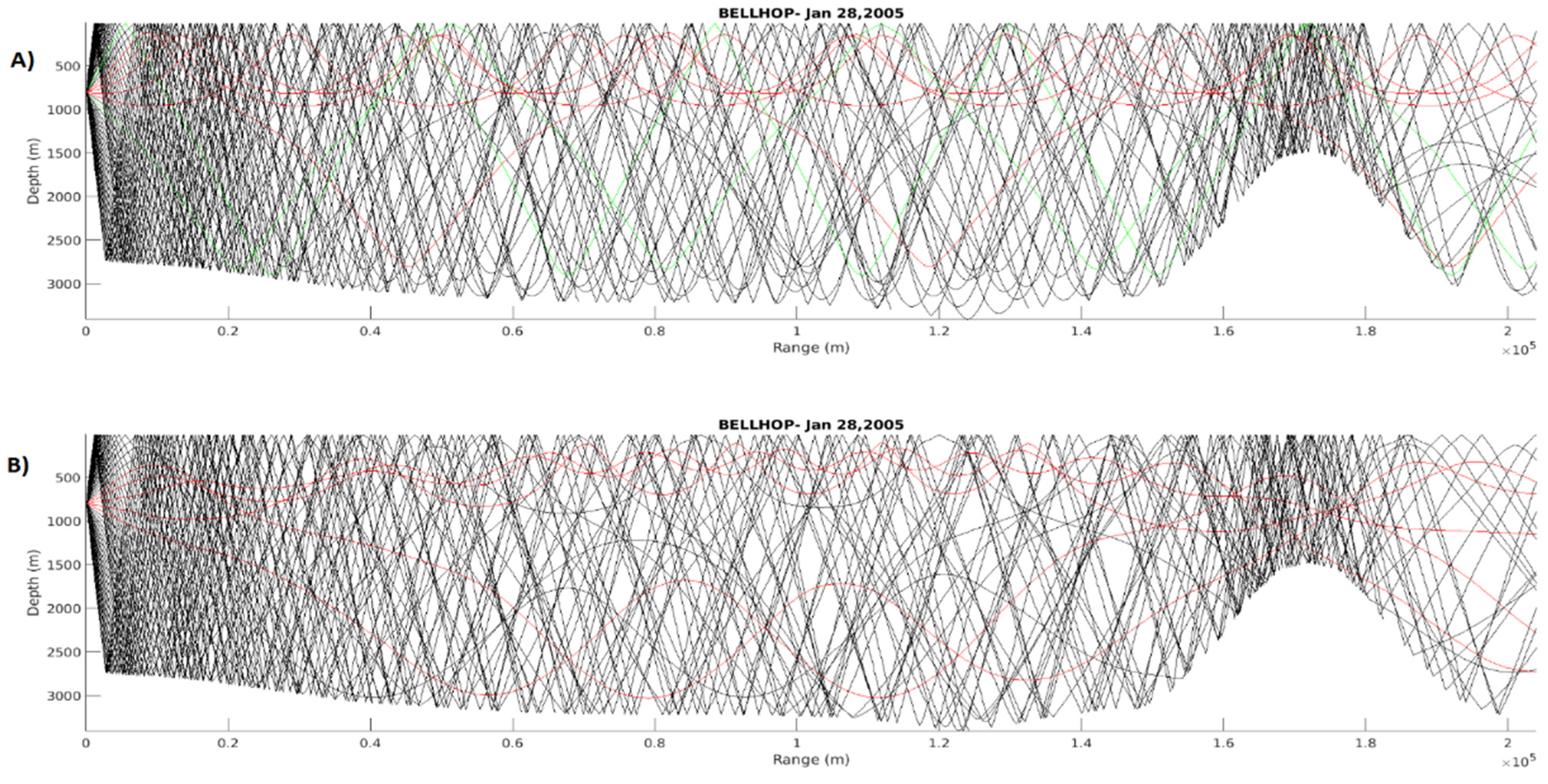
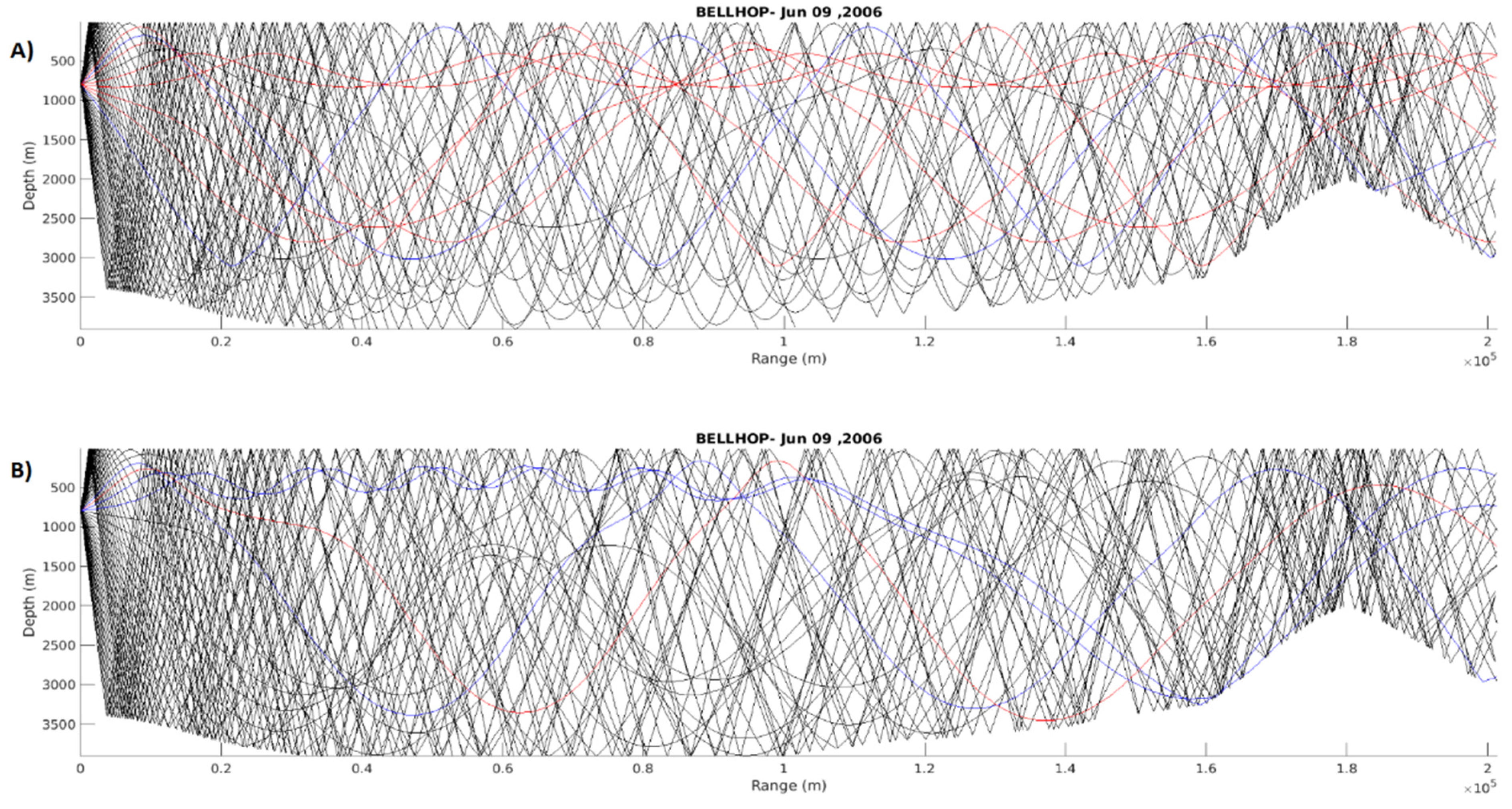
3.1. The Reference Case (Meddy 33)

In Figure 4, the horizontal structure of Meddy 33 at different dates is shown: the physical quantity represented is the Ertel Potential Vorticity (EPV) anomaly. In a primitive equation model, EPV is expressed by (2):

$$EPV=\left(\frac{\partial v}{\partial x}-\frac{\partial u}{\partial y}+f\right)\left(\frac{\partial \rho }{\partial z}\right)-\frac{\partial v}{\partial z}\frac{\partial \rho }{\partial x}+\frac{\partial u}{\partial z}\frac{\partial \rho }{\partial y}$$

(2)

where f is the Coriolis parameter, $\rho$ is the seawater density, and (u, v) are the two components of horizontal velocity. The EPV Anomaly (EPVA) is the difference between the local Ertel potential vorticity and that of the ocean at rest:

$$EPVA=EPV-f\frac{\partial \rho }{\partial z}$$

(3)

Clearly, Meddy 33 is close to an elliptical shape in EPVA at these three stages of its evolution. It is surrounded by a few filaments or a ring of an opposite-signed EPVA which isolates it from the surrounding ocean.

Below, we firstly show the hydrological properties of the ocean at two locations: at the Meddy center (called point B) and at a point outside of the Meddy (called point A), which far away to avoid its influence and to be representative of the Meddy environment. On 6 February 2004, point A is 128 km north of point B; on 28 January 2005, A is 59 km north of B, and on 9 June 2006, A is 47 km north of B. The position of these points are shown in Figure 4b. The profiles of sound speed, salinity and temperature for points A and B are presented in Figure 5 at three stages in the life of Meddy 33. For the three dates, the maximal salinity, temperature and sound speed lie in the Meddy core, as expected. On 6 February 2004, the sound speed profile reached a maximum at depths between 300 and 2000 m. In the Meddy, the sound speed was around 1517 to 1520 m/s, while values around 1509 to 1512 m/s were found out of it. The presence of the Meddy created sound channels between the surface and nearly 1000 m depth, and between approximately 1500 and 3500 m depth. On 9 June 2006 (Meddy 33’s latest stage) the sound speed at the sea surface was 1525 m/s, higher than at any other depth, most likely due to the onset of summertime near-surface stratification. This lowered the probability of sound signals to reach the ocean surface because sound signals propagate towards areas with lower sound speed. The only signals which can reach the surface were those emitted at angles larger than ±20°.

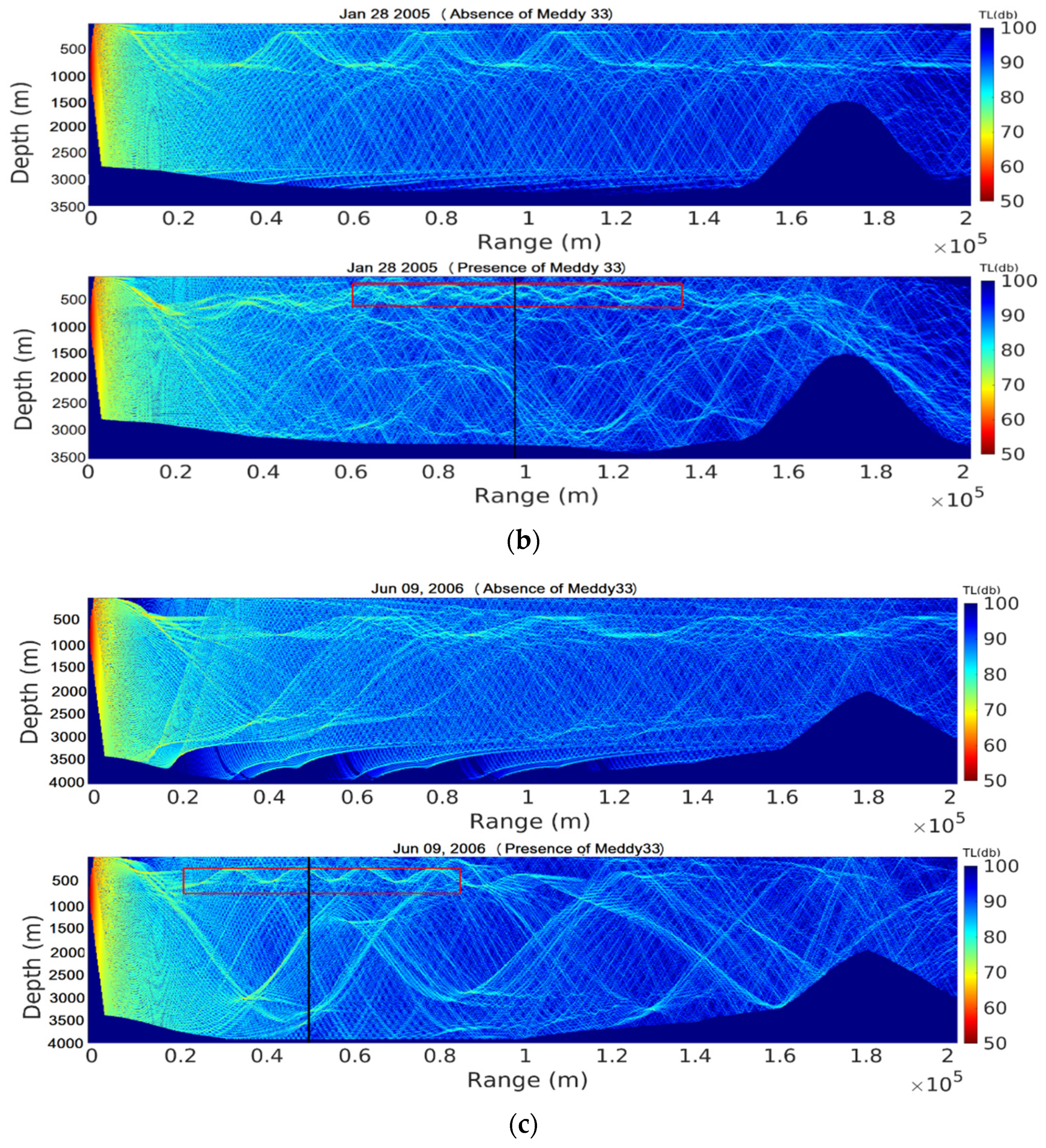
3.1.1. Sound Propagation and Transmission Loss (Vertical Sections)

Now, we study the sound propagation and transmission loss in vertical reference sections and sections across Meddy centers. The reference sections were created as follows: the vertical profile of salinity, temperature and sound speed at each point B was extended uniformly horizontally. This contrasts with the Meddy sections, where strong horizontal in homogeneities of T, S and C occur. These Meddy sections were extracted from the ROMS model output.

The depth of the simulated sound source (Ds) was chosen as 800 m near a local maximum of sound speed. The sound velocity at this depth is about 1510 m/s. A sound source at this depth allows sound signals with small or large angles of emission to propagate upwards or downwards. In our study, sound signals are emitted with angles between −35° to 35°, but only the signals emitted between −24° and 24° reach the receivers. Indeed, the signals emitted at angles larger than ±24° are reflected at the bottom or surface at narrow angles. These numerous reflections and refractions dampen the signals, preventing them from reaching the receivers.

The source frequency is 200 Hz. The acoustic range considered for all cases is 201 km. The position of the source and successive positions of the receivers are shown in Figure A1, Figure A2 and Figure A3 in the Appendix A with respect to the position of the Meddy. Meddy 33 was located in areas with different bathymetries for three dates: 5000 m depth on 6 February 2004, 3500 m on 28 January 2005 and 4000 m on 9 June 2006. Figure A4, Figure A5 and Figure A6 in the Appendix A show the propagation of individual sound signals. Here, Figure 6 shows the transmission losses for all dates.

On 6 February 2004, in the control section, no acoustic signal propagated directly from the source to the receiver without reflection. An acoustic channel was observed between the surface and the 800 m depth with multiple reflections. In the section with Meddy 33, the sound signals were deflected to the surface and could not reach the bottom. The depth of the sound channel increased in comparison with the control section; the sound signals intensified, and the transmission loss decreased to 80 dB. In particular, the transmission loss decreased near the surface (upper 500 m), between 1000 to 1500 m depth, near the bottom (from 4000 m down to the bottom) and also at long range (between 195 to 200 km), (Figure 6a).

On 28 January 2005, in the control section, acoustic signals were concentrated in a channel extending from the sea surface to 1000 m depth. In the section with Meddy 33, the sound signals separated into two channels. Part of the signals were focused near the Meddy and formed a sound channel down to 500 m depth; the other signals travelled in a deeper channel below 1000 m depth. Between the 2 sound channels, the transmission loss increased (almost from 85 to 90 dB). After crossing the Meddy, the sound signals in the surface sound channel were deflected downwards and merged with the deep sound channel. The acoustic signals were intense (travel with large acoustic energy) in the sound channel. The Meddy favored their propagation along the range; thus, the transmission loss decreased (Figure 6b).

On 9 June 2006, the Meddy induced again 2 sound channels (between the surface and 800 m depth and between 1500 and 3000 m). The signal in the shallower sound channel was deflected downwards after crossing the Meddy and was reflected upwards from the ocean bottom. This modified the signal transmission loss in the area (Figure 6c).

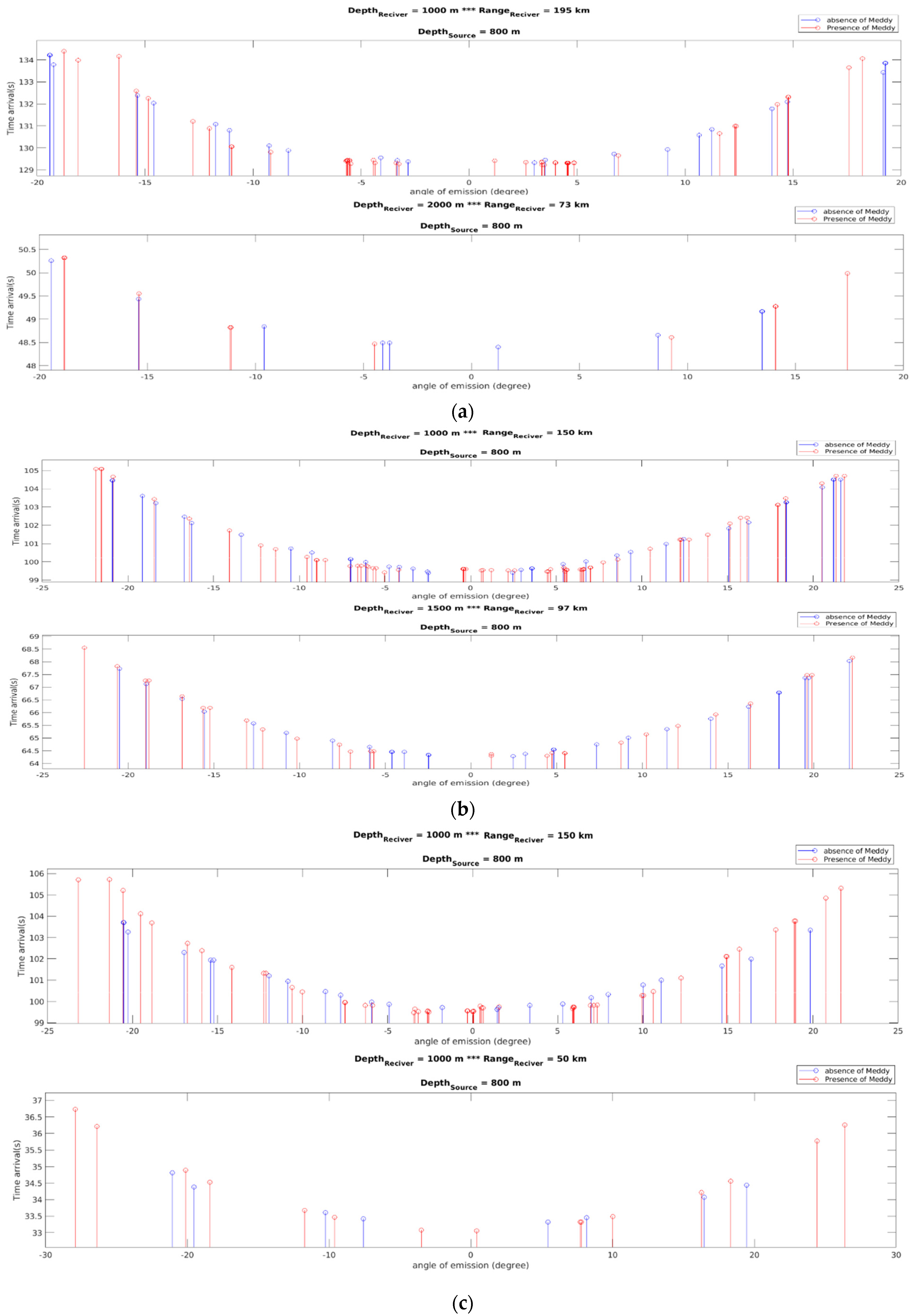
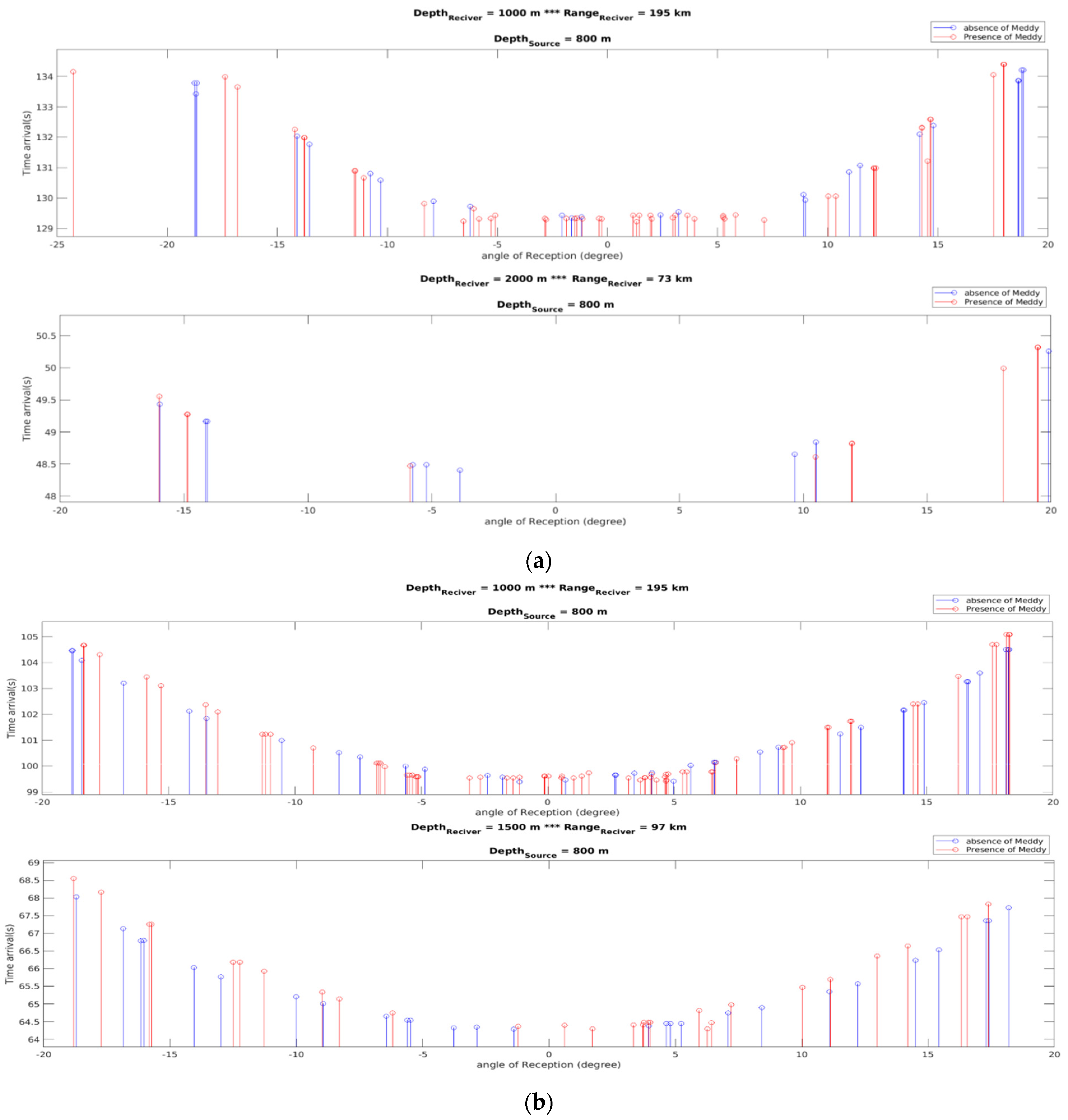
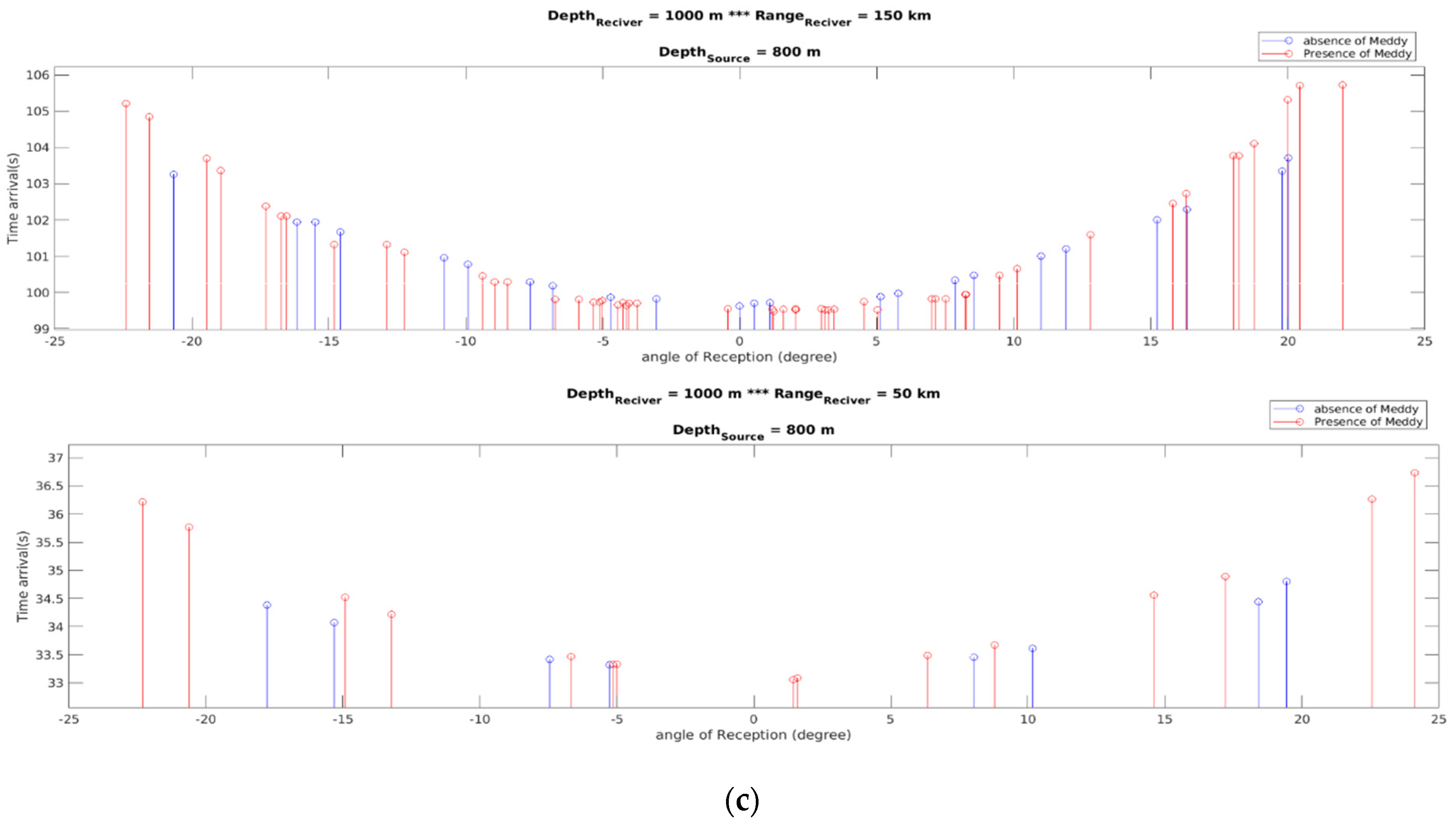
3.1.2. Number and Time of Arrival of Sound Signals at Different Receivers

To obtain more information on Meddy influence on sound propagation, synthetic receivers were placed at different depths (keeping the range constant) or at different ranges (keeping the depth constant) (see Figure A1, Figure A2 and Figure A3 in Appendix A). As mentioned before, the sound signals that do not reach the receiver are not shown on the plots. In this subsection, we analyze in detail the number and time of arrival of sound signals at the various receivers.

As a general remark, we note that more signals reached the receivers in the presence than in the absence of Meddy 33. We also note that, with Meddy 33, signals emitted with a wide angle (larger than ±10°) were reflected several times at the surface and at the bottom, and reached the receiver at a later time than those with a narrower angle of emission (see

Table A2. Number of sound signals reaching the receiver in the absence or presence of Meddy 33 on 9 June 2006 as a function of emission angle and reception angle.

Meddy (Date)		Number of Sound Signals Reaching the Receivers
	Name of Receiver (Depth of Receiver (m), Range of Receiver (km))	Emission Angles (−10° to 10°)		Emission Angles (−10° to −25° and 10° to 25°)		Reception Angles (−10° to 10°)		Reception Angles (−10° to −25° and 10° to 25°)
		Absence of Meddy	Presence of Meddy	Absence of Meddy	Presence of Meddy	Absence of Meddy	Presence of Meddy	Absence of Meddy	Presence of Meddy
Meddy 33 (9 June 2006)	1 (1000 m, 10 km)	2	2	3	3	2	2	3	3
	2 (1000 m, 50 km)	3	5	5	10	3	7	5	8
	3 (1000 m, 80 km)	7	10	8	12	7	11	8	11
	4 (11 m, 150 km)	4	6	17	33	8	12	13	27
	5 (11 m, 195 km)	18	18	11	34	18	23	11	29
	6 (600 m, 150 km)	11	28	13	23	12	31	12	20
	7 (2000 m, 150 km)	12	25	12	15	11	22	13	18

,

Table A3. Time of arrival of sound signals in the absence or presence of Meddy 33 on on 6 February 2004 and 28 January 2005 as a function of emission angle and reception angle.

Meddy (Date)		Mean Time of Arrival [s]
	Name of Receiver (Depth of Receiver (m), Range of Receiver (km))	Emission Angles (−10° to 10°)		Emission Angles (−10° to −25° and 10° to 25°)		Reception Angles (−10° to 10°)		Reception Angles (−10° to −25° and 10° to 25°)
		Absence of Meddy	Presence of Meddy	Absence of Meddy	Presence of Meddy	Absence of Meddy	Presence of Meddy	Absence of Meddy	Presence of Meddy
Meddy 33 (6 February 2004)	1 (2000 m, 10 km)	6.67	6.67	6.88	6.88	6.67	6.67	6.88	6.88
	2 (2000 m, 73 km)	48.58	48.54	49.50	49.55	48.51	48.47	49.37	49.44
	3 (2000 m, 100 km)	66.56	66.29	68.08	68.11	66.49	66.29	67.94	68.11
	4 (11 m, 195 km)	129.57	129.40	132.24	132.74	129.52	129.40	131.92	132.74
	5 (800 m, 195 km)	129.57	129.39	132.54	132.69	129.49	129.38	132.12	132.59
	6 (1000 m, 195 km)	129.65	129.38	132.58	132.16	129.65	129.38	132.58	132.16
	7 (2000 m, 195 km)	129.70	129.38	132.03	132.11	129.56	129.38	132.44	132.11
	8 (3200 m, 195 km)	129.84	129.41	132.60	132.67	129.99	129.41	132.87	132.17
Meddy 33 (28 January 2005)	1 (1000 m, 10 km)	6.63	6.66	7.34	7.24	6.63	6.66	7.34	7.24
	2 (1000 m, 70 km)	46.54	46.58	48.28	48.30	46.54	46.67	48.28	48.31
	3 (1000 m, 97 km)	64.54	64.47	66.56	66.58	64.54	64.61	66.56	66.89
	4 (11 m, 150 km)	99.96	99.65	102.49	102.65	99.96	99.80	102.49	103.26
	5 (500 m, 150 km)	99.73	99.63	102.66	102.26	99.73	99.69	102.66	102.51
	6 (1000 m, 150 km)	99.87	99.67	102.89	102.93	99.92	99.77	103.01	103.08
	7 (1500 m, 150 km)	99.80	99.69	103.00	102.83	99.85	99.76	103.12	103.30

,

Table A4. Time of arrival of sound signals in the absence or presence of Meddy 33 on 9 June 2005 as a function of emission angle and reception angle.

Meddy (Date)		Mean Time of Arrival (s)
	Name of Receiver (Depth of Receiver (m), Range of Receiver (km))	Emission Angles (−10° to 10°)		Emission Angles (−10° to −25° and 10° to 25°)		Reception Angles (−10° to 10°)		Reception Angles (−10° to −25° and 10° to 25°)
		Absence of Meddy	Presence of Meddy	Absence of Meddy	Presence of Meddy	Absence of Meddy	Presence of Meddy	Absence of Meddy	Presence of Meddy
Meddy 33 (9 June 2006)	1 (1000 m, 10 km)	6.64	6.63	7.37	7.37	6.64	6.63	7.37	7.37
	2 (1000 m, 50 km)	33.40	33.25	34.26	35.03	33.40	33.35	34.26	35.40
	3 (1000 m, 80 km)	53.38	53.14	54.77	55.41	53.38	53.19	54.77	55.57
	4 (11 m, 150 km)	100.38	99.65	102.30	103.52	100.77	100.34	102.80	104.08
	5 (11 m, 195 km)	99.87	99.69	101.97	103.03	99.87	99.87	101.97	103.46
	6 (600 m, 150 km)	99.99	99.69	102.14	102.81	100.05	99.76	102.25	103.17
	7 (2000 m, 150 km)	100.12	99.80	102.52	102.54	100.07	99.73	102.37	102.13

,

Table A5. Number of sound signals which reach the receiver in the absence or presence of Meddy 120, 135 and 143 as a function of the emission or reception angles.

Meddy (Date)		Number of Sound Signals Reaching the Receivers
	Name of Receiver (Depth of Receiver (m), Range of Receiver (km))	Emission Angles (−10° to 10°)		Emission Angles (−10° to −25° and 10° to 25°)		Reception Angles (−10° to 10°)		Reception Angles (−10° to −25° and 10° to 25°)
		Absence of Meddy	Presence of Meddy	Absence of Meddy	Presence of Meddy	Absence of Meddy	Presence of Meddy	Absence of Meddy	Presence of Meddy
Meddy 120 (9 December 2014)	1 (11 m,195 km)	8	16	20	20	12	20	16	16
	2 (500 m, 195 km)	27	45	20	20	26	45	21	20
	3 (1500 m, 195 km)	16	35	20	20	16	35	20	20
	4 (1500 m, 10 km)	2	2	3	4	1	2	4	4
	5 (1500 m, 68 km)	7	6	10	10	7	6	10	10
	6 (1500 m, 100 km)	6	16	13	13	6	17	13	12
Meddy 135 (25 January 2016)	1 (11 m, 185 km)	4	32	20	20	10	36	14	16
	2 (800 m, 185 km)	25	95	18	19	26	96	17	18
	3 (1200 m, 185 km)	20	98	17	16	21	99	16	15
	4 (1200 m, 10 km)	1	1	3	3	1	1	3	3
	5 (1200 m, 43 km)	4	3	9	9	4	3	9	9
	6 (1200 m, 100 km)	13	17	11	20	13	17	11	10
Meddy 143 (13 May 2017)	1 (11 m, 195 km)	8	21	29	40	11	28	26	33
	2 (800 m, 195 km)	18	60	35	39	18	62	35	37
	3 (1500 m, 195 km)	17	57	46	53	17	58	46	52
	4 (1500 m, 10 km)	1	1	3	3	1	1	3	3
	5 (1500 m, 62 km)	4	4	12	11	4	4	12	11
	6 (1500 m, 100 km)	7	15	17	20	7	16	17	19

and

Table A6. Time of arrival of sound signals in the absence and presence of Meddy 120 and Meddy 135, as a function of emission angle and of reception angle.

Meddy (Date)		Mean Time of Arrival (s)
	Name of Receiver (Depth of Receiver (m), Range of Receiver (km))	Emission Angles (−10° to 10°)		Emission Angles (−10° to −25° and 10° to 25°)		Reception Angles (−10° to 10°)		Reception Angles (−10° to −25° and 10° to 25°)
		Absence of Meddy	Presence of Meddy	Absence of Meddy	Presence of Meddy	Absence of Meddy	Presence of Meddy	Absence of Meddy	Presence of Meddy
Meddy 120 (9 December 2014)	1 (11 m, 195 km)	130.26	129.86	133.69	133.65	130.64	130.16	134.26	134.22
	2 (500 m, 195 km)	129.76	129.65	133.69	133.65	129.73	129.65	133.55	133.65
	3 (1500 m, 195 km)	129.90	129.74	133.69	133.67	129.90	129.74	133.69	133.67
	4 (1500 m, 10 km)	6.65	6.65	7.25	7.25	6.65	6.65	7.25	7.25
	5 (1500 m, 68 km)	45.31	45.25	47.13	47.10	45.31	45.25	47.13	47.10
	6 (1500 m, 100 km)	66.66	66.46	69.00	68.94	66.66	66.50	69.00	69.09
Meddy 135 (25 January 2016)	1 (11 m, 185 km)	123.89	123.21	126.84	126.81	124.65	123.40	127.56	127.27
	2 (800 m, 185 km)	123.27	123.01	127.16	127.28	123.32	123.02	127.31	127.44
	3 (1200 m, 185 km)	123.33	122.95	127.22	127.17	123.39	122.97	127.38	127.35
	4 (1200 m, 10 km)	6.64	6.64	7.35	7.34	6.64	6.64	7.35	7.34
	5 (1200 m, 43 km)	28.66	28.65	30.49	30.47	28.64	28.65	30.49	30.47
	6 (1200 m, 100 km)	66.63	66.57	68.95	68.69	66.63	66.57	68.95	68.69
Meddy 143 (13 May 2017)	1 (11 m, 195 km)	130.14	129.68	133.22	133.10	130.47	130.07	133.44	133.50
	2 (800 m, 195 km)	129.84	129.50	132.81	132.73	129.84	129.53	132.81	132.84
	3 (1500 m, 195 km)	129.82	129.50	132.56	132.27	129.82	129.52	132.56	132.30
	4 (1500 m, 10 km)	6.65	6.65	7.40	7.40	6.65	6.65	7.40	7.40
	5 (1500 m, 62 km)	41.35	41.32	42.64	42.53	41.35	41.32	42.64	42.53
	6 (1500 m, 100 km)	66.63	66.39	68.13	68.12	66.63	66.44	68.13	68.18

in Appendix B), which give the number of sound signals reaching the receivers in the presence or absence of Meddy 33). Conversely, signals with small emission angles (between −11° to 11°) reached the receivers earlier in the presence of Meddy 33 than in its absence; in the former case, they propagated in the sound channel. They were strong because their transmission loss was low, and they moved directly towards the receiver (see again

Table A1. Number of sound signals reaching the receiver in the absence or presence of Meddy 33 on 6 February 2004 and 28 January 2005 as a function of emission and reception angles.

Meddy (Date)		Number of Sound Signals Reaching the Receivers
	Label of Receiver (Depth (m), Range (km))	Emission Angles (−10° to 10°)		Emission Angles (−10° to −25° and 10° to 25°)		Reception Angles (−10° to 10°)		Reception Angles (−10° to −25° and 10° to 25°)
		Absence of Meddy	Presence of Meddy	Absence of Meddy	Presence of Meddy	Absence of Meddy	Presence of Meddy	Absence of Meddy	Presence of Meddy
Meddy 33 (6 February 2004)	1 (2000 m, 10 km)	1	1	1	1	1	1	1	1
	2 (2000 m, 73 km)	5	2	4	8	4	1	5	9
	3 (2000 m, 100 km)	3	6	9	10	2	6	10	10
	4 (11 m, 195 km)	17	19	12	17	15	19	14	17
	5 (800 m, 195 km)	22	41	15	28	19	40	18	29
	6 (1000 m, 195 km)	9	28	15	22	10	30	14	20
	7 (2000 m, 195 km)	8	22	16	30	6	22	18	30
	8 (3200 m, 195 km)	6	30	18	31	8	30	16	31
Meddy 33 (28 January 2005)	1 (1000 m, 10 km)	1	1	5	4	1	1	5	4
	2 (1000 m, 70 km)	9	9	12	12	9	11	12	10
	3 (1000 m, 97 km)	13	12	14	17	13	15	14	14
	4 (11 m, 150 km)	13	25	13	17	13	29	13	13
	5 (500 m, 150 km)	21	75	17	28	21	79	17	24
	6 (1000 m, 150 km)	17	42	19	27	18	46	18	23
	7 (1500 m, 150 km)	18	46	20	16	19	49	19	13

, Table A2, Table A3 and Table A4 in Appendix B which show the time of arrival of the signals).

Now, we consider the case of several receivers at the same range but at different depths. On 6 February 2004, the times of arrival of all signals in the absence of the Meddy ranged from 129 s to 134.2 s, and, in the presence of the Meddy, between 129 s and 134.5 s. At this date, the sound speed was low at the surface (about 1508 m/s), and the signals reached the surface and reflected on it, increasing their time of arrival at the receiver. However, on 9 June 2006 (see Table A2 in Appendix B), most sound signals reaching the receiver had a large emission angle (larger than ±11°). On this day, the times of arrival in the absence of the Meddy ranged between 99.5 s to 104.5 s, and in the presence of the Meddy, times of arrival ranged between 99.5 s to 105.5 s. This increased on 28 January 2005: in the absence of the Meddy, it ranged from 99.5 s to 103.9 s, and in the presence of the Meddy, times of arrival ranged between 99.5 s to 105.9 s. This was due to the high sound speed at the surface, which prevented most of the signals from reaching it. In the presence of the Meddy, the modified sound speed at depths between 1000 and 2500 m made these sound signals reach the receiver later.

Now, we consider the case of several receivers placed at the same depth but at different ranges. Signals reaching close receivers (10 km away from the source) are the fewest at all 3 dates, because near the source, the signals propagate towards the surface or the bottom after being emitted. Their times of arrival in the absence or presence of the Meddy are almost the same (see the Figure A7 in the Appendix A). However, as the range increases, more sound signals are received in both cases (absence or presence of the Meddy). Notwithstanding a few exceptions, we can state that the presence of Meddy 33 could be inferred from the delayed arrival of signals emitted at wide angles.

The time of arrival is analyzed with respect to the angle of reception. As was mentioned before, more sound signals reached the receivers in the presence of Meddy 33 than in its absence. Late (respectively, early) sound signals reached the receivers at large (respectively, small) angles since they are reflected at the bottom and at the surface (see Figure A8 in Appendix A). Furthermore, in the presence of the Meddy, most sound signals reached the receivers at small angles (between −10° to 10°), and they had short times of arrival (99 s, 100 s and 129 s). Again, this clearly characterizes the influence of the Meddy in the number of sound rays and on their time of arrival.

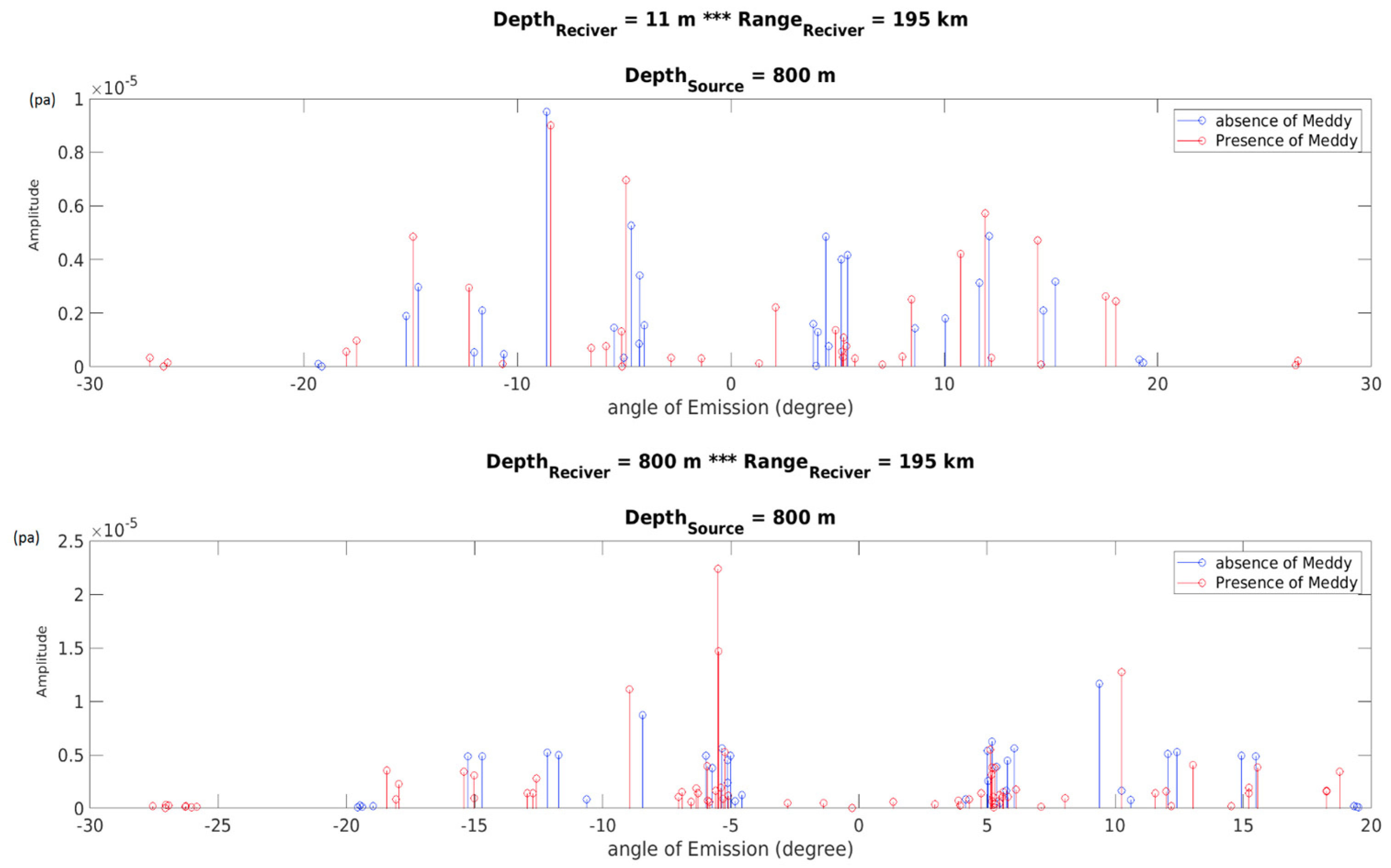
3.1.3. The Pressure Amplitude of Sound Signals at Various Receivers

The presence of the Meddy affects the pressure amplitude of the sound signals received. No universal pattern was observed for the pressure amplitude. Generally, the largest amplitudes were found for narrow angles of emission and of reception. Signals emitted at a wider angle underwent more reflections and were weaker (see Figure A9 in the Appendix A).

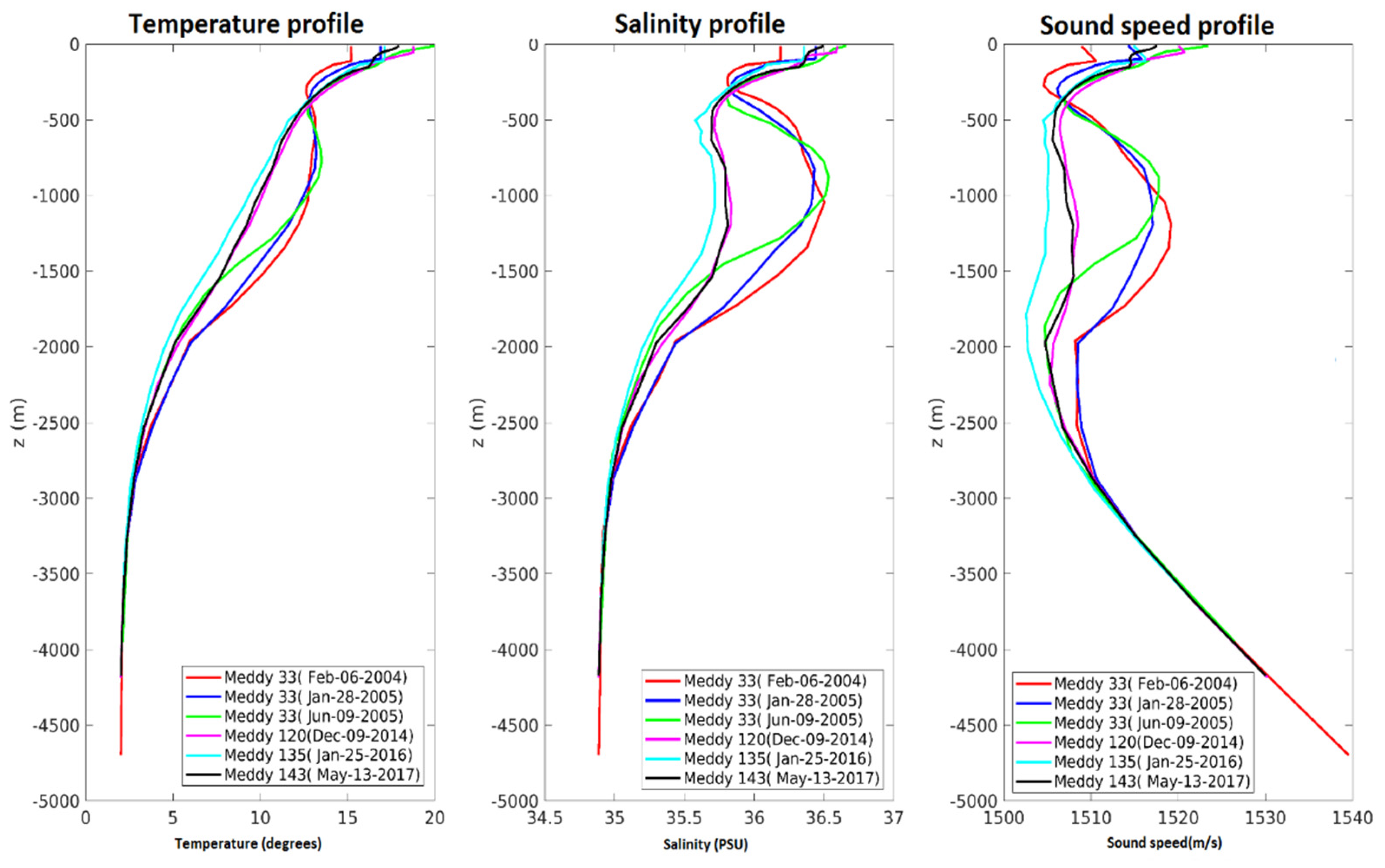
3.2. Acoustic Impact of the Other Meddies

As a further analysis, three additional Meddies were chosen, and their impact on sound signals were investigated. In particular, we analyzed:

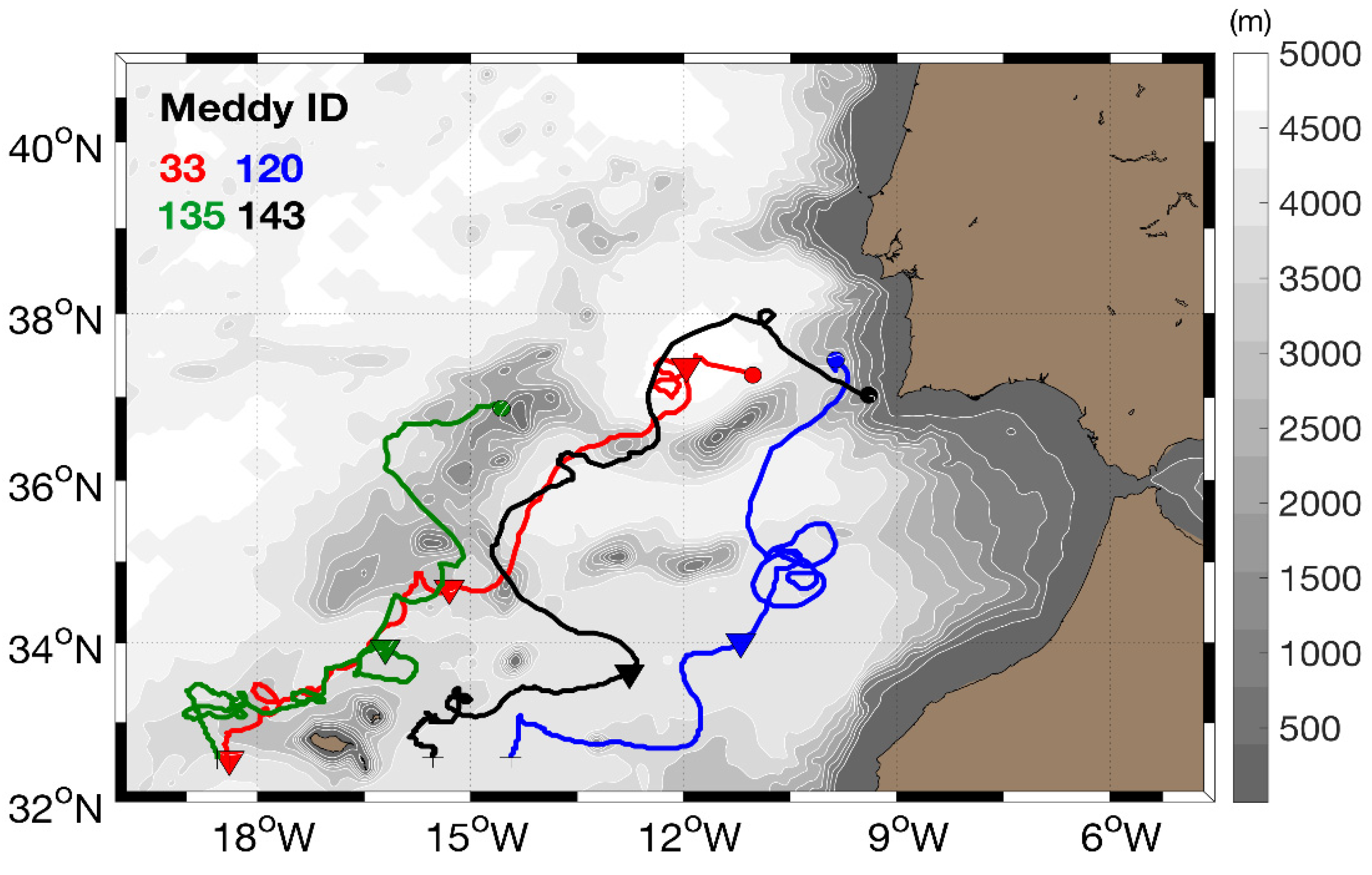
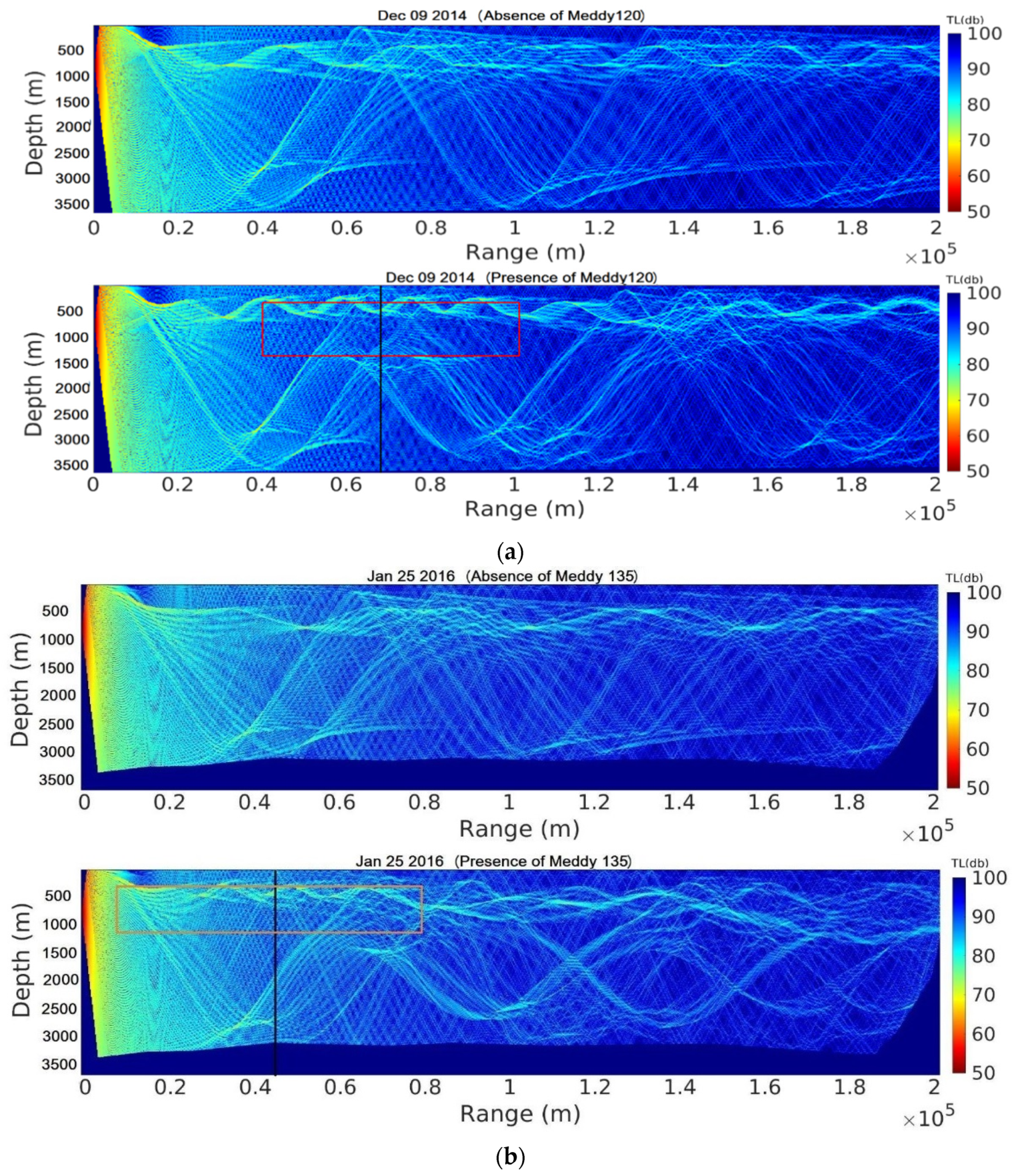
• The case of Meddy 120: this Meddy was tracked for 27 months and was first detected on 27 July 2013. Its radius and swirl velocity ranged from 10 to 35 km and 16 to 29 cm/s;
• The case of Meddy 135: this Meddy was tracked for 34 months and was first detected on 16 March 2013. Its radius and swirl velocity ranged from 18 to 43 km and 14 to 33 cm/s;
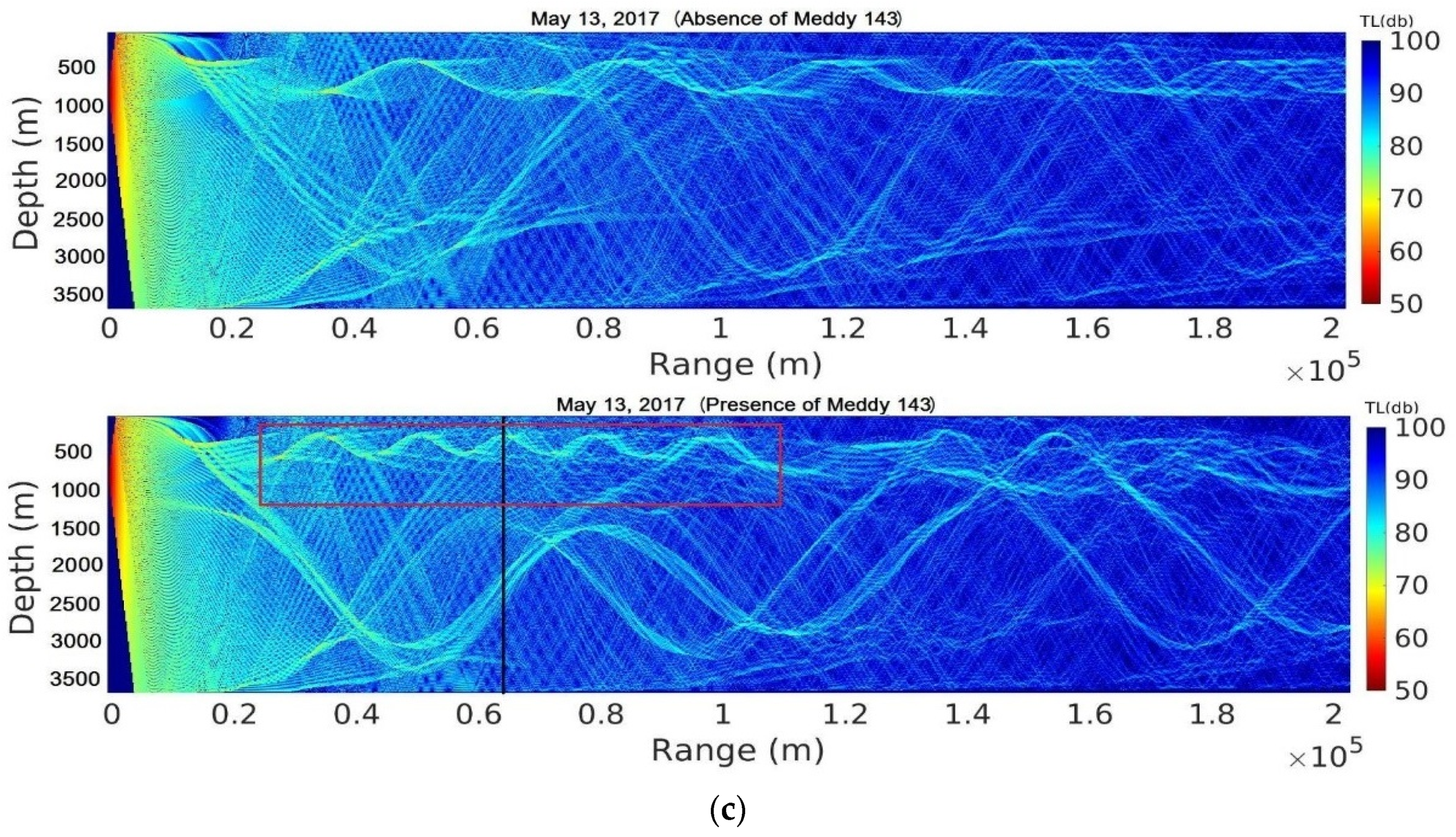
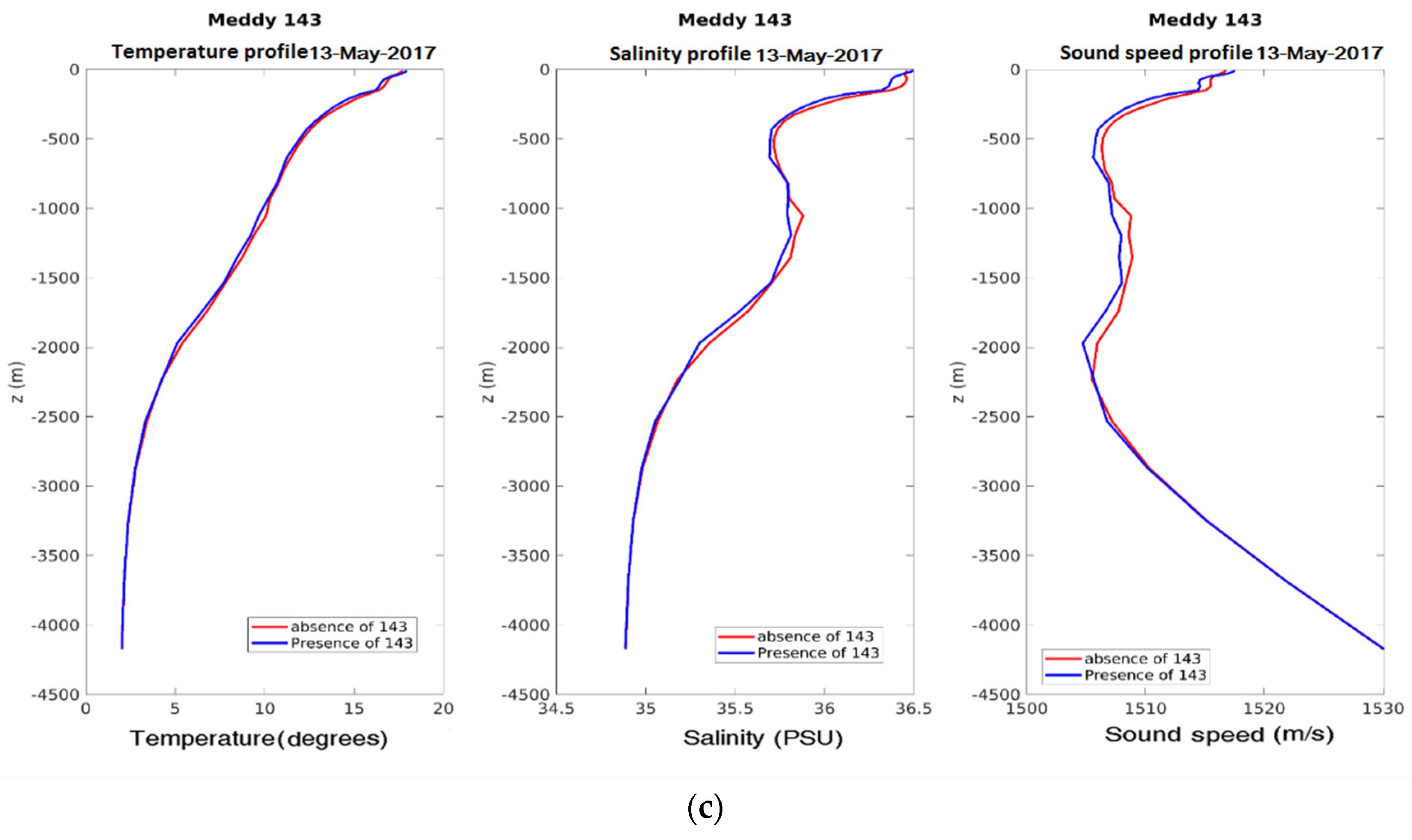
• The case of Meddy 143: this Meddy was tracked for 29 months and was first detected on 24 December 2013. Its radius and swirl velocity ranged from 17 to 44 km and 12 to 31 cm/s;

The vertical profiles of temperature, salinity and sound speed showed the following results (see Figure A10 in the Appendix A). In all Meddies, the sound speed at the surface was between 1515 to 1520 m/s, i.e., larger than the values observed at depths down to 3500 m. The Meddy hydrodynamical structure thus impacted sound signals and created a sound channel (between 300 m and 600 m depth).

In the presence of Meddy 120, the sound speed was high at the surface (about 1520 m/s) and decreased to nearly 1505 m/s at depths of 2200 m, a larger sound speed difference compared to the other two Meddies. For Meddy 135, the sound speed decreased from the surface (about 1517 m/s) down to 2000 m, where it reached its minimal value (about 1504 m/s). At depths of about 300 m as well as between 2500 m and the bottom, in the absence of Meddy 135, the sound speed was greater than in the presence of the Meddy. For Meddy 143, the sound speed was 1519 m/s at the surface, which was greater than outside of the Meddy (about 1517 m/s). The sound speed decreased and reached a minimum around 2000 m (about 1505 m/s in the Meddy). This vertical decrease of sound speed (from the surface to the 2000 m depth) in the presence of Meddy 143 was larger than in its absence (changing vertically and smoothly between 500 to 2000 m).

Figure 7 shows the sound speed profiles for the analyzed Meddies within their core. Compared with Meddy 33, the sound speed profiles of Meddy 120, 135 and 143 at mid-depth (between 500 to 2000 m) were lower and changed more smoothly. In Meddy 33, the minimum value of sound speed occurred at 400 m, but in other Meddies, the sound speed reached its minimum value at about 2000 m.

3.2.1. The Sound Propagation and the Transmission Loss of Sound Signals

Here we investigate the propagation and transmission loss of sound signals for Meddy 120, 135 and 143 using the same methodology adopted for Meddy 33. The depth of the source (Ds) is 800 m and the source frequency is 200 Hz. The acoustic range for all the Meddies is 201 km. Sound signals are emitted with angles between −35° to 35°, and in all Meddies, most signals are reflected between the bottom and the surface (bathymetry is included).

Figure 8 shows the transmission loss and the propagation of sound signals at all dates (see also Table A5 and Table A6 in Appendix B). In all three Meddies, most of the signals which are emitted at large angles are reflected by the surface and bottom. In the absence of Meddies, we observe a surface sound channel. However, few sound signals moved along a straight line within the acoustic range and in the sound channel. As the range increased, the sound signal energy decreased due to the reflection between the ocean surface and bottom.

In the presence of the Meddies, the depth of the surface sound channel decreased and reached 500 m. At the location of the Meddies, their hydrological structure led to the creation of a deep sound channel between 1500 m and 3500 m. The number of sound signals moving in a straight line along the acoustic range and in both sound channels increased. The sound signals were stronger at the location of the Meddies, and the transmission loss decreased.

The following behavior is observed for all Meddies: the presence of Meddies caused the creation of 2 sound channels in which the sound signals were more intense because their transmission loss decreased (it reached 80–85 dB). After crossing the Meddies, the sound signals in the two sound channels deviated and scattered or mixed with each other.

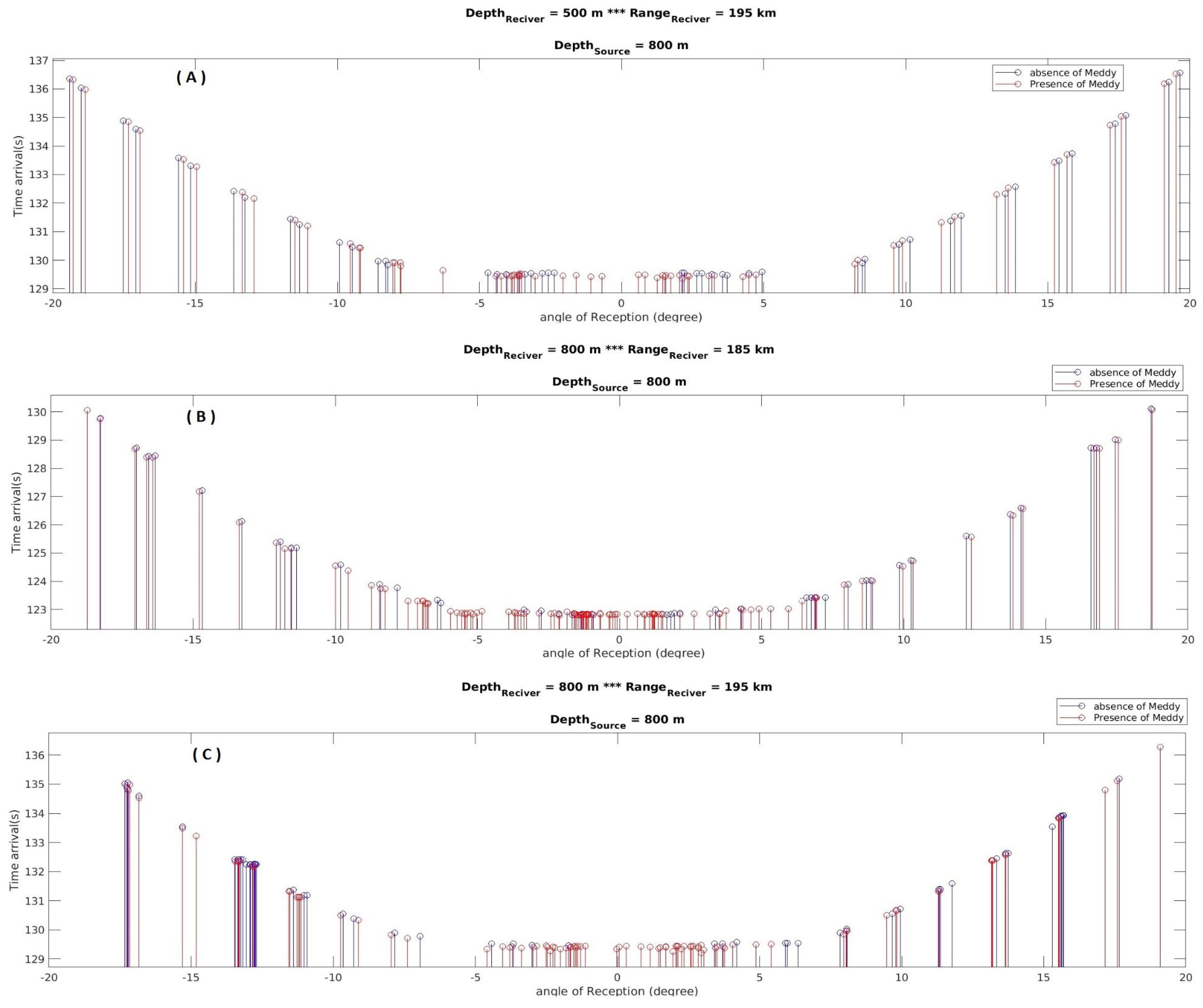
3.2.2. The Number and Time of Arrival of Sound Signals at Different Receivers

For the additional Meddies analyzed here, three receivers were placed at different depths (keeping the range constant), and three receivers were positioned at different ranges (keeping the depth constant). The sound propagation was investigated both in the presence and in the absence of the Meddies. Figure A11 and Figure A12 in the Appendix A show the time of arrival of sound signals as a function of the angle of emission and as a function of the receiving angle, respectively (see also the Table A5 and Table A6 in Appendix B).

In the presence of the Meddies, more signals reached the receivers than in their absence. A majority of sound signals which reached the receivers had small angles of emission (between −10° and 10°) and shorter times of arrival (between 123 s and 129 s). More signals were received at long range.

With Meddies 135 and Meddy 143, the time of arrival in the absence of the Meddy was larger than in the unperturbed case. The range of values of the time of arrival in Meddy 120 was larger than for other Meddies (relatively between 129.5 s to 136.5 s) and close to that of Meddy 143. Finally, the range of values of the time of arrival for Meddy 135 was smaller than for other Meddies (relatively between 123 s to 130 s).

In investigating the time of arrival as a function of the angle of reception, it was observed that in the presence of Meddies, the number of sound signals with low angles reaching the receiver increases, generating positive differences from 2 to 10. Most of them arrive at the small angle. In the absence of Meddy 143, most of the sound signals reach the receivers at large angles.

4. Discussion and Conclusions

In the present work, the effect of Meddies on sound propagation was investigated. The aim of this study was to determine and characterize the acoustic signature of Meddies, so that this can be inverted in order to retrieve their hydrological structure. For this purpose, four Meddies with long lifetimes were selected using the output of the ROMS numerical model; the sound propagation was studied (along a vertical cross-section) in the presence or absence of Meddies using the Bellhop model. To investigate the sound signals, we considered the domain to be 201 km in range, bounded at the bottom by the local bathymetry; the depth of the sound source was chosen to be 800 m, its frequency was 200 Hz and the angle of emission was between −35° and 35°.

The main questions in this paper introduction were: (1) Do Meddies in general create a characteristic change in sound propagation (e.g., compared with surface vortices)? (2) Do significantly different Meddies create very distinct acoustic changes (that could be inverted in order to retrieve the hydrological structure of the Meddies)?

To answer the first question, we have analyzed 6 different cases of Meddies, among which 3 cases were Meddy 33 at 3 different stages of its lifetime and 3 other cases were Meddies 120, 135, and 143. These Meddies’ features are representative of typical Meddies observed in the North Atlantic and provide enough diversity so that the results presented here can be generalised.

Firstly, we observed that the sound speed was higher in the presence than in the absence of a Meddy, an effect which was due to the formation of new sound channels or to the change in depth of existing ones, which in turn modified the energy and time of arrival of the acoustic signals.

The observed changes can be first classified in terms of sound channels (i.e., vertically). If the sound speed at the surface was lower than that of mid-depth (between 1500 to 3000 m), the sound signals with different angles of emission can reach the surface easily or move in the surface sound channel. If the sound speed at the surface was larger than at mid-depth, the sound propagation near the surface would be more difficult and only two types of sound signals could reach the surface: the reflected sound signals from the bottom and the large angle of emission sound signals (angles larger than −20° or +20°). Nevertheless, these wide-angle signals would not reach the receivers at long ranges because of a large transmission loss.

Secondly, the horizontal changes in sound propagation in the presence of the Meddy focus sound propagation in its vicinity. Near Meddy 33, sound signals propagated with little energy losses across the shallow and narrow sound channel. Sound signals deviated downwards after passing the Meddy. The presence of Meddies can generate sound channels, decrease transmission loss and promote sound transmission.

The times of arrival of the acoustic signals at the receivers were investigated as a function of the angle of emission and as a function of the angle of reception. Note that, obviously, the times of arrivals were larger for wide angles of emission (leading to multiple reflections at the surface and at the bottom). These effects were general for all Meddies: they were observed at the mid-life of Meddy 33 (28 January 2005), at the end of its life (9 June 2006) and also for the three other Meddies (Meddy 120, 135, and 143).

The changes in acoustic signal propagation in the presence of Meddies are also different from those in the presence of surface eddies, as described in previous studies.

To answer the second question, we considered the time of arrival and energy of acoustic signals for all Meddies. To obtain sufficient information, we used several receivers at the same range and different depths, and conversely at the same depth and at different ranges. Clearly, for different Meddies, with different hydrological structures, the acoustic impact was different: indeed, 3 factors, the bottom depth in the area, the sound speed at the surface, and the sound speed at intermediate depths (between 1000 and 3000 m), affect the time of arrival of the sound signals. Meddies affect the sound propagation as well as the time of arrival by changing the last two factors (sound speed at the surface and at mid-depth). When the sound speed is low at the surface, the sound signals can reach the surface, and this affects the time of arrival of sound signals to the receivers. The smaller the difference between the sound speed in the case with and without a Meddy, the closer the time of arrival of sound signals for the two modes. When the sound speed is high at the surface, changes in sound speed at mid-depths affect the signal’s time of arrival. The greater the difference between the sound speed in the mid-depth, the greater the difference between the times of arrival. The depth of the area (obviously, not Meddy-dependent) also affects the amount of time the signals take to reflect between the surface and the bottom.

Our study has essentially considered Meddies (i.e., deep anticyclones of Mediterranean Water), and even more precisely, Meddies in isolation from other motions, to calculate their acoustic impact. Further work should concentrate on the impact of deep cyclones of Mediterranean Water, on the association of several Meddies, of Meddies with filaments or of Meddy interaction with internal waves. Of interest also are the other submesoscale subsurface eddies in the world oceans, like Reddies (Red Sea Water eddies), Peddies (Persian Gulf Water eddies), Leddies (Levantine Intermediate Water eddies), etc. Another development of this study could be passive acoustics where ambient noise is used to track the subsurface eddies, but for the moment, the impact of such eddies on sound speed is complex enough that using a well-controlled acoustic source is still necessary.

The result of this study is the first step of a project in which we wish to establish the relationship between sound signals and Meddy parameters in order to be able to detect Meddies. The analysis of the effect of different meddies on sound signals showed us that Meddies with different characteristics (radius, depth, thickness and speed) can have different effects on sound signals. By considering the Meddy parameters (thickness, radius, speed, and etc.) and the characteristics of the sound signals (time of arrival, angle of reception, sound speed, and transmission loss), one can establish a relation between Meddy parameters and sound characteristics. The complementarity of the acoustic and of surface dynamical information (sea surface height anomalies related to the eddy) will also be investigated. Using neural networks, the relation between subsurface eddy structure and their various signatures can be inferred, in particular for typical eddies of the Northeastern Atlantic Ocean. The results of the present study will contribute to the data needed by the neural networks. Finally, the impact of eddies in the presence of other flow structures (internal waves, oceanic turbulence), rendering the problem more stochastic, will also be addressed.

References

1. Maia, L.P.; Carriere, O.; Parente, C.E.; Hermand, J.P. Acoustic inversion with a frequency-domain version of the model-based matched filter processing. In Proceedings of the European Conference on Underwater Acoustics, Istanbul, Turkey, 5–9 July 2010. [Google Scholar]
2. Lermusiaux, P.F.J.; Haley, P.J.; Mirabito, C.; Ali, W.H.; Bhabra, M.; Abbot, P.; Chiu, C.S.; Emerson, C. Multi-resolution Probabilistic Ocean Physics-Acoustics Modeling: Validation in the New Jersey Continental Shelf. In Proceedings of the Global Oceans Conference, Singapore, 5–31 October 2020. [Google Scholar] [CrossRef]
3. Chen, X.; Hong, M.; Zhu, W.; Mao, K.; Ge, J.J.; Bao, S. The analysis of acoustic propagation characteristics affected by mesoscale cold-core vortex, based on the UMPE model. Acoust. Aust. 2019, 47, 33–49. [Google Scholar] [CrossRef]
4. Li, J.; Zhang, R.; Liu, C.; Fan, H. Modeling of ocean mesoscale eddy and its application in the underwater acoustic propagation. Mar. Sci. Bull. 2012, 14, 1–15. [Google Scholar]
5. Chelton, D.B.; Schlax, M.G.; Samelson, R.M. Global observations of nonlinear mesoscale eddies. Prog. Oceanogr. 2011, 91, 167–216. [Google Scholar] [CrossRef]
6. De Marez, C.; Carton, X.; L’Hégaret, P. Oceanic vortex mergers are not isolated but influenced by the β-effect and surrounding eddies. Sci. Rep. 2020, 10, 1–10. [Google Scholar] [CrossRef] [PubMed] [Green Version]
7. De Marez, C.; Carton, X.; Corréard, S.; L’Hégaret, P.; Morvan, M. Observations of a deep submesoscale cyclonic vortex in the Arabian Sea. Geophys. Res. Lett. 2020, 47, e2020GL087881. [Google Scholar] [CrossRef]
8. Zhang, Z.; Wang, W.; Qiu, B. Oceanic mass transport by mesoscale eddies. Science 2014, 345, 322–324. [Google Scholar] [CrossRef]
9. Dong, C.; McWilliams, J.C.; Lu, Y.; Chen, D. Global heat and salt transports by eddy movements. Nat. Commun. 2014, 5, 1–6. [Google Scholar] [CrossRef] [PubMed] [Green Version]
10. L’Hegaret, P.; Duarte, R.; Carton, X.; Vic, C.; Ciani, D.; Baraille, R.; Correard, S. Mesoscale variability in the Arabian Sea from HYCOM model results and observations: Impact on the Persian Gulf Water path. Ocean Sci. 2015, 11, 667–693. [Google Scholar] [CrossRef] [Green Version]
11. Wang, Y.; Li, C.; Liu, Q. Observation of an anti-cyclonic mesoscale eddy in the subtropical northwestern Pacific Ocean from altimetry and Argo profiling floats. Acta Oceanol. Sin. 2020, 39, 79–90. [Google Scholar] [CrossRef]
12. Henrick, R.; Jacobson, M.; Siegmann, W. General effects of currents and sound-speed variations on short-range acoustic transmission in cyclonic eddies. J. Acoust. Soc. Am. 1980, 67, 121–134. [Google Scholar] [CrossRef]
13. Bong-Chae, K.; Kyoung Choi, C.; Byoung-Nam, K. Influence of a Warm Eddy on Low-frequency Sound Propagation in the East Sea. Ocean Polar Res. 2012, 34, 325–335. [Google Scholar]
14. Lawrence, M. Modeling of acoustic propagation across warm-core eddies. J. Acoust. Soc. Am. 1983, 73, 474–485. [Google Scholar] [CrossRef]
15. Qingyu, L. Sound Propagation under the Mesoscale Ocean Phenomena. Ph.D. Thesis, Harbin Engineering University, Harbin, China, 2006. [Google Scholar]
16. Baer, R.N. Calculations of sound propagation through an eddy. J. Acoust. Soc. Am. 1980, 67, 1180–1185. [Google Scholar] [CrossRef]
17. Swallow, J. A deep eddy off Cape st. Vincent. Deep-Sea Res. 1969, 16, 285–295. [Google Scholar]
18. Armi, L.; Hebert, D.; Oakey, N.; Price, J.F.; Richardson, P.L.; Rossby, H.T.; Ruddick, B. Two years in the life of a Mediterranean salt lens. J. Phys. Oceanogr. 1989, 19, 354–370. [Google Scholar] [CrossRef]
19. Barbosa Aguiar, A.C.; Peliz, A.; Carton, X. A census of Meddies in a long-term high-resolution simulation. Prog. Oceanogr. 2013, 116, 80–94. [Google Scholar] [CrossRef] [Green Version]
20. Bashmachnikov, I.; Neves, F.; Calheiros, T.; Carton, X. Properties and pathways of Mediterranean water eddies in the Atlantic. Prog. Oceanogr. 2015, 137, 149–172. [Google Scholar] [CrossRef]
21. Shchepetkin, A.F.; Mcwilliams, J.C. The regional oceanic modeling system (ROMS): A split-explicit, free-surface, topography-following-coordinate oceanic model. Ocean Model 2005, 9, 347–404. [Google Scholar] [CrossRef]
22. Da Silva, A.; Young, A.C.; Levitus, S. Atlas of Surface Marine Data: Algorithms and Procedures; Number 6, COADS, NCAR/UCAR Data Archive; U.S. Department of Commerce: Washington, DC, USA, 1994; Volume 1.
23. Nencioli, F.; Changing, D.; Dickey, T.; Washburn, L.; McWilliams, J. A vector geometry-based Eddy Detection Algorithm and Its Application to a High-Resolution Numerical Model Product and High-Frequency Radar Surface Velocities in the Southern California Bight. J. Atmos. Ocean Technol. 2010, 27, 564–579. [Google Scholar] [CrossRef]
24. Richardson, P.L.; Bower, A.S.; Zenk, W. A census of Meddies tracked by floats. Prog. Oceanogr. 2000, 45, 209–250. [Google Scholar] [CrossRef]
25. Ciani, D.; Carton, X.; Barbosa Aguiar, A.C. Surface signature of Mediterranean water eddies in a long-term high-resolution simulation. Deep-Sea Res. Part I Oceanogr. Res. Pap. 2017, 130, 12–29. [Google Scholar] [CrossRef] [Green Version]
26. De Sousa Costa, E.; Medeiros, E. Numerical modeling and simulation of acoustic propagation in shallow water. Mecânica Comput. Acional. 2010, 29, 2215–2228. [Google Scholar]
27. Maggi, A.L.; Duncan, A.J. AcTUO v2.2 1—Acoustic Toolbox User-interface and Post-Processor, Installation and User Guide; Curtin University of Technology, Centre for Marine Science and Technology: Bentley, WA, Australia, 2006. [Google Scholar]
28. Mackenzie, K.V. Nine equation for Sound Speed in the Oceans. J. Acoust. Soc. Am. 1981, 33, 1498–1504. [Google Scholar] [CrossRef]
29. Khan, S.; Song, Y.; Huang, J.; Piao, S. Analysis of Underwater Acoustic Propagation under the Influence of Mesoscale Ocean Vortices. J. Mar. Sci. Eng. 2021, 8, 799. [Google Scholar] [CrossRef]
30. Hassantabar Bozroudi, S.H.; Mohammad Mehdizadeh, M.; Akbarinasab, M. Investigation of the loss of sound signals in the presence of Eddy in a hypothetical area. J. Mar. Eng. 2021, 17, 123–133. [Google Scholar]
Figure 1. Trajectories of the Meddies 33 (red), 120 (blue), 135 (green) and 143 (black) evolving through the study area. Circles and crosses respectively indicate the first and last detection of each Meddy. The triangles indicate the position of the analyses based on the ACTUP model. The grey contours are the bathymetry and brown areas are land.
Water 13 03617 g001
Figure 2. Sound speed versus depth and longitude for Meddy 33 on 7 August 2004. Meddy 33’s location is 13 w and 1000 m. The white areas are the bathymetry (seamounts) and land. The black square identifies the Mediterranean undercurrent.
Water 13 03617 g002
Figure 3. Hovmoller diagram showing the evolution of sound speed through Meddy 33′s center and along its trajectory (red line in Figure 1). Time is shown along the x-axis, while depth is shown along the y-axis. The white area at the bottom of the plot indicates the local and instantaneous height of bottom topography.
Water 13 03617 g003
Figure 4. Meddy 33 at its early life (6 February 2004), mid-term evolution (28 January 2005) and at its latest detection (9 June 2006). (a) The Meddy is identified via the ERTEL PV anomaly at 1000 m depth in the three panels superimposed to the trajectory image. The red line is the Meddy trajectory, the green point is the Meddy center (point called B), the grey contours are the bathymetry and brown areas are land. (b) The selected points (inside and outside the Meddy) are superimposed on the EPVA maps at the three dates. Point A (the black one) is chosen in the Meddy periphery and point B (the green one) is at the Meddy center. 6 February 2004: B has coordinates 37.35° N, 11.96° W and A has coordinates 38.5° N, 11.96° W (128 km from the center of the Meddy), 28 January 2005: B lies at 34.67° N, 15.29° W and A lies at 35.2° N, 15.29° W (59 km from the center of the Meddy) and 9 June 2006: B lies at 32.53° N, 18.39° W and A lies at 32.95° N, 18.39° W (47 km from the center of the Meddy).
Water 13 03617 g004
Figure 5. Vertical profiles of temperature (left), salinity (middle), and sound speed (right). The red line refers to the point outside the Meddy and the blue line to the Meddy core. (a) On 6 February 2004; (b) on 28 January 2005; (c) on 9 June 2006.
Water 13 03617 g005aWater 13 03617 g005b
Figure 6. The transmission loss of sound signals in the absence of the Meddy (top picture) and the presence of the Meddy (bottom picture), with Meddy location (framed in red) (a) on 6 February 2004; (b) on 28 January 2005; (c) on 9 June 2006.
Water 13 03617 g006aWater 13 03617 g006b
Figure 7. Vertical profile of temperature (left), salinity (middle), and sound speed (right) at the center of all of the Meddies.
Water 13 03617 g007
Figure 8. The transmission loss of sound signals in the absence of Meddy 120 (top) and in its presence (bottom), with Meddy location (framed in red) (a) on 9 December 2014; (b) on 25 January 2016; and (c) on 13 May 2017.
Water 13 03617 g008aWater 13 03617 g008b
Publisher’s Note: MDPI stays neutral with regard to jurisdictional claims in published maps and institutional affiliations.