Characteristics of the Water Vapor Transport in the Canyon Area of the Southeastern Tibetan Plateau

Abstract

Changes in the surface fluxes cause changes in the annular flow field over a region, and they affect the transport of water vapor. To study the influence of the changes in the surface flux on the water vapor transport in the upper layer in the canyon area of southeastern Tibet, in this study, the water vapor transport characteristics were analyzed using the HYSPLIT_v4 backward trajectory model at Danka and Motuo stations in the canyons in the southeastern Tibetan Plateau from November 2018 to October 2019. Then, using ERA-5 reanalysis data from 1989 to 2019 and the characteristics of the high-altitude water vapor transportation, the impact of the surface flux changes on the water vapor transportation was analyzed using singular value decomposition (SVD). The results show that the main sources of the water vapor in the study area were from the west and southwest during the non-Asian monsoon (non-AMS), while there was mainly southwest air flow and a small amount of southeast air flow in the lower layer during the Asian monsoon (AMS) at the stations in southeastern Tibet. The water vapor transmission channel of the westward airflow is higher than 3000 m, and the water vapor transmission channel of the southwestward and southeastward airflow is about 2000 m. The sensible heat and latent heat are negatively correlated with water vapor flux divergence. The southwest boundary of southeastern Tibet is a key area affecting water vapor flux divergence. When the sensible heat and latent heat exhibit downward trends during the non-Asian monsoon season, the eastward water vapor flux exhibits an upward trend. During the Asian monsoon season, when the sensible heat and latent heat in southeastern Tibet increase as a whole, the eastward water vapor flux in the total-column of southeastern Tibet increases.

1. Introduction

The Tibetan Plateau (TP) is located in Southwestern China. It is the highest plateau in the world. It is known as the third pole of the Earth and is also the source area of many rivers [1,2,3,4]. For the same troposphere height in summer, the moisture content over the plateau is much higher than that in the other surrounding areas. The sensible heating of the plateau is an important reason for the abrupt change in the East Asian circulation, which plays an important role in modulating the East Asian monsoon [5,6,7,8,9,10]. Ye [11] pointed out that the southeastern part of the plateau is an exceedingly high humidity center in summer compared with the surrounding areas. The plateau serves the function of transferring the water vapor from the south to the east, and the strength of this effect directly affects the drought and flood conditions in the middle and lower reaches of the Yangtze River [11,12,13,14]. Previous studies have also shown that the southeastern part of the plateau is a high value center of the total water vapor in summer [15,16,17,18,19]. Qu and Zhang [19] studied the distribution of the summer water vapor flux field in East Asia and concluded that there are three water vapor transport channels in East Asia in July. The first is from the Bay of Bengal and the east coast of India to China; the second is from Southern and Southeastern China to Eastern China; and the third channel trends east-west, from East Asia to China [19]. Therefore, it is crucial to study the surface flux and its influence on the water vapor transport in the southeastern part of the plateau to gain a better understanding of the land–atmosphere interactions and their influence on the high-increasing water vapor transport on the plateau.

In recent years, the Lagrangian method has been gradually applied to the study of water vapor transport. Massacand et al. inferred the mesospheric humidity source of heavy precipitation on the southern side of the Alpine area by examining the specific humidity along the back trajectories [20]. Bertò et al. used the Lagrangian trajectory model (i.e., the HYSPLIT model) to analyze the water vapor source during a heavy precipitation event in Trentino, Italy, in 2002 [21]. They found that the main water vapor channel was transported from subtropical Africa to Trentino through the Mediterranean. James et al. investigated the change in the net water along a large number of backward trajectories to identify the water source in the flooded areas of the Elbe River in August 2002 [22]. Sodemann and Stohl [23] employed the recently developed Lagrangian moisture source diagnostic of Sodemann et al. [24] to determine the seasonality of moisture sources for all of Antarctica over a 5-year period. Previous studies indicate that the moisture source and transport path can change rapidly during a precipitation event [25,26]. Using the Lagrangian method, Jiang et al. (2013) studied the characteristics of the moisture contributions during the boreal summer over the Yangtze River valley (YRV) [27]. Chu et al. (2021) focused on the effect of water vapor transport processes on the variations in the seasonal mean rainfall over East China [28]. Chen and Luo (2018) used the Lagrangian model to explore the paths and sources of the water vapor carried to Southern China (SC) during the pre-flood season [29]. Moreover, based on a Lagrangian model, Sun and Wang (2014) quantitatively calculated the water vapor transport from every water vapor source to Eastern China during 2000–2009 [30].

The progress in meteorology research on the TP depends to a large extent on the development of various data about the plateau. With the launch of the three Field Observation Experiments of Atmospheric Science on the Tibetan Plateau, the research data about the plateau have been gradually improved [31,32,33,34]. In addition, it has been reported that even along the same latitudinal belt, the atmospheric circulation patterns [35] and the surface heat fluxes [36,37,38] regulating the moisture transport to the western TP are different from those of the eastern TP. The canyon area in southeastern Tibet is an important channel for water vapor transport from the Bay of Bengal to the south of the plateau to mainland China. The heat flux anomaly over the plateau affects the vertical movement and convergence and divergenceover the plateau, which leads to anomalies in the height field and wind field in East Asia [18]. The changes in the surface flux cause the changes in the annular flow field over the region, and they affect the water vapor transport. To study the influence of the changes in the surface flux on the water vapor transport in the upper layer, the singular value decomposition (SVD) method was used to analyze the correlation between the water vapor flux divergence field and the surface heat fluxes fields and to separate multiple coupling modes from the two element fields to the greatest extent possible to reveal the temporal and spatial relationships between the water vapor flux divergence field and the surface heat flux fields.

In this study, the water vapor transport characteristics were analyzed using the Hybrid Single-Particle Lagrangian Integrated Trajectory (HYSPLIT)_v4 backward trajectory model at Danka and Motuo stations in the canyons in the southeastern TP from November 2018 to October 2019. The contribution rates of the different water vapor paths were quantitatively analyzed to further deepen our scientific understanding of the water vapor transport paths on the TP. Then, using ERA-5 reanalysis data and the characteristics of the high-altitude water vapor transport, the impact of the changes in the surface fluxes on the water vapor transport was analyzed using SVD. The results help reveal the source of the water vapor and the mechanism by which the Earth-atmosphere interactions influence the water vapor transport on the TP.

2. Data and Methods

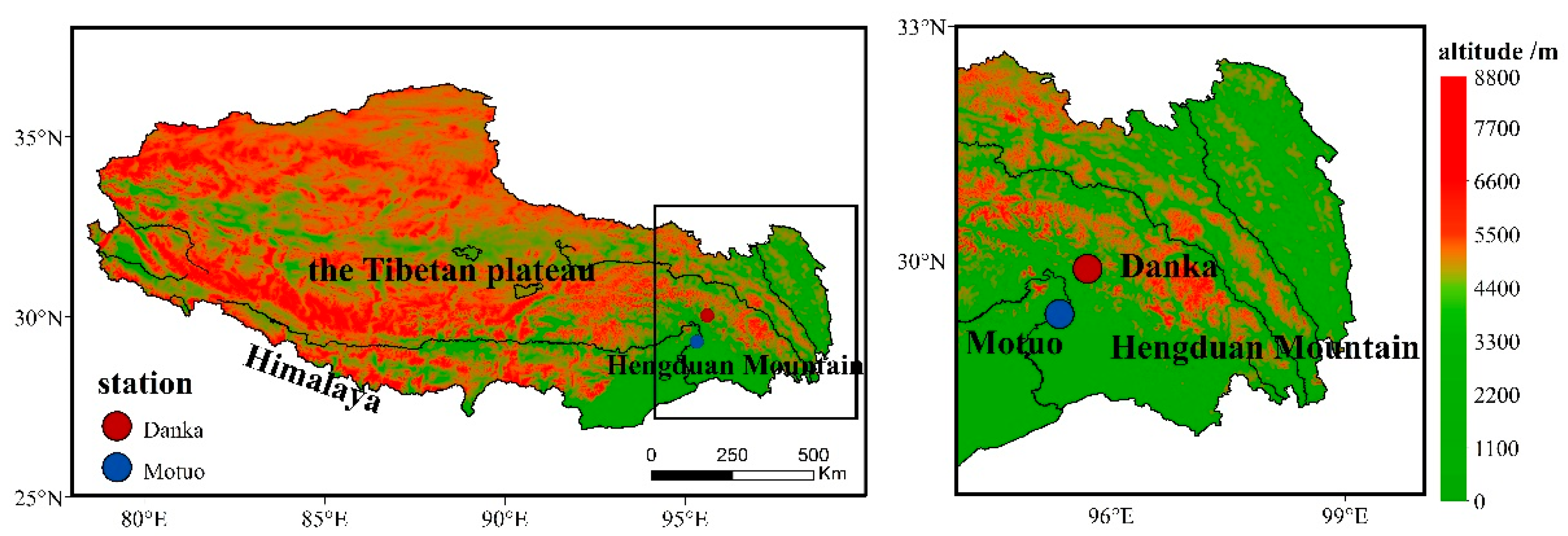
2.1. Study Area

The study area was the canyon area in the southeastern TP, and the research stations were Danka Station (29.89° N, 95.68° E, a.s.l. (above sea level) 2701 m) and Motuo Station (29.31° N, 95.32° E, a.s.l. 1154 m). Danka station is located in the northwestern part of Bomi County, Nyingchi City, Tibet Autonomous Region, on the southern bank of the Palongzangbo River Valley, and the underlying surface is mainly grassland. Motuo Station is located in the lower reaches of the Yarlung Zangbo River, Motuo County, and the underlying surface is mainly grassland. The topography of the observation area and the distribution of observation sites are shown in Figure 1.

2.2. Data

(1)

The global data assessment system (GDAS) data were obtained from the National Centers for Environmental Prediction (NCEP) of the United States (https://www.ready.noaa.gov/gdas1.php, accessed on 8 September 2020). The data were stored as 5 weeks for each month. The horizontal resolution of the data is 1° × 1°.

(2)

The NCEP/NCAR reanalysis data were obtained from the NCEP of the United States. We used the air temperature (air), u wind speed (uwnd), v wind speed (vwnd), and relative humidity (Rhum) data as the input for HYSPLIT_v4, and the horizontal resolution of the data is 2.5° × 2.5° (https://psl.noaa.gov/data/gridded/data.ncep.reanalysis.html, accessed on 10 May 2020).

(3)

The variables used in the reanalysis of the ERA-5 data (https://www.ecmwf.int/en/about/media-centre/science-blog/2017/era5-new-reanalysis-weather-and-climate-data, accessed on 18 October 2020) from the European Center for Medium Range Weather Forecasts (ECMWF) are the sensible heat flux (SSHF), the latent heat flux(SLHF), water vapor flux divergence integral (VIMDF, the vertical integral of the moisture flux is the horizontal rate of flow of moisture, per meter across the flow, for a column of air extending from the surface of the Earth to the top of the atmosphere), and the monthly mean water vapor flux from north to east. The horizontal resolution of the data is 0.1° × 0.1°. The time range of the data used in this study is from 1989 to 2019.

2.3. Water Vapor Transport Trajectory Model (HYSPLIT_v4)

The HYSPLIT_v4 model is a professional model for calculating and analyzing the transport and diffusion trajectories of air pollutants. It was jointly developed by the Air Resources Laboratory of the National Oceanic and Atmospheric Administration (NOAA) of the United States and the Australian Meteorological Service in the past 20 years [39,40]. The HYSPLIT_v4 model is a mixed Eulerian-Lagrangian model, in which the Lagrangian method is used for the advection and diffusion. The model is usually used to track the movement direction of the particles or gas carried by the airflow, and it can be used to forecast the wind situation in real time, to analyze precipitation, and to study the trajectory. In this study, the HYSPLIT_v4 model was used to simulate the water vapor transport from November 2018 to October 2019 at Danka and Motuo stations in the canyon area of southeastern Tibet, and the water vapor transport trajectory was studied. The model uses 11-day backward water vapor transport trajectory simulation, and the top height of the model is 10 km. The characteristics of the water vapor trajectories in different seasons were obtained.

2.4. Singular Value Decomposition (SVD) Method

The SVD method is based on the maximum covariance between two element fields. It is an effective diagnostic analysis method for studying the correlation structure of two fields. It is suitable for climate diagnostic analysis and for studying the teleconnections between large-scale meteorological fields. Compared with typical correlation analysis methods, the singular value decomposition method can maximally separate the independent coupling distribution patterns of the two meteorological fields. These distribution patterns reveal the spatial relationship and the temporal correlation between the two meteorological fields in order to determine the real teleconnection pattern and the key area of influence. From the spatial distribution pattern of the modal anisotropy correlation, we found the large value region of anisotropy correlation coefficient in the left and right fields, which represents the key region of the interactions between the left and right fields. The anisotropy correlation coefficients between the two meteorological element fields can be used to analyze their relationship. The Monte Carlo method was used to test the significance of the SVD results.

3. Results Analysis

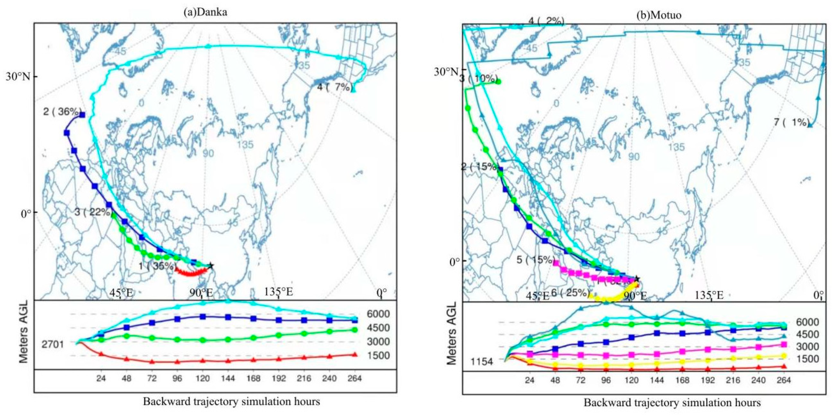
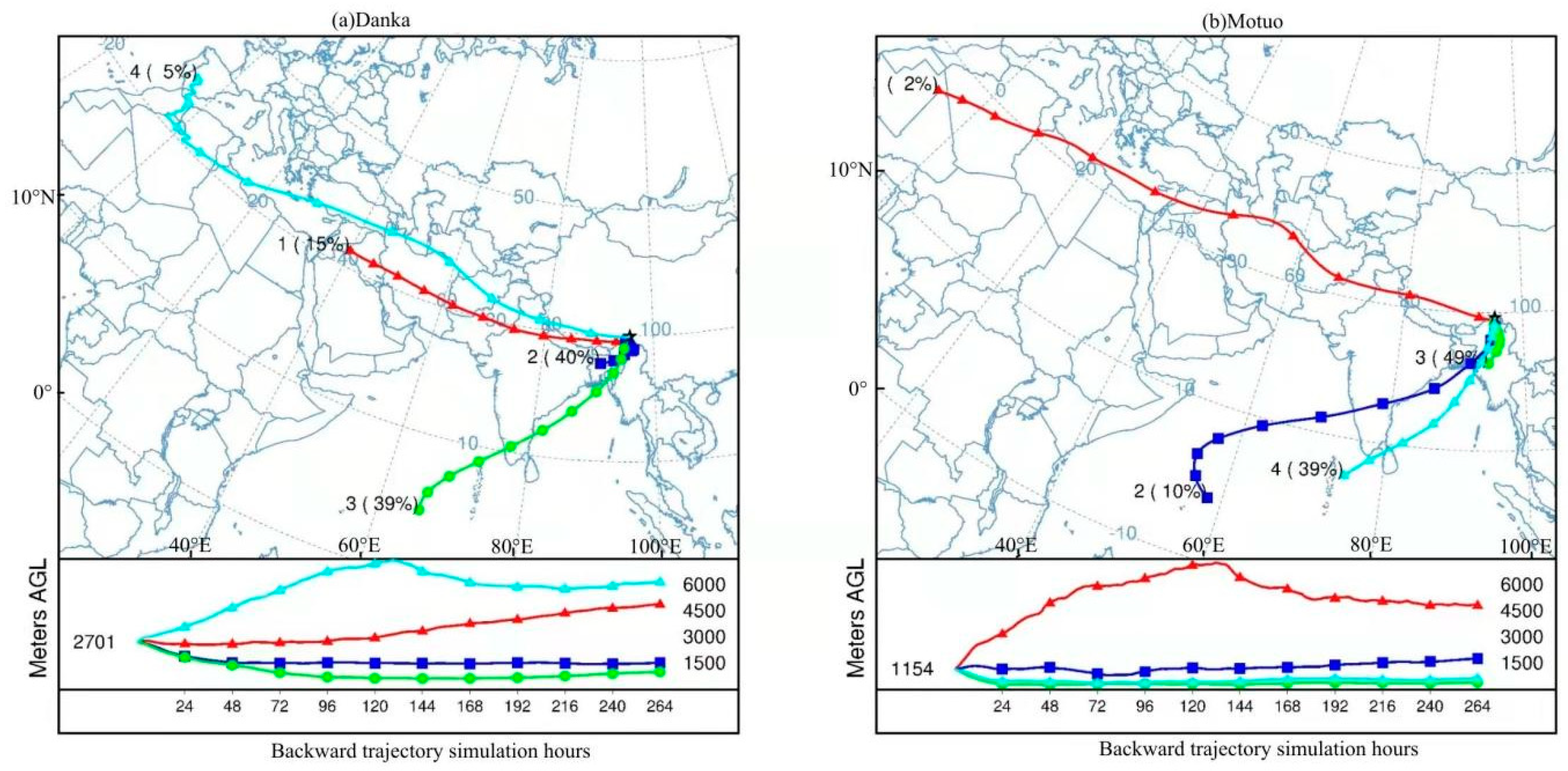
3.1. Water Vapor Transport Trajectories in the Canyon Area in Southeastern Tibet

Figure 2 shows the water vapor transport track at Danka Station and Motuo Station during the non-Asian monsoon season (non-AMS) (i.e., spring) for 11 days (the map projection is the Lambert projection). The northwest air flow is the main water vapor source at the two stations in the non-AMS. Seven percent of the water vapor at Danka Station came from the northeastern part of the Pacific Ocean, passed over Canada, passed over the Arctic Ocean, turned to the northwest over the Norwegian Sea, and reached Danka Station. Similarly, Motuo Station received a small amount of water vapor from the northern Pacific, 25% from India, 40% from the northwest path, and 32% from the nearby area to the west. Compared with the spring atmospheric circulation pattern on the TP, strong westerlies occurred to the south of the plateau during spring and were the main water vapor transport channels in the southeastern gorge area of Tibet. The high terrain of the plateau affected the wind flow around this latitude, forming a pattern characterized by a southern trough and a northern Ridge. The northwestward air flow of the northern ridge delivered about 40% of the water vapor to southeastern Tibet during the non-AMS. Based on the height of the water vapor transmission channels, the water vapor transmission channel in the southwest was below 3000 m, while the water vapor transmission channel in the west and the northwest water vapor transport height reached 4500 m.

Compared with the sources of water vapor transport during the non-AMS (spring), and the main water vapor source path of the two stations came from the southwest air flow (Figure 3). During the Asian monsoon season (AMS) (i.e., summer), 20% of the water vapor at Danka Station came from the northwest path and 80% came from the southwest, mainly from the Arabian Sea and the Bay of Bengal, whereas almost all of the water vapor at Motuo station came from the Arabian Sea. The height of the water vapor transmission path between the two stations through the Bay of Bengal was less than 1500 m. During this period, the South Asian Monsoon prevailed on the plateau, and the southwest winds at this time made a major contribution to the water vapor transport from the Bay of Bengal to this area, forming a main water vapor transport channel over southeastern Tibet and into inland China.

The water vapor transport in the canyon area of the southeastern TP is closely related to the Asian monsoon climate. Correlation analysis was conducted between the water vapor transport path and the circulation field, ground heating, and water vapor flux during the non-AMS and AMS in order to determine the mechanism by which the monsoon climate affects the water vapor transport path in the canyon area of the southeastern TP.

3.2. Effect of Surface Fluxes on Water Vapor Transport

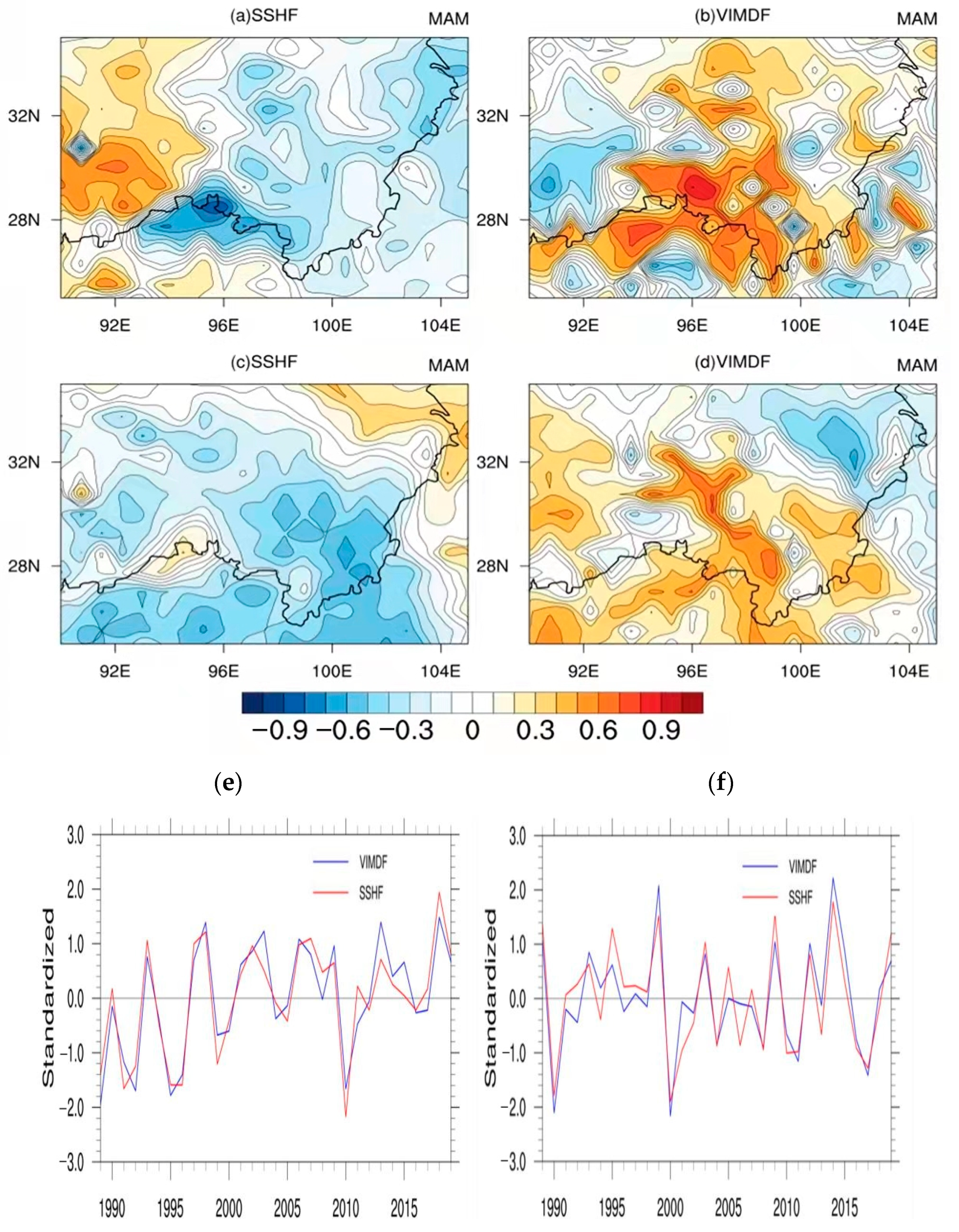
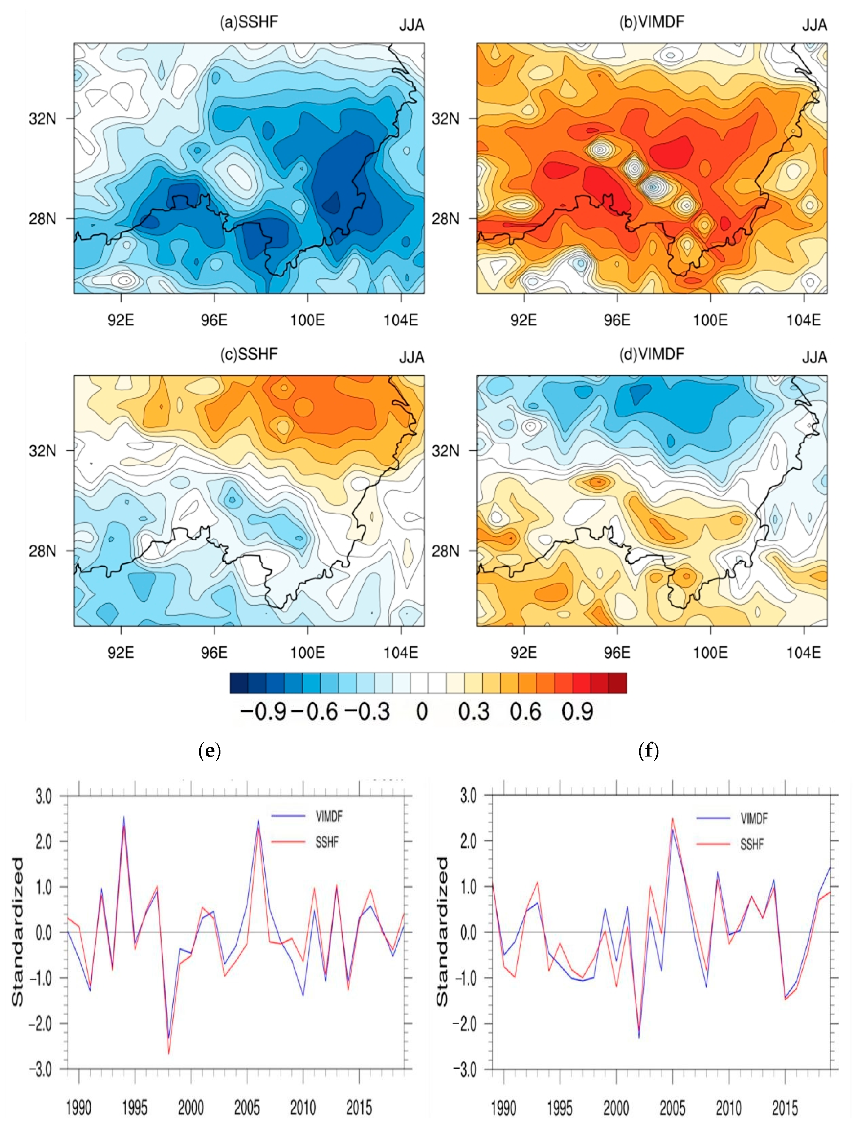
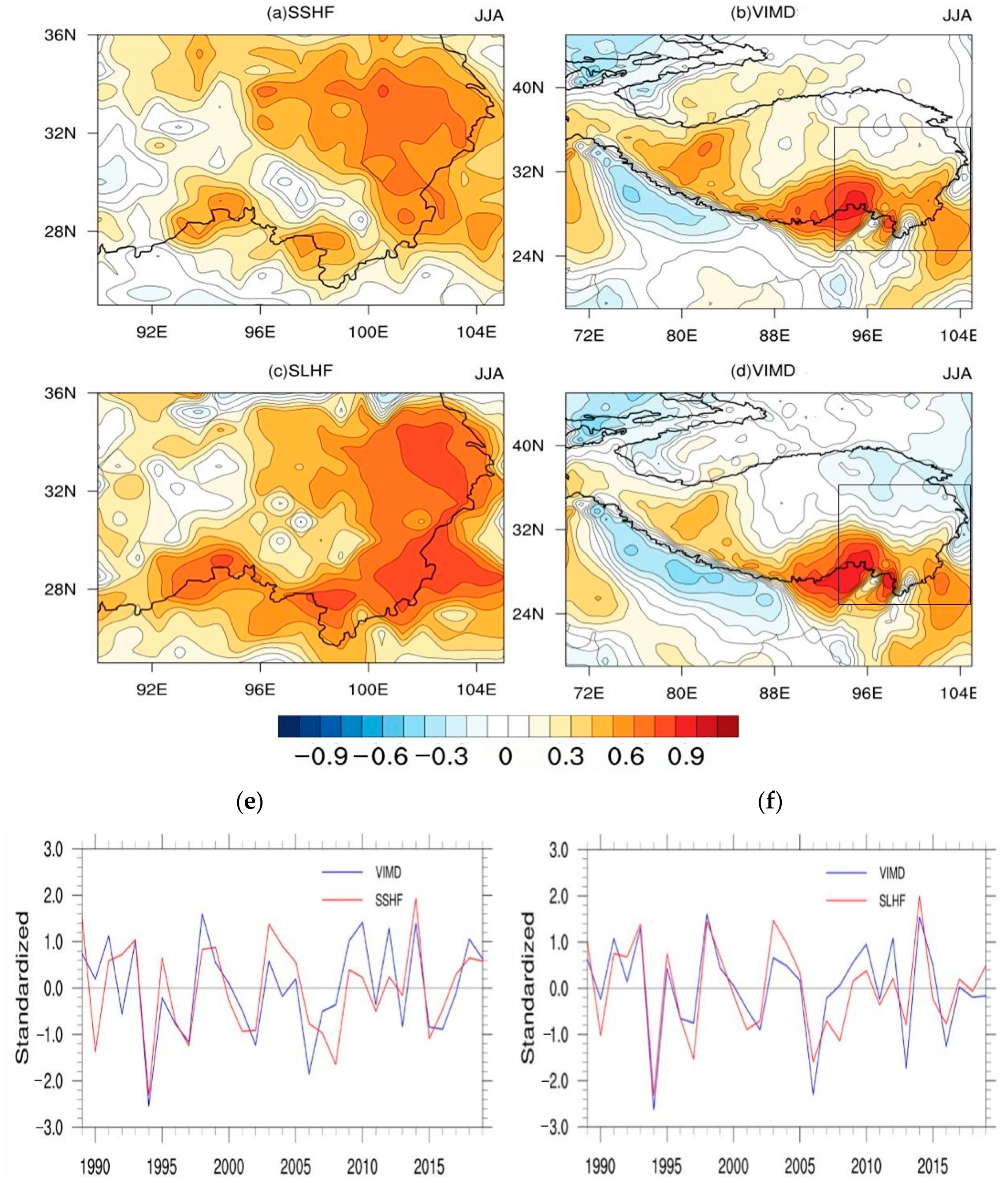
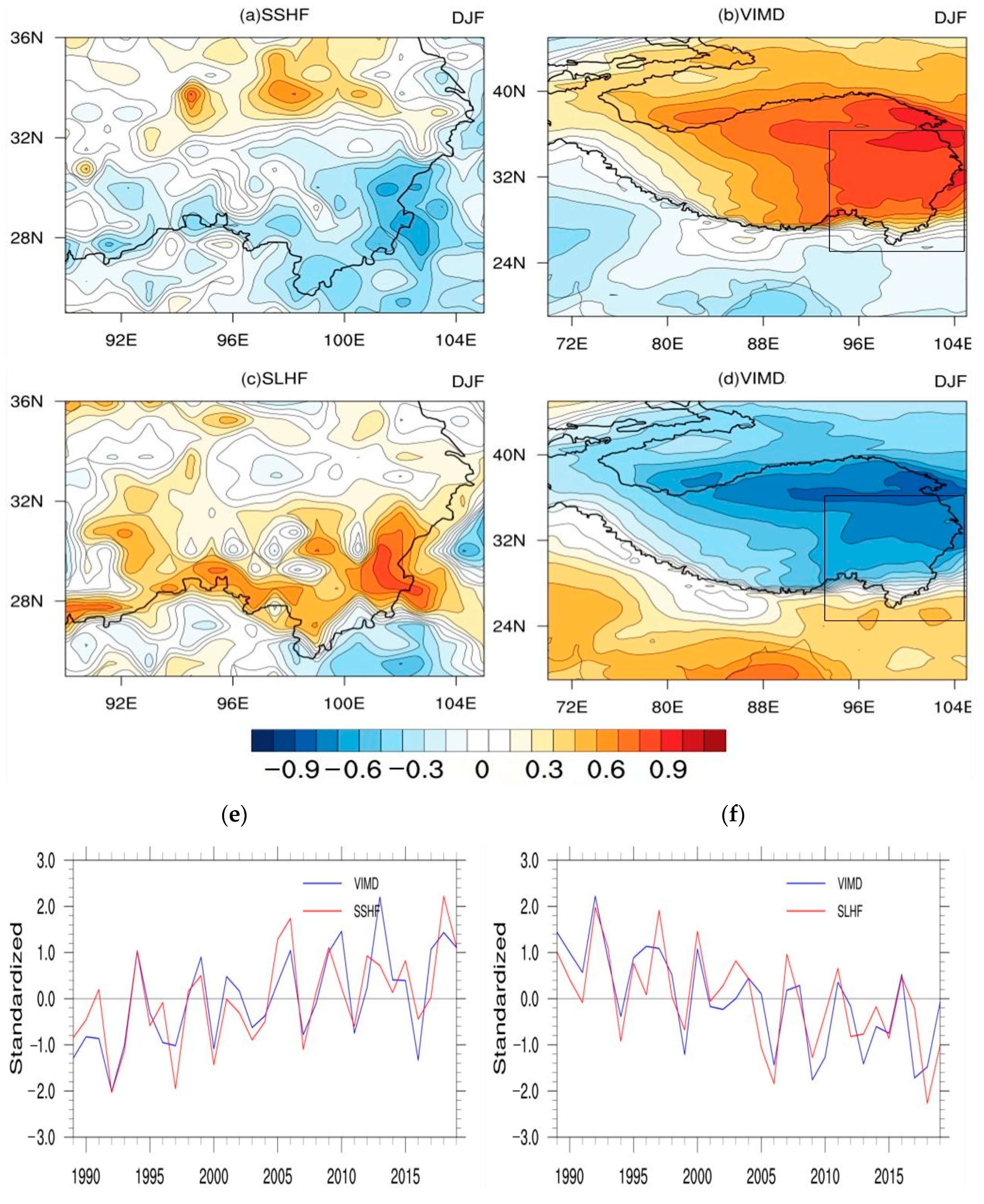
3.2.1. Relationship between Sensible Heat Flux and Water Vapor Flux Divergence in the Canyon Area of Southeastern Tibet

Based on the results of the water vapor transport simulation obtained using the HYSPLIT_v4 backward trajectory model (see Section 3.1), the water vapor transport in the canyon area of the southeastern TP exhibited significant climate characteristics during the AMS. In this section, we analyze the spatial relationship of the temporal correlation between the sensible heat and water vapor flux divergence from the perspective of the variations in the AMS. The water vapor flux divergence is a very important meteorological factor, which characterizes the water vapor transport. The SVD method was used to calculate the correlation coefficient (R) between the first four pairs of singular vector covariance contributions (SCFs), the cumulative covariance contributions (CSCFs), and the expansion coefficient. The time span was from 1989 to 2019 (

Table 1. SVD results of sensible heat field and water vapor flux divergence field.

Singular Vector	First Mode		Second Mode		Third Mode		Fourth Mode		CSCF (%)
	SCF (%)	R	SCF (%)	R	SCF (%)	R	SCF (%)	R
spring	33.25	0.93	16.74	0.91	13.19	0.83	8.39	0.86	80.17
summer	75.35	0.94	11.43	0.93	6.08	0.92	1.64	0.90	94.49
autumn	48.79	0.91	19.57	0.93	8.93	0.84	5.12	0.87	82.41
winter	38.03	0.89	20.66	0.85	12.22	0.82	7.15	0.87	78.06
all year	44.57	0.85	20.58	0.86	10.19	0.80	5.80	0.84	81.13

).

As can be seen from Table 1, the cumulative covariance contributions of the first four pairs of the coupling modes of the sensible heat and the water vapor flux divergence in each season and the whole year were greater than 78%, the covariance contribution rate of the first two modes was greater than 58%, and it reached 94.49% during the AMS, indicating that the first two pairs of coupling modes represent most of the characteristics of the sensible heat field and the water vapor flux divergence. In addition, the first two modes passed the 95% Monte Carlo test, so in this section, the first two coupling modes of the sensible heat field and the water vapor flux divergence field in southeastern Tibet are analyzed.

Figure 4 shows the results of the SVD anisotropy correlation analysis between the standardized anomaly of the sensible heat field and the standardized anomaly of the water vapor flux divergence field during the non-AMS. The first mode (Figure 4a,b) shows that the sensible heat in the southwestern and southwestern parts of southeastern Tibet was mainly positive. There was a significant negative value on the southern boundary line, and the values in the central and eastern regions were negative. In the corresponding water vapor flux divergence field, there was a positive center of the water vapor flux divergence on the southern boundary of the plateau and a negative region in the west. Except for the sporadic negative anomaly regions in the eastern, southern, and central parts of southeastern Tibet, the other regions were positive. Figure 4e,f show that the correlation coefficient between the sensible heat and water vapor flux divergence of the first mode is 0.93. There is a significant positive correlation between the sensible heat flux field and the water vapor flux divergence field. This indicates that during the non-AMS, when the sensible heat of the western and southwestern parts of the southeastern Tibet increased (decreased) and the sensible heat of the eastern and central parts of the southeastern Tibet decreased (increased), the water vapor flux divergence in the eastern part of Tibet decreased (increased), while it increased (decreased) in the central and eastern regions. From the second type of modal space, we can see that the sensible heat field was significantly negative in the Hengduan Mountains on the southeastern part of the TP, and there was a positive area in the northeast. The negative anomaly area in the northeastern part of southeastern Tibet corresponded to the water vapor flux divergence, and the rest of the areas were in the same positive region. The two large value areas corresponded to each other. The correlation coefficient between the sensible heat field and the whole water vapor flux divergence field of the second mode reached 0.91, indicating that when the sensible heat of the northeast area increased (decreased) during the non-AMS, the sensible heat in the rest of the areas decreased (increased), the water vapor flux divergence in the northeastern region decreased (increased), and it increased (decreased) in the rest of the areas.

The AMS is the main season for water vapor transport. The results of the SVD analysis of the sensible heat and the water vapor flux divergence fields during the AMS show that the cumulative variance contribution of the first four modes of the two fields reached 94.49%, which represents most of the characteristics of the sensible heat and the moisture flux divergence fields during the AMS (Table 1). The first mode of the SVD analysis of the summer surface flux field and the moisture flux divergence field shows that the sensible heat field was a negative region with a uniform type, and there was a significant negative value region on the southern and eastern boundaries of the plateau (Figure 5a–d). The whole water vapor flux divergence field was clearly positive in southeastern Tibet. The correlation coefficient between the sensible heat and the moisture flux divergence of the first mode was 0.94 during the AMS, indicating that there was a clear positive correlation between the sensible heat and the water vapor flux divergence fields. That is, when the sensible heat decreased (increased) during the AMS, the water vapor flux divergence increased (decreased), and the large negative area on the southern boundary and the southeast boundary was the key area and affected the whole water vapor flux divergence during the AMS. The contribution of the second mode’s covariance was 11.43%, and the significant positive area of the sensible heat field was located in the northern part of southeastern Tibet. The negative value area was located in the southwest, while the right field was opposite to this distribution. The correlation coefficient for the sensible heat and water vapor flux divergence fields was 0.93, exhibiting a positive correlation, indicating that the sensible heat field in the canyon area of southeastern Tibet increased in the northeast during the AMS. In addition, when it decreased in the southwest, the water vapor flux divergence field decreased in the northeast and increased in the southwest. The time series changes in the sensible heat and the water vapor flux divergence fields of the first two modes were basically synchronous (Figure 5e,f), and the fluctuation amplitude was large.

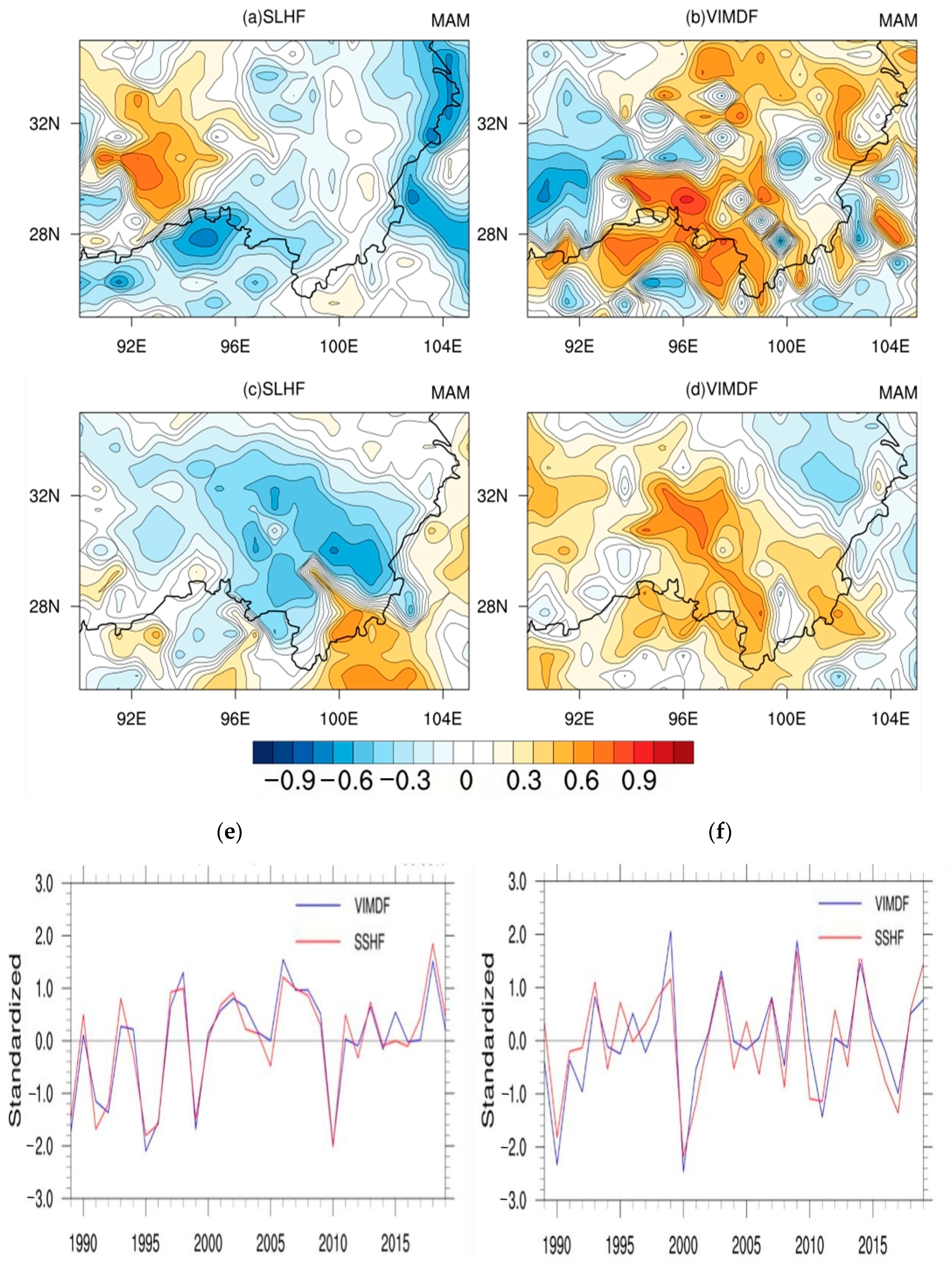
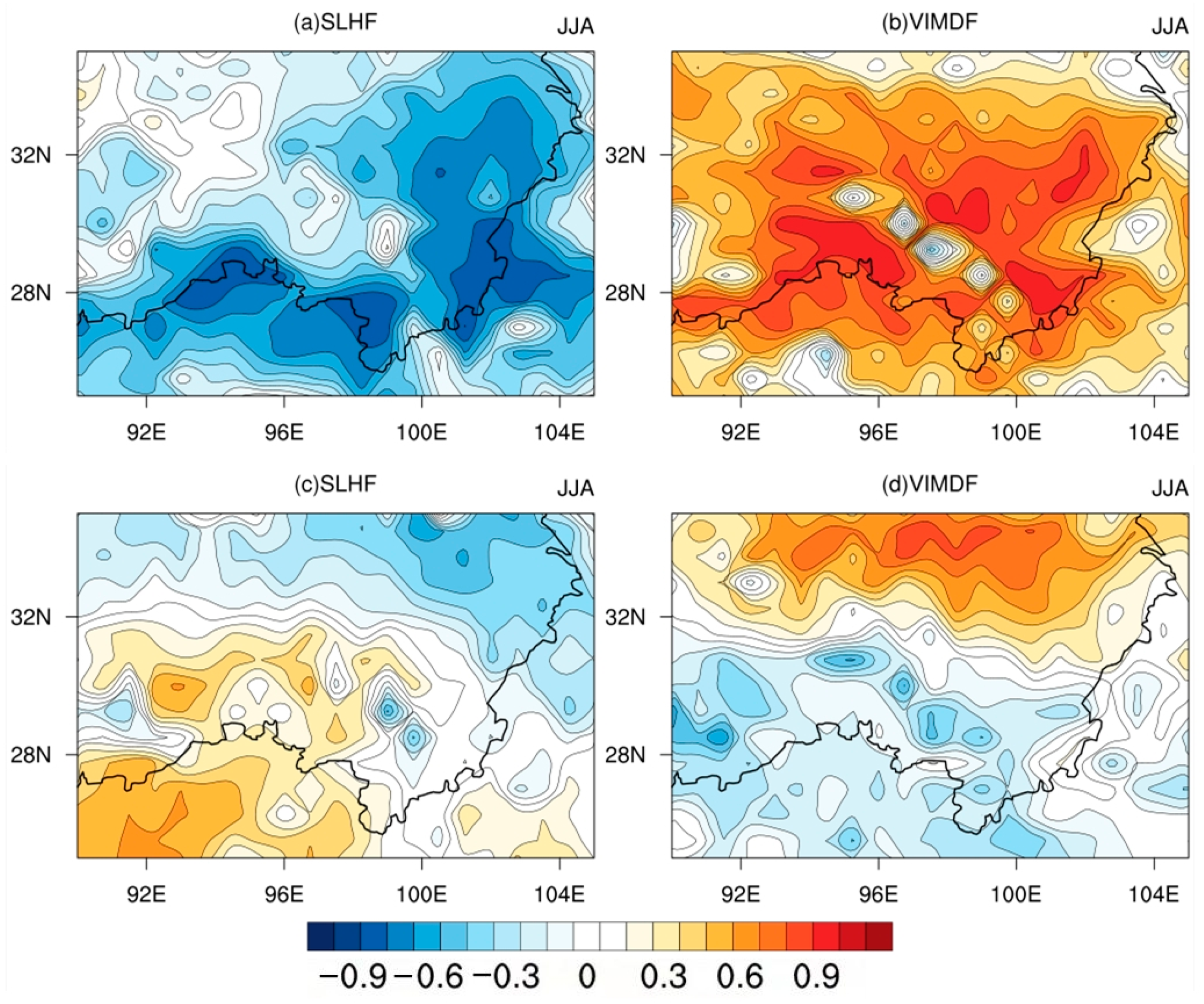
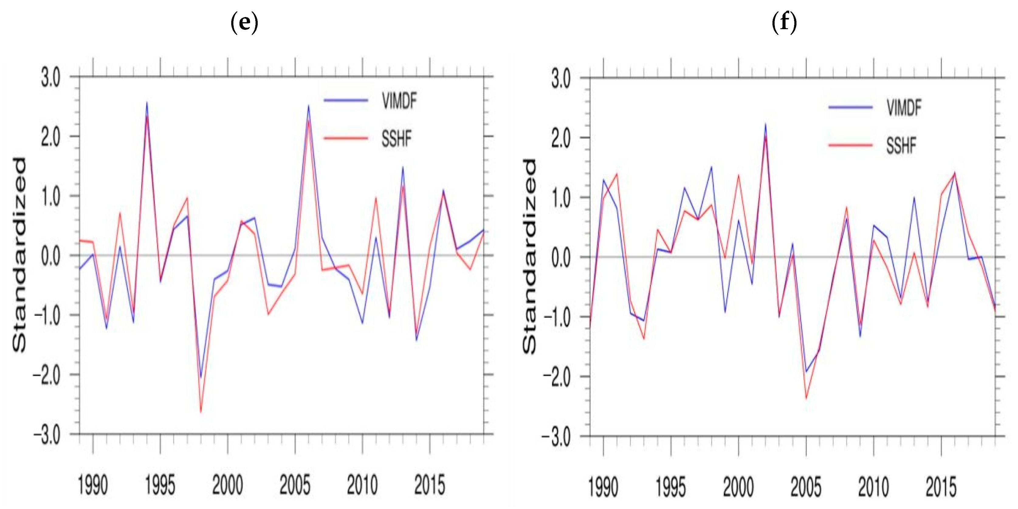
3.2.2. Relationship between the Latent Heat and the Water Vapor Flux Divergence in the Canyon Area of Southeastern Tibet

In this section, the SVD method is used to investigate the spatial relationship between the latent heat field and the water vapor flux divergence field. The latent heat field is the left field, and the water vapor flux divergence field is the right field. The covariance contribution (SCF), cumulative covariance contribution (CSCF), and correlation coefficient (R) of the first four pairs of singular vectors in each season were calculated (

Table 2. SVD results of latent heat field and water vapor flux divergence field.

Singular Vector	First Mode		Second Mode		Third Mode		Fourth Mode		CSCF (%)
	SCF (%)	R	SCF (%)	R	SCF (%)	R	SCF (%)	R
spring	36.98	0.95	20.20	0.86	12.87	0.82	8.85	0.83	78.10
summer	77.46	0.94	9.88	0.93	4.05	0.87	2.25	0.85	93.64
autumn	52.31	0.90	21.15	0.95	8.88	0.91	4.34	0.92	86.68
winter	43.20	0.93	17.11	0.89	12.91	0.93	5.94	0.89	79.15
all year	47.67	0.87	21.13	0.89	8.98	0.82	5.93	0.85	83.71

).

The cumulative covariance contributions of the first four pairs of coupling modes of the latent heat flux and the water vapor flux divergence in each season and the whole year were greater than 78%. The covariance contributions of the first two modes were greater than 57% and 93.64% during the AMS, respectively. It indicated that the first two pairs of coupling modes represent most of the characteristics of the latent heat flux and the water vapor flux divergence field (Table 2). The first two modes passed the 95% Monte Carlo test, so in this section, the first two coupling modes of the latent heat and water vapor flux divergence field in southeastern Tibet are analyzed.

Figure 6a–d shows the results of the SVD analysis of the normalized anomalies of the latent heat field and the water vapor flux divergence field during the non-AMS. From spatial distribution of the first mode, we can see that there was a positive region in the latent heat field, except for in the western region. The remaining areas were negative. There were remarkably positive values in the eastern and southern parts of the plateau. There was a negative value in the western part of the whole water vapor flux divergence field, and there were sporadic negative anomaly centers in the other areas. The correlation coefficient between the latent heat field and the water vapor flux divergence field of the first mode was 0.95, indicating that the two fields had a good positive correlation. That is, when the latent heat in southeastern Tibet decreased (increased) in the southwestern and eastern areas and the latent heat increased (decreased) in the west, the water vapor flux divergence increased (decreased) in the southwest and east and decreased (increased) in the west. In the second modal spatial distribution, the latent heat field was negative in the northwest and positive in the southeast, and the negative value of the whole water vapor flux divergence field was positive in the northeast. That is, when the sensible heat in southeastern Tibet was weak (strong) in northwest-southeast direction, the water vapor flux divergence field was strong (weak) in southwest-northeast direction. Based on the time series curve of the first mode and the second mode of the two fields, the correlations were 0.95 and 0.86, respectively (Figure 6e,f). The fluctuation trend was basically consistent, and the first mode time series exhibited an upward trend.

Figure 7a–d show the first mode of the spatial distribution of the latent heat field and the water vapor flux divergence field in southeastern Tibet during the AMS. It can be concluded that the latent heat field and the water vapor flux divergence field exhibited good consistent distributions, and the latent heat field during the AMS was negative. The significant negative centers were located on the plateau and the eastern and southern boundaries. The whole water vapor flux divergence field was a positive region. The positive centers were located in the southern and central parts of southeastern Tibet. The correlation coefficient for the first mode of the latent heat field and the water vapor flux divergence field was 0.94 during the AMS. There was a significant positive correlation. This shows that the water vapor flux divergence increased (decreased) when latent heat decreased in southeastern Tibet during the AMS. The second modal spatial distribution pattern was drawn as follows. When the latent heat field in southwestern Tibet increased in the southwest and decreased in the northeast, the water vapor flux divergence field in the total-column was reversed. Based on the corresponding time series of the first mode and the second mode, the change trend was more consistent, and the correlation coefficients reached 0.94 and 0.93, respectively, exhibiting the same phase of change (Figure 7e,f).

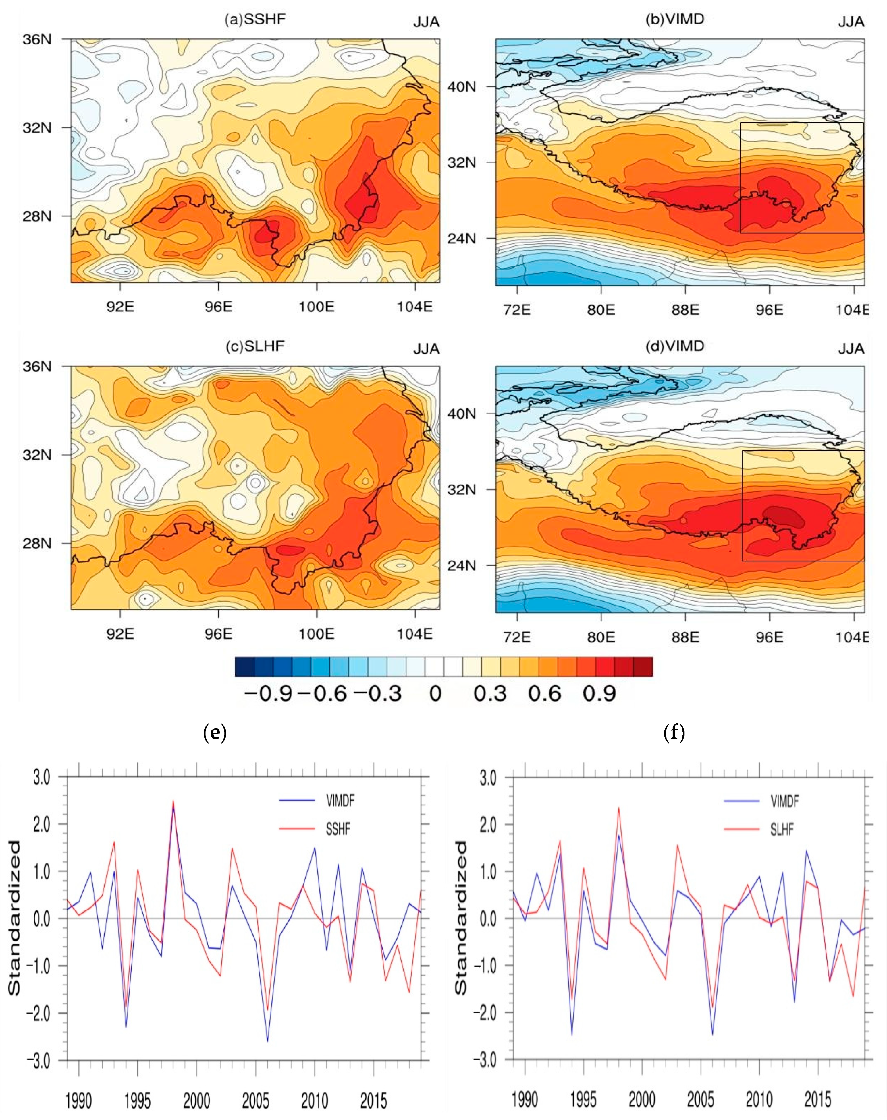
3.2.3. Relationships between the Surface Sensible Heat, Latent Heat, and Northward Water Vapor Flux

According to the trajectory simulation results of the HYSPLIT_v4 11-day backward trajectory, the source of the water vapor transport was closely related to the changes in the atmospheric circulation situation. The source of the water vapor transport was quite different during the non-AMS and the AMS. During the non-AMS, the water vapor in southeastern Tibet mainly came from a westward path, while during the AMS, the water vapor mainly came from a southwestward path, accounting for a relatively small number of westward paths. Therefore, the surface fluxes and the water vapor flux to the north and east in winter and summer are discussed in this section. Similarly, the surface sensible heat flux and the latent heat flux were taken as the left field in the SVD, the water vapor flux to the north and the water vapor flux to the east were taken as the right field, and the time period was from 1989 to 2019. The covariance contribution (SCF), cumulative covariance contribution (CSCF), and correlation coefficient (R) between the expansion coefficients of the first four pairs of singular vectors are shown in

Table 3. SVD Analysis of surface flux and northward water vapor flux in Southeast Tibet.

Singular Vector	SSHF				SLHF
	Summer		Winter		Summer		Winter
	SCF (%)	R	SCF (%)	R	SCF (%)	R	SCF (%)	R
1	68.15	0.83	76.41	0.78	61.89	0.85	78.52	0.80
2	20.82	0.74	13.31	0.78	24.91	0.77	11.70	0.81
3	5.86	0.76	4.66	0.82	6.40	0.79	3.96	0.83
4	2.08	0.84	1.94	0.87	3.03	0.81	1.81	0.82
CSCF (%)	96.90	/	96.32	/	96.23	/	95.98	/

. The north (east) water vapor flux refers to the horizontal water vapor velocity of a column of air extending from the Earth’s surface to the top of the atmosphere. A positive value represents the flux from the west (south) to the east (north). The mean cumulative variance contribution of the first mode to the SVD analysis of the surface flux and the northward and eastward vapor fluxes exceeded 61%. This represents the main characteristics of the relationship between the two physical quantity fields. The first mode passed the 95% level, so the first mode was analyzed in this section. The first four pairs of modal results are shown in Table 3.

For the first mode of the SVD analysis of the sensible heat and moisture during the non-AMS (Figure 8a,b), the results show that the sensible heat field was negative in both the southeast boundary and the southern part of the plateau, and the northern region was a positive anomaly, which was the key area affecting the northward water vapor flux during the same period. The northward water vapor flux field was positive, except for in the western region of the plateau, and the center of the positive anomaly was located in the central region. The correlation coefficient of the first mode was 0.78, indicating that there was a positive correlation between the sensible heat and the northward vapor flux. When the sensible heat increased in northeastern Tibet and decreased in southeastern Tibet and the southern part of the plateau, the water vapor flux in most parts of the plateau increased to the north and decreased to the west, and vice versa. From the corresponding time series (Figure 8e), it can be seen that the overall change trends of the surface flux and the northward water vapor flux were roughly the same. The fitting degree before 2008 was worse than that after 2008, and there were large fluctuations in 2009 and 2013.

There was also a significant coupling mode between the latent heat and northward water vapor flux during the non-AMS (Figure 8c,d). In the first mode, the contribution of the variance was 78.52%, and the correlation coefficient of the latent heat and the northward water vapor flux fields reached 0.8. The distribution characteristics of the time series were similar to those of the sensible heat field. The first mode was similar to the first mode of the sensible heat and the plateau’s northward moisture flux. The difference is that in the sensible heat field, the values were negative in northern and northwestern Tibet, while the northward water vapor flux field moved eastward. However, the whole plateau was still a positive anomaly, and the western part was negative. The correlation coefficient of the first mode was 0.8. This shows that when the surface latent heat increased in the western, central, southern, and eastern parts of the plateau in winter, the northward water vapor flux increased in most parts of the plateau and decreased in the western part, and vice versa (Figure 8f).

During the AMS, the relationship between the surface flux field and the northward water vapor flux field was more pronounced. There were significant coupling modes between the sensible and latent heat fluxes and the northward water vapor transport flux during the AMS, and the correlation coefficients were 0.83 and 0.85, respectively (Figure 9e,f). The sensible and latent heat flux fields had consistent positive values (Figure 9a,c). The large values were located in the eastern part of southeastern Tibet and the southern boundary of the plateau, which were the key areas in which the summer climate influenced the northward water vapor flux. The northward water vapor flux field was basically positive on the main part of the plateau, and the area with the largest positive value was in the southern part of southeastern Tibet. There was a good positive correlation between the surface sensible and latent heat fluxes and the northward water vapor flux, that is, when the sensible and latent heat fluxes increased (decreased) in the eastern part of southeast Tibet and the southern boundary of the plateau during the AMS, the northward water vapor flux in the main part of the plateau increased, especially in southeastern Tibet, and decreased in the Himalayas in southern Tibet. It can be seen from the time series diagram that the change trend of the surface flux field in southeastern Tibet was consistent with that of the northward water vapor flux field during the AMS (Figure 9e,f).

3.2.4. Influences of the Surface Sensible Heat and Latent Heat on the Water Eastward Vapor Flux

Table 4. SVD Analysis of surface flux and eastward water vapor flux in Southeast Tibet.

Singular Vector	SSHF				SLHF
	Summer		Winter		Summer		Winter
	SCF (%)	R	SCF (%)	R	SCF (%)	R	SCF (%)	R
1	83.37	0.77	73.02	0.80	87.85	0.85	72.01	0.79
2	11.22	0.63	19.55	0.71	7.88	0.74	19.51	0.71
3	2.29	0.79	2.83	0.74	2.12	0.71	3.64	0.89
4	1.68	0.80	2.08	0.79	0.87	0.80	2.31	0.84
CSCF (%)	98.55	/	97.48	/	98.72	/	97.46	/

shows the contribution rates and correlation coefficients of the first four pairs of principal component modes of the variance for the SVD analysis of the surface fluxes and eastward water vapor flux in southeast Tibet. It can be seen that the contribution rate of the cumulative variance of the first four pairs was greater than 97%, and there was a significant coupling mode. The analysis period was from 1989 to 2019. Similarly, the first mode of the SVD analysis passed the 95% level Monte Carlo test, so the first mode was mainly analyzed.

It can be seen from the time series diagram of the surface fluxes and the eastward water vapor flux during the non-AMS that the trends of the two-time series were quite consistent (Figure 10). The sensible heat and eastward water vapor flux exhibited fluctuating upward trends during the non-AMS, while the latent heat and eastward water vapor flux exhibited fluctuating downward trends. Figure 10e,f show the first mode of the corresponding time series of the SVD anisotropy between the surface fluxes and the eastward vapor flux during the non-AMS. Figure 10a,b show that the surface sensible heat field was negative in the northwest and positive in the southeast. The negative region was located at the boundary of the southeast plateau, and the eastward water vapor flux field was consistent as a whole. The main body of the plateau and the northern part of the plateau were positive. The high value area was located in the eastern part of Qinghai Province on northern part of the TP, and the southern part of the Himalayas was a consistent negative value area. The correlation coefficient between the sensible heat and the first mode of the eastward water vapor flux was 0.80, indicating that there was a positive correlation between the surface fluxes and the eastward water vapor flux fields. That is, when the sensible heat increased in the southeast and decreased in the northwest in the winter, the eastward water vapor flux increased over the plateau and decreased in the Himalayas, and vice versa.

It can be seen from Figure 10c,d that the latent heat had a good consistency. The positive high value area was located on the southeastern boundary of the plateau, and there was a small negative value area in the southeastern part. In the eastward water vapor flux field, the main body of the plateau and the area to the north were negative value areas, the high value area was in the Qinghai area on the northeastern part of the TP, and the positive area was in the southern part of the Himalayas, with a distribution opposite that of sensible heat field. The correlation coefficient of the first mode of the latent heat flux and the eastward vapor flux fields reached 0.79, which indicates that when the southeast latent heat accumulation increased in the southeast, the overall water vapor flux to the east decreased and that in the Himalaya Mountains increased, and vice versa.

The spatial distribution of the first mode of the SVD analysis of the sensible heat and latent heat fluxes during the AMS was consistent. In the first mode, the sensible and latent heat fields in southeast Tibet were positive, and the two large positive areas were located in southeastern Tibet (Figure 11a,c). This shows that this area was the key area in which the surface flux affected the eastward water vapor flux during the AMS. The eastward water vapor flux field was positive in the main part of the plateau and the Himalayas, and there were negative areas in the northwest and southwest (Figure 11b,d). The maximum positive area was located in southeastern Tibet, which corresponded well with the maximum positive area of the surface fluxes. There were significant coupling modes between the eastward water vapor flux and the sensible heat flux and latent heat flux during the AMS, and the correlation coefficients were 0.77 and 0.85, respectively. That is, when the sensible heat and latent heat fluxes increased in southeastern Tibet during the AMS, the water vapor flux from the main part of the plateau and the Himalayas to the east increased, and vice versa. It can be seen from the time series diagram that the change trend corresponded well and the fluctuation range was large (Figure 11e,f).

4. Summary and Conclusions

In this study, the 11-day backward trajectories of two observation stations located in the southeastern Tibetan Canyon from November 2018 to October 2019 were analyzed using the HYSPLIT_v4 backward trajectory model. Then the SVD method was used to analyze the relationships between the sensible heat and latent heat and the water vapor flux divergence in the southeastern Tibet gorge region. Due to the effects of the atmospheric circulation patterns and seasonal heat fluxes, the patterns of the moisture sources for southeastern Tibet exhibited significant seasonal differences. The main conclusions of this study are as follows.

(1)

The sources of the water vapor were different during the Asian monsoon and non-Asian monsoon seasons, and the main sources of the water vapor in the study area during the non-AMS were from the west and southwest. During the AMS, there was mainly southwest air flow and a small amount of southeast air flow in the lower layer. The westerly flow and northwesterly flow were the main sources of water vapor in winter. During the AMS, the southwestern water vapor transport accounted for more than half of the total. There was a certain correlation between the transportation height of each station and the source of water vapor. The height of the water vapor transportation channel of the western air flow was higher than 3000 m, and the height of the water vapor transportation channel of the southwestern and southeastern air flows was about 2000 m.

(2)

The sensible heat and latent heat in the northern part of the southeastern Tibet Canyon during the non-AMS were directly proportional to the change in the northward water vapor flux in the central and eastern parts of the plateau. During the AMS, the sensible heat and latent heat were directly proportional to the northward water vapor flux. When the sensible heat and latent heat decreased during the non-AMS, the eastward water vapor flux increased. The sensible heat and latent heat were negatively correlated with the eastward water vapor flux, while the sensible heat and latent heat were positively correlated with the eastward water vapor flux during the AMS.

(3)

There was a negative correlation between the surface fluxes and the water vapor flux divergence in this area. The southwest boundary of southeast Tibet was the key area affecting the water vapor flux divergence. When the surface sensible and latent heat fluxes increased in southeastern Tibet, the divergence of the water vapor flux decreased, that is, the water vapor transport to the region was weakened. When the sensible and latent heat fluxes decreased, the divergence of water vapor flux increased and the water vapor transport increased.

(4)

During the non-AMS, when the sensible heat in the canyon area of southeastern Tibet decreased, the eastward water vapor flux increased. Additionally, the northward water vapor fluxes on the plateau east of 75° E increased, while they decreased on the western part. When the latent heat increased, the eastward water vapor flux decreased, and the sensible heat and latent heat were negatively correlated with the northward water vapor flux during the non-AMS. That is, when the surface flux increased in southeastern Tibet, the water vapor transport from west to east increased. During the AMS, when the sensible heat and latent heat in southeastern Tibet increased as a whole, the eastward water vapor flux in the total-column in southeastern Tibet increased. This indicates that when the surface flux in southeastern Tibet increased during the AMS, the water vapor transport increased from west to east.

Our results show that the source of water vapor in the study area is different in different seasons, which will provide a certain theoretical basis for further research on the extreme precipitation of the Tibetan Plateau in the future. It is of great value to further study the different source areas and density of water vapor sources to improve extreme precipitation forecasts. In addition, some questions remain to be addressed. For example, this article only analyzes the seasonal characteristics of water vapor sources in southeastern Tibet from 2018 to 2019, only the data of the past 30 years is selected for analysis. Why were there large fluctuations in 2009 and 2013, whether the VIMDF is mainly influenced by the surface thermal effect on the TP, and whether the relationship is regulated by other external forcing factors, such as sea surface temperature (SST). Cui et al. (2015) pointed out that during the positive phase of the North Atlantic Oscillation (NAO) in winter, it can inspire a stable downstream Rossby wave train, inducing the Asian subtropical westerly jet to intensify and the India-Burma trough to deepen, and it also increases the snow depth on the TP in winter, followed by a positive SSHF anomaly in spring in most areas of the TP [41]. What are the synergetic effect and contribution rates of the NAO and the SSHF on the TP? These issues need further study.

References

- Li, G.P. Dynamic Meteorology of Qinghai-Tibet Plateau; Meteorological Press: Beijing, China, 2002. [Google Scholar]
- Xu, X.; Lu, C.; Shi, X.; Gao, S. World water tower: An atmospheric perspective. Geophys. Res. Lett. 2008, 35. [Google Scholar] [CrossRef]
- Jane, Q. The third pole. Nature 2008, 454, 393–396. [Google Scholar]
- Yao, T.; Masson-Delmotte, V.; Gao, J.; Yu, W.; Yang, X.; Risi, C.; Sturm, C.; Werner, M.; Zhao, H.; He, Y.; et al. A review of climatic controls on δ18O in precipitation over the Tibetan Plateau: Observations and simulations. Rev. Geophys. 2013, 51, 525–548. [Google Scholar] [CrossRef]
- Wu, G.; Liu, Y.; Zhang, Q.; Duan, A.; Wang, T.; Wan, R.; Liu, X.; Li, W.; Wang, Z.; Liang, X. The Influence of Mechanical and Thermal Forcing by the Tibetan Plateau on Asian Climate. J. Hydrometeorol. 2007, 8, 770–789. [Google Scholar] [CrossRef] [Green Version]
- Meng, X.N.; Liu, H.Z.; Du, Q.; Liu, Y.; Xu, L.J. Factors controlling the latent and sensible heat fluxes over erhai lake under different atmospheric surface layer stability conditions. Atmos. Ocean. Sci. Lett. 2020, 13, 400–406. [Google Scholar] [CrossRef]
- Ren, Q.; Zhou, C.Y.; Xia, Y.; Cen, S.X.; Long, Y. Interannual relationship between spring sensible heat flux over the eastern Tibetan Plateau and temperature in eastern China. J. Glaciol. Geocryol. 2019, 41, 783–792. [Google Scholar]
- Wang, J.; Tong, J.L.; Xiao, Y.Q.; Wu, X.Y.; Zhang, W.Y. The interannual variation of summer sensible heat flux in typical arid and semi-arid regions of East Asia. Arid Meteorol. 2018, 36, 203–211. [Google Scholar]
- Odhiambo, G.O.; Savage, M.J. Sensible heat flux by surface layer scintillometry and eddy covariance over a mixed grassland community as affected by bowen ratio and most formulations for unstable conditions. J. Hydrometeorol. 2009, 10, 479–492. [Google Scholar] [CrossRef]
- Zou, H.; Zhou, L.B.; Ma, S.P.; Wang, P.; Li, W.; Jia, A.G.; Gao, J.J.; Deng, Y. Local wind system in the Rongbuk valley on the northern slope of Mt. Everest. Geophys. Res. Lett. 2008, 35, 344–349. [Google Scholar] [CrossRef]
- Ye, D.Z. Meteorology of Qinghai Tibet Plateau; Science Press: Beijing, China, 1979. [Google Scholar]
- Zhang, Q.; Wang, R.; Yue, P.; Zhao, Y.D. Discussion on some scientific problems in the field of land air interaction under complex conditions. Acta Meteorol. Sin. 2017, 75, 39–56. [Google Scholar]
- Xu, X.; Zhao, T.; Lu, C.; Guo, Y.; Chen, B.; Liu, R.; Li, Y.; Shi, X. An important mechanism sustaining the atmospheric “water tower” over the Tibetan Plateau. Atmos. Chem. Phys. 2014, 14, 11287–11295. [Google Scholar] [CrossRef] [Green Version]
- Tao, S.; Ding, Y. Observational evidence of the influence of the Qinghai-Xizang (Tibet) Plateau on the occurrence of heavy rain and severe convective storms in China. Bull. Am. Meterol. Soc. 1981, 62, 23–30. [Google Scholar] [CrossRef]
- Liang, H. Distribution and Variation of Atmospheric Water Vapor over the Tibetan Plateau and Its Surrounding Areas. Ph.D. Thesis, Chinese Academy of Meteorological Sciences, Beijing, China, 2005. [Google Scholar]
- Liang, H.; Liu, J.M.; Zhang, J.C.; Bi, Y.M.; Wang, K.C. Research on Retrieval of the Amount of Atmospheric Water Vapor over Qinghai-Xizang Plateau. Plateau Meteorol. 2006, 025, 1055–1063. [Google Scholar]
- Jiang, J.X.; Fan, M.Z. A preliminary study on the relationship between TBB field and water vapor distribution over the Tibetan Plateau in summer. Plateau Meteorol. 2002, 21, 20–24. [Google Scholar]
- Ding, Y.G.; Jiang, Z.H. Universality of SVD method in meteorological field diagnosis and analysis. Acta Meteorol. Sin. 1996, 54, 365–372. [Google Scholar]
- Qu, Y.L.; Zhang, C.D. The distribution and structure of water vapour flux field over East Asia in summer. Plateau Meteorol. 1985, 4, 121–128. [Google Scholar]
- Massacand, A.C.; Wernli, H.; Davies, H.C. Heavy precipitation on the Alpine southside: An upper-level precursor. Geophys. Res. Lett. 1998, 25, 1435–1438. [Google Scholar] [CrossRef]
- Bertò, A.; Buzzi, A.; Zardi, D. Back—tracking water vapour contributing to a precipitation event over Trentino: A case study. Meteorol. Z. 2004, 13, 189–200. [Google Scholar] [CrossRef]
- James, P.; Stohl, A.; Spichtinger, N.; Eckhardt, S.; Forster, C. Climatological aspects of the extreme European rainfall of August 2002 and a trajectory method for estimating the associated evaporative source regions. Nat. Hazards Earth Syst. Sci. 2004, 4, 733–746. [Google Scholar] [CrossRef] [Green Version]
- Sodemann, H.; Stohl, A. Asymmetries in the moisture origin of Antarctic precipitation. Geophys. Res. Lett. 2009, 36, 273–289. [Google Scholar] [CrossRef] [Green Version]
- Sodemann, H.; Schwierz, C.; Wernli, H. Interannual variability of Greenland winter precipitation sources: Lagrangian moisture diagnostic and North Atlantic Oscillation influence. J. Geophys. Res. 2008, 113, D03107. [Google Scholar] [CrossRef] [Green Version]
- Li, J.; Tao, T.; Pang, Z.; Tan, M.; Kong, Y.; Duan, W.; Zhang, Y. Identification of different moisture sources through isotopic monitoring during a storm event. J. Hydrometeorl. 2015, 16, 1918–1927. [Google Scholar] [CrossRef]
- Han, T.; Zhang, M.; Wang, S.; Qu, D.; Du, Q. Sub-hourly variability of stable isotopes in precipitation in the marginal zone of East Asian monsoon. Water 2020, 12, 2145. [Google Scholar] [CrossRef]
- Jiang, Z.; Ren, W.; Liu, Z.; Yang, H. Analysis of water vapor transportcharacteristics during the Vleiyu over the Yangtze-Huaihe River valley using the Lagrangian method. Acta Meteor Sin. 2013, 71, 295–304. [Google Scholar]
- Chu, Q.; Wang, Q.; Feng, G.; Jia, Z.; Liu, G. Roles of water vapor sources and transport in the intraseasonal and interannual variation in the peak monsoon rainfall over East China. Clim. Dyn. 2021, 57, 2153–2170. [Google Scholar] [CrossRef]
- Chen, Y.; Luo, Y. Analysis of Paths and Sources of Moisture for the South China Rainfall during the Presummer Rainy Season of 1979–2014. Acta Meteorol. Sin. 2018, 32, 744–757. [Google Scholar] [CrossRef]
- Sun, B.; Wang, H. Moisture Sources of Semiarid Grassland in China489 Using the Lagrangian Particle Model FLEXPART. J. Clim. 2014, 27, 2457–2474. [Google Scholar] [CrossRef]
- Tao, S.; Luo, S.; Zhang, H. The Qinghai-Xizang Plateau Meteorological Experiment (Qxpmex) May–August 1979. In Proceedings of the International Symposium on the Qinghai-Xizang Plateau and Mountain Meteorology, Beijing, China, 20–24 March 1986; pp. 3–13. [Google Scholar]
- Wang, J. Land surface process experiments and interaction study in China-From HEIFE to IMGRASS and GAME-TIBET/TIPEX. Plateau Meteorol. 1999, 18, 280–294. [Google Scholar]
- Ma, Y.; Yao, T.; Wang, J. Experimental study of energy and water cycle in Tibetan plateau—The progress introduction on the study of GAME/Tibet and CAMP/Tibet. Plateau Meteorol. 2006, 25, 344–351. [Google Scholar]
- Ma, Y.; Hu, Z.; Xie, Z.; Ma, W.; Wang, B.; Chen, X.; Li, M.; Zhong, L.; Sun, F.; Gu, L.; et al. A long-term (2005–2016) dataset of hourly integrated land-atmosphere interaction observations on the Tibetan Plateau. Earth Syst. Sci. Data (ESSD) 2020, 12, 2937–2957. [Google Scholar] [CrossRef]
- Dong, W.; Lin, Y.; Wright, J.S.; Ming, Y.; Xie, Y.; Wang, B.; Huang, W.; Huang, J.; Wang, L.; Tian, L.; et al. Summer rainfall over the southwestern Tibetan Plateau controlled by deep convection over the Indian subcontinent. Nat. Commun. 2016, 7, 10925. [Google Scholar] [CrossRef] [PubMed]
- Ma, Y.; Wang, Y.; Han, C. Regionalization of land surface heat fluxes over the heterogeneous landscape: From the Tibetan Plateau to the Third Pole region. Int. J. Remote. Sens. 2018, 39, 5872–5890. [Google Scholar] [CrossRef]
- Li, M.; Babel, W.; Tanaka, K.; Foken, T. Note on the application of planar-fit rotation for non-omnidirectional sonic anemometers. Atmos. Meas. Tech. 2013, 6, 221–229. [Google Scholar] [CrossRef] [Green Version]
- Zhong, L.; Ma, Y.; Hu, Z.; Fu, Y.; Hu, Y.; Wang, X.; Cheng, M.; Ge, N. Estimation of hourly land surface heat fluxes over the Tibetan Plateau by the combined use of geostationary and polar-orbiting satellites. Atmos. Chem. Phys. 2019, 19, 5529–5541. [Google Scholar] [CrossRef] [Green Version]
- Wernli, H. A Lagrangian-based analysis of extratropical cyclones II: A detailed case-study. Q. J. R. Meteorol. Soc. 1997, 123, 1677–1706. [Google Scholar] [CrossRef]
- Nieto, R.; Gimeno, L.; Trigo, R.M. A Lagrangian identificantion of major sources of Sahel moisture. Geophy. Res. Lett. 2006, 33, L18707. [Google Scholar] [CrossRef]
- Cui, Y.F.; Duan, A.M.; Liu, Y.M.; Wu, G.X. Interannual variability of the spring atmospheric heat source over the Tibetan Plateau forced by the North Atlantic SSTA. Clim. Dyn. 2015, 45, 1617–1634. [Google Scholar] [CrossRef]